
Date: 2019-12-25 22:33:47 CET, cola version: 1.3.2
Document is loading...
All available functions which can be applied to this res_list object:
res_list
#> A 'ConsensusPartitionList' object with 24 methods.
#>   On a matrix with 14581 rows and 58 columns.
#>   Top rows are extracted by 'SD, CV, MAD, ATC' methods.
#>   Subgroups are detected by 'hclust, kmeans, skmeans, pam, mclust, NMF' method.
#>   Number of partitions are tried for k = 2, 3, 4, 5, 6.
#>   Performed in total 30000 partitions by row resampling.
#>
#> Following methods can be applied to this 'ConsensusPartitionList' object:
#>  [1] "cola_report"           "collect_classes"       "collect_plots"         "collect_stats"
#>  [5] "colnames"              "functional_enrichment" "get_anno_col"          "get_anno"
#>  [9] "get_classes"           "get_matrix"            "get_membership"        "get_stats"
#> [13] "is_best_k"             "is_stable_k"           "ncol"                  "nrow"
#> [17] "rownames"              "show"                  "suggest_best_k"        "test_to_known_factors"
#> [21] "top_rows_heatmap"      "top_rows_overlap"
#>
#> You can get result for a single method by, e.g. object["SD", "hclust"] or object["SD:hclust"]
#> or a subset of methods by object[c("SD", "CV")], c("hclust", "kmeans")]
The call of run_all_consensus_partition_methods() was:
#> run_all_consensus_partition_methods(data = mat, mc.cores = 4)
Dimension of the input matrix:
mat = get_matrix(res_list)
dim(mat)
#> [1] 14581 58
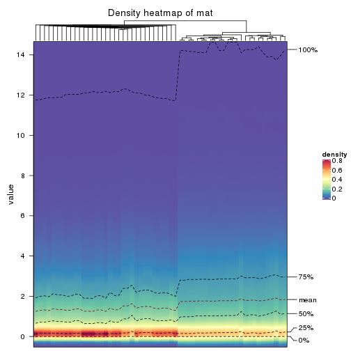
The density distribution for each sample is visualized as in one column in the following heatmap. The clustering is based on the distance which is the Kolmogorov-Smirnov statistic between two distributions.
library(ComplexHeatmap)
densityHeatmap(mat, ylab = "value", cluster_columns = TRUE, show_column_names = FALSE,
    mc.cores = 4)
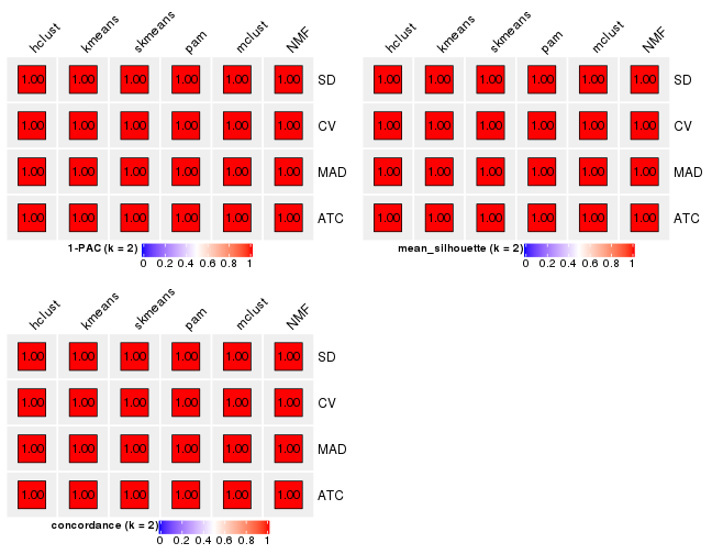
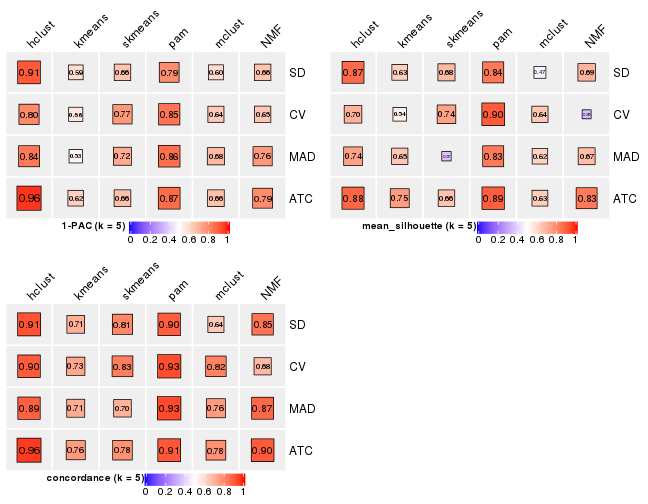
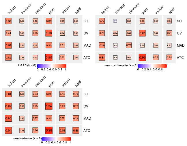
Folowing table shows the best k (number of partitions) for each combination
of top-value methods and partition methods. Clicking on the method name in
the table goes to the section for a single combination of methods.
The cola vignette explains the definition of the metrics used for determining the best number of partitions.
suggest_best_k(res_list)
| The best k | 1-PAC | Mean silhouette | Concordance | Optional k | ||
|---|---|---|---|---|---|---|
| SD:kmeans | 2 | 1.000 | 1.000 | 1.000 | ** | |
| SD:skmeans | 2 | 1.000 | 1.000 | 1.000 | ** | |
| SD:pam | 2 | 1.000 | 1.000 | 1.000 | ** | |
| SD:mclust | 2 | 1.000 | 1.000 | 1.000 | ** | |
| CV:kmeans | 2 | 1.000 | 1.000 | 1.000 | ** | |
| CV:skmeans | 2 | 1.000 | 1.000 | 1.000 | ** | |
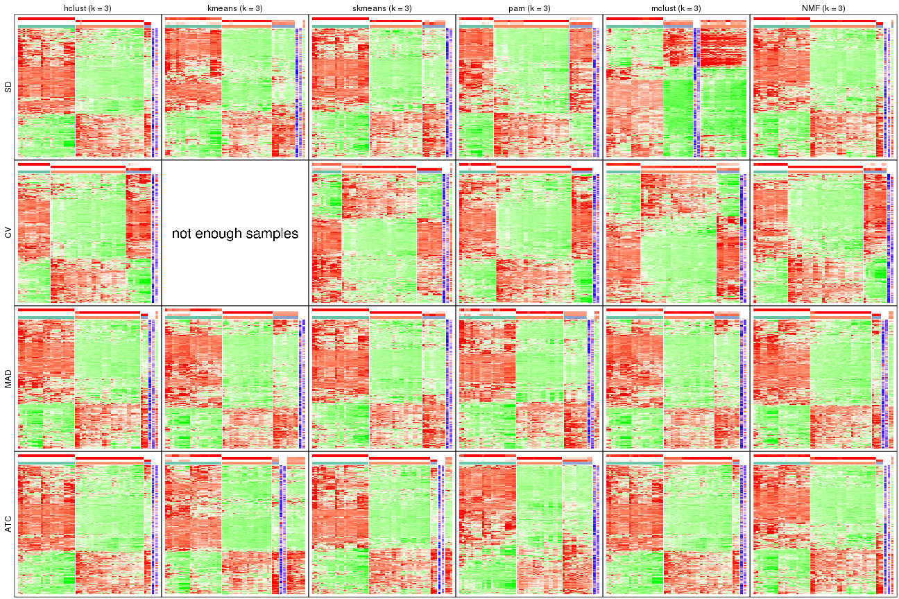
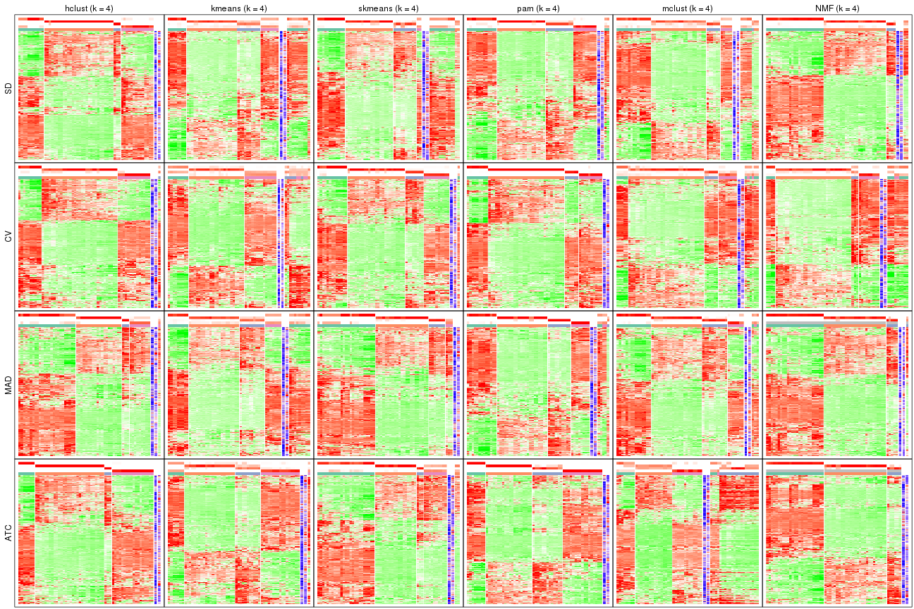
| CV:pam | 4 | 1.000 | 0.993 | 0.995 | ** | 2,3 |
| CV:mclust | 2 | 1.000 | 0.999 | 1.000 | ** | |
| MAD:hclust | 3 | 1.000 | 0.970 | 0.987 | ** | 2 |
| MAD:kmeans | 2 | 1.000 | 1.000 | 1.000 | ** | |
| MAD:pam | 2 | 1.000 | 1.000 | 1.000 | ** | |
| MAD:mclust | 2 | 1.000 | 1.000 | 1.000 | ** | |
| ATC:kmeans | 2 | 1.000 | 1.000 | 1.000 | ** | |
| ATC:skmeans | 3 | 1.000 | 0.948 | 0.979 | ** | 2 |
| ATC:mclust | 2 | 1.000 | 1.000 | 1.000 | ** | |
| SD:NMF | 3 | 0.987 | 0.964 | 0.982 | ** | 2 |
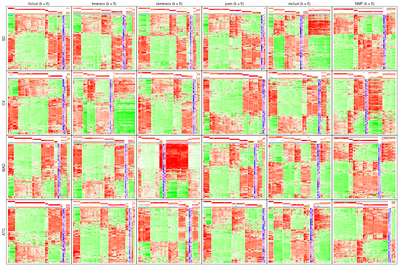
| ATC:hclust | 5 | 0.962 | 0.879 | 0.955 | ** | 2,3,4 |
| CV:NMF | 3 | 0.957 | 0.953 | 0.966 | ** | 2 |
| CV:hclust | 3 | 0.950 | 0.979 | 0.987 | * | 2 |
| ATC:pam | 6 | 0.945 | 0.959 | 0.976 | * | 2 |
| MAD:NMF | 4 | 0.927 | 0.919 | 0.951 | * | 2,3 |
| ATC:NMF | 4 | 0.922 | 0.916 | 0.957 | * | 2,3 |
| SD:hclust | 5 | 0.905 | 0.871 | 0.915 | * | 2,3 |
| MAD:skmeans | 3 | 0.902 | 0.980 | 0.981 | * | 2 |
**: 1-PAC > 0.95, *: 1-PAC > 0.9
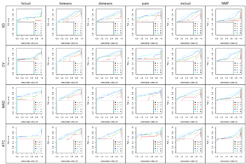
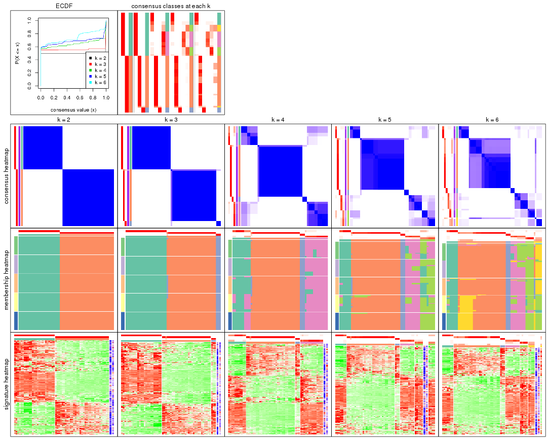
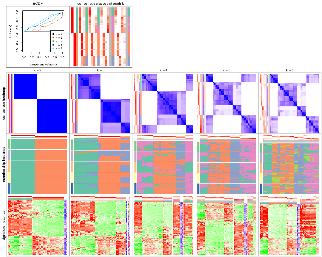
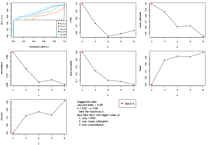
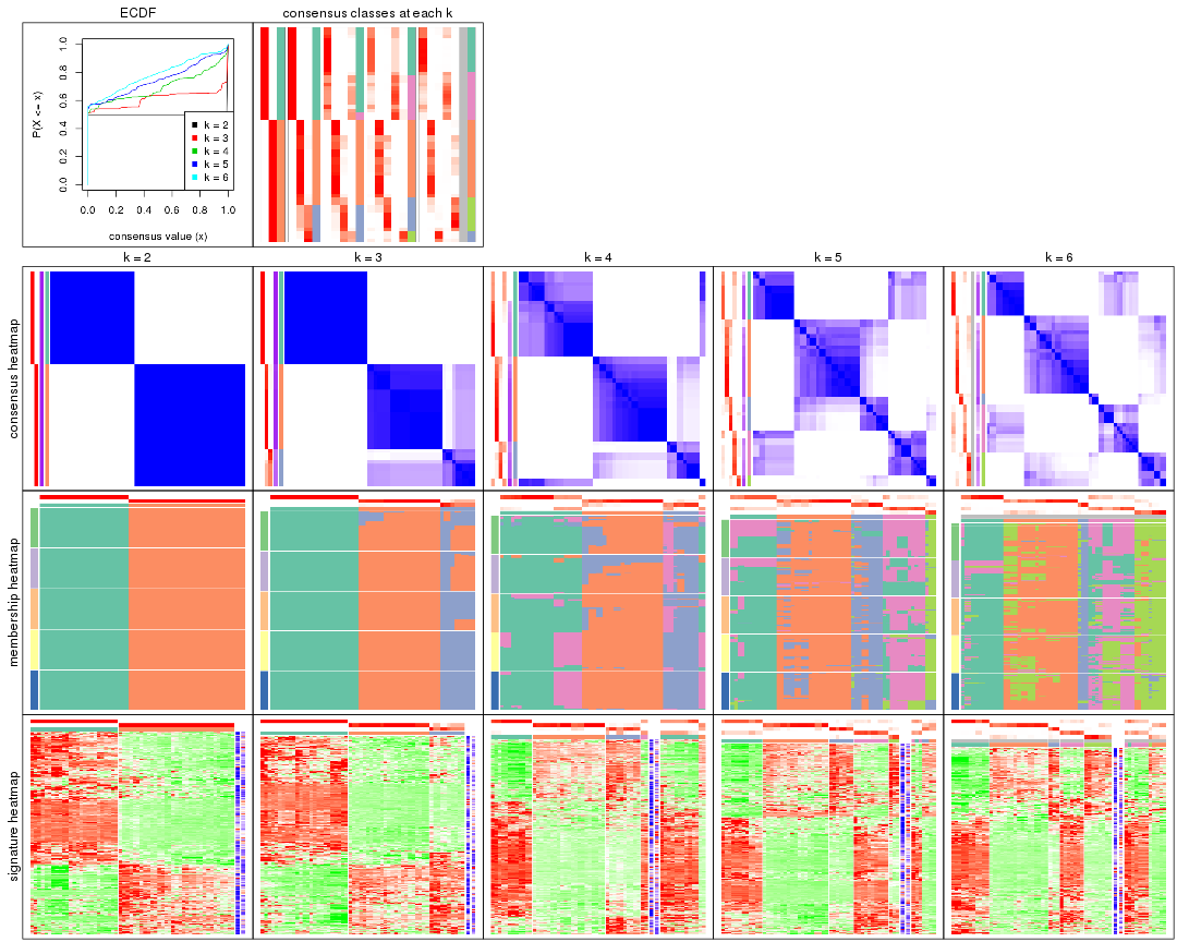
Cumulative distribution function curves of consensus matrix for all methods.
collect_plots(res_list, fun = plot_ecdf)
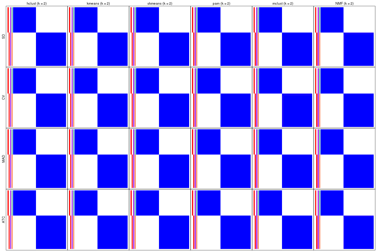
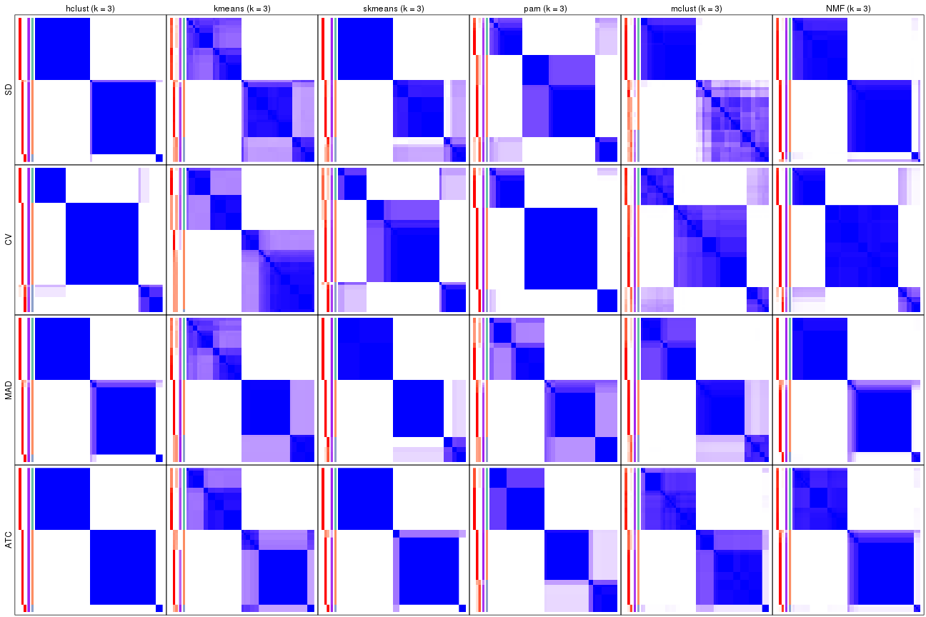
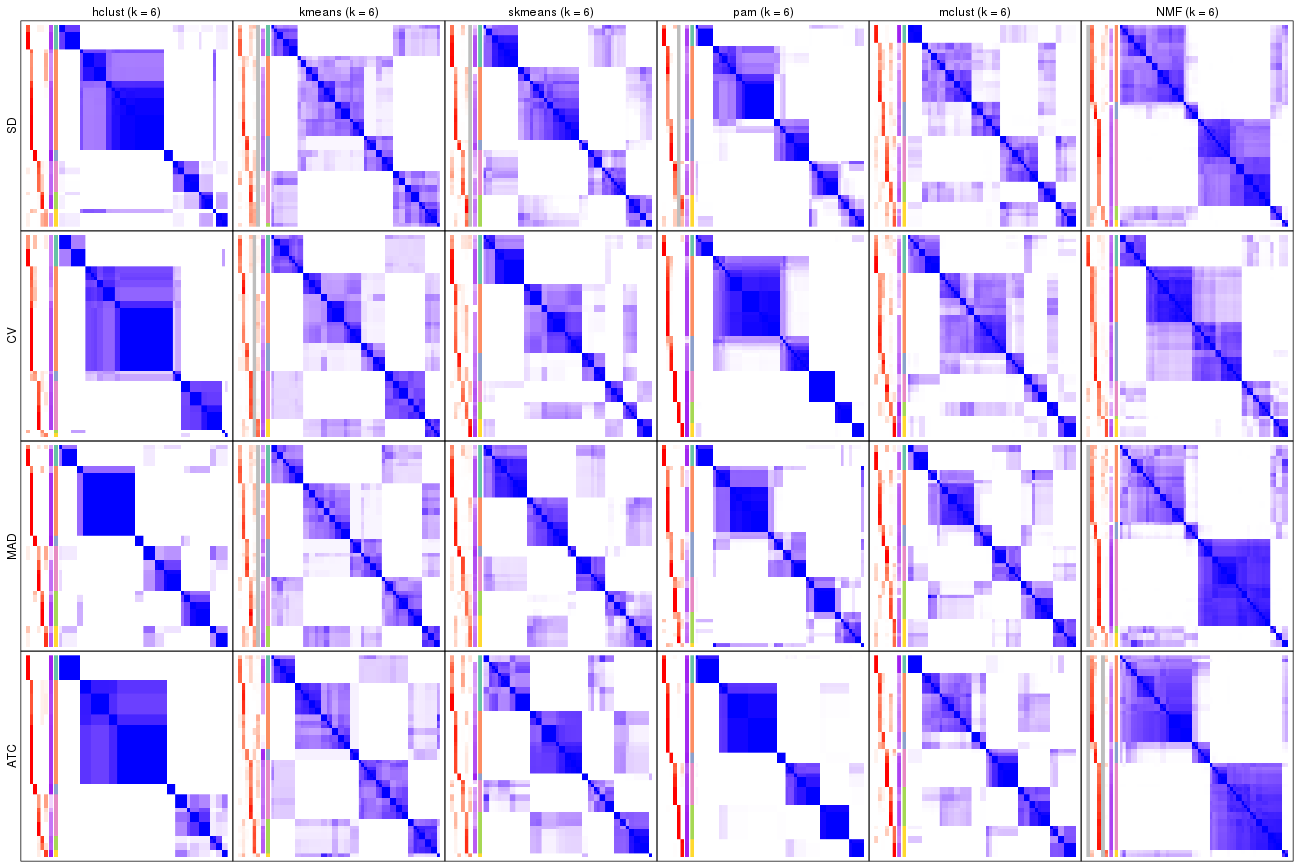
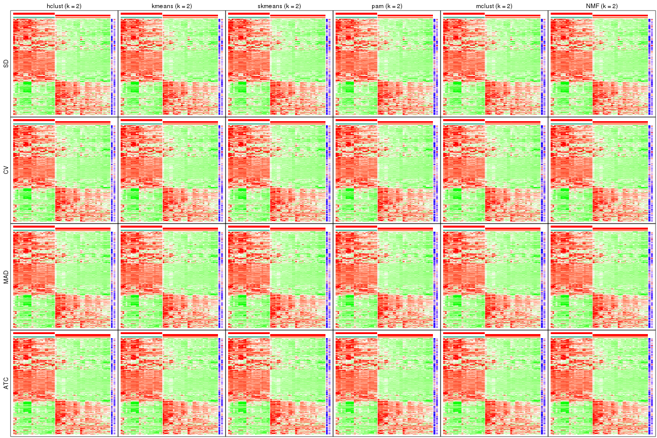
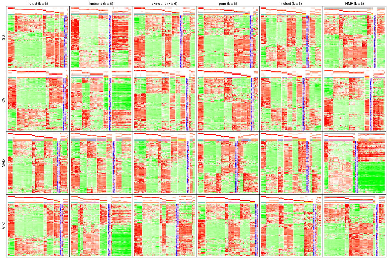
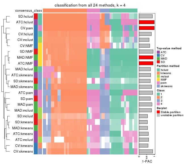
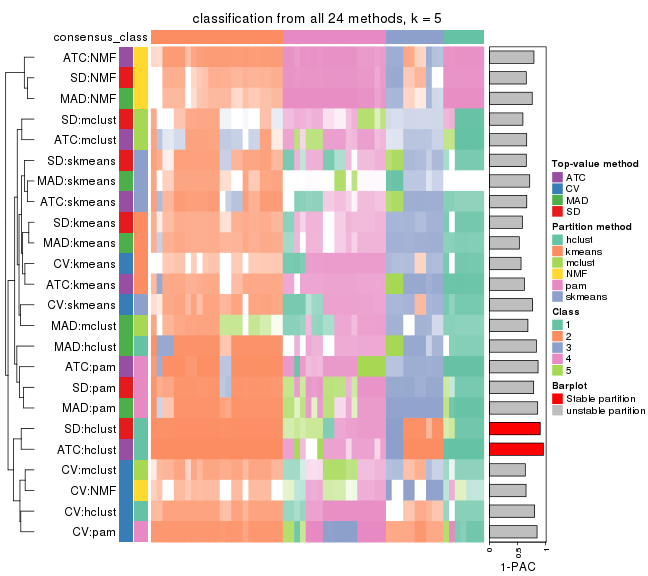
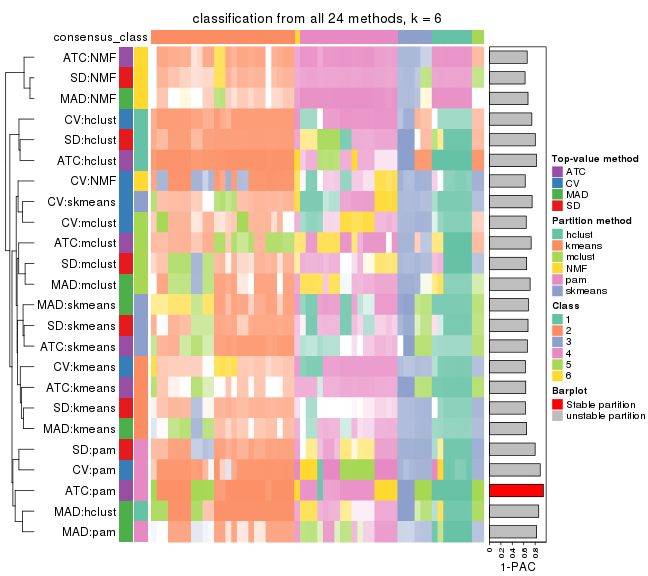
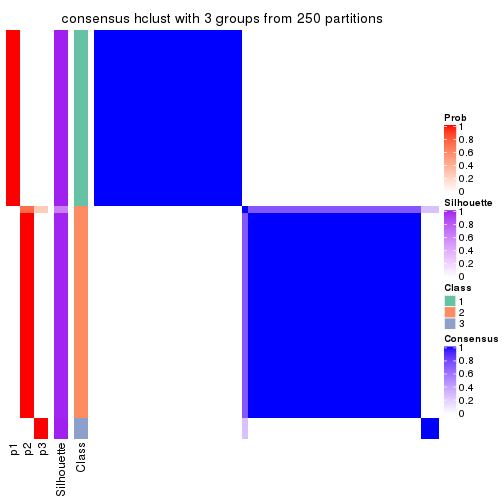
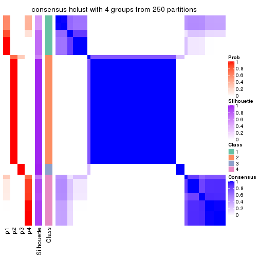
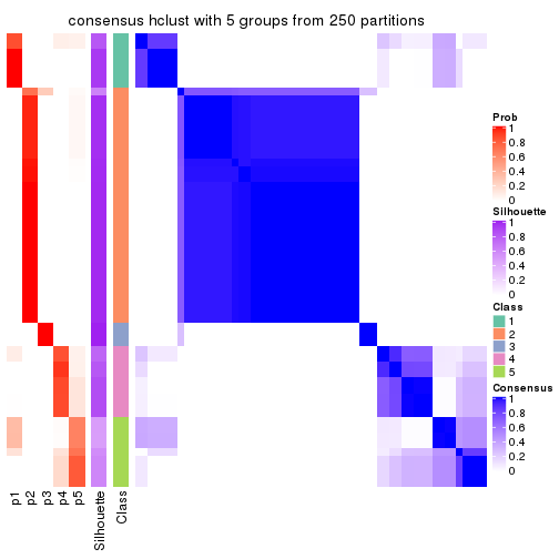
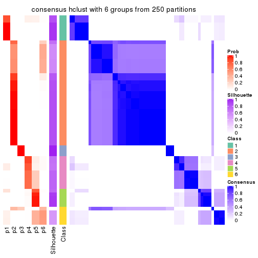
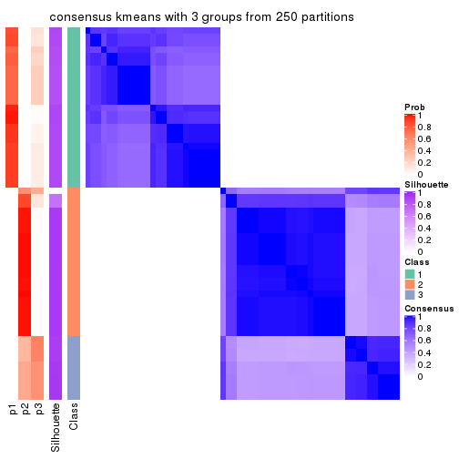
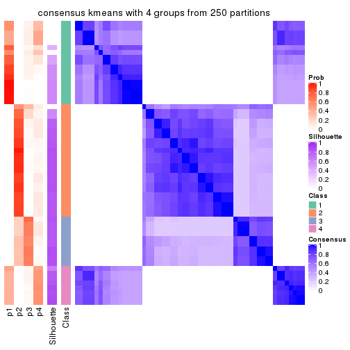
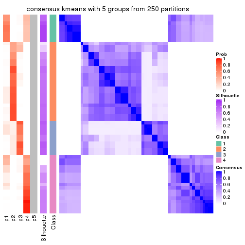
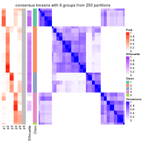
Consensus heatmaps for all methods. (What is a consensus heatmap?)
collect_plots(res_list, k = 2, fun = consensus_heatmap, mc.cores = 4)
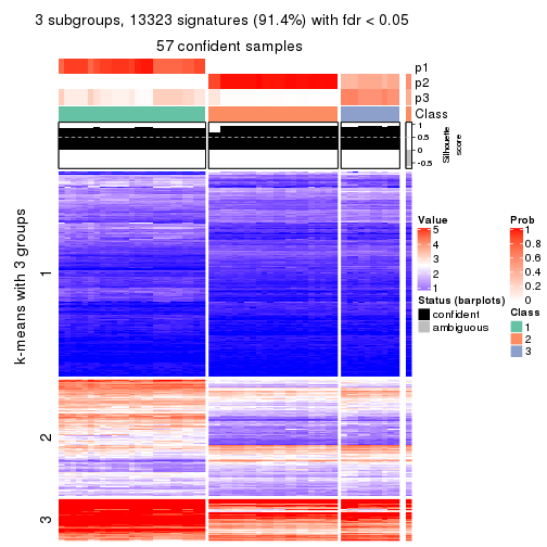
collect_plots(res_list, k = 3, fun = consensus_heatmap, mc.cores = 4)
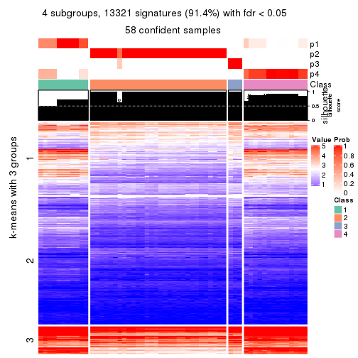
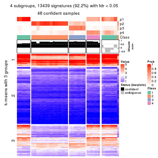
collect_plots(res_list, k = 4, fun = consensus_heatmap, mc.cores = 4)
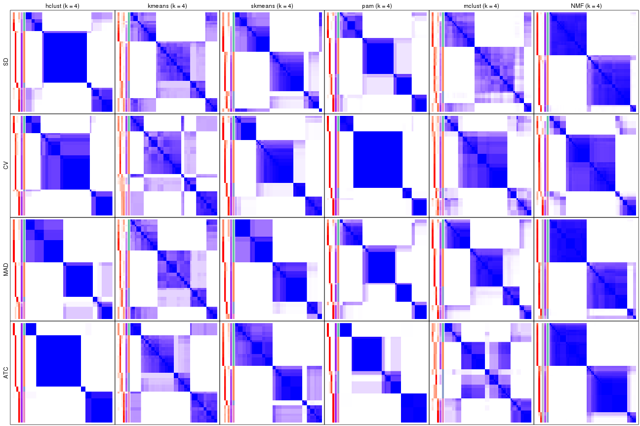
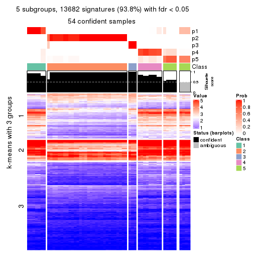
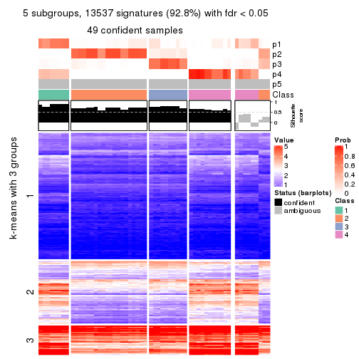
collect_plots(res_list, k = 5, fun = consensus_heatmap, mc.cores = 4)
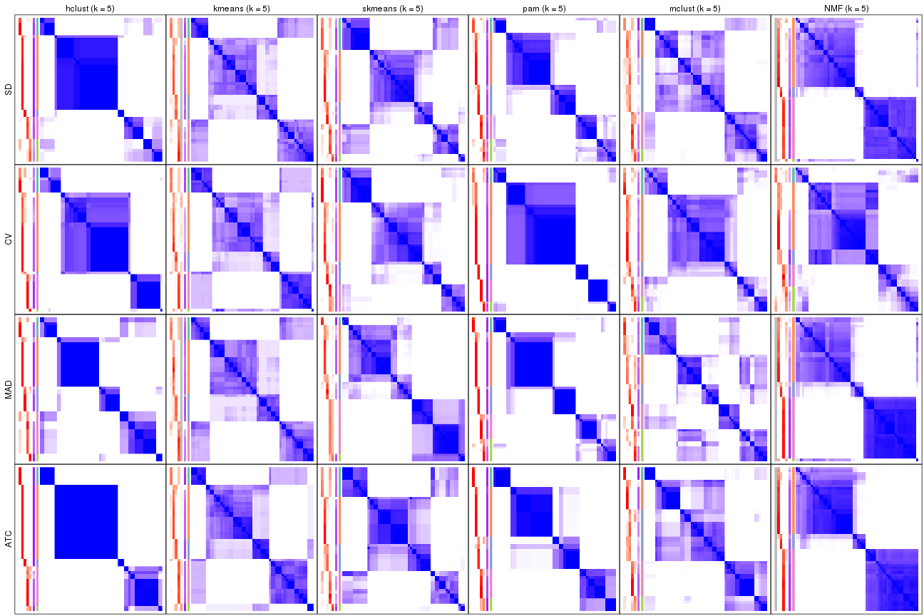
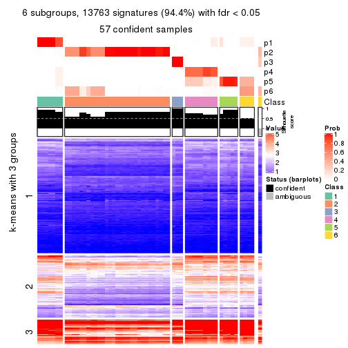
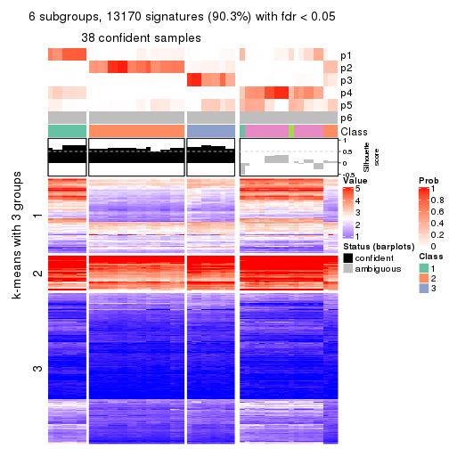
collect_plots(res_list, k = 6, fun = consensus_heatmap, mc.cores = 4)
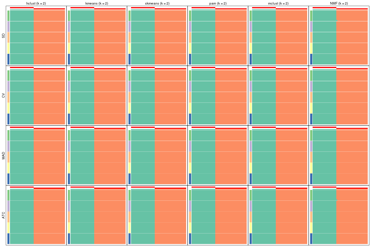
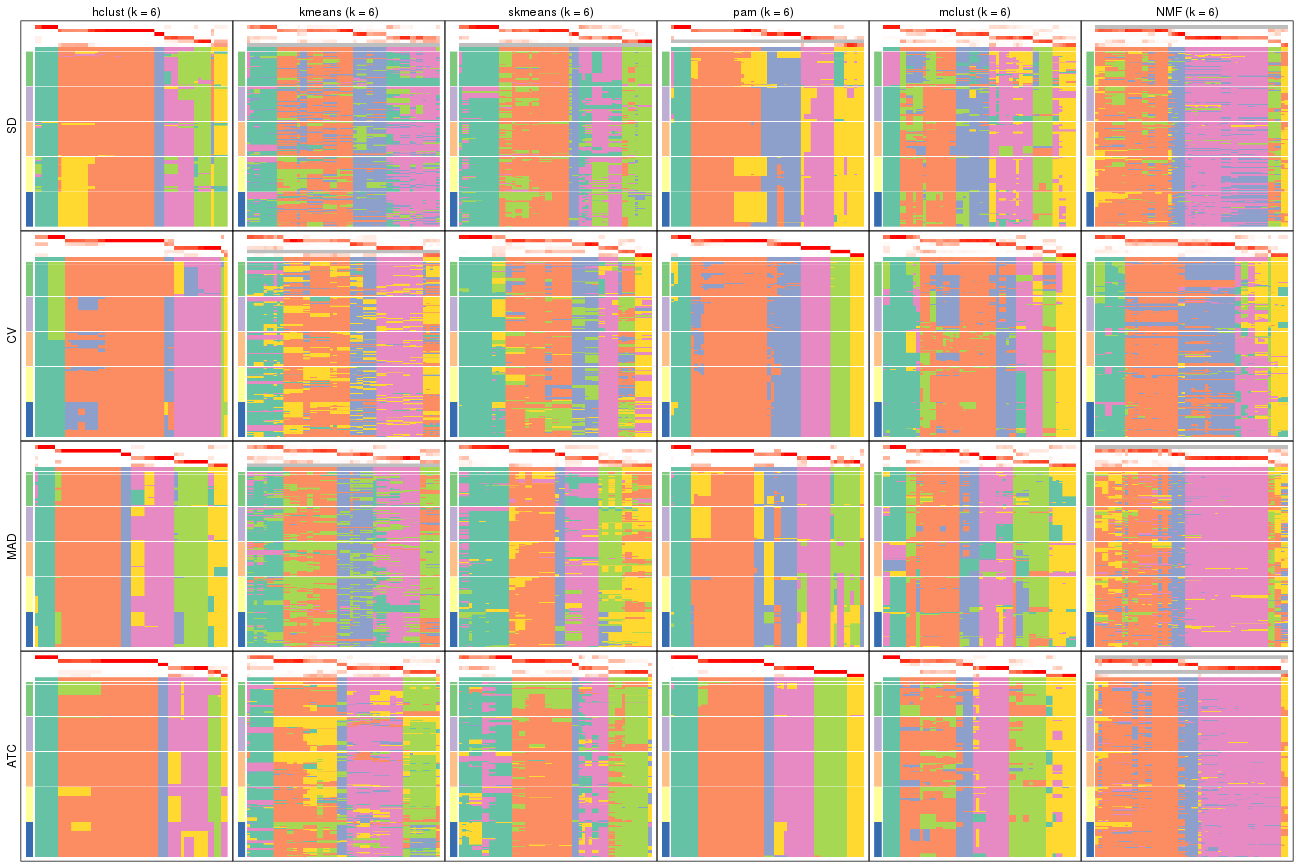
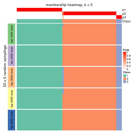
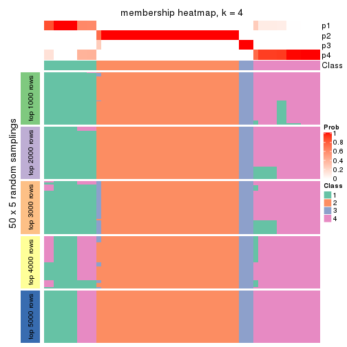
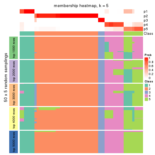
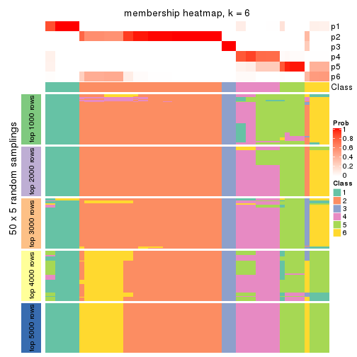
Membership heatmaps for all methods. (What is a membership heatmap?)
collect_plots(res_list, k = 2, fun = membership_heatmap, mc.cores = 4)
collect_plots(res_list, k = 3, fun = membership_heatmap, mc.cores = 4)
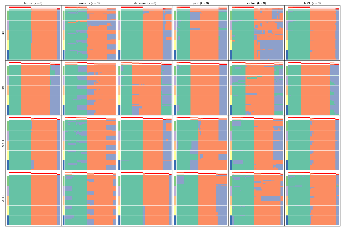
collect_plots(res_list, k = 4, fun = membership_heatmap, mc.cores = 4)
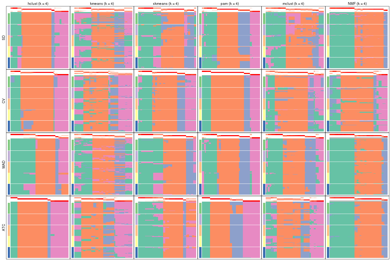
collect_plots(res_list, k = 5, fun = membership_heatmap, mc.cores = 4)
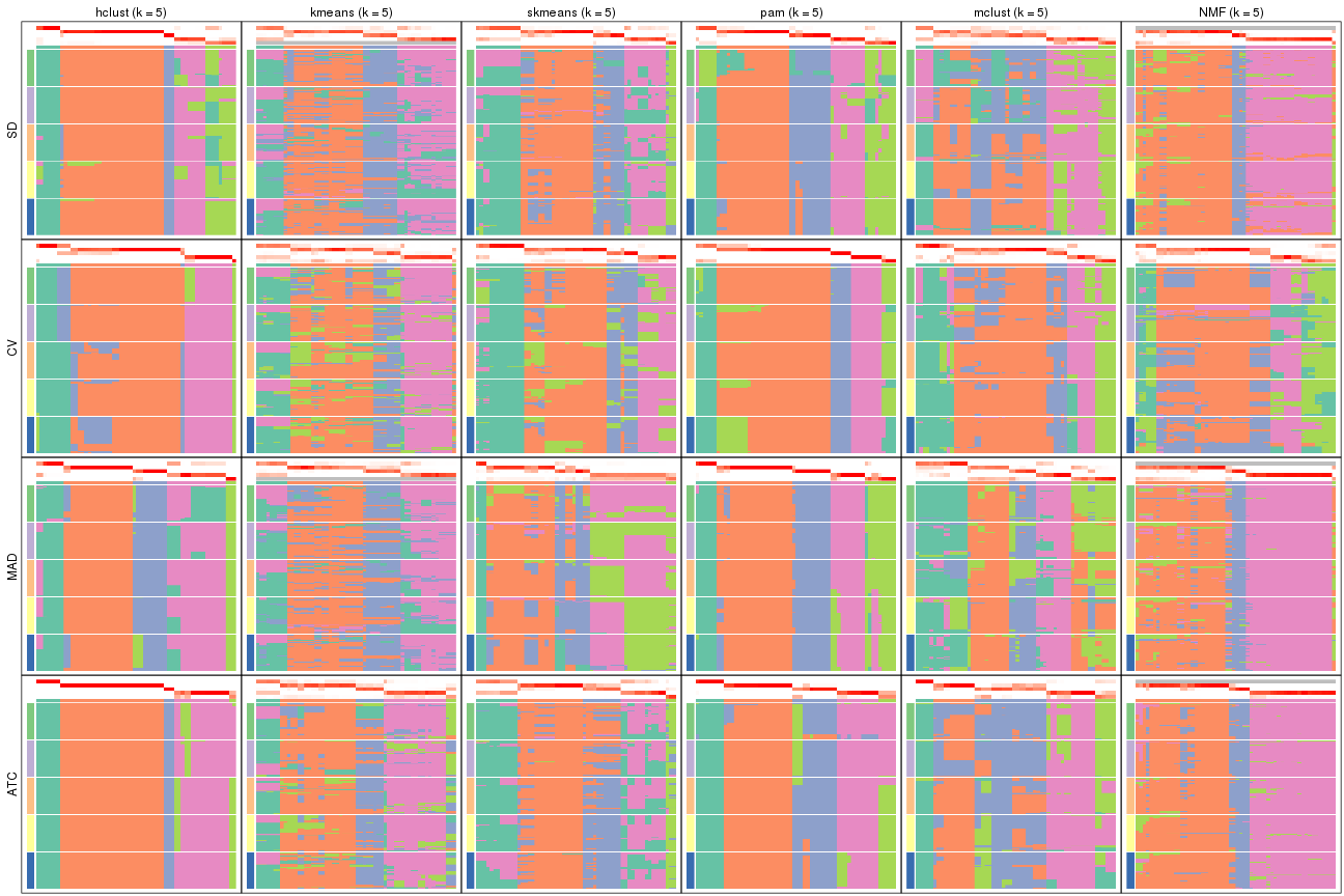
collect_plots(res_list, k = 6, fun = membership_heatmap, mc.cores = 4)
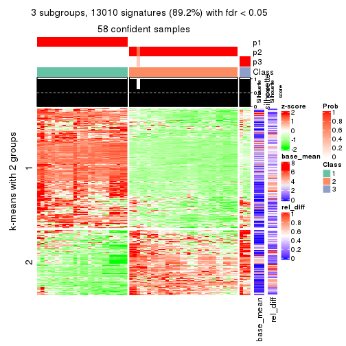
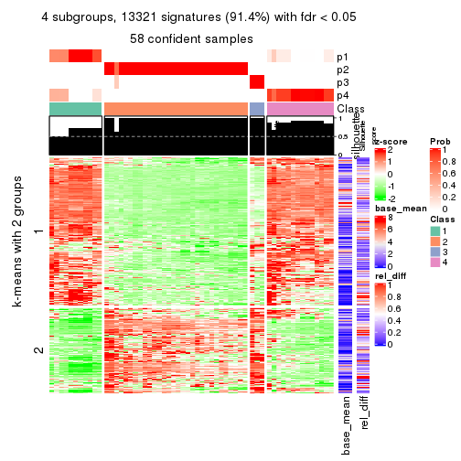
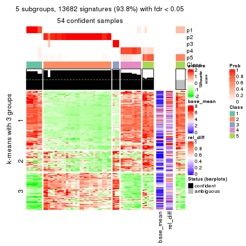
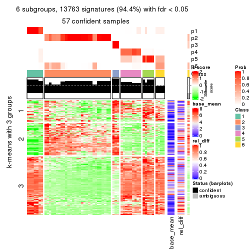
Signature heatmaps for all methods. (What is a signature heatmap?)
Note in following heatmaps, rows are scaled.
collect_plots(res_list, k = 2, fun = get_signatures, mc.cores = 4)
collect_plots(res_list, k = 3, fun = get_signatures, mc.cores = 4)
collect_plots(res_list, k = 4, fun = get_signatures, mc.cores = 4)
collect_plots(res_list, k = 5, fun = get_signatures, mc.cores = 4)
collect_plots(res_list, k = 6, fun = get_signatures, mc.cores = 4)
The statistics used for measuring the stability of consensus partitioning. (How are they defined?)
get_stats(res_list, k = 2)
#>             k 1-PAC mean_silhouette concordance area_increased  Rand Jaccard
#> SD:NMF      2     1           0.999           1            0.5 0.501   0.501
#> CV:NMF      2     1           1.000           1            0.5 0.501   0.501
#> MAD:NMF     2     1           1.000           1            0.5 0.501   0.501
#> ATC:NMF     2     1           0.999           1            0.5 0.501   0.501
#> SD:skmeans  2     1           1.000           1            0.5 0.501   0.501
#> CV:skmeans  2     1           1.000           1            0.5 0.501   0.501
#> MAD:skmeans 2     1           1.000           1            0.5 0.501   0.501
#> ATC:skmeans 2     1           1.000           1            0.5 0.501   0.501
#> SD:mclust   2     1           1.000           1            0.5 0.501   0.501
#> CV:mclust   2     1           0.999           1            0.5 0.501   0.501
#> MAD:mclust  2     1           1.000           1            0.5 0.501   0.501
#> ATC:mclust  2     1           1.000           1            0.5 0.501   0.501
#> SD:kmeans   2     1           1.000           1            0.5 0.501   0.501
#> CV:kmeans   2     1           1.000           1            0.5 0.501   0.501
#> MAD:kmeans  2     1           1.000           1            0.5 0.501   0.501
#> ATC:kmeans  2     1           1.000           1            0.5 0.501   0.501
#> SD:pam      2     1           1.000           1            0.5 0.501   0.501
#> CV:pam      2     1           1.000           1            0.5 0.501   0.501
#> MAD:pam     2     1           1.000           1            0.5 0.501   0.501
#> ATC:pam     2     1           1.000           1            0.5 0.501   0.501
#> SD:hclust   2     1           1.000           1            0.5 0.501   0.501
#> CV:hclust   2     1           1.000           1            0.5 0.501   0.501
#> MAD:hclust  2     1           1.000           1            0.5 0.501   0.501
#> ATC:hclust  2     1           1.000           1            0.5 0.501   0.501
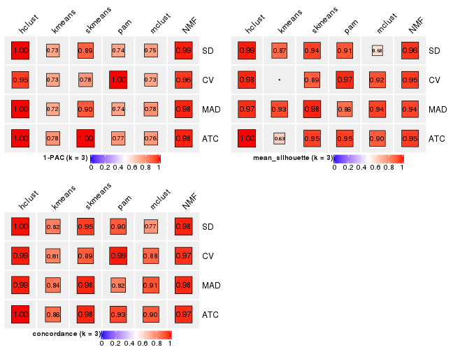
get_stats(res_list, k = 3)
#>             k 1-PAC mean_silhouette concordance area_increased  Rand Jaccard
#> SD:NMF      3 0.987          0.9638       0.982          0.139 0.930   0.860
#> CV:NMF      3 0.957          0.9531       0.966          0.165 0.909   0.819
#> MAD:NMF     3 0.980          0.9398       0.975          0.174 0.930   0.860
#> ATC:NMF     3 0.984          0.9517       0.972          0.136 0.946   0.891
#> SD:skmeans  3 0.888          0.9410       0.949          0.223 0.861   0.722
#> CV:skmeans  3 0.777          0.8885       0.894          0.203 0.906   0.812
#> MAD:skmeans 3 0.902          0.9802       0.981          0.254 0.861   0.722
#> ATC:skmeans 3 1.000          0.9477       0.979          0.144 0.946   0.891
#> SD:mclust   3 0.745          0.5828       0.771          0.222 0.843   0.686
#> CV:mclust   3 0.727          0.9164       0.878          0.187 0.909   0.819
#> MAD:mclust  3 0.780          0.9446       0.914          0.259 0.854   0.708
#> ATC:mclust  3 0.763          0.8967       0.904          0.173 0.946   0.891
#> SD:kmeans   3 0.731          0.8671       0.825          0.243 0.861   0.722
#> CV:kmeans   3 0.732          0.0547       0.811          0.224 0.981   0.961
#> MAD:kmeans  3 0.722          0.9306       0.840          0.240 0.854   0.708
#> ATC:kmeans  3 0.780          0.6314       0.862          0.215 0.946   0.891
#> SD:pam      3 0.735          0.9062       0.899          0.210 0.909   0.819
#> CV:pam      3 1.000          0.9742       0.987          0.178 0.913   0.826
#> MAD:pam     3 0.736          0.8569       0.824          0.242 0.861   0.722
#> ATC:pam     3 0.769          0.9487       0.933          0.284 0.843   0.686
#> SD:hclust   3 1.000          0.9890       0.995          0.117 0.946   0.891
#> CV:hclust   3 0.950          0.9792       0.987          0.180 0.907   0.814
#> MAD:hclust  3 1.000          0.9702       0.987          0.131 0.946   0.891
#> ATC:hclust  3 1.000          1.0000       1.000          0.109 0.946   0.891
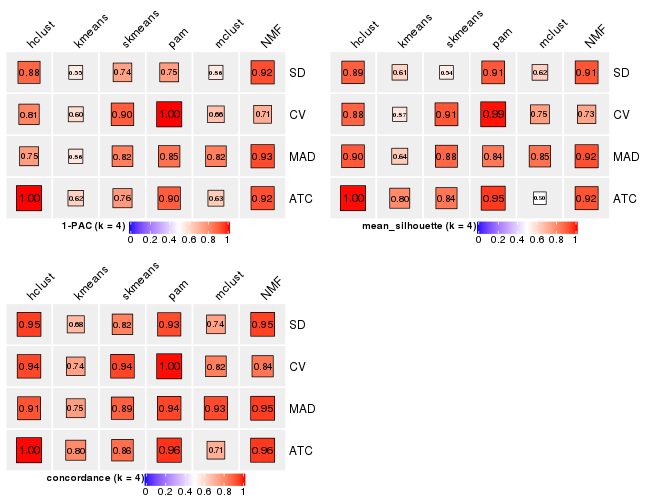
get_stats(res_list, k = 4)
#>             k 1-PAC mean_silhouette concordance area_increased  Rand Jaccard
#> SD:NMF      4 0.924           0.908       0.945         0.0615 1.000   1.000
#> CV:NMF      4 0.708           0.732       0.844         0.0947 0.944   0.868
#> MAD:NMF     4 0.927           0.919       0.951         0.0425 0.962   0.914
#> ATC:NMF     4 0.922           0.916       0.957         0.0718 0.946   0.880
#> SD:skmeans  4 0.741           0.543       0.818         0.1384 0.972   0.923
#> CV:skmeans  4 0.896           0.909       0.940         0.1933 0.864   0.673
#> MAD:skmeans 4 0.825           0.876       0.888         0.0978 0.987   0.965
#> ATC:skmeans 4 0.763           0.842       0.858         0.1506 0.879   0.729
#> SD:mclust   4 0.562           0.624       0.744         0.1387 0.782   0.512
#> CV:mclust   4 0.661           0.752       0.822         0.0923 0.956   0.895
#> MAD:mclust  4 0.823           0.852       0.928         0.1504 0.918   0.768
#> ATC:mclust  4 0.634           0.499       0.706         0.1732 0.746   0.462
#> SD:kmeans   4 0.553           0.613       0.680         0.1091 0.918   0.773
#> CV:kmeans   4 0.595           0.566       0.737         0.1243 0.717   0.471
#> MAD:kmeans  4 0.564           0.637       0.752         0.1286 0.924   0.785
#> ATC:kmeans  4 0.618           0.797       0.797         0.1281 0.803   0.572
#> SD:pam      4 0.750           0.905       0.927         0.2070 0.848   0.628
#> CV:pam      4 1.000           0.993       0.995         0.0584 0.964   0.912
#> MAD:pam     4 0.852           0.839       0.937         0.1929 0.890   0.701
#> ATC:pam     4 0.895           0.955       0.965         0.1243 0.918   0.761
#> SD:hclust   4 0.879           0.893       0.948         0.1520 0.907   0.791
#> CV:hclust   4 0.811           0.885       0.936         0.0767 0.994   0.985
#> MAD:hclust  4 0.755           0.905       0.914         0.1975 0.879   0.729
#> ATC:hclust  4 1.000           0.996       0.998         0.1384 0.924   0.829
get_stats(res_list, k = 5)
#>             k 1-PAC mean_silhouette concordance area_increased  Rand Jaccard
#> SD:NMF      5 0.657           0.694       0.850         0.1070 0.983   0.961
#> CV:NMF      5 0.652           0.357       0.684         0.1106 0.861   0.656
#> MAD:NMF     5 0.762           0.672       0.874         0.0767 0.984   0.961
#> ATC:NMF     5 0.793           0.834       0.901         0.0635 1.000   1.000
#> SD:skmeans  5 0.656           0.680       0.806         0.0758 0.863   0.613
#> CV:skmeans  5 0.768           0.740       0.827         0.0726 0.981   0.934
#> MAD:skmeans 5 0.717           0.374       0.699         0.0932 0.911   0.754
#> ATC:skmeans 5 0.665           0.657       0.780         0.1102 0.888   0.662
#> SD:mclust   5 0.596           0.474       0.640         0.0835 0.791   0.470
#> CV:mclust   5 0.639           0.644       0.816         0.1268 0.881   0.695
#> MAD:mclust  5 0.685           0.619       0.757         0.0762 0.863   0.547
#> ATC:mclust  5 0.663           0.630       0.785         0.0951 0.912   0.689
#> SD:kmeans   5 0.587           0.627       0.705         0.0927 0.913   0.730
#> CV:kmeans   5 0.563           0.542       0.727         0.0827 0.923   0.764
#> MAD:kmeans  5 0.533           0.649       0.715         0.0710 0.913   0.725
#> ATC:kmeans  5 0.624           0.754       0.760         0.0763 0.985   0.948
#> SD:pam      5 0.788           0.838       0.895         0.0657 0.967   0.873
#> CV:pam      5 0.848           0.901       0.926         0.0802 0.982   0.952
#> MAD:pam     5 0.859           0.834       0.932         0.0440 0.967   0.876
#> ATC:pam     5 0.866           0.892       0.905         0.0611 0.964   0.861
#> SD:hclust   5 0.905           0.871       0.915         0.0601 0.944   0.846
#> CV:hclust   5 0.803           0.701       0.898         0.0468 0.981   0.952
#> MAD:hclust  5 0.836           0.743       0.890         0.1267 0.918   0.747
#> ATC:hclust  5 0.962           0.879       0.955         0.0419 0.981   0.948
get_stats(res_list, k = 6)
#>             k 1-PAC mean_silhouette concordance area_increased  Rand Jaccard
#> SD:NMF      6 0.624           0.643       0.757         0.0865 0.912   0.788
#> CV:NMF      6 0.627           0.710       0.773         0.0724 0.790   0.400
#> MAD:NMF     6 0.675           0.575       0.784         0.0817 0.933   0.831
#> ATC:NMF     6 0.661           0.738       0.856         0.0535 0.970   0.925
#> SD:skmeans  6 0.675           0.620       0.742         0.0513 0.985   0.941
#> CV:skmeans  6 0.747           0.679       0.751         0.0434 0.926   0.736
#> MAD:skmeans 6 0.682           0.734       0.770         0.0601 0.831   0.470
#> ATC:skmeans 6 0.666           0.616       0.761         0.0499 0.930   0.734
#> SD:mclust   6 0.649           0.599       0.745         0.0789 0.844   0.470
#> CV:mclust   6 0.644           0.610       0.789         0.0892 0.944   0.802
#> MAD:mclust  6 0.712           0.631       0.771         0.0481 0.897   0.562
#> ATC:mclust  6 0.731           0.730       0.841         0.0746 0.904   0.629
#> SD:kmeans   6 0.631           0.452       0.656         0.0513 0.976   0.917
#> CV:kmeans   6 0.630           0.640       0.692         0.0575 0.935   0.769
#> MAD:kmeans  6 0.649           0.545       0.654         0.0625 0.914   0.691
#> ATC:kmeans  6 0.636           0.538       0.690         0.0588 0.940   0.784
#> SD:pam      6 0.801           0.699       0.816         0.0433 0.979   0.913
#> CV:pam      6 0.890           0.866       0.943         0.1517 0.861   0.617
#> MAD:pam     6 0.826           0.581       0.820         0.0501 0.951   0.800
#> ATC:pam     6 0.945           0.959       0.976         0.0403 0.982   0.919
#> SD:hclust   6 0.803           0.765       0.840         0.0858 0.968   0.901
#> CV:hclust   6 0.742           0.749       0.871         0.0341 0.957   0.888
#> MAD:hclust  6 0.863           0.786       0.901         0.0501 0.956   0.824
#> ATC:hclust  6 0.823           0.845       0.905         0.0685 0.966   0.904
Following heatmap plots the partition for each combination of methods and the lightness correspond to the silhouette scores for samples in each method. On top the consensus subgroup is inferred from all methods by taking the mean silhouette scores as weight.
collect_stats(res_list, k = 2)
collect_stats(res_list, k = 3)
collect_stats(res_list, k = 4)
collect_stats(res_list, k = 5)
collect_stats(res_list, k = 6)
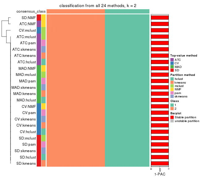
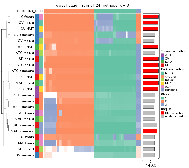
Collect partitions from all methods:
collect_classes(res_list, k = 2)
collect_classes(res_list, k = 3)
collect_classes(res_list, k = 4)
collect_classes(res_list, k = 5)
collect_classes(res_list, k = 6)
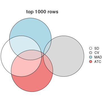
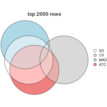
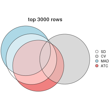
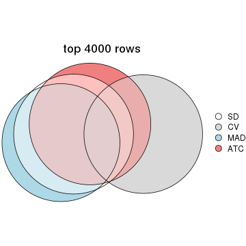
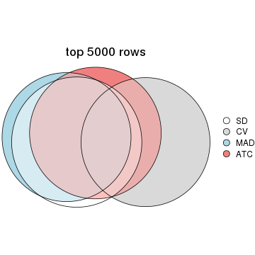
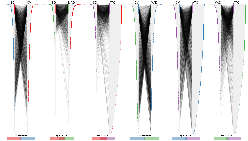
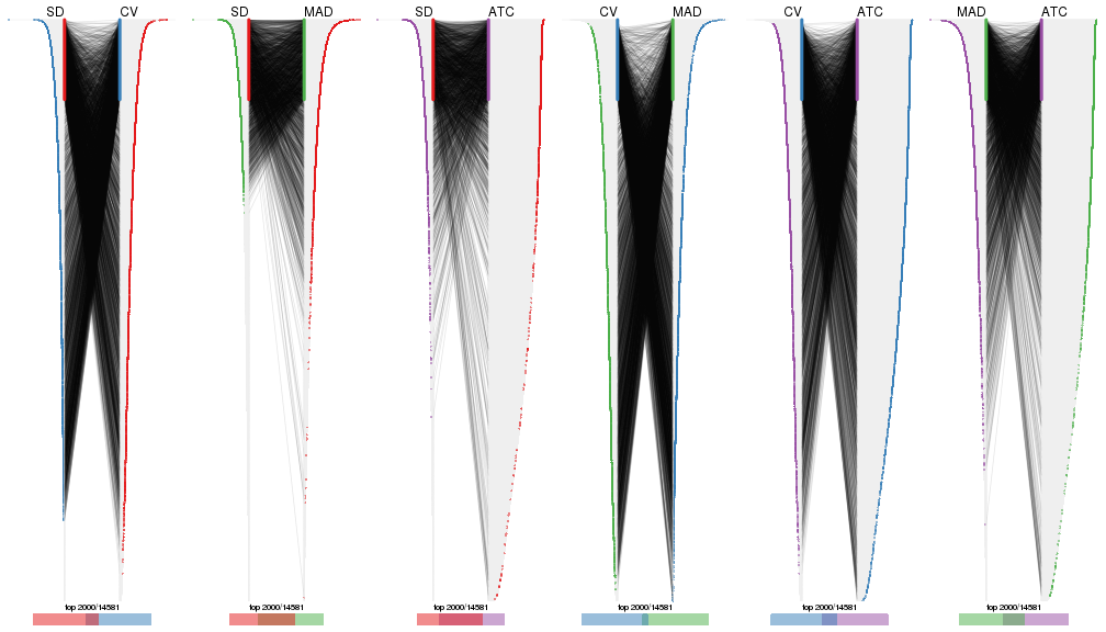
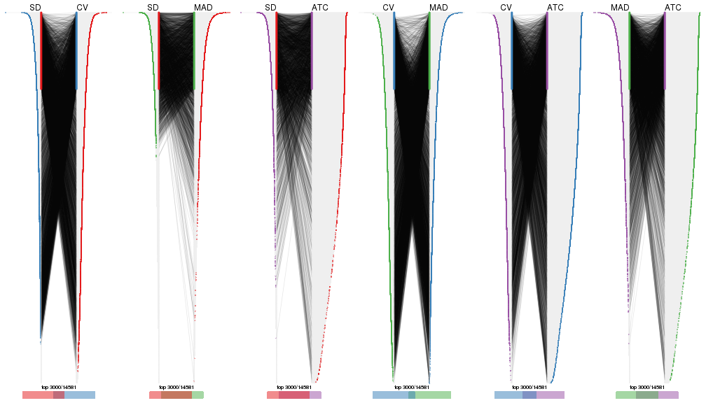
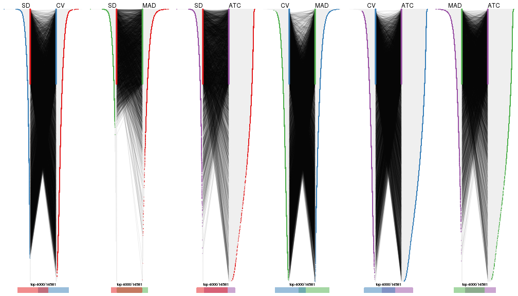
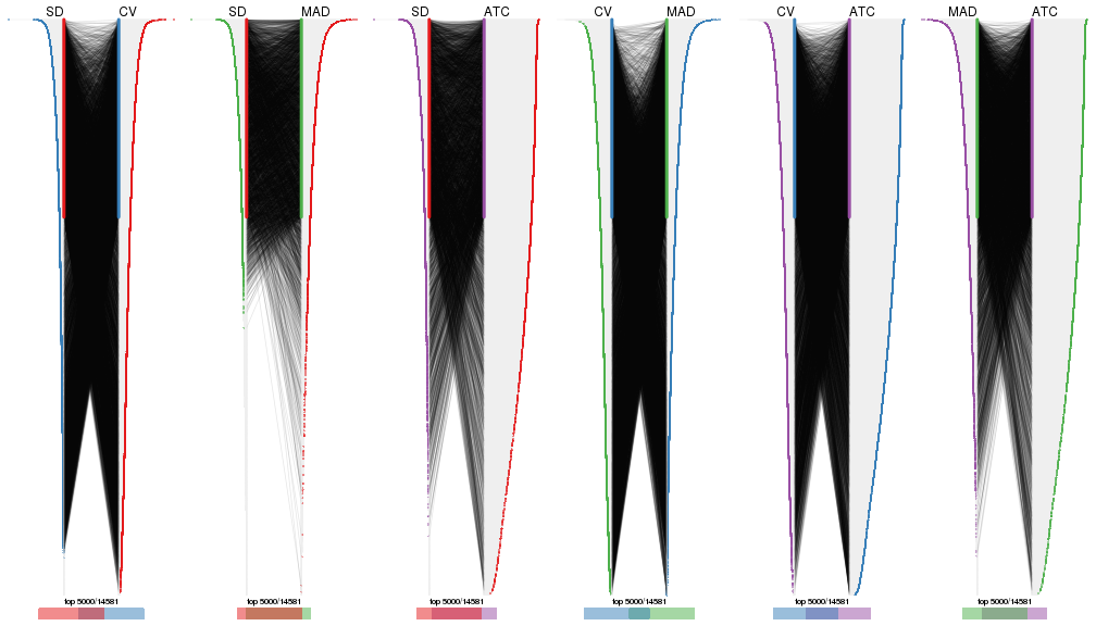
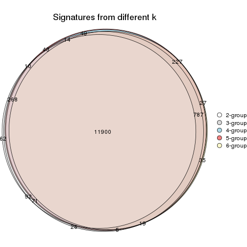
Overlap of top rows from different top-row methods:
top_rows_overlap(res_list, top_n = 1000, method = "euler")
top_rows_overlap(res_list, top_n = 2000, method = "euler")
top_rows_overlap(res_list, top_n = 3000, method = "euler")
top_rows_overlap(res_list, top_n = 4000, method = "euler")
top_rows_overlap(res_list, top_n = 5000, method = "euler")
Also visualize the correspondance of rankings between different top-row methods:
top_rows_overlap(res_list, top_n = 1000, method = "correspondance")
top_rows_overlap(res_list, top_n = 2000, method = "correspondance")
top_rows_overlap(res_list, top_n = 3000, method = "correspondance")
top_rows_overlap(res_list, top_n = 4000, method = "correspondance")
top_rows_overlap(res_list, top_n = 5000, method = "correspondance")
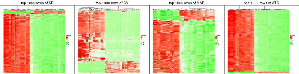
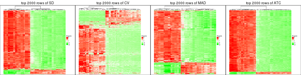
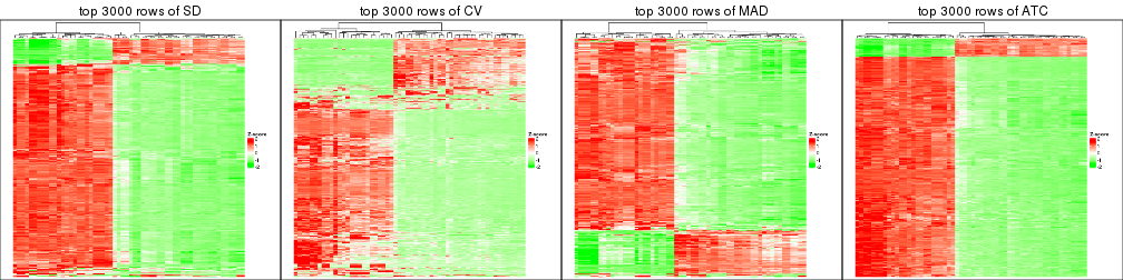
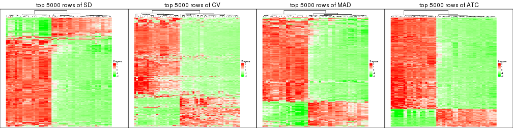
Heatmaps of the top rows:
top_rows_heatmap(res_list, top_n = 1000)
top_rows_heatmap(res_list, top_n = 2000)
top_rows_heatmap(res_list, top_n = 3000)
top_rows_heatmap(res_list, top_n = 4000)
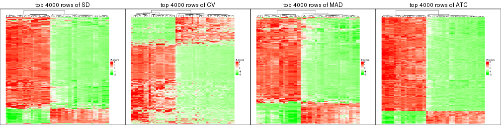
top_rows_heatmap(res_list, top_n = 5000)
The object with results only for a single top-value method and a single partition method can be extracted as:
res = res_list["SD", "hclust"]
# you can also extract it by
# res = res_list["SD:hclust"]
A summary of res and all the functions that can be applied to it:
res
#> A 'ConsensusPartition' object with k = 2, 3, 4, 5, 6.
#>   On a matrix with 14581 rows and 58 columns.
#>   Top rows (1000, 2000, 3000, 4000, 5000) are extracted by 'SD' method.
#>   Subgroups are detected by 'hclust' method.
#>   Performed in total 1250 partitions by row resampling.
#>   Best k for subgroups seems to be 5.
#>
#> Following methods can be applied to this 'ConsensusPartition' object:
#>  [1] "cola_report"             "collect_classes"         "collect_plots"
#>  [4] "collect_stats"           "colnames"                "compare_signatures"
#>  [7] "consensus_heatmap"       "dimension_reduction"     "functional_enrichment"
#> [10] "get_anno_col"            "get_anno"                "get_classes"
#> [13] "get_consensus"           "get_matrix"              "get_membership"
#> [16] "get_param"               "get_signatures"          "get_stats"
#> [19] "is_best_k"               "is_stable_k"             "membership_heatmap"
#> [22] "ncol"                    "nrow"                    "plot_ecdf"
#> [25] "rownames"                "select_partition_number" "show"
#> [28] "suggest_best_k"          "test_to_known_factors"
collect_plots() function collects all the plots made from res for all k (number of partitions)
into one single page to provide an easy and fast comparison between different k.
collect_plots(res)
The plots are:
k and the heatmap of
predicted classes for each k.k.k.k.All the plots in panels can be made by individual functions and they are plotted later in this section.
select_partition_number() produces several plots showing different
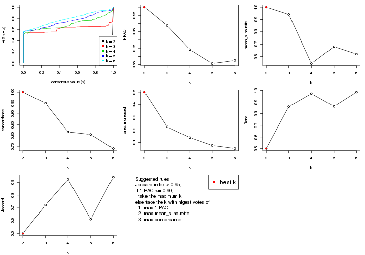
statistics for choosing “optimized” k. There are following statistics:
k;k, the area increased is defined as \(A_k - A_{k-1}\).The detailed explanations of these statistics can be found in the cola vignette.
Generally speaking, lower PAC score, higher mean silhouette score or higher
concordance corresponds to better partition. Rand index and Jaccard index
measure how similar the current partition is compared to partition with k-1.
If they are too similar, we won't accept k is better than k-1.
select_partition_number(res)
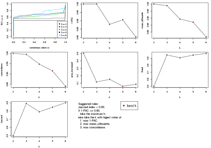
The numeric values for all these statistics can be obtained by get_stats().
get_stats(res)
#>   k 1-PAC mean_silhouette concordance area_increased  Rand Jaccard
#> 2 2 1.000           1.000       1.000         0.4996 0.501   0.501
#> 3 3 1.000           0.989       0.995         0.1173 0.946   0.891
#> 4 4 0.879           0.893       0.948         0.1520 0.907   0.791
#> 5 5 0.905           0.871       0.915         0.0601 0.944   0.846
#> 6 6 0.803           0.765       0.840         0.0858 0.968   0.901
suggest_best_k() suggests the best \(k\) based on these statistics. The rules are as follows:
suggest_best_k(res)
#> [1] 5
#> attr(,"optional")
#> [1] 2 3
There is also optional best \(k\) = 2 3 that is worth to check.
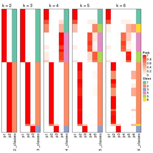
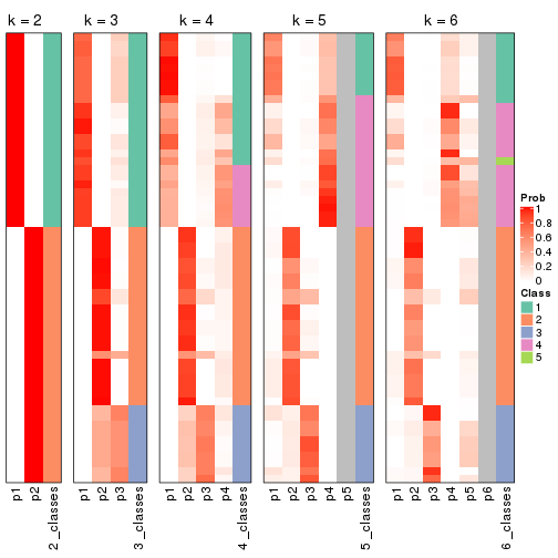
Following shows the table of the partitions (You need to click the show/hide
code output link to see it). The membership matrix (columns with name p*)
is inferred by
clue::cl_consensus()
function with the SE method. Basically the value in the membership matrix
represents the probability to belong to a certain group. The finall class
label for an item is determined with the group with highest probability it
belongs to.
In get_classes() function, the entropy is calculated from the membership
matrix and the silhouette score is calculated from the consensus matrix.
cbind(get_classes(res, k = 2), get_membership(res, k = 2))
#>           class entropy silhouette p1 p2
#> ERR789082     2       0          1  0  1
#> ERR789083     2       0          1  0  1
#> ERR789191     2       0          1  0  1
#> ERR789192     2       0          1  0  1
#> ERR789213     1       0          1  1  0
#> ERR789385     1       0          1  1  0
#> ERR789393     1       0          1  1  0
#> ERR789394     1       0          1  1  0
#> ERR789193     2       0          1  0  1
#> ERR789194     2       0          1  0  1
#> ERR789195     2       0          1  0  1
#> ERR789196     2       0          1  0  1
#> ERR789388     1       0          1  1  0
#> ERR789197     2       0          1  0  1
#> ERR789198     2       0          1  0  1
#> ERR789214     1       0          1  1  0
#> ERR789397     1       0          1  1  0
#> ERR789398     1       0          1  1  0
#> ERR789199     2       0          1  0  1
#> ERR789200     2       0          1  0  1
#> ERR789201     2       0          1  0  1
#> ERR789202     2       0          1  0  1
#> ERR789215     1       0          1  1  0
#> ERR789203     2       0          1  0  1
#> ERR789204     2       0          1  0  1
#> ERR789383     1       0          1  1  0
#> ERR789205     2       0          1  0  1
#> ERR789206     2       0          1  0  1
#> ERR789399     1       0          1  1  0
#> ERR789400     1       0          1  1  0
#> ERR789207     2       0          1  0  1
#> ERR789208     2       0          1  0  1
#> ERR789209     2       0          1  0  1
#> ERR789210     2       0          1  0  1
#> ERR789211     2       0          1  0  1
#> ERR789212     2       0          1  0  1
#> ERR789386     1       0          1  1  0
#> ERR789076     2       0          1  0  1
#> ERR789077     2       0          1  0  1
#> ERR789384     1       0          1  1  0
#> ERR789078     2       0          1  0  1
#> ERR789079     2       0          1  0  1
#> ERR789216     1       0          1  1  0
#> ERR789080     2       0          1  0  1
#> ERR789387     1       0          1  1  0
#> ERR789081     2       0          1  0  1
#> ERR789064     2       0          1  0  1
#> ERR779485     2       0          1  0  1
#> ERR789065     2       0          1  0  1
#> ERR789401     1       0          1  1  0
#> ERR789402     1       0          1  1  0
#> ERR789403     1       0          1  1  0
#> ERR789389     1       0          1  1  0
#> ERR789395     1       0          1  1  0
#> ERR789396     1       0          1  1  0
#> ERR789390     1       0          1  1  0
#> ERR789391     1       0          1  1  0
#> ERR789392     1       0          1  1  0
cbind(get_classes(res, k = 3), get_membership(res, k = 3))
#>           class entropy silhouette p1    p2    p3
#> ERR789082     2   0.000      0.991  0 1.000 0.000
#> ERR789083     2   0.000      0.991  0 1.000 0.000
#> ERR789191     2   0.000      0.991  0 1.000 0.000
#> ERR789192     2   0.000      0.991  0 1.000 0.000
#> ERR789213     1   0.000      1.000  1 0.000 0.000
#> ERR789385     1   0.000      1.000  1 0.000 0.000
#> ERR789393     1   0.000      1.000  1 0.000 0.000
#> ERR789394     1   0.000      1.000  1 0.000 0.000
#> ERR789193     3   0.000      1.000  0 0.000 1.000
#> ERR789194     3   0.000      1.000  0 0.000 1.000
#> ERR789195     2   0.000      0.991  0 1.000 0.000
#> ERR789196     2   0.000      0.991  0 1.000 0.000
#> ERR789388     1   0.000      1.000  1 0.000 0.000
#> ERR789197     2   0.000      0.991  0 1.000 0.000
#> ERR789198     2   0.000      0.991  0 1.000 0.000
#> ERR789214     1   0.000      1.000  1 0.000 0.000
#> ERR789397     1   0.000      1.000  1 0.000 0.000
#> ERR789398     1   0.000      1.000  1 0.000 0.000
#> ERR789199     2   0.000      0.991  0 1.000 0.000
#> ERR789200     2   0.000      0.991  0 1.000 0.000
#> ERR789201     2   0.000      0.991  0 1.000 0.000
#> ERR789202     2   0.000      0.991  0 1.000 0.000
#> ERR789215     1   0.000      1.000  1 0.000 0.000
#> ERR789203     2   0.000      0.991  0 1.000 0.000
#> ERR789204     2   0.000      0.991  0 1.000 0.000
#> ERR789383     1   0.000      1.000  1 0.000 0.000
#> ERR789205     2   0.000      0.991  0 1.000 0.000
#> ERR789206     2   0.000      0.991  0 1.000 0.000
#> ERR789399     1   0.000      1.000  1 0.000 0.000
#> ERR789400     1   0.000      1.000  1 0.000 0.000
#> ERR789207     2   0.000      0.991  0 1.000 0.000
#> ERR789208     2   0.000      0.991  0 1.000 0.000
#> ERR789209     2   0.000      0.991  0 1.000 0.000
#> ERR789210     2   0.000      0.991  0 1.000 0.000
#> ERR789211     2   0.000      0.991  0 1.000 0.000
#> ERR789212     2   0.000      0.991  0 1.000 0.000
#> ERR789386     1   0.000      1.000  1 0.000 0.000
#> ERR789076     2   0.000      0.991  0 1.000 0.000
#> ERR789077     2   0.000      0.991  0 1.000 0.000
#> ERR789384     1   0.000      1.000  1 0.000 0.000
#> ERR789078     2   0.000      0.991  0 1.000 0.000
#> ERR789079     2   0.000      0.991  0 1.000 0.000
#> ERR789216     1   0.000      1.000  1 0.000 0.000
#> ERR789080     2   0.000      0.991  0 1.000 0.000
#> ERR789387     1   0.000      1.000  1 0.000 0.000
#> ERR789081     2   0.000      0.991  0 1.000 0.000
#> ERR789064     2   0.000      0.991  0 1.000 0.000
#> ERR779485     3   0.000      1.000  0 0.000 1.000
#> ERR789065     2   0.529      0.634  0 0.732 0.268
#> ERR789401     1   0.000      1.000  1 0.000 0.000
#> ERR789402     1   0.000      1.000  1 0.000 0.000
#> ERR789403     1   0.000      1.000  1 0.000 0.000
#> ERR789389     1   0.000      1.000  1 0.000 0.000
#> ERR789395     1   0.000      1.000  1 0.000 0.000
#> ERR789396     1   0.000      1.000  1 0.000 0.000
#> ERR789390     1   0.000      1.000  1 0.000 0.000
#> ERR789391     1   0.000      1.000  1 0.000 0.000
#> ERR789392     1   0.000      1.000  1 0.000 0.000
cbind(get_classes(res, k = 4), get_membership(res, k = 4))
#>           class entropy silhouette    p1    p2    p3    p4
#> ERR789082     2  0.0000      0.991 0.000 1.000 0.000 0.000
#> ERR789083     2  0.0000      0.991 0.000 1.000 0.000 0.000
#> ERR789191     2  0.0000      0.991 0.000 1.000 0.000 0.000
#> ERR789192     2  0.0000      0.991 0.000 1.000 0.000 0.000
#> ERR789213     4  0.0000      0.913 0.000 0.000 0.000 1.000
#> ERR789385     4  0.0000      0.913 0.000 0.000 0.000 1.000
#> ERR789393     4  0.0188      0.914 0.004 0.000 0.000 0.996
#> ERR789394     4  0.0188      0.914 0.004 0.000 0.000 0.996
#> ERR789193     3  0.0000      1.000 0.000 0.000 1.000 0.000
#> ERR789194     3  0.0000      1.000 0.000 0.000 1.000 0.000
#> ERR789195     2  0.0000      0.991 0.000 1.000 0.000 0.000
#> ERR789196     2  0.0000      0.991 0.000 1.000 0.000 0.000
#> ERR789388     4  0.0000      0.913 0.000 0.000 0.000 1.000
#> ERR789197     2  0.0000      0.991 0.000 1.000 0.000 0.000
#> ERR789198     2  0.0000      0.991 0.000 1.000 0.000 0.000
#> ERR789214     4  0.0000      0.913 0.000 0.000 0.000 1.000
#> ERR789397     4  0.2216      0.856 0.092 0.000 0.000 0.908
#> ERR789398     4  0.2216      0.856 0.092 0.000 0.000 0.908
#> ERR789199     2  0.0000      0.991 0.000 1.000 0.000 0.000
#> ERR789200     2  0.0000      0.991 0.000 1.000 0.000 0.000
#> ERR789201     2  0.0000      0.991 0.000 1.000 0.000 0.000
#> ERR789202     2  0.0000      0.991 0.000 1.000 0.000 0.000
#> ERR789215     1  0.4855      0.507 0.600 0.000 0.000 0.400
#> ERR789203     2  0.0000      0.991 0.000 1.000 0.000 0.000
#> ERR789204     2  0.0000      0.991 0.000 1.000 0.000 0.000
#> ERR789383     1  0.4855      0.507 0.600 0.000 0.000 0.400
#> ERR789205     2  0.0000      0.991 0.000 1.000 0.000 0.000
#> ERR789206     2  0.0000      0.991 0.000 1.000 0.000 0.000
#> ERR789399     1  0.4843      0.515 0.604 0.000 0.000 0.396
#> ERR789400     1  0.4843      0.515 0.604 0.000 0.000 0.396
#> ERR789207     2  0.0000      0.991 0.000 1.000 0.000 0.000
#> ERR789208     2  0.0000      0.991 0.000 1.000 0.000 0.000
#> ERR789209     2  0.0000      0.991 0.000 1.000 0.000 0.000
#> ERR789210     2  0.0000      0.991 0.000 1.000 0.000 0.000
#> ERR789211     2  0.0000      0.991 0.000 1.000 0.000 0.000
#> ERR789212     2  0.0000      0.991 0.000 1.000 0.000 0.000
#> ERR789386     4  0.2345      0.876 0.100 0.000 0.000 0.900
#> ERR789076     2  0.0000      0.991 0.000 1.000 0.000 0.000
#> ERR789077     2  0.0000      0.991 0.000 1.000 0.000 0.000
#> ERR789384     4  0.2345      0.876 0.100 0.000 0.000 0.900
#> ERR789078     2  0.0000      0.991 0.000 1.000 0.000 0.000
#> ERR789079     2  0.0000      0.991 0.000 1.000 0.000 0.000
#> ERR789216     4  0.2345      0.876 0.100 0.000 0.000 0.900
#> ERR789080     2  0.0000      0.991 0.000 1.000 0.000 0.000
#> ERR789387     4  0.2345      0.876 0.100 0.000 0.000 0.900
#> ERR789081     2  0.0000      0.991 0.000 1.000 0.000 0.000
#> ERR789064     2  0.0000      0.991 0.000 1.000 0.000 0.000
#> ERR779485     3  0.0000      1.000 0.000 0.000 1.000 0.000
#> ERR789065     2  0.4193      0.634 0.000 0.732 0.268 0.000
#> ERR789401     1  0.0000      0.729 1.000 0.000 0.000 0.000
#> ERR789402     1  0.0000      0.729 1.000 0.000 0.000 0.000
#> ERR789403     1  0.0000      0.729 1.000 0.000 0.000 0.000
#> ERR789389     4  0.4164      0.673 0.264 0.000 0.000 0.736
#> ERR789395     1  0.0000      0.729 1.000 0.000 0.000 0.000
#> ERR789396     1  0.0000      0.729 1.000 0.000 0.000 0.000
#> ERR789390     1  0.3123      0.725 0.844 0.000 0.000 0.156
#> ERR789391     1  0.3123      0.725 0.844 0.000 0.000 0.156
#> ERR789392     4  0.0188      0.914 0.004 0.000 0.000 0.996
cbind(get_classes(res, k = 5), get_membership(res, k = 5))
#>           class entropy silhouette    p1    p2    p3    p4    p5
#> ERR789082     2  0.0000      0.979 0.000 1.000 0.000 0.000 0.000
#> ERR789083     2  0.0000      0.979 0.000 1.000 0.000 0.000 0.000
#> ERR789191     2  0.0000      0.979 0.000 1.000 0.000 0.000 0.000
#> ERR789192     2  0.0000      0.979 0.000 1.000 0.000 0.000 0.000
#> ERR789213     4  0.2471      0.856 0.000 0.000 0.000 0.864 0.136
#> ERR789385     4  0.2471      0.856 0.000 0.000 0.000 0.864 0.136
#> ERR789393     4  0.2629      0.857 0.004 0.000 0.000 0.860 0.136
#> ERR789394     4  0.2629      0.857 0.004 0.000 0.000 0.860 0.136
#> ERR789193     3  0.0000      1.000 0.000 0.000 1.000 0.000 0.000
#> ERR789194     3  0.0000      1.000 0.000 0.000 1.000 0.000 0.000
#> ERR789195     2  0.1043      0.965 0.000 0.960 0.000 0.000 0.040
#> ERR789196     2  0.1043      0.965 0.000 0.960 0.000 0.000 0.040
#> ERR789388     4  0.1671      0.813 0.000 0.000 0.000 0.924 0.076
#> ERR789197     2  0.1043      0.965 0.000 0.960 0.000 0.000 0.040
#> ERR789198     2  0.1043      0.965 0.000 0.960 0.000 0.000 0.040
#> ERR789214     4  0.1671      0.813 0.000 0.000 0.000 0.924 0.076
#> ERR789397     4  0.3471      0.753 0.092 0.000 0.000 0.836 0.072
#> ERR789398     4  0.3471      0.753 0.092 0.000 0.000 0.836 0.072
#> ERR789199     2  0.0000      0.979 0.000 1.000 0.000 0.000 0.000
#> ERR789200     2  0.0000      0.979 0.000 1.000 0.000 0.000 0.000
#> ERR789201     2  0.0404      0.975 0.000 0.988 0.000 0.000 0.012
#> ERR789202     2  0.0404      0.975 0.000 0.988 0.000 0.000 0.012
#> ERR789215     5  0.4570      0.487 0.348 0.000 0.000 0.020 0.632
#> ERR789203     2  0.1043      0.965 0.000 0.960 0.000 0.000 0.040
#> ERR789204     2  0.1043      0.965 0.000 0.960 0.000 0.000 0.040
#> ERR789383     5  0.4570      0.487 0.348 0.000 0.000 0.020 0.632
#> ERR789205     2  0.1043      0.965 0.000 0.960 0.000 0.000 0.040
#> ERR789206     2  0.1043      0.965 0.000 0.960 0.000 0.000 0.040
#> ERR789399     5  0.4497      0.484 0.352 0.000 0.000 0.016 0.632
#> ERR789400     5  0.4497      0.484 0.352 0.000 0.000 0.016 0.632
#> ERR789207     2  0.0000      0.979 0.000 1.000 0.000 0.000 0.000
#> ERR789208     2  0.0000      0.979 0.000 1.000 0.000 0.000 0.000
#> ERR789209     2  0.0000      0.979 0.000 1.000 0.000 0.000 0.000
#> ERR789210     2  0.0000      0.979 0.000 1.000 0.000 0.000 0.000
#> ERR789211     2  0.0000      0.979 0.000 1.000 0.000 0.000 0.000
#> ERR789212     2  0.0000      0.979 0.000 1.000 0.000 0.000 0.000
#> ERR789386     5  0.3074      0.601 0.000 0.000 0.000 0.196 0.804
#> ERR789076     2  0.0510      0.974 0.000 0.984 0.000 0.000 0.016
#> ERR789077     2  0.0000      0.979 0.000 1.000 0.000 0.000 0.000
#> ERR789384     5  0.3074      0.601 0.000 0.000 0.000 0.196 0.804
#> ERR789078     2  0.0000      0.979 0.000 1.000 0.000 0.000 0.000
#> ERR789079     2  0.0000      0.979 0.000 1.000 0.000 0.000 0.000
#> ERR789216     5  0.3074      0.601 0.000 0.000 0.000 0.196 0.804
#> ERR789080     2  0.0000      0.979 0.000 1.000 0.000 0.000 0.000
#> ERR789387     5  0.3074      0.601 0.000 0.000 0.000 0.196 0.804
#> ERR789081     2  0.0000      0.979 0.000 1.000 0.000 0.000 0.000
#> ERR789064     2  0.0000      0.979 0.000 1.000 0.000 0.000 0.000
#> ERR779485     3  0.0000      1.000 0.000 0.000 1.000 0.000 0.000
#> ERR789065     2  0.4350      0.620 0.000 0.704 0.268 0.000 0.028
#> ERR789401     1  0.0000      0.931 1.000 0.000 0.000 0.000 0.000
#> ERR789402     1  0.0000      0.931 1.000 0.000 0.000 0.000 0.000
#> ERR789403     1  0.0000      0.931 1.000 0.000 0.000 0.000 0.000
#> ERR789389     5  0.5126      0.569 0.152 0.000 0.000 0.152 0.696
#> ERR789395     1  0.0000      0.931 1.000 0.000 0.000 0.000 0.000
#> ERR789396     1  0.0000      0.931 1.000 0.000 0.000 0.000 0.000
#> ERR789390     1  0.3359      0.813 0.844 0.000 0.000 0.084 0.072
#> ERR789391     1  0.3359      0.813 0.844 0.000 0.000 0.084 0.072
#> ERR789392     4  0.2629      0.857 0.004 0.000 0.000 0.860 0.136
cbind(get_classes(res, k = 6), get_membership(res, k = 6))
#>           class entropy silhouette    p1    p2    p3    p4    p5    p6
#> ERR789082     2  0.0000      0.847 0.000 1.000 0.000 0.000 0.000 0.000
#> ERR789083     2  0.0000      0.847 0.000 1.000 0.000 0.000 0.000 0.000
#> ERR789191     2  0.0000      0.847 0.000 1.000 0.000 0.000 0.000 0.000
#> ERR789192     2  0.0000      0.847 0.000 1.000 0.000 0.000 0.000 0.000
#> ERR789213     4  0.3221      0.757 0.000 0.000 0.000 0.736 0.264 0.000
#> ERR789385     4  0.3221      0.757 0.000 0.000 0.000 0.736 0.264 0.000
#> ERR789393     4  0.3360      0.759 0.004 0.000 0.000 0.732 0.264 0.000
#> ERR789394     4  0.3360      0.759 0.004 0.000 0.000 0.732 0.264 0.000
#> ERR789193     3  0.0000      1.000 0.000 0.000 1.000 0.000 0.000 0.000
#> ERR789194     3  0.0000      1.000 0.000 0.000 1.000 0.000 0.000 0.000
#> ERR789195     2  0.3804      0.591 0.000 0.576 0.000 0.000 0.000 0.424
#> ERR789196     2  0.3804      0.591 0.000 0.576 0.000 0.000 0.000 0.424
#> ERR789388     4  0.2361      0.704 0.000 0.000 0.000 0.884 0.088 0.028
#> ERR789197     2  0.3804      0.591 0.000 0.576 0.000 0.000 0.000 0.424
#> ERR789198     2  0.3804      0.591 0.000 0.576 0.000 0.000 0.000 0.424
#> ERR789214     4  0.2361      0.704 0.000 0.000 0.000 0.884 0.088 0.028
#> ERR789397     4  0.3748      0.689 0.092 0.000 0.000 0.812 0.068 0.028
#> ERR789398     4  0.3748      0.689 0.092 0.000 0.000 0.812 0.068 0.028
#> ERR789199     2  0.0146      0.846 0.000 0.996 0.000 0.000 0.000 0.004
#> ERR789200     2  0.0146      0.846 0.000 0.996 0.000 0.000 0.000 0.004
#> ERR789201     2  0.1765      0.811 0.000 0.904 0.000 0.000 0.000 0.096
#> ERR789202     2  0.1765      0.811 0.000 0.904 0.000 0.000 0.000 0.096
#> ERR789215     6  0.5122      0.514 0.072 0.000 0.000 0.004 0.404 0.520
#> ERR789203     2  0.3828      0.578 0.000 0.560 0.000 0.000 0.000 0.440
#> ERR789204     2  0.3828      0.578 0.000 0.560 0.000 0.000 0.000 0.440
#> ERR789383     6  0.5122      0.514 0.072 0.000 0.000 0.004 0.404 0.520
#> ERR789205     2  0.3828      0.578 0.000 0.560 0.000 0.000 0.000 0.440
#> ERR789206     2  0.3828      0.578 0.000 0.560 0.000 0.000 0.000 0.440
#> ERR789399     6  0.5207      0.514 0.080 0.000 0.000 0.004 0.404 0.512
#> ERR789400     6  0.5207      0.514 0.080 0.000 0.000 0.004 0.404 0.512
#> ERR789207     2  0.0000      0.847 0.000 1.000 0.000 0.000 0.000 0.000
#> ERR789208     2  0.0000      0.847 0.000 1.000 0.000 0.000 0.000 0.000
#> ERR789209     2  0.0000      0.847 0.000 1.000 0.000 0.000 0.000 0.000
#> ERR789210     2  0.0000      0.847 0.000 1.000 0.000 0.000 0.000 0.000
#> ERR789211     2  0.0000      0.847 0.000 1.000 0.000 0.000 0.000 0.000
#> ERR789212     2  0.0000      0.847 0.000 1.000 0.000 0.000 0.000 0.000
#> ERR789386     5  0.0547      0.933 0.000 0.000 0.000 0.020 0.980 0.000
#> ERR789076     2  0.3101      0.718 0.000 0.756 0.000 0.000 0.000 0.244
#> ERR789077     2  0.0547      0.843 0.000 0.980 0.000 0.000 0.000 0.020
#> ERR789384     5  0.0865      0.920 0.000 0.000 0.000 0.036 0.964 0.000
#> ERR789078     2  0.0547      0.843 0.000 0.980 0.000 0.000 0.000 0.020
#> ERR789079     2  0.0146      0.846 0.000 0.996 0.000 0.000 0.000 0.004
#> ERR789216     5  0.0547      0.933 0.000 0.000 0.000 0.020 0.980 0.000
#> ERR789080     2  0.0146      0.846 0.000 0.996 0.000 0.000 0.000 0.004
#> ERR789387     5  0.0547      0.933 0.000 0.000 0.000 0.020 0.980 0.000
#> ERR789081     2  0.0146      0.846 0.000 0.996 0.000 0.000 0.000 0.004
#> ERR789064     2  0.0547      0.843 0.000 0.980 0.000 0.000 0.000 0.020
#> ERR779485     3  0.0000      1.000 0.000 0.000 1.000 0.000 0.000 0.000
#> ERR789065     6  0.6075     -0.330 0.000 0.360 0.268 0.000 0.000 0.372
#> ERR789401     1  0.0000      0.939 1.000 0.000 0.000 0.000 0.000 0.000
#> ERR789402     1  0.0000      0.939 1.000 0.000 0.000 0.000 0.000 0.000
#> ERR789403     1  0.0000      0.939 1.000 0.000 0.000 0.000 0.000 0.000
#> ERR789389     5  0.3338      0.743 0.152 0.000 0.000 0.024 0.812 0.012
#> ERR789395     1  0.0000      0.939 1.000 0.000 0.000 0.000 0.000 0.000
#> ERR789396     1  0.0000      0.939 1.000 0.000 0.000 0.000 0.000 0.000
#> ERR789390     1  0.3208      0.843 0.844 0.000 0.000 0.076 0.068 0.012
#> ERR789391     1  0.3208      0.843 0.844 0.000 0.000 0.076 0.068 0.012
#> ERR789392     4  0.3360      0.759 0.004 0.000 0.000 0.732 0.264 0.000
Heatmaps for the consensus matrix. It visualizes the probability of two samples to be in a same group.
consensus_heatmap(res, k = 2)

consensus_heatmap(res, k = 3)
consensus_heatmap(res, k = 4)
consensus_heatmap(res, k = 5)
consensus_heatmap(res, k = 6)
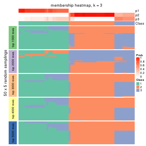
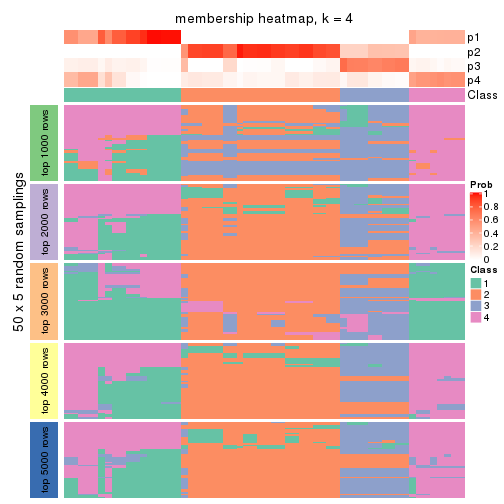
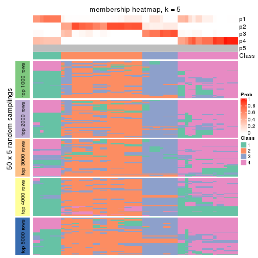
Heatmaps for the membership of samples in all partitions to see how consistent they are:
membership_heatmap(res, k = 2)

membership_heatmap(res, k = 3)
membership_heatmap(res, k = 4)
membership_heatmap(res, k = 5)
membership_heatmap(res, k = 6)
As soon as we have had the classes for columns, we can look for signatures which are significantly different between classes which can be candidate marks for certain classes. Following are the heatmaps for signatures.
Signature heatmaps where rows are scaled:
get_signatures(res, k = 2)

get_signatures(res, k = 3)
get_signatures(res, k = 4)
get_signatures(res, k = 5)
get_signatures(res, k = 6)
Signature heatmaps where rows are not scaled:
get_signatures(res, k = 2, scale_rows = FALSE)

get_signatures(res, k = 3, scale_rows = FALSE)

get_signatures(res, k = 4, scale_rows = FALSE)
get_signatures(res, k = 5, scale_rows = FALSE)
get_signatures(res, k = 6, scale_rows = FALSE)
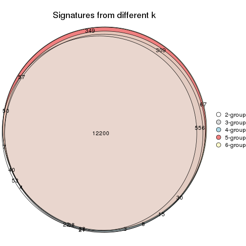
Compare the overlap of signatures from different k:
compare_signatures(res)
get_signature() returns a data frame invisibly. TO get the list of signatures, the function
call should be assigned to a variable explicitly. In following code, if plot argument is set
to FALSE, no heatmap is plotted while only the differential analysis is performed.
# code only for demonstration
tb = get_signature(res, k = ..., plot = FALSE)
An example of the output of tb is:
#>   which_row         fdr    mean_1    mean_2 scaled_mean_1 scaled_mean_2 km
#> 1        38 0.042760348  8.373488  9.131774    -0.5533452     0.5164555  1
#> 2        40 0.018707592  7.106213  8.469186    -0.6173731     0.5762149  1
#> 3        55 0.019134737 10.221463 11.207825    -0.6159697     0.5749050  1
#> 4        59 0.006059896  5.921854  7.869574    -0.6899429     0.6439467  1
#> 5        60 0.018055526  8.928898 10.211722    -0.6204761     0.5791110  1
#> 6        98 0.009384629 15.714769 14.887706     0.6635654    -0.6193277  2
...
The columns in tb are:
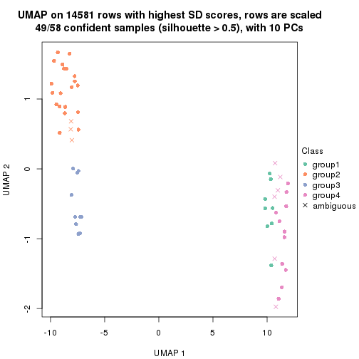
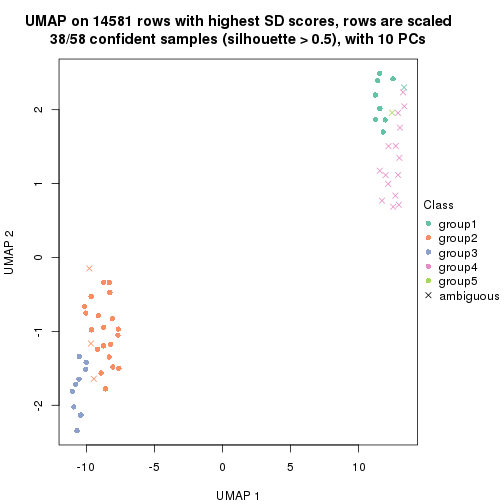
which_row: row indices corresponding to the input matrix.fdr: FDR for the differential test. mean_x: The mean value in group x.scaled_mean_x: The mean value in group x after rows are scaled.km: Row groups if k-means clustering is applied to rows.UMAP plot which shows how samples are separated.
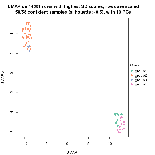
dimension_reduction(res, k = 2, method = "UMAP")

dimension_reduction(res, k = 3, method = "UMAP")

dimension_reduction(res, k = 4, method = "UMAP")
dimension_reduction(res, k = 5, method = "UMAP")
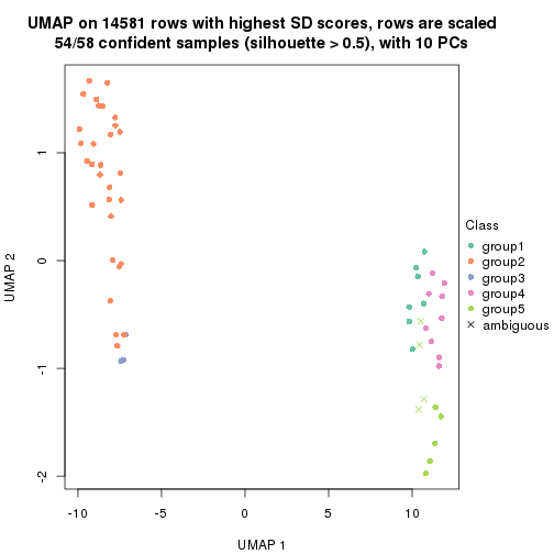
dimension_reduction(res, k = 6, method = "UMAP")

Following heatmap shows how subgroups are split when increasing k:
collect_classes(res)
If matrix rows can be associated to genes, consider to use functional_enrichment(res,
...) to perform function enrichment for the signature genes. See this vignette for more detailed explanations.
The object with results only for a single top-value method and a single partition method can be extracted as:
res = res_list["SD", "kmeans"]
# you can also extract it by
# res = res_list["SD:kmeans"]
A summary of res and all the functions that can be applied to it:
res
#> A 'ConsensusPartition' object with k = 2, 3, 4, 5, 6.
#>   On a matrix with 14581 rows and 58 columns.
#>   Top rows (1000, 2000, 3000, 4000, 5000) are extracted by 'SD' method.
#>   Subgroups are detected by 'kmeans' method.
#>   Performed in total 1250 partitions by row resampling.
#>   Best k for subgroups seems to be 2.
#>
#> Following methods can be applied to this 'ConsensusPartition' object:
#>  [1] "cola_report"             "collect_classes"         "collect_plots"
#>  [4] "collect_stats"           "colnames"                "compare_signatures"
#>  [7] "consensus_heatmap"       "dimension_reduction"     "functional_enrichment"
#> [10] "get_anno_col"            "get_anno"                "get_classes"
#> [13] "get_consensus"           "get_matrix"              "get_membership"
#> [16] "get_param"               "get_signatures"          "get_stats"
#> [19] "is_best_k"               "is_stable_k"             "membership_heatmap"
#> [22] "ncol"                    "nrow"                    "plot_ecdf"
#> [25] "rownames"                "select_partition_number" "show"
#> [28] "suggest_best_k"          "test_to_known_factors"
collect_plots() function collects all the plots made from res for all k (number of partitions)
into one single page to provide an easy and fast comparison between different k.
collect_plots(res)
The plots are:
k and the heatmap of
predicted classes for each k.k.k.k.All the plots in panels can be made by individual functions and they are plotted later in this section.
select_partition_number() produces several plots showing different
statistics for choosing “optimized” k. There are following statistics:
k;k, the area increased is defined as \(A_k - A_{k-1}\).The detailed explanations of these statistics can be found in the cola vignette.
Generally speaking, lower PAC score, higher mean silhouette score or higher
concordance corresponds to better partition. Rand index and Jaccard index
measure how similar the current partition is compared to partition with k-1.
If they are too similar, we won't accept k is better than k-1.
select_partition_number(res)
The numeric values for all these statistics can be obtained by get_stats().
get_stats(res)
#>   k 1-PAC mean_silhouette concordance area_increased  Rand Jaccard
#> 2 2 1.000           1.000       1.000         0.4996 0.501   0.501
#> 3 3 0.731           0.867       0.825         0.2428 0.861   0.722
#> 4 4 0.553           0.613       0.680         0.1091 0.918   0.773
#> 5 5 0.587           0.627       0.705         0.0927 0.913   0.730
#> 6 6 0.631           0.452       0.656         0.0513 0.976   0.917
suggest_best_k() suggests the best \(k\) based on these statistics. The rules are as follows:
suggest_best_k(res)
#> [1] 2
Following shows the table of the partitions (You need to click the show/hide
code output link to see it). The membership matrix (columns with name p*)
is inferred by
clue::cl_consensus()
function with the SE method. Basically the value in the membership matrix
represents the probability to belong to a certain group. The finall class
label for an item is determined with the group with highest probability it
belongs to.
In get_classes() function, the entropy is calculated from the membership
matrix and the silhouette score is calculated from the consensus matrix.
cbind(get_classes(res, k = 2), get_membership(res, k = 2))
#>           class entropy silhouette p1 p2
#> ERR789082     2       0          1  0  1
#> ERR789083     2       0          1  0  1
#> ERR789191     2       0          1  0  1
#> ERR789192     2       0          1  0  1
#> ERR789213     1       0          1  1  0
#> ERR789385     1       0          1  1  0
#> ERR789393     1       0          1  1  0
#> ERR789394     1       0          1  1  0
#> ERR789193     2       0          1  0  1
#> ERR789194     2       0          1  0  1
#> ERR789195     2       0          1  0  1
#> ERR789196     2       0          1  0  1
#> ERR789388     1       0          1  1  0
#> ERR789197     2       0          1  0  1
#> ERR789198     2       0          1  0  1
#> ERR789214     1       0          1  1  0
#> ERR789397     1       0          1  1  0
#> ERR789398     1       0          1  1  0
#> ERR789199     2       0          1  0  1
#> ERR789200     2       0          1  0  1
#> ERR789201     2       0          1  0  1
#> ERR789202     2       0          1  0  1
#> ERR789215     1       0          1  1  0
#> ERR789203     2       0          1  0  1
#> ERR789204     2       0          1  0  1
#> ERR789383     1       0          1  1  0
#> ERR789205     2       0          1  0  1
#> ERR789206     2       0          1  0  1
#> ERR789399     1       0          1  1  0
#> ERR789400     1       0          1  1  0
#> ERR789207     2       0          1  0  1
#> ERR789208     2       0          1  0  1
#> ERR789209     2       0          1  0  1
#> ERR789210     2       0          1  0  1
#> ERR789211     2       0          1  0  1
#> ERR789212     2       0          1  0  1
#> ERR789386     1       0          1  1  0
#> ERR789076     2       0          1  0  1
#> ERR789077     2       0          1  0  1
#> ERR789384     1       0          1  1  0
#> ERR789078     2       0          1  0  1
#> ERR789079     2       0          1  0  1
#> ERR789216     1       0          1  1  0
#> ERR789080     2       0          1  0  1
#> ERR789387     1       0          1  1  0
#> ERR789081     2       0          1  0  1
#> ERR789064     2       0          1  0  1
#> ERR779485     2       0          1  0  1
#> ERR789065     2       0          1  0  1
#> ERR789401     1       0          1  1  0
#> ERR789402     1       0          1  1  0
#> ERR789403     1       0          1  1  0
#> ERR789389     1       0          1  1  0
#> ERR789395     1       0          1  1  0
#> ERR789396     1       0          1  1  0
#> ERR789390     1       0          1  1  0
#> ERR789391     1       0          1  1  0
#> ERR789392     1       0          1  1  0
cbind(get_classes(res, k = 3), get_membership(res, k = 3))
#>           class entropy silhouette    p1    p2    p3
#> ERR789082     2  0.0747      0.929 0.000 0.984 0.016
#> ERR789083     2  0.0747      0.929 0.000 0.984 0.016
#> ERR789191     2  0.0747      0.929 0.000 0.984 0.016
#> ERR789192     2  0.0747      0.929 0.000 0.984 0.016
#> ERR789213     1  0.2959      0.872 0.900 0.000 0.100
#> ERR789385     1  0.2959      0.872 0.900 0.000 0.100
#> ERR789393     1  0.2448      0.876 0.924 0.000 0.076
#> ERR789394     1  0.2448      0.876 0.924 0.000 0.076
#> ERR789193     3  0.6008      0.915 0.000 0.372 0.628
#> ERR789194     3  0.6008      0.915 0.000 0.372 0.628
#> ERR789195     3  0.6252      0.932 0.000 0.444 0.556
#> ERR789196     3  0.6252      0.932 0.000 0.444 0.556
#> ERR789388     1  0.1289      0.882 0.968 0.000 0.032
#> ERR789197     2  0.0424      0.926 0.000 0.992 0.008
#> ERR789198     2  0.0424      0.926 0.000 0.992 0.008
#> ERR789214     1  0.3116      0.870 0.892 0.000 0.108
#> ERR789397     1  0.0892      0.883 0.980 0.000 0.020
#> ERR789398     1  0.0892      0.883 0.980 0.000 0.020
#> ERR789199     2  0.0592      0.926 0.000 0.988 0.012
#> ERR789200     2  0.0592      0.926 0.000 0.988 0.012
#> ERR789201     2  0.3551      0.699 0.000 0.868 0.132
#> ERR789202     2  0.3551      0.699 0.000 0.868 0.132
#> ERR789215     1  0.3941      0.881 0.844 0.000 0.156
#> ERR789203     3  0.6252      0.938 0.000 0.444 0.556
#> ERR789204     3  0.6252      0.938 0.000 0.444 0.556
#> ERR789383     1  0.5138      0.846 0.748 0.000 0.252
#> ERR789205     3  0.6252      0.938 0.000 0.444 0.556
#> ERR789206     3  0.6252      0.938 0.000 0.444 0.556
#> ERR789399     1  0.4702      0.860 0.788 0.000 0.212
#> ERR789400     1  0.4702      0.860 0.788 0.000 0.212
#> ERR789207     2  0.0592      0.931 0.000 0.988 0.012
#> ERR789208     2  0.0592      0.931 0.000 0.988 0.012
#> ERR789209     2  0.0592      0.931 0.000 0.988 0.012
#> ERR789210     2  0.0592      0.931 0.000 0.988 0.012
#> ERR789211     2  0.0592      0.931 0.000 0.988 0.012
#> ERR789212     2  0.0592      0.931 0.000 0.988 0.012
#> ERR789386     1  0.2959      0.872 0.900 0.000 0.100
#> ERR789076     2  0.6225     -0.639 0.000 0.568 0.432
#> ERR789077     2  0.0424      0.930 0.000 0.992 0.008
#> ERR789384     1  0.2959      0.872 0.900 0.000 0.100
#> ERR789078     2  0.0424      0.930 0.000 0.992 0.008
#> ERR789079     2  0.0424      0.930 0.000 0.992 0.008
#> ERR789216     1  0.2959      0.872 0.900 0.000 0.100
#> ERR789080     2  0.0424      0.930 0.000 0.992 0.008
#> ERR789387     1  0.2959      0.872 0.900 0.000 0.100
#> ERR789081     2  0.0424      0.930 0.000 0.992 0.008
#> ERR789064     2  0.0237      0.929 0.000 0.996 0.004
#> ERR779485     3  0.6026      0.919 0.000 0.376 0.624
#> ERR789065     3  0.6026      0.919 0.000 0.376 0.624
#> ERR789401     1  0.5138      0.846 0.748 0.000 0.252
#> ERR789402     1  0.5138      0.846 0.748 0.000 0.252
#> ERR789403     1  0.5138      0.846 0.748 0.000 0.252
#> ERR789389     1  0.5138      0.859 0.748 0.000 0.252
#> ERR789395     1  0.5138      0.846 0.748 0.000 0.252
#> ERR789396     1  0.5138      0.846 0.748 0.000 0.252
#> ERR789390     1  0.3619      0.876 0.864 0.000 0.136
#> ERR789391     1  0.3619      0.876 0.864 0.000 0.136
#> ERR789392     1  0.2448      0.876 0.924 0.000 0.076
cbind(get_classes(res, k = 4), get_membership(res, k = 4))
#>           class entropy silhouette    p1    p2    p3    p4
#> ERR789082     2  0.1940     0.8383 0.000 0.924 0.000 0.076
#> ERR789083     2  0.1940     0.8383 0.000 0.924 0.000 0.076
#> ERR789191     2  0.2469     0.8340 0.000 0.892 0.000 0.108
#> ERR789192     2  0.2469     0.8340 0.000 0.892 0.000 0.108
#> ERR789213     4  0.6315     0.8079 0.396 0.000 0.064 0.540
#> ERR789385     4  0.6315     0.8079 0.396 0.000 0.064 0.540
#> ERR789393     1  0.6709    -0.6530 0.456 0.000 0.088 0.456
#> ERR789394     1  0.6709    -0.6530 0.456 0.000 0.088 0.456
#> ERR789193     3  0.6374     0.8098 0.000 0.228 0.644 0.128
#> ERR789194     3  0.6374     0.8098 0.000 0.228 0.644 0.128
#> ERR789195     3  0.6005     0.8068 0.000 0.324 0.616 0.060
#> ERR789196     3  0.6005     0.8068 0.000 0.324 0.616 0.060
#> ERR789388     4  0.6148     0.6406 0.468 0.000 0.048 0.484
#> ERR789197     2  0.4037     0.7769 0.000 0.832 0.056 0.112
#> ERR789198     2  0.4037     0.7769 0.000 0.832 0.056 0.112
#> ERR789214     4  0.5980     0.8272 0.396 0.000 0.044 0.560
#> ERR789397     1  0.6383    -0.2985 0.568 0.000 0.076 0.356
#> ERR789398     1  0.6383    -0.2985 0.568 0.000 0.076 0.356
#> ERR789199     2  0.3464     0.8008 0.000 0.860 0.032 0.108
#> ERR789200     2  0.3464     0.8008 0.000 0.860 0.032 0.108
#> ERR789201     2  0.5035     0.5921 0.000 0.748 0.196 0.056
#> ERR789202     2  0.5035     0.5921 0.000 0.748 0.196 0.056
#> ERR789215     1  0.6516    -0.0884 0.592 0.000 0.100 0.308
#> ERR789203     3  0.5130     0.8501 0.000 0.312 0.668 0.020
#> ERR789204     3  0.5130     0.8501 0.000 0.312 0.668 0.020
#> ERR789383     1  0.1807     0.5756 0.940 0.000 0.052 0.008
#> ERR789205     3  0.5453     0.8408 0.000 0.320 0.648 0.032
#> ERR789206     3  0.5453     0.8408 0.000 0.320 0.648 0.032
#> ERR789399     1  0.3037     0.5710 0.888 0.000 0.076 0.036
#> ERR789400     1  0.3037     0.5710 0.888 0.000 0.076 0.036
#> ERR789207     2  0.1890     0.8377 0.000 0.936 0.008 0.056
#> ERR789208     2  0.1890     0.8377 0.000 0.936 0.008 0.056
#> ERR789209     2  0.2589     0.8171 0.000 0.912 0.044 0.044
#> ERR789210     2  0.2589     0.8171 0.000 0.912 0.044 0.044
#> ERR789211     2  0.1767     0.8324 0.000 0.944 0.012 0.044
#> ERR789212     2  0.1767     0.8324 0.000 0.944 0.012 0.044
#> ERR789386     4  0.5766     0.8662 0.404 0.000 0.032 0.564
#> ERR789076     2  0.6690    -0.1607 0.000 0.548 0.352 0.100
#> ERR789077     2  0.2704     0.8153 0.000 0.876 0.000 0.124
#> ERR789384     4  0.5487     0.8675 0.400 0.000 0.020 0.580
#> ERR789078     2  0.2704     0.8153 0.000 0.876 0.000 0.124
#> ERR789079     2  0.2530     0.8170 0.000 0.888 0.000 0.112
#> ERR789216     4  0.5766     0.8662 0.404 0.000 0.032 0.564
#> ERR789080     2  0.2530     0.8170 0.000 0.888 0.000 0.112
#> ERR789387     4  0.5999     0.8495 0.404 0.000 0.044 0.552
#> ERR789081     2  0.2530     0.8170 0.000 0.888 0.000 0.112
#> ERR789064     2  0.0817     0.8438 0.000 0.976 0.000 0.024
#> ERR779485     3  0.6327     0.8098 0.000 0.228 0.648 0.124
#> ERR789065     3  0.5008     0.8330 0.000 0.228 0.732 0.040
#> ERR789401     1  0.0336     0.5919 0.992 0.000 0.008 0.000
#> ERR789402     1  0.0469     0.5917 0.988 0.000 0.012 0.000
#> ERR789403     1  0.0336     0.5919 0.992 0.000 0.008 0.000
#> ERR789389     1  0.4462     0.3993 0.792 0.000 0.044 0.164
#> ERR789395     1  0.0469     0.5917 0.988 0.000 0.012 0.000
#> ERR789396     1  0.0469     0.5917 0.988 0.000 0.012 0.000
#> ERR789390     1  0.4663     0.4529 0.788 0.000 0.064 0.148
#> ERR789391     1  0.4663     0.4529 0.788 0.000 0.064 0.148
#> ERR789392     1  0.6709    -0.6530 0.456 0.000 0.088 0.456
cbind(get_classes(res, k = 5), get_membership(res, k = 5))
#>           class entropy silhouette    p1    p2    p3    p4 p5
#> ERR789082     2  0.3012      0.731 0.024 0.852 0.000 0.000 NA
#> ERR789083     2  0.3012      0.731 0.024 0.852 0.000 0.000 NA
#> ERR789191     2  0.3090      0.725 0.040 0.856 0.000 0.000 NA
#> ERR789192     2  0.3090      0.725 0.040 0.856 0.000 0.000 NA
#> ERR789213     4  0.2439      0.636 0.000 0.000 0.004 0.876 NA
#> ERR789385     4  0.2439      0.636 0.000 0.000 0.004 0.876 NA
#> ERR789393     4  0.4766      0.577 0.072 0.000 0.000 0.708 NA
#> ERR789394     4  0.4766      0.577 0.072 0.000 0.000 0.708 NA
#> ERR789193     3  0.5904      0.770 0.148 0.080 0.688 0.000 NA
#> ERR789194     3  0.5904      0.770 0.148 0.080 0.688 0.000 NA
#> ERR789195     3  0.5999      0.696 0.016 0.112 0.608 0.000 NA
#> ERR789196     3  0.5999      0.696 0.016 0.112 0.608 0.000 NA
#> ERR789388     4  0.4302      0.583 0.088 0.000 0.044 0.808 NA
#> ERR789197     2  0.5176      0.575 0.004 0.560 0.036 0.000 NA
#> ERR789198     2  0.5176      0.575 0.004 0.560 0.036 0.000 NA
#> ERR789214     4  0.2291      0.640 0.012 0.000 0.024 0.916 NA
#> ERR789397     4  0.6437      0.427 0.192 0.000 0.040 0.612 NA
#> ERR789398     4  0.6437      0.427 0.192 0.000 0.040 0.612 NA
#> ERR789199     2  0.4879      0.630 0.020 0.636 0.012 0.000 NA
#> ERR789200     2  0.4879      0.630 0.020 0.636 0.012 0.000 NA
#> ERR789201     2  0.6708      0.271 0.012 0.464 0.352 0.000 NA
#> ERR789202     2  0.6708      0.271 0.012 0.464 0.352 0.000 NA
#> ERR789215     4  0.5094      0.380 0.176 0.000 0.020 0.724 NA
#> ERR789203     3  0.3533      0.801 0.004 0.104 0.836 0.000 NA
#> ERR789204     3  0.3533      0.801 0.004 0.104 0.836 0.000 NA
#> ERR789383     1  0.5208      0.852 0.624 0.000 0.020 0.328 NA
#> ERR789205     3  0.4350      0.781 0.008 0.108 0.784 0.000 NA
#> ERR789206     3  0.4350      0.781 0.008 0.108 0.784 0.000 NA
#> ERR789399     1  0.6235      0.751 0.540 0.000 0.024 0.348 NA
#> ERR789400     1  0.6235      0.751 0.540 0.000 0.024 0.348 NA
#> ERR789207     2  0.3155      0.724 0.008 0.848 0.016 0.000 NA
#> ERR789208     2  0.3155      0.724 0.008 0.848 0.016 0.000 NA
#> ERR789209     2  0.4883      0.685 0.012 0.732 0.076 0.000 NA
#> ERR789210     2  0.4883      0.685 0.012 0.732 0.076 0.000 NA
#> ERR789211     2  0.4379      0.703 0.012 0.764 0.044 0.000 NA
#> ERR789212     2  0.4379      0.703 0.012 0.764 0.044 0.000 NA
#> ERR789386     4  0.0955      0.640 0.004 0.000 0.000 0.968 NA
#> ERR789076     2  0.7326      0.151 0.060 0.472 0.308 0.000 NA
#> ERR789077     2  0.3759      0.709 0.092 0.816 0.000 0.000 NA
#> ERR789384     4  0.0510      0.645 0.000 0.000 0.000 0.984 NA
#> ERR789078     2  0.3759      0.709 0.092 0.816 0.000 0.000 NA
#> ERR789079     2  0.3593      0.713 0.088 0.828 0.000 0.000 NA
#> ERR789216     4  0.0955      0.640 0.004 0.000 0.000 0.968 NA
#> ERR789080     2  0.3593      0.713 0.088 0.828 0.000 0.000 NA
#> ERR789387     4  0.1041      0.638 0.004 0.000 0.000 0.964 NA
#> ERR789081     2  0.3593      0.713 0.088 0.828 0.000 0.000 NA
#> ERR789064     2  0.3053      0.741 0.008 0.852 0.012 0.000 NA
#> ERR779485     3  0.5850      0.771 0.148 0.076 0.692 0.000 NA
#> ERR789065     3  0.4007      0.802 0.084 0.076 0.820 0.000 NA
#> ERR789401     1  0.3837      0.900 0.692 0.000 0.000 0.308 NA
#> ERR789402     1  0.4385      0.900 0.672 0.000 0.012 0.312 NA
#> ERR789403     1  0.3837      0.900 0.692 0.000 0.000 0.308 NA
#> ERR789389     4  0.5426     -0.337 0.408 0.000 0.016 0.544 NA
#> ERR789395     1  0.4385      0.900 0.672 0.000 0.012 0.312 NA
#> ERR789396     1  0.4385      0.900 0.672 0.000 0.012 0.312 NA
#> ERR789390     4  0.6870     -0.204 0.368 0.000 0.032 0.464 NA
#> ERR789391     4  0.6870     -0.204 0.368 0.000 0.032 0.464 NA
#> ERR789392     4  0.4766      0.577 0.072 0.000 0.000 0.708 NA
cbind(get_classes(res, k = 6), get_membership(res, k = 6))
#>           class entropy silhouette    p1    p2    p3    p4    p5 p6
#> ERR789082     2  0.1624    0.67058 0.008 0.936 0.000 0.000 0.012 NA
#> ERR789083     2  0.1624    0.67058 0.008 0.936 0.000 0.000 0.012 NA
#> ERR789191     2  0.0881    0.66568 0.008 0.972 0.000 0.000 0.008 NA
#> ERR789192     2  0.0881    0.66568 0.008 0.972 0.000 0.000 0.008 NA
#> ERR789213     4  0.2613    0.28881 0.000 0.000 0.012 0.848 0.140 NA
#> ERR789385     4  0.2613    0.28881 0.000 0.000 0.012 0.848 0.140 NA
#> ERR789393     4  0.1219    0.34883 0.048 0.000 0.000 0.948 0.000 NA
#> ERR789394     4  0.1219    0.34883 0.048 0.000 0.000 0.948 0.000 NA
#> ERR789193     3  0.1226    0.69774 0.000 0.040 0.952 0.000 0.004 NA
#> ERR789194     3  0.1226    0.69774 0.000 0.040 0.952 0.000 0.004 NA
#> ERR789195     3  0.7622    0.63597 0.032 0.092 0.420 0.000 0.204 NA
#> ERR789196     3  0.7622    0.63597 0.032 0.092 0.420 0.000 0.204 NA
#> ERR789388     4  0.6622   -0.05994 0.068 0.000 0.024 0.500 0.328 NA
#> ERR789197     2  0.5951    0.50467 0.048 0.580 0.000 0.000 0.124 NA
#> ERR789198     2  0.5951    0.50467 0.048 0.580 0.000 0.000 0.124 NA
#> ERR789214     4  0.5515    0.08170 0.004 0.000 0.024 0.556 0.348 NA
#> ERR789397     4  0.6415    0.16670 0.184 0.000 0.020 0.600 0.112 NA
#> ERR789398     4  0.6415    0.16670 0.184 0.000 0.020 0.600 0.112 NA
#> ERR789199     2  0.5413    0.56579 0.040 0.652 0.000 0.000 0.108 NA
#> ERR789200     2  0.5413    0.56579 0.040 0.652 0.000 0.000 0.108 NA
#> ERR789201     2  0.7372    0.07857 0.000 0.336 0.112 0.000 0.256 NA
#> ERR789202     2  0.7372    0.07857 0.000 0.336 0.112 0.000 0.256 NA
#> ERR789215     5  0.7245    0.00000 0.176 0.000 0.004 0.344 0.372 NA
#> ERR789203     3  0.6338    0.76070 0.000 0.064 0.536 0.000 0.260 NA
#> ERR789204     3  0.6338    0.76070 0.000 0.064 0.536 0.000 0.260 NA
#> ERR789383     1  0.5678    0.66479 0.652 0.000 0.004 0.180 0.068 NA
#> ERR789205     3  0.6558    0.74967 0.000 0.064 0.500 0.000 0.268 NA
#> ERR789206     3  0.6558    0.74967 0.000 0.064 0.500 0.000 0.268 NA
#> ERR789399     1  0.6225    0.57032 0.556 0.000 0.000 0.252 0.068 NA
#> ERR789400     1  0.6225    0.57032 0.556 0.000 0.000 0.252 0.068 NA
#> ERR789207     2  0.3795    0.65394 0.000 0.632 0.000 0.000 0.004 NA
#> ERR789208     2  0.3795    0.65394 0.000 0.632 0.000 0.000 0.004 NA
#> ERR789209     2  0.4093    0.60864 0.000 0.516 0.000 0.000 0.008 NA
#> ERR789210     2  0.4093    0.60864 0.000 0.516 0.000 0.000 0.008 NA
#> ERR789211     2  0.3838    0.63216 0.000 0.552 0.000 0.000 0.000 NA
#> ERR789212     2  0.3838    0.63216 0.000 0.552 0.000 0.000 0.000 NA
#> ERR789386     4  0.3955   -0.02028 0.004 0.000 0.000 0.560 0.436 NA
#> ERR789076     2  0.8155    0.11109 0.076 0.328 0.192 0.000 0.092 NA
#> ERR789077     2  0.4984    0.62867 0.072 0.704 0.000 0.000 0.052 NA
#> ERR789384     4  0.4063    0.00876 0.004 0.000 0.004 0.572 0.420 NA
#> ERR789078     2  0.4984    0.62867 0.072 0.704 0.000 0.000 0.052 NA
#> ERR789079     2  0.5033    0.63684 0.060 0.672 0.000 0.000 0.040 NA
#> ERR789216     4  0.3955   -0.02028 0.004 0.000 0.000 0.560 0.436 NA
#> ERR789080     2  0.5033    0.63684 0.060 0.672 0.000 0.000 0.040 NA
#> ERR789387     4  0.4208   -0.11364 0.008 0.000 0.000 0.536 0.452 NA
#> ERR789081     2  0.5033    0.63684 0.060 0.672 0.000 0.000 0.040 NA
#> ERR789064     2  0.3197    0.68081 0.012 0.804 0.000 0.000 0.008 NA
#> ERR779485     3  0.1965    0.69720 0.024 0.040 0.924 0.000 0.008 NA
#> ERR789065     3  0.4817    0.74965 0.028 0.040 0.748 0.000 0.136 NA
#> ERR789401     1  0.3231    0.75919 0.800 0.000 0.000 0.180 0.008 NA
#> ERR789402     1  0.3502    0.75810 0.788 0.000 0.004 0.184 0.012 NA
#> ERR789403     1  0.3231    0.75919 0.800 0.000 0.000 0.180 0.008 NA
#> ERR789389     1  0.6635   -0.50370 0.368 0.000 0.004 0.272 0.336 NA
#> ERR789395     1  0.3502    0.75810 0.788 0.000 0.004 0.184 0.012 NA
#> ERR789396     1  0.3502    0.75810 0.788 0.000 0.004 0.184 0.012 NA
#> ERR789390     4  0.6220   -0.29076 0.424 0.000 0.008 0.440 0.056 NA
#> ERR789391     4  0.6220   -0.29076 0.424 0.000 0.008 0.440 0.056 NA
#> ERR789392     4  0.1219    0.34883 0.048 0.000 0.000 0.948 0.000 NA
Heatmaps for the consensus matrix. It visualizes the probability of two samples to be in a same group.
consensus_heatmap(res, k = 2)

consensus_heatmap(res, k = 3)
consensus_heatmap(res, k = 4)
consensus_heatmap(res, k = 5)
consensus_heatmap(res, k = 6)
Heatmaps for the membership of samples in all partitions to see how consistent they are:
membership_heatmap(res, k = 2)

membership_heatmap(res, k = 3)
membership_heatmap(res, k = 4)
membership_heatmap(res, k = 5)
membership_heatmap(res, k = 6)

As soon as we have had the classes for columns, we can look for signatures which are significantly different between classes which can be candidate marks for certain classes. Following are the heatmaps for signatures.
Signature heatmaps where rows are scaled:
get_signatures(res, k = 2)

get_signatures(res, k = 3)
get_signatures(res, k = 4)
get_signatures(res, k = 5)
get_signatures(res, k = 6)
Signature heatmaps where rows are not scaled:
get_signatures(res, k = 2, scale_rows = FALSE)

get_signatures(res, k = 3, scale_rows = FALSE)
get_signatures(res, k = 4, scale_rows = FALSE)
get_signatures(res, k = 5, scale_rows = FALSE)
get_signatures(res, k = 6, scale_rows = FALSE)
Compare the overlap of signatures from different k:
compare_signatures(res)
get_signature() returns a data frame invisibly. TO get the list of signatures, the function
call should be assigned to a variable explicitly. In following code, if plot argument is set
to FALSE, no heatmap is plotted while only the differential analysis is performed.
# code only for demonstration
tb = get_signature(res, k = ..., plot = FALSE)
An example of the output of tb is:
#>   which_row         fdr    mean_1    mean_2 scaled_mean_1 scaled_mean_2 km
#> 1        38 0.042760348  8.373488  9.131774    -0.5533452     0.5164555  1
#> 2        40 0.018707592  7.106213  8.469186    -0.6173731     0.5762149  1
#> 3        55 0.019134737 10.221463 11.207825    -0.6159697     0.5749050  1
#> 4        59 0.006059896  5.921854  7.869574    -0.6899429     0.6439467  1
#> 5        60 0.018055526  8.928898 10.211722    -0.6204761     0.5791110  1
#> 6        98 0.009384629 15.714769 14.887706     0.6635654    -0.6193277  2
...
The columns in tb are:
which_row: row indices corresponding to the input matrix.fdr: FDR for the differential test. mean_x: The mean value in group x.scaled_mean_x: The mean value in group x after rows are scaled.km: Row groups if k-means clustering is applied to rows.UMAP plot which shows how samples are separated.
dimension_reduction(res, k = 2, method = "UMAP")

dimension_reduction(res, k = 3, method = "UMAP")

dimension_reduction(res, k = 4, method = "UMAP")

dimension_reduction(res, k = 5, method = "UMAP")
dimension_reduction(res, k = 6, method = "UMAP")
Following heatmap shows how subgroups are split when increasing k:
collect_classes(res)
If matrix rows can be associated to genes, consider to use functional_enrichment(res,
...) to perform function enrichment for the signature genes. See this vignette for more detailed explanations.
The object with results only for a single top-value method and a single partition method can be extracted as:
res = res_list["SD", "skmeans"]
# you can also extract it by
# res = res_list["SD:skmeans"]
A summary of res and all the functions that can be applied to it:
res
#> A 'ConsensusPartition' object with k = 2, 3, 4, 5, 6.
#>   On a matrix with 14581 rows and 58 columns.
#>   Top rows (1000, 2000, 3000, 4000, 5000) are extracted by 'SD' method.
#>   Subgroups are detected by 'skmeans' method.
#>   Performed in total 1250 partitions by row resampling.
#>   Best k for subgroups seems to be 2.
#>
#> Following methods can be applied to this 'ConsensusPartition' object:
#>  [1] "cola_report"             "collect_classes"         "collect_plots"
#>  [4] "collect_stats"           "colnames"                "compare_signatures"
#>  [7] "consensus_heatmap"       "dimension_reduction"     "functional_enrichment"
#> [10] "get_anno_col"            "get_anno"                "get_classes"
#> [13] "get_consensus"           "get_matrix"              "get_membership"
#> [16] "get_param"               "get_signatures"          "get_stats"
#> [19] "is_best_k"               "is_stable_k"             "membership_heatmap"
#> [22] "ncol"                    "nrow"                    "plot_ecdf"
#> [25] "rownames"                "select_partition_number" "show"
#> [28] "suggest_best_k"          "test_to_known_factors"
collect_plots() function collects all the plots made from res for all k (number of partitions)
into one single page to provide an easy and fast comparison between different k.
collect_plots(res)
The plots are:
k and the heatmap of
predicted classes for each k.k.k.k.All the plots in panels can be made by individual functions and they are plotted later in this section.
select_partition_number() produces several plots showing different
statistics for choosing “optimized” k. There are following statistics:
k;k, the area increased is defined as \(A_k - A_{k-1}\).The detailed explanations of these statistics can be found in the cola vignette.
Generally speaking, lower PAC score, higher mean silhouette score or higher
concordance corresponds to better partition. Rand index and Jaccard index
measure how similar the current partition is compared to partition with k-1.
If they are too similar, we won't accept k is better than k-1.
select_partition_number(res)
The numeric values for all these statistics can be obtained by get_stats().
get_stats(res)
#>   k 1-PAC mean_silhouette concordance area_increased  Rand Jaccard
#> 2 2 1.000           1.000       1.000         0.4996 0.501   0.501
#> 3 3 0.888           0.941       0.949         0.2231 0.861   0.722
#> 4 4 0.741           0.543       0.818         0.1384 0.972   0.923
#> 5 5 0.656           0.680       0.806         0.0758 0.863   0.613
#> 6 6 0.675           0.620       0.742         0.0513 0.985   0.941
suggest_best_k() suggests the best \(k\) based on these statistics. The rules are as follows:
suggest_best_k(res)
#> [1] 2
Following shows the table of the partitions (You need to click the show/hide
code output link to see it). The membership matrix (columns with name p*)
is inferred by
clue::cl_consensus()
function with the SE method. Basically the value in the membership matrix
represents the probability to belong to a certain group. The finall class
label for an item is determined with the group with highest probability it
belongs to.
In get_classes() function, the entropy is calculated from the membership
matrix and the silhouette score is calculated from the consensus matrix.
cbind(get_classes(res, k = 2), get_membership(res, k = 2))
#>           class entropy silhouette p1 p2
#> ERR789082     2       0          1  0  1
#> ERR789083     2       0          1  0  1
#> ERR789191     2       0          1  0  1
#> ERR789192     2       0          1  0  1
#> ERR789213     1       0          1  1  0
#> ERR789385     1       0          1  1  0
#> ERR789393     1       0          1  1  0
#> ERR789394     1       0          1  1  0
#> ERR789193     2       0          1  0  1
#> ERR789194     2       0          1  0  1
#> ERR789195     2       0          1  0  1
#> ERR789196     2       0          1  0  1
#> ERR789388     1       0          1  1  0
#> ERR789197     2       0          1  0  1
#> ERR789198     2       0          1  0  1
#> ERR789214     1       0          1  1  0
#> ERR789397     1       0          1  1  0
#> ERR789398     1       0          1  1  0
#> ERR789199     2       0          1  0  1
#> ERR789200     2       0          1  0  1
#> ERR789201     2       0          1  0  1
#> ERR789202     2       0          1  0  1
#> ERR789215     1       0          1  1  0
#> ERR789203     2       0          1  0  1
#> ERR789204     2       0          1  0  1
#> ERR789383     1       0          1  1  0
#> ERR789205     2       0          1  0  1
#> ERR789206     2       0          1  0  1
#> ERR789399     1       0          1  1  0
#> ERR789400     1       0          1  1  0
#> ERR789207     2       0          1  0  1
#> ERR789208     2       0          1  0  1
#> ERR789209     2       0          1  0  1
#> ERR789210     2       0          1  0  1
#> ERR789211     2       0          1  0  1
#> ERR789212     2       0          1  0  1
#> ERR789386     1       0          1  1  0
#> ERR789076     2       0          1  0  1
#> ERR789077     2       0          1  0  1
#> ERR789384     1       0          1  1  0
#> ERR789078     2       0          1  0  1
#> ERR789079     2       0          1  0  1
#> ERR789216     1       0          1  1  0
#> ERR789080     2       0          1  0  1
#> ERR789387     1       0          1  1  0
#> ERR789081     2       0          1  0  1
#> ERR789064     2       0          1  0  1
#> ERR779485     2       0          1  0  1
#> ERR789065     2       0          1  0  1
#> ERR789401     1       0          1  1  0
#> ERR789402     1       0          1  1  0
#> ERR789403     1       0          1  1  0
#> ERR789389     1       0          1  1  0
#> ERR789395     1       0          1  1  0
#> ERR789396     1       0          1  1  0
#> ERR789390     1       0          1  1  0
#> ERR789391     1       0          1  1  0
#> ERR789392     1       0          1  1  0
cbind(get_classes(res, k = 3), get_membership(res, k = 3))
#>           class entropy silhouette p1    p2    p3
#> ERR789082     2  0.0000      0.976  0 1.000 0.000
#> ERR789083     2  0.0000      0.976  0 1.000 0.000
#> ERR789191     2  0.0000      0.976  0 1.000 0.000
#> ERR789192     2  0.0000      0.976  0 1.000 0.000
#> ERR789213     1  0.0000      1.000  1 0.000 0.000
#> ERR789385     1  0.0000      1.000  1 0.000 0.000
#> ERR789393     1  0.0000      1.000  1 0.000 0.000
#> ERR789394     1  0.0000      1.000  1 0.000 0.000
#> ERR789193     3  0.1753      0.677  0 0.048 0.952
#> ERR789194     3  0.1753      0.677  0 0.048 0.952
#> ERR789195     3  0.6026      0.761  0 0.376 0.624
#> ERR789196     3  0.6026      0.761  0 0.376 0.624
#> ERR789388     1  0.0000      1.000  1 0.000 0.000
#> ERR789197     2  0.1643      0.949  0 0.956 0.044
#> ERR789198     2  0.1643      0.949  0 0.956 0.044
#> ERR789214     1  0.0000      1.000  1 0.000 0.000
#> ERR789397     1  0.0000      1.000  1 0.000 0.000
#> ERR789398     1  0.0000      1.000  1 0.000 0.000
#> ERR789199     2  0.1643      0.949  0 0.956 0.044
#> ERR789200     2  0.1643      0.949  0 0.956 0.044
#> ERR789201     2  0.2356      0.922  0 0.928 0.072
#> ERR789202     2  0.2356      0.922  0 0.928 0.072
#> ERR789215     1  0.0000      1.000  1 0.000 0.000
#> ERR789203     3  0.5968      0.770  0 0.364 0.636
#> ERR789204     3  0.5968      0.770  0 0.364 0.636
#> ERR789383     1  0.0000      1.000  1 0.000 0.000
#> ERR789205     3  0.5988      0.768  0 0.368 0.632
#> ERR789206     3  0.5988      0.768  0 0.368 0.632
#> ERR789399     1  0.0000      1.000  1 0.000 0.000
#> ERR789400     1  0.0000      1.000  1 0.000 0.000
#> ERR789207     2  0.0237      0.975  0 0.996 0.004
#> ERR789208     2  0.0237      0.975  0 0.996 0.004
#> ERR789209     2  0.0237      0.975  0 0.996 0.004
#> ERR789210     2  0.0237      0.975  0 0.996 0.004
#> ERR789211     2  0.0237      0.975  0 0.996 0.004
#> ERR789212     2  0.0237      0.975  0 0.996 0.004
#> ERR789386     1  0.0000      1.000  1 0.000 0.000
#> ERR789076     2  0.0000      0.976  0 1.000 0.000
#> ERR789077     2  0.0000      0.976  0 1.000 0.000
#> ERR789384     1  0.0000      1.000  1 0.000 0.000
#> ERR789078     2  0.0000      0.976  0 1.000 0.000
#> ERR789079     2  0.0000      0.976  0 1.000 0.000
#> ERR789216     1  0.0000      1.000  1 0.000 0.000
#> ERR789080     2  0.0000      0.976  0 1.000 0.000
#> ERR789387     1  0.0000      1.000  1 0.000 0.000
#> ERR789081     2  0.0000      0.976  0 1.000 0.000
#> ERR789064     2  0.1753      0.947  0 0.952 0.048
#> ERR779485     3  0.0000      0.678  0 0.000 1.000
#> ERR789065     3  0.4931      0.755  0 0.232 0.768
#> ERR789401     1  0.0000      1.000  1 0.000 0.000
#> ERR789402     1  0.0000      1.000  1 0.000 0.000
#> ERR789403     1  0.0000      1.000  1 0.000 0.000
#> ERR789389     1  0.0000      1.000  1 0.000 0.000
#> ERR789395     1  0.0000      1.000  1 0.000 0.000
#> ERR789396     1  0.0000      1.000  1 0.000 0.000
#> ERR789390     1  0.0000      1.000  1 0.000 0.000
#> ERR789391     1  0.0000      1.000  1 0.000 0.000
#> ERR789392     1  0.0000      1.000  1 0.000 0.000
cbind(get_classes(res, k = 4), get_membership(res, k = 4))
#>           class entropy silhouette    p1    p2    p3    p4
#> ERR789082     2  0.0000      0.902 0.000 1.000 0.000 0.000
#> ERR789083     2  0.0000      0.902 0.000 1.000 0.000 0.000
#> ERR789191     2  0.0000      0.902 0.000 1.000 0.000 0.000
#> ERR789192     2  0.0000      0.902 0.000 1.000 0.000 0.000
#> ERR789213     4  0.4972      1.000 0.456 0.000 0.000 0.544
#> ERR789385     4  0.4972      1.000 0.456 0.000 0.000 0.544
#> ERR789393     1  0.4994     -0.788 0.520 0.000 0.000 0.480
#> ERR789394     1  0.4994     -0.788 0.520 0.000 0.000 0.480
#> ERR789193     3  0.5493      0.648 0.000 0.016 0.528 0.456
#> ERR789194     3  0.5493      0.648 0.000 0.016 0.528 0.456
#> ERR789195     3  0.3400      0.747 0.000 0.180 0.820 0.000
#> ERR789196     3  0.3400      0.747 0.000 0.180 0.820 0.000
#> ERR789388     1  0.3356      0.441 0.824 0.000 0.000 0.176
#> ERR789197     2  0.3975      0.737 0.000 0.760 0.240 0.000
#> ERR789198     2  0.3975      0.737 0.000 0.760 0.240 0.000
#> ERR789214     1  0.4948     -0.637 0.560 0.000 0.000 0.440
#> ERR789397     1  0.2704      0.492 0.876 0.000 0.000 0.124
#> ERR789398     1  0.2704      0.492 0.876 0.000 0.000 0.124
#> ERR789199     2  0.3444      0.796 0.000 0.816 0.184 0.000
#> ERR789200     2  0.3444      0.796 0.000 0.816 0.184 0.000
#> ERR789201     2  0.4907      0.446 0.000 0.580 0.420 0.000
#> ERR789202     2  0.4907      0.446 0.000 0.580 0.420 0.000
#> ERR789215     1  0.1716      0.571 0.936 0.000 0.000 0.064
#> ERR789203     3  0.1867      0.824 0.000 0.072 0.928 0.000
#> ERR789204     3  0.1867      0.824 0.000 0.072 0.928 0.000
#> ERR789383     1  0.1557      0.577 0.944 0.000 0.000 0.056
#> ERR789205     3  0.1867      0.824 0.000 0.072 0.928 0.000
#> ERR789206     3  0.1867      0.824 0.000 0.072 0.928 0.000
#> ERR789399     1  0.0000      0.611 1.000 0.000 0.000 0.000
#> ERR789400     1  0.0000      0.611 1.000 0.000 0.000 0.000
#> ERR789207     2  0.0592      0.901 0.000 0.984 0.016 0.000
#> ERR789208     2  0.0592      0.901 0.000 0.984 0.016 0.000
#> ERR789209     2  0.1557      0.892 0.000 0.944 0.056 0.000
#> ERR789210     2  0.1557      0.892 0.000 0.944 0.056 0.000
#> ERR789211     2  0.1118      0.898 0.000 0.964 0.036 0.000
#> ERR789212     2  0.1118      0.898 0.000 0.964 0.036 0.000
#> ERR789386     1  0.4985     -0.725 0.532 0.000 0.000 0.468
#> ERR789076     2  0.0707      0.899 0.000 0.980 0.020 0.000
#> ERR789077     2  0.0000      0.902 0.000 1.000 0.000 0.000
#> ERR789384     1  0.4989     -0.740 0.528 0.000 0.000 0.472
#> ERR789078     2  0.0000      0.902 0.000 1.000 0.000 0.000
#> ERR789079     2  0.0000      0.902 0.000 1.000 0.000 0.000
#> ERR789216     1  0.4985     -0.725 0.532 0.000 0.000 0.468
#> ERR789080     2  0.0000      0.902 0.000 1.000 0.000 0.000
#> ERR789387     1  0.4985     -0.725 0.532 0.000 0.000 0.468
#> ERR789081     2  0.0000      0.902 0.000 1.000 0.000 0.000
#> ERR789064     2  0.2149      0.868 0.000 0.912 0.088 0.000
#> ERR779485     3  0.4817      0.677 0.000 0.000 0.612 0.388
#> ERR789065     3  0.3247      0.816 0.000 0.060 0.880 0.060
#> ERR789401     1  0.0000      0.611 1.000 0.000 0.000 0.000
#> ERR789402     1  0.0000      0.611 1.000 0.000 0.000 0.000
#> ERR789403     1  0.0000      0.611 1.000 0.000 0.000 0.000
#> ERR789389     1  0.2149      0.557 0.912 0.000 0.000 0.088
#> ERR789395     1  0.0000      0.611 1.000 0.000 0.000 0.000
#> ERR789396     1  0.0000      0.611 1.000 0.000 0.000 0.000
#> ERR789390     1  0.0000      0.611 1.000 0.000 0.000 0.000
#> ERR789391     1  0.0000      0.611 1.000 0.000 0.000 0.000
#> ERR789392     1  0.4994     -0.788 0.520 0.000 0.000 0.480
cbind(get_classes(res, k = 5), get_membership(res, k = 5))
#>           class entropy silhouette    p1    p2    p3    p4    p5
#> ERR789082     2  0.0451    0.83244 0.004 0.988 0.008 0.000 0.000
#> ERR789083     2  0.0451    0.83244 0.004 0.988 0.008 0.000 0.000
#> ERR789191     2  0.0162    0.83151 0.004 0.996 0.000 0.000 0.000
#> ERR789192     2  0.0162    0.83151 0.004 0.996 0.000 0.000 0.000
#> ERR789213     4  0.1792    0.66520 0.000 0.000 0.000 0.916 0.084
#> ERR789385     4  0.1792    0.66520 0.000 0.000 0.000 0.916 0.084
#> ERR789393     4  0.4482    0.58080 0.160 0.000 0.000 0.752 0.088
#> ERR789394     4  0.4482    0.58080 0.160 0.000 0.000 0.752 0.088
#> ERR789193     5  0.1851    0.91594 0.000 0.000 0.088 0.000 0.912
#> ERR789194     5  0.1851    0.91594 0.000 0.000 0.088 0.000 0.912
#> ERR789195     3  0.4088    0.70162 0.064 0.140 0.792 0.000 0.004
#> ERR789196     3  0.4088    0.70162 0.064 0.140 0.792 0.000 0.004
#> ERR789388     4  0.4310   -0.00252 0.392 0.000 0.004 0.604 0.000
#> ERR789197     2  0.5498    0.14220 0.064 0.496 0.440 0.000 0.000
#> ERR789198     2  0.5498    0.14220 0.064 0.496 0.440 0.000 0.000
#> ERR789214     4  0.3231    0.58527 0.196 0.000 0.004 0.800 0.000
#> ERR789397     1  0.4541    0.53550 0.608 0.000 0.004 0.380 0.008
#> ERR789398     1  0.4541    0.53550 0.608 0.000 0.004 0.380 0.008
#> ERR789199     2  0.4619    0.61753 0.064 0.720 0.216 0.000 0.000
#> ERR789200     2  0.4619    0.61753 0.064 0.720 0.216 0.000 0.000
#> ERR789201     3  0.3796    0.49467 0.000 0.300 0.700 0.000 0.000
#> ERR789202     3  0.3796    0.49467 0.000 0.300 0.700 0.000 0.000
#> ERR789215     1  0.4273    0.41842 0.552 0.000 0.000 0.448 0.000
#> ERR789203     3  0.0771    0.73159 0.000 0.004 0.976 0.000 0.020
#> ERR789204     3  0.0771    0.73159 0.000 0.004 0.976 0.000 0.020
#> ERR789383     1  0.4114    0.57518 0.624 0.000 0.000 0.376 0.000
#> ERR789205     3  0.0324    0.73982 0.000 0.004 0.992 0.000 0.004
#> ERR789206     3  0.0324    0.73982 0.000 0.004 0.992 0.000 0.004
#> ERR789399     1  0.3003    0.86971 0.812 0.000 0.000 0.188 0.000
#> ERR789400     1  0.3003    0.86971 0.812 0.000 0.000 0.188 0.000
#> ERR789207     2  0.1386    0.82547 0.032 0.952 0.016 0.000 0.000
#> ERR789208     2  0.1386    0.82547 0.032 0.952 0.016 0.000 0.000
#> ERR789209     2  0.4329    0.65837 0.032 0.716 0.252 0.000 0.000
#> ERR789210     2  0.4329    0.65837 0.032 0.716 0.252 0.000 0.000
#> ERR789211     2  0.3321    0.77898 0.032 0.832 0.136 0.000 0.000
#> ERR789212     2  0.3321    0.77898 0.032 0.832 0.136 0.000 0.000
#> ERR789386     4  0.2329    0.67747 0.124 0.000 0.000 0.876 0.000
#> ERR789076     2  0.3496    0.70976 0.012 0.788 0.200 0.000 0.000
#> ERR789077     2  0.0404    0.82999 0.012 0.988 0.000 0.000 0.000
#> ERR789384     4  0.1908    0.68601 0.092 0.000 0.000 0.908 0.000
#> ERR789078     2  0.0404    0.82999 0.012 0.988 0.000 0.000 0.000
#> ERR789079     2  0.0290    0.83101 0.008 0.992 0.000 0.000 0.000
#> ERR789216     4  0.2230    0.68171 0.116 0.000 0.000 0.884 0.000
#> ERR789080     2  0.0290    0.83101 0.008 0.992 0.000 0.000 0.000
#> ERR789387     4  0.2605    0.65987 0.148 0.000 0.000 0.852 0.000
#> ERR789081     2  0.0290    0.83101 0.008 0.992 0.000 0.000 0.000
#> ERR789064     2  0.2653    0.79095 0.024 0.880 0.096 0.000 0.000
#> ERR779485     5  0.4994    0.81395 0.096 0.000 0.208 0.000 0.696
#> ERR789065     3  0.4453    0.51109 0.064 0.008 0.764 0.000 0.164
#> ERR789401     1  0.3003    0.86971 0.812 0.000 0.000 0.188 0.000
#> ERR789402     1  0.3003    0.86971 0.812 0.000 0.000 0.188 0.000
#> ERR789403     1  0.3003    0.86971 0.812 0.000 0.000 0.188 0.000
#> ERR789389     4  0.4302   -0.30106 0.480 0.000 0.000 0.520 0.000
#> ERR789395     1  0.3003    0.86971 0.812 0.000 0.000 0.188 0.000
#> ERR789396     1  0.3003    0.86971 0.812 0.000 0.000 0.188 0.000
#> ERR789390     1  0.3317    0.86527 0.804 0.000 0.004 0.188 0.004
#> ERR789391     1  0.3317    0.86527 0.804 0.000 0.004 0.188 0.004
#> ERR789392     4  0.4482    0.58080 0.160 0.000 0.000 0.752 0.088
cbind(get_classes(res, k = 6), get_membership(res, k = 6))
#>           class entropy silhouette    p1    p2    p3    p4    p5 p6
#> ERR789082     2  0.1257     0.7618 0.000 0.952 0.000 0.000 0.028 NA
#> ERR789083     2  0.1257     0.7618 0.000 0.952 0.000 0.000 0.028 NA
#> ERR789191     2  0.0547     0.7598 0.000 0.980 0.000 0.000 0.000 NA
#> ERR789192     2  0.0547     0.7598 0.000 0.980 0.000 0.000 0.000 NA
#> ERR789213     4  0.4751     0.5131 0.072 0.000 0.000 0.616 0.000 NA
#> ERR789385     4  0.4795     0.5096 0.072 0.000 0.000 0.604 0.000 NA
#> ERR789393     4  0.6092     0.3850 0.280 0.000 0.000 0.372 0.000 NA
#> ERR789394     4  0.6092     0.3850 0.280 0.000 0.000 0.372 0.000 NA
#> ERR789193     3  0.0713     0.8847 0.000 0.000 0.972 0.000 0.028 NA
#> ERR789194     3  0.0713     0.8847 0.000 0.000 0.972 0.000 0.028 NA
#> ERR789195     5  0.5496     0.5633 0.000 0.116 0.016 0.000 0.588 NA
#> ERR789196     5  0.5496     0.5633 0.000 0.116 0.016 0.000 0.588 NA
#> ERR789388     4  0.4769     0.3691 0.356 0.000 0.020 0.596 0.000 NA
#> ERR789197     2  0.6095     0.0239 0.000 0.384 0.000 0.000 0.324 NA
#> ERR789198     2  0.6095     0.0239 0.000 0.384 0.000 0.000 0.324 NA
#> ERR789214     4  0.3920     0.5504 0.224 0.000 0.016 0.740 0.000 NA
#> ERR789397     1  0.4631     0.5034 0.700 0.000 0.020 0.220 0.000 NA
#> ERR789398     1  0.4631     0.5034 0.700 0.000 0.020 0.220 0.000 NA
#> ERR789199     2  0.5443     0.4237 0.000 0.572 0.000 0.000 0.184 NA
#> ERR789200     2  0.5443     0.4237 0.000 0.572 0.000 0.000 0.184 NA
#> ERR789201     5  0.3892     0.5578 0.000 0.212 0.000 0.000 0.740 NA
#> ERR789202     5  0.3892     0.5578 0.000 0.212 0.000 0.000 0.740 NA
#> ERR789215     4  0.3869     0.1220 0.500 0.000 0.000 0.500 0.000 NA
#> ERR789203     5  0.0790     0.6895 0.000 0.000 0.032 0.000 0.968 NA
#> ERR789204     5  0.0790     0.6895 0.000 0.000 0.032 0.000 0.968 NA
#> ERR789383     1  0.3446     0.2983 0.692 0.000 0.000 0.308 0.000 NA
#> ERR789205     5  0.0000     0.7058 0.000 0.000 0.000 0.000 1.000 NA
#> ERR789206     5  0.0000     0.7058 0.000 0.000 0.000 0.000 1.000 NA
#> ERR789399     1  0.0291     0.8676 0.992 0.000 0.000 0.004 0.000 NA
#> ERR789400     1  0.0291     0.8676 0.992 0.000 0.000 0.004 0.000 NA
#> ERR789207     2  0.3339     0.7302 0.000 0.824 0.000 0.008 0.048 NA
#> ERR789208     2  0.3339     0.7302 0.000 0.824 0.000 0.008 0.048 NA
#> ERR789209     2  0.5381     0.5679 0.000 0.604 0.000 0.008 0.248 NA
#> ERR789210     2  0.5381     0.5679 0.000 0.604 0.000 0.008 0.248 NA
#> ERR789211     2  0.4870     0.6575 0.000 0.684 0.000 0.008 0.172 NA
#> ERR789212     2  0.4870     0.6575 0.000 0.684 0.000 0.008 0.172 NA
#> ERR789386     4  0.2562     0.6086 0.172 0.000 0.000 0.828 0.000 NA
#> ERR789076     2  0.4041     0.6784 0.000 0.764 0.000 0.012 0.164 NA
#> ERR789077     2  0.0951     0.7553 0.000 0.968 0.004 0.008 0.000 NA
#> ERR789384     4  0.2048     0.6157 0.120 0.000 0.000 0.880 0.000 NA
#> ERR789078     2  0.0951     0.7553 0.000 0.968 0.004 0.008 0.000 NA
#> ERR789079     2  0.0922     0.7560 0.000 0.968 0.004 0.004 0.000 NA
#> ERR789216     4  0.2416     0.6130 0.156 0.000 0.000 0.844 0.000 NA
#> ERR789080     2  0.0922     0.7560 0.000 0.968 0.004 0.004 0.000 NA
#> ERR789387     4  0.2730     0.5988 0.192 0.000 0.000 0.808 0.000 NA
#> ERR789081     2  0.0922     0.7560 0.000 0.968 0.004 0.004 0.000 NA
#> ERR789064     2  0.3327     0.7222 0.000 0.820 0.000 0.000 0.092 NA
#> ERR779485     3  0.5517     0.7503 0.000 0.000 0.632 0.048 0.088 NA
#> ERR789065     5  0.5732     0.3828 0.000 0.008 0.184 0.024 0.624 NA
#> ERR789401     1  0.0260     0.8670 0.992 0.000 0.000 0.008 0.000 NA
#> ERR789402     1  0.0146     0.8687 0.996 0.000 0.000 0.004 0.000 NA
#> ERR789403     1  0.0260     0.8670 0.992 0.000 0.000 0.008 0.000 NA
#> ERR789389     4  0.3843     0.2697 0.452 0.000 0.000 0.548 0.000 NA
#> ERR789395     1  0.0146     0.8687 0.996 0.000 0.000 0.004 0.000 NA
#> ERR789396     1  0.0146     0.8687 0.996 0.000 0.000 0.004 0.000 NA
#> ERR789390     1  0.1036     0.8532 0.964 0.000 0.004 0.008 0.000 NA
#> ERR789391     1  0.1036     0.8532 0.964 0.000 0.004 0.008 0.000 NA
#> ERR789392     4  0.6092     0.3850 0.280 0.000 0.000 0.372 0.000 NA
Heatmaps for the consensus matrix. It visualizes the probability of two samples to be in a same group.
consensus_heatmap(res, k = 2)

consensus_heatmap(res, k = 3)
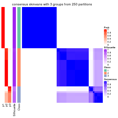
consensus_heatmap(res, k = 4)
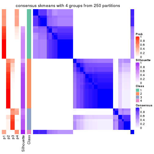
consensus_heatmap(res, k = 5)
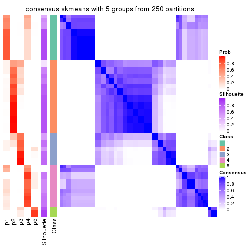
consensus_heatmap(res, k = 6)
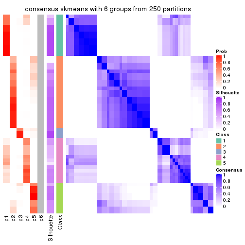
Heatmaps for the membership of samples in all partitions to see how consistent they are:
membership_heatmap(res, k = 2)

membership_heatmap(res, k = 3)
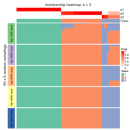
membership_heatmap(res, k = 4)
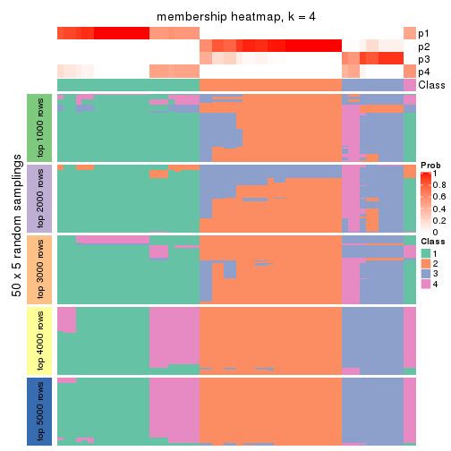
membership_heatmap(res, k = 5)
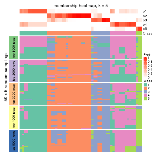
membership_heatmap(res, k = 6)
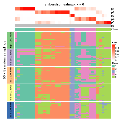
As soon as we have had the classes for columns, we can look for signatures which are significantly different between classes which can be candidate marks for certain classes. Following are the heatmaps for signatures.
Signature heatmaps where rows are scaled:
get_signatures(res, k = 2)

get_signatures(res, k = 3)
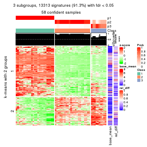
get_signatures(res, k = 4)
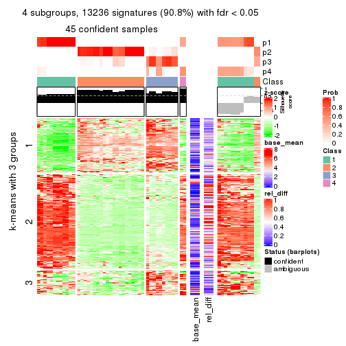
get_signatures(res, k = 5)
get_signatures(res, k = 6)
Signature heatmaps where rows are not scaled:
get_signatures(res, k = 2, scale_rows = FALSE)

get_signatures(res, k = 3, scale_rows = FALSE)
get_signatures(res, k = 4, scale_rows = FALSE)
get_signatures(res, k = 5, scale_rows = FALSE)
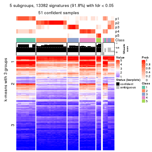
get_signatures(res, k = 6, scale_rows = FALSE)
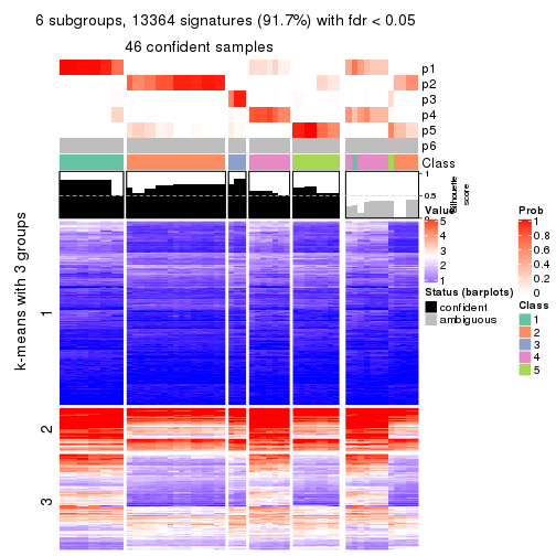
Compare the overlap of signatures from different k:
compare_signatures(res)
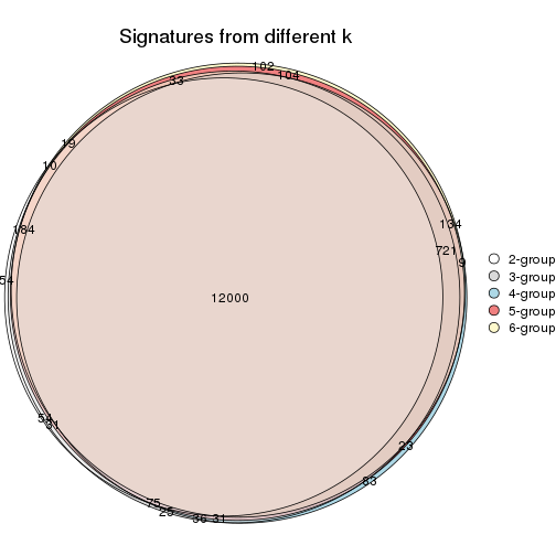
get_signature() returns a data frame invisibly. TO get the list of signatures, the function
call should be assigned to a variable explicitly. In following code, if plot argument is set
to FALSE, no heatmap is plotted while only the differential analysis is performed.
# code only for demonstration
tb = get_signature(res, k = ..., plot = FALSE)
An example of the output of tb is:
#>   which_row         fdr    mean_1    mean_2 scaled_mean_1 scaled_mean_2 km
#> 1        38 0.042760348  8.373488  9.131774    -0.5533452     0.5164555  1
#> 2        40 0.018707592  7.106213  8.469186    -0.6173731     0.5762149  1
#> 3        55 0.019134737 10.221463 11.207825    -0.6159697     0.5749050  1
#> 4        59 0.006059896  5.921854  7.869574    -0.6899429     0.6439467  1
#> 5        60 0.018055526  8.928898 10.211722    -0.6204761     0.5791110  1
#> 6        98 0.009384629 15.714769 14.887706     0.6635654    -0.6193277  2
...
The columns in tb are:
which_row: row indices corresponding to the input matrix.fdr: FDR for the differential test. mean_x: The mean value in group x.scaled_mean_x: The mean value in group x after rows are scaled.km: Row groups if k-means clustering is applied to rows.UMAP plot which shows how samples are separated.
dimension_reduction(res, k = 2, method = "UMAP")

dimension_reduction(res, k = 3, method = "UMAP")
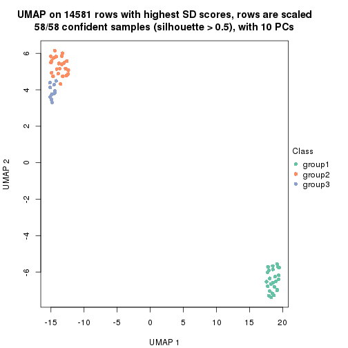
dimension_reduction(res, k = 4, method = "UMAP")
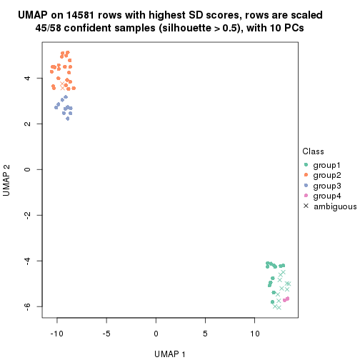
dimension_reduction(res, k = 5, method = "UMAP")
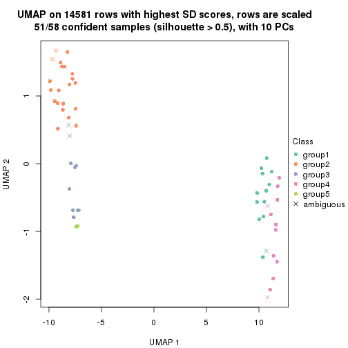
dimension_reduction(res, k = 6, method = "UMAP")
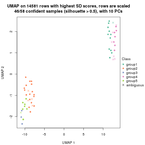
Following heatmap shows how subgroups are split when increasing k:
collect_classes(res)
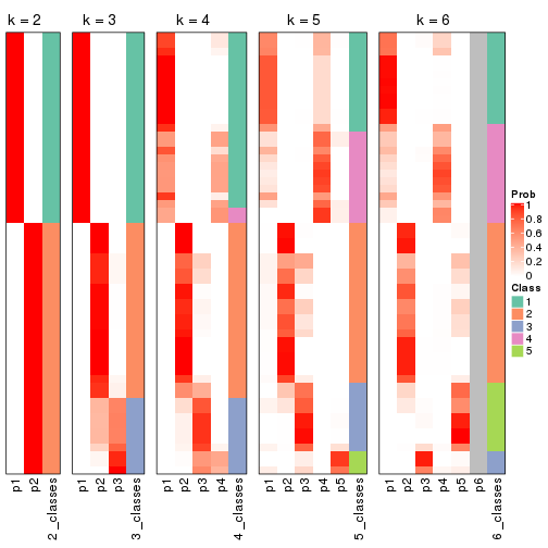
If matrix rows can be associated to genes, consider to use functional_enrichment(res,
...) to perform function enrichment for the signature genes. See this vignette for more detailed explanations.
The object with results only for a single top-value method and a single partition method can be extracted as:
res = res_list["SD", "pam"]
# you can also extract it by
# res = res_list["SD:pam"]
A summary of res and all the functions that can be applied to it:
res
#> A 'ConsensusPartition' object with k = 2, 3, 4, 5, 6.
#>   On a matrix with 14581 rows and 58 columns.
#>   Top rows (1000, 2000, 3000, 4000, 5000) are extracted by 'SD' method.
#>   Subgroups are detected by 'pam' method.
#>   Performed in total 1250 partitions by row resampling.
#>   Best k for subgroups seems to be 2.
#>
#> Following methods can be applied to this 'ConsensusPartition' object:
#>  [1] "cola_report"             "collect_classes"         "collect_plots"
#>  [4] "collect_stats"           "colnames"                "compare_signatures"
#>  [7] "consensus_heatmap"       "dimension_reduction"     "functional_enrichment"
#> [10] "get_anno_col"            "get_anno"                "get_classes"
#> [13] "get_consensus"           "get_matrix"              "get_membership"
#> [16] "get_param"               "get_signatures"          "get_stats"
#> [19] "is_best_k"               "is_stable_k"             "membership_heatmap"
#> [22] "ncol"                    "nrow"                    "plot_ecdf"
#> [25] "rownames"                "select_partition_number" "show"
#> [28] "suggest_best_k"          "test_to_known_factors"
collect_plots() function collects all the plots made from res for all k (number of partitions)
into one single page to provide an easy and fast comparison between different k.
collect_plots(res)
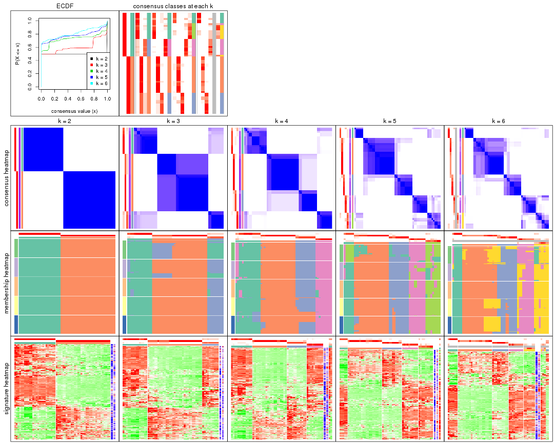
The plots are:
k and the heatmap of
predicted classes for each k.k.k.k.All the plots in panels can be made by individual functions and they are plotted later in this section.
select_partition_number() produces several plots showing different
statistics for choosing “optimized” k. There are following statistics:
k;k, the area increased is defined as \(A_k - A_{k-1}\).The detailed explanations of these statistics can be found in the cola vignette.
Generally speaking, lower PAC score, higher mean silhouette score or higher
concordance corresponds to better partition. Rand index and Jaccard index
measure how similar the current partition is compared to partition with k-1.
If they are too similar, we won't accept k is better than k-1.
select_partition_number(res)
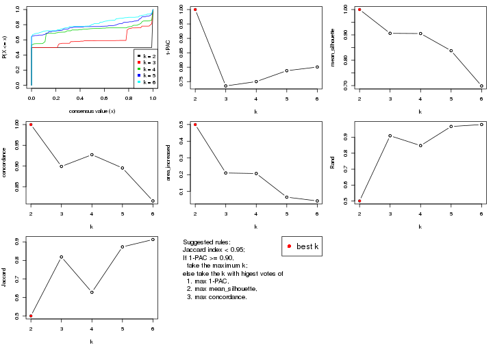
The numeric values for all these statistics can be obtained by get_stats().
get_stats(res)
#>   k 1-PAC mean_silhouette concordance area_increased  Rand Jaccard
#> 2 2 1.000           1.000       1.000         0.4996 0.501   0.501
#> 3 3 0.735           0.906       0.899         0.2102 0.909   0.819
#> 4 4 0.750           0.905       0.927         0.2070 0.848   0.628
#> 5 5 0.788           0.838       0.895         0.0657 0.967   0.873
#> 6 6 0.801           0.699       0.816         0.0433 0.979   0.913
suggest_best_k() suggests the best \(k\) based on these statistics. The rules are as follows:
suggest_best_k(res)
#> [1] 2
Following shows the table of the partitions (You need to click the show/hide
code output link to see it). The membership matrix (columns with name p*)
is inferred by
clue::cl_consensus()
function with the SE method. Basically the value in the membership matrix
represents the probability to belong to a certain group. The finall class
label for an item is determined with the group with highest probability it
belongs to.
In get_classes() function, the entropy is calculated from the membership
matrix and the silhouette score is calculated from the consensus matrix.
cbind(get_classes(res, k = 2), get_membership(res, k = 2))
#>           class entropy silhouette p1 p2
#> ERR789082     2       0          1  0  1
#> ERR789083     2       0          1  0  1
#> ERR789191     2       0          1  0  1
#> ERR789192     2       0          1  0  1
#> ERR789213     1       0          1  1  0
#> ERR789385     1       0          1  1  0
#> ERR789393     1       0          1  1  0
#> ERR789394     1       0          1  1  0
#> ERR789193     2       0          1  0  1
#> ERR789194     2       0          1  0  1
#> ERR789195     2       0          1  0  1
#> ERR789196     2       0          1  0  1
#> ERR789388     1       0          1  1  0
#> ERR789197     2       0          1  0  1
#> ERR789198     2       0          1  0  1
#> ERR789214     1       0          1  1  0
#> ERR789397     1       0          1  1  0
#> ERR789398     1       0          1  1  0
#> ERR789199     2       0          1  0  1
#> ERR789200     2       0          1  0  1
#> ERR789201     2       0          1  0  1
#> ERR789202     2       0          1  0  1
#> ERR789215     1       0          1  1  0
#> ERR789203     2       0          1  0  1
#> ERR789204     2       0          1  0  1
#> ERR789383     1       0          1  1  0
#> ERR789205     2       0          1  0  1
#> ERR789206     2       0          1  0  1
#> ERR789399     1       0          1  1  0
#> ERR789400     1       0          1  1  0
#> ERR789207     2       0          1  0  1
#> ERR789208     2       0          1  0  1
#> ERR789209     2       0          1  0  1
#> ERR789210     2       0          1  0  1
#> ERR789211     2       0          1  0  1
#> ERR789212     2       0          1  0  1
#> ERR789386     1       0          1  1  0
#> ERR789076     2       0          1  0  1
#> ERR789077     2       0          1  0  1
#> ERR789384     1       0          1  1  0
#> ERR789078     2       0          1  0  1
#> ERR789079     2       0          1  0  1
#> ERR789216     1       0          1  1  0
#> ERR789080     2       0          1  0  1
#> ERR789387     1       0          1  1  0
#> ERR789081     2       0          1  0  1
#> ERR789064     2       0          1  0  1
#> ERR779485     2       0          1  0  1
#> ERR789065     2       0          1  0  1
#> ERR789401     1       0          1  1  0
#> ERR789402     1       0          1  1  0
#> ERR789403     1       0          1  1  0
#> ERR789389     1       0          1  1  0
#> ERR789395     1       0          1  1  0
#> ERR789396     1       0          1  1  0
#> ERR789390     1       0          1  1  0
#> ERR789391     1       0          1  1  0
#> ERR789392     1       0          1  1  0
cbind(get_classes(res, k = 3), get_membership(res, k = 3))
#>           class entropy silhouette    p1    p2    p3
#> ERR789082     2  0.0000      0.924 0.000 1.000 0.000
#> ERR789083     2  0.0000      0.924 0.000 1.000 0.000
#> ERR789191     2  0.0000      0.924 0.000 1.000 0.000
#> ERR789192     2  0.0000      0.924 0.000 1.000 0.000
#> ERR789213     3  0.4796      0.969 0.220 0.000 0.780
#> ERR789385     3  0.4796      0.969 0.220 0.000 0.780
#> ERR789393     3  0.4796      0.969 0.220 0.000 0.780
#> ERR789394     3  0.4796      0.969 0.220 0.000 0.780
#> ERR789193     2  0.4796      0.863 0.000 0.780 0.220
#> ERR789194     2  0.4796      0.863 0.000 0.780 0.220
#> ERR789195     2  0.4796      0.863 0.000 0.780 0.220
#> ERR789196     2  0.4796      0.863 0.000 0.780 0.220
#> ERR789388     1  0.4702      0.641 0.788 0.000 0.212
#> ERR789197     2  0.0592      0.921 0.000 0.988 0.012
#> ERR789198     2  0.0000      0.924 0.000 1.000 0.000
#> ERR789214     3  0.4796      0.969 0.220 0.000 0.780
#> ERR789397     1  0.2959      0.845 0.900 0.000 0.100
#> ERR789398     1  0.2959      0.845 0.900 0.000 0.100
#> ERR789199     2  0.0000      0.924 0.000 1.000 0.000
#> ERR789200     2  0.0000      0.924 0.000 1.000 0.000
#> ERR789201     2  0.4796      0.863 0.000 0.780 0.220
#> ERR789202     2  0.4796      0.863 0.000 0.780 0.220
#> ERR789215     1  0.1163      0.918 0.972 0.000 0.028
#> ERR789203     2  0.4796      0.863 0.000 0.780 0.220
#> ERR789204     2  0.4796      0.863 0.000 0.780 0.220
#> ERR789383     1  0.0000      0.938 1.000 0.000 0.000
#> ERR789205     2  0.4796      0.863 0.000 0.780 0.220
#> ERR789206     2  0.4796      0.863 0.000 0.780 0.220
#> ERR789399     1  0.0000      0.938 1.000 0.000 0.000
#> ERR789400     1  0.0000      0.938 1.000 0.000 0.000
#> ERR789207     2  0.0000      0.924 0.000 1.000 0.000
#> ERR789208     2  0.0000      0.924 0.000 1.000 0.000
#> ERR789209     2  0.0000      0.924 0.000 1.000 0.000
#> ERR789210     2  0.0000      0.924 0.000 1.000 0.000
#> ERR789211     2  0.0000      0.924 0.000 1.000 0.000
#> ERR789212     2  0.0000      0.924 0.000 1.000 0.000
#> ERR789386     3  0.5678      0.863 0.316 0.000 0.684
#> ERR789076     2  0.1163      0.918 0.000 0.972 0.028
#> ERR789077     2  0.0000      0.924 0.000 1.000 0.000
#> ERR789384     3  0.4796      0.969 0.220 0.000 0.780
#> ERR789078     2  0.0000      0.924 0.000 1.000 0.000
#> ERR789079     2  0.0000      0.924 0.000 1.000 0.000
#> ERR789216     3  0.4796      0.969 0.220 0.000 0.780
#> ERR789080     2  0.0000      0.924 0.000 1.000 0.000
#> ERR789387     3  0.5706      0.858 0.320 0.000 0.680
#> ERR789081     2  0.0000      0.924 0.000 1.000 0.000
#> ERR789064     2  0.0000      0.924 0.000 1.000 0.000
#> ERR779485     2  0.4796      0.863 0.000 0.780 0.220
#> ERR789065     2  0.4796      0.863 0.000 0.780 0.220
#> ERR789401     1  0.0000      0.938 1.000 0.000 0.000
#> ERR789402     1  0.0000      0.938 1.000 0.000 0.000
#> ERR789403     1  0.0000      0.938 1.000 0.000 0.000
#> ERR789389     1  0.4235      0.716 0.824 0.000 0.176
#> ERR789395     1  0.0000      0.938 1.000 0.000 0.000
#> ERR789396     1  0.0000      0.938 1.000 0.000 0.000
#> ERR789390     1  0.0237      0.937 0.996 0.000 0.004
#> ERR789391     1  0.0237      0.937 0.996 0.000 0.004
#> ERR789392     3  0.4796      0.969 0.220 0.000 0.780
cbind(get_classes(res, k = 4), get_membership(res, k = 4))
#>           class entropy silhouette    p1    p2    p3    p4
#> ERR789082     2  0.0000      0.980 0.000 1.000 0.000 0.000
#> ERR789083     2  0.0000      0.980 0.000 1.000 0.000 0.000
#> ERR789191     2  0.0000      0.980 0.000 1.000 0.000 0.000
#> ERR789192     2  0.0000      0.980 0.000 1.000 0.000 0.000
#> ERR789213     4  0.0000      0.971 0.000 0.000 0.000 1.000
#> ERR789385     4  0.0000      0.971 0.000 0.000 0.000 1.000
#> ERR789393     4  0.0000      0.971 0.000 0.000 0.000 1.000
#> ERR789394     4  0.0000      0.971 0.000 0.000 0.000 1.000
#> ERR789193     3  0.2589      0.959 0.000 0.116 0.884 0.000
#> ERR789194     3  0.2589      0.959 0.000 0.116 0.884 0.000
#> ERR789195     3  0.2589      0.959 0.000 0.116 0.884 0.000
#> ERR789196     3  0.2589      0.959 0.000 0.116 0.884 0.000
#> ERR789388     1  0.4916      0.236 0.576 0.000 0.000 0.424
#> ERR789197     2  0.2345      0.877 0.000 0.900 0.100 0.000
#> ERR789198     2  0.2081      0.894 0.000 0.916 0.084 0.000
#> ERR789214     4  0.0817      0.955 0.024 0.000 0.000 0.976
#> ERR789397     1  0.2469      0.818 0.892 0.000 0.000 0.108
#> ERR789398     1  0.2469      0.818 0.892 0.000 0.000 0.108
#> ERR789199     2  0.0000      0.980 0.000 1.000 0.000 0.000
#> ERR789200     2  0.0000      0.980 0.000 1.000 0.000 0.000
#> ERR789201     3  0.4331      0.780 0.000 0.288 0.712 0.000
#> ERR789202     3  0.4543      0.724 0.000 0.324 0.676 0.000
#> ERR789215     1  0.2345      0.830 0.900 0.000 0.000 0.100
#> ERR789203     3  0.2589      0.959 0.000 0.116 0.884 0.000
#> ERR789204     3  0.2589      0.959 0.000 0.116 0.884 0.000
#> ERR789383     1  0.0817      0.872 0.976 0.000 0.024 0.000
#> ERR789205     3  0.2589      0.959 0.000 0.116 0.884 0.000
#> ERR789206     3  0.2589      0.959 0.000 0.116 0.884 0.000
#> ERR789399     1  0.0000      0.870 1.000 0.000 0.000 0.000
#> ERR789400     1  0.0000      0.870 1.000 0.000 0.000 0.000
#> ERR789207     2  0.0000      0.980 0.000 1.000 0.000 0.000
#> ERR789208     2  0.0000      0.980 0.000 1.000 0.000 0.000
#> ERR789209     2  0.0000      0.980 0.000 1.000 0.000 0.000
#> ERR789210     2  0.0000      0.980 0.000 1.000 0.000 0.000
#> ERR789211     2  0.0000      0.980 0.000 1.000 0.000 0.000
#> ERR789212     2  0.0000      0.980 0.000 1.000 0.000 0.000
#> ERR789386     4  0.2281      0.889 0.096 0.000 0.000 0.904
#> ERR789076     2  0.3219      0.787 0.000 0.836 0.164 0.000
#> ERR789077     2  0.0000      0.980 0.000 1.000 0.000 0.000
#> ERR789384     4  0.0000      0.971 0.000 0.000 0.000 1.000
#> ERR789078     2  0.0000      0.980 0.000 1.000 0.000 0.000
#> ERR789079     2  0.0000      0.980 0.000 1.000 0.000 0.000
#> ERR789216     4  0.0000      0.971 0.000 0.000 0.000 1.000
#> ERR789080     2  0.0000      0.980 0.000 1.000 0.000 0.000
#> ERR789387     4  0.2408      0.881 0.104 0.000 0.000 0.896
#> ERR789081     2  0.0000      0.980 0.000 1.000 0.000 0.000
#> ERR789064     2  0.0000      0.980 0.000 1.000 0.000 0.000
#> ERR779485     3  0.2589      0.959 0.000 0.116 0.884 0.000
#> ERR789065     3  0.2589      0.959 0.000 0.116 0.884 0.000
#> ERR789401     1  0.2589      0.866 0.884 0.000 0.116 0.000
#> ERR789402     1  0.2589      0.866 0.884 0.000 0.116 0.000
#> ERR789403     1  0.2589      0.866 0.884 0.000 0.116 0.000
#> ERR789389     1  0.6961      0.315 0.496 0.000 0.116 0.388
#> ERR789395     1  0.2589      0.866 0.884 0.000 0.116 0.000
#> ERR789396     1  0.2589      0.866 0.884 0.000 0.116 0.000
#> ERR789390     1  0.0469      0.870 0.988 0.000 0.000 0.012
#> ERR789391     1  0.0469      0.870 0.988 0.000 0.000 0.012
#> ERR789392     4  0.0000      0.971 0.000 0.000 0.000 1.000
cbind(get_classes(res, k = 5), get_membership(res, k = 5))
#>           class entropy silhouette    p1    p2    p3    p4    p5
#> ERR789082     2  0.0404      0.937 0.012 0.988 0.000 0.000 0.000
#> ERR789083     2  0.0290      0.938 0.008 0.992 0.000 0.000 0.000
#> ERR789191     2  0.0000      0.939 0.000 1.000 0.000 0.000 0.000
#> ERR789192     2  0.0404      0.937 0.012 0.988 0.000 0.000 0.000
#> ERR789213     4  0.1197      0.913 0.000 0.000 0.000 0.952 0.048
#> ERR789385     4  0.1341      0.914 0.000 0.000 0.000 0.944 0.056
#> ERR789393     4  0.1341      0.914 0.000 0.000 0.000 0.944 0.056
#> ERR789394     4  0.1341      0.914 0.000 0.000 0.000 0.944 0.056
#> ERR789193     3  0.0703      0.896 0.024 0.000 0.976 0.000 0.000
#> ERR789194     3  0.0703      0.896 0.024 0.000 0.976 0.000 0.000
#> ERR789195     3  0.2230      0.836 0.116 0.000 0.884 0.000 0.000
#> ERR789196     3  0.2230      0.836 0.116 0.000 0.884 0.000 0.000
#> ERR789388     5  0.4243      0.555 0.024 0.000 0.000 0.264 0.712
#> ERR789197     2  0.4588      0.779 0.116 0.748 0.136 0.000 0.000
#> ERR789198     2  0.4588      0.779 0.116 0.748 0.136 0.000 0.000
#> ERR789214     4  0.3366      0.655 0.000 0.000 0.000 0.768 0.232
#> ERR789397     5  0.2179      0.722 0.000 0.000 0.000 0.112 0.888
#> ERR789398     5  0.2179      0.722 0.000 0.000 0.000 0.112 0.888
#> ERR789199     2  0.2230      0.902 0.116 0.884 0.000 0.000 0.000
#> ERR789200     2  0.2230      0.902 0.116 0.884 0.000 0.000 0.000
#> ERR789201     3  0.3534      0.656 0.000 0.256 0.744 0.000 0.000
#> ERR789202     3  0.3837      0.578 0.000 0.308 0.692 0.000 0.000
#> ERR789215     5  0.3895      0.567 0.000 0.000 0.000 0.320 0.680
#> ERR789203     3  0.0000      0.901 0.000 0.000 1.000 0.000 0.000
#> ERR789204     3  0.0000      0.901 0.000 0.000 1.000 0.000 0.000
#> ERR789383     5  0.3730      0.552 0.288 0.000 0.000 0.000 0.712
#> ERR789205     3  0.0000      0.901 0.000 0.000 1.000 0.000 0.000
#> ERR789206     3  0.0000      0.901 0.000 0.000 1.000 0.000 0.000
#> ERR789399     5  0.3074      0.678 0.196 0.000 0.000 0.000 0.804
#> ERR789400     5  0.3074      0.678 0.196 0.000 0.000 0.000 0.804
#> ERR789207     2  0.0000      0.939 0.000 1.000 0.000 0.000 0.000
#> ERR789208     2  0.0000      0.939 0.000 1.000 0.000 0.000 0.000
#> ERR789209     2  0.0000      0.939 0.000 1.000 0.000 0.000 0.000
#> ERR789210     2  0.0000      0.939 0.000 1.000 0.000 0.000 0.000
#> ERR789211     2  0.0000      0.939 0.000 1.000 0.000 0.000 0.000
#> ERR789212     2  0.0000      0.939 0.000 1.000 0.000 0.000 0.000
#> ERR789386     4  0.2179      0.827 0.000 0.000 0.000 0.888 0.112
#> ERR789076     2  0.4967      0.712 0.104 0.704 0.192 0.000 0.000
#> ERR789077     2  0.2020      0.909 0.100 0.900 0.000 0.000 0.000
#> ERR789384     4  0.0000      0.901 0.000 0.000 0.000 1.000 0.000
#> ERR789078     2  0.1965      0.911 0.096 0.904 0.000 0.000 0.000
#> ERR789079     2  0.0000      0.939 0.000 1.000 0.000 0.000 0.000
#> ERR789216     4  0.0000      0.901 0.000 0.000 0.000 1.000 0.000
#> ERR789080     2  0.0000      0.939 0.000 1.000 0.000 0.000 0.000
#> ERR789387     4  0.2179      0.827 0.000 0.000 0.000 0.888 0.112
#> ERR789081     2  0.0000      0.939 0.000 1.000 0.000 0.000 0.000
#> ERR789064     2  0.2077      0.914 0.084 0.908 0.008 0.000 0.000
#> ERR779485     3  0.0703      0.896 0.024 0.000 0.976 0.000 0.000
#> ERR789065     3  0.0000      0.901 0.000 0.000 1.000 0.000 0.000
#> ERR789401     1  0.2516      0.886 0.860 0.000 0.000 0.000 0.140
#> ERR789402     1  0.2516      0.886 0.860 0.000 0.000 0.000 0.140
#> ERR789403     1  0.2516      0.886 0.860 0.000 0.000 0.000 0.140
#> ERR789389     1  0.4211      0.382 0.636 0.000 0.000 0.360 0.004
#> ERR789395     1  0.2516      0.886 0.860 0.000 0.000 0.000 0.140
#> ERR789396     1  0.2516      0.886 0.860 0.000 0.000 0.000 0.140
#> ERR789390     5  0.0000      0.756 0.000 0.000 0.000 0.000 1.000
#> ERR789391     5  0.0000      0.756 0.000 0.000 0.000 0.000 1.000
#> ERR789392     4  0.1341      0.914 0.000 0.000 0.000 0.944 0.056
cbind(get_classes(res, k = 6), get_membership(res, k = 6))
#>           class entropy silhouette    p1    p2    p3    p4 p5    p6
#> ERR789082     2  0.2362      0.723 0.000 0.860 0.004 0.000 NA 0.000
#> ERR789083     2  0.2402      0.723 0.000 0.856 0.004 0.000 NA 0.000
#> ERR789191     2  0.3828      0.817 0.000 0.560 0.000 0.000 NA 0.000
#> ERR789192     2  0.3789      0.815 0.000 0.584 0.000 0.000 NA 0.000
#> ERR789213     4  0.3998      0.792 0.000 0.000 0.000 0.644 NA 0.016
#> ERR789385     4  0.4224      0.793 0.000 0.000 0.000 0.632 NA 0.028
#> ERR789393     4  0.4224      0.793 0.000 0.000 0.000 0.632 NA 0.028
#> ERR789394     4  0.4224      0.793 0.000 0.000 0.000 0.632 NA 0.028
#> ERR789193     3  0.1285      0.819 0.000 0.000 0.944 0.000 NA 0.004
#> ERR789194     3  0.1285      0.819 0.000 0.000 0.944 0.000 NA 0.004
#> ERR789195     3  0.3961      0.499 0.000 0.440 0.556 0.000 NA 0.000
#> ERR789196     3  0.3961      0.499 0.000 0.440 0.556 0.000 NA 0.000
#> ERR789388     6  0.1863      0.525 0.000 0.000 0.000 0.104 NA 0.896
#> ERR789197     2  0.1531      0.597 0.000 0.928 0.068 0.000 NA 0.000
#> ERR789198     2  0.1531      0.597 0.000 0.928 0.068 0.000 NA 0.000
#> ERR789214     6  0.3578      0.154 0.000 0.000 0.000 0.340 NA 0.660
#> ERR789397     6  0.1349      0.547 0.004 0.000 0.000 0.000 NA 0.940
#> ERR789398     6  0.1349      0.547 0.004 0.000 0.000 0.000 NA 0.940
#> ERR789199     2  0.0000      0.666 0.000 1.000 0.000 0.000 NA 0.000
#> ERR789200     2  0.0000      0.666 0.000 1.000 0.000 0.000 NA 0.000
#> ERR789201     3  0.3803      0.658 0.000 0.056 0.760 0.000 NA 0.000
#> ERR789202     3  0.4431      0.589 0.000 0.080 0.692 0.000 NA 0.000
#> ERR789215     4  0.5718     -0.431 0.004 0.000 0.000 0.520 NA 0.308
#> ERR789203     3  0.0000      0.833 0.000 0.000 1.000 0.000 NA 0.000
#> ERR789204     3  0.0000      0.833 0.000 0.000 1.000 0.000 NA 0.000
#> ERR789383     6  0.7612      0.483 0.252 0.000 0.000 0.272 NA 0.308
#> ERR789205     3  0.0000      0.833 0.000 0.000 1.000 0.000 NA 0.000
#> ERR789206     3  0.0000      0.833 0.000 0.000 1.000 0.000 NA 0.000
#> ERR789399     6  0.7523      0.534 0.208 0.000 0.000 0.272 NA 0.352
#> ERR789400     6  0.7523      0.534 0.208 0.000 0.000 0.272 NA 0.352
#> ERR789207     2  0.3828      0.817 0.000 0.560 0.000 0.000 NA 0.000
#> ERR789208     2  0.3828      0.817 0.000 0.560 0.000 0.000 NA 0.000
#> ERR789209     2  0.3828      0.817 0.000 0.560 0.000 0.000 NA 0.000
#> ERR789210     2  0.3828      0.817 0.000 0.560 0.000 0.000 NA 0.000
#> ERR789211     2  0.3828      0.817 0.000 0.560 0.000 0.000 NA 0.000
#> ERR789212     2  0.3828      0.817 0.000 0.560 0.000 0.000 NA 0.000
#> ERR789386     4  0.0260      0.559 0.000 0.000 0.000 0.992 NA 0.008
#> ERR789076     2  0.2383      0.578 0.000 0.880 0.096 0.000 NA 0.000
#> ERR789077     2  0.3499      0.790 0.000 0.680 0.000 0.000 NA 0.000
#> ERR789384     4  0.3266      0.771 0.000 0.000 0.000 0.728 NA 0.000
#> ERR789078     2  0.3531      0.792 0.000 0.672 0.000 0.000 NA 0.000
#> ERR789079     2  0.3828      0.817 0.000 0.560 0.000 0.000 NA 0.000
#> ERR789216     4  0.3266      0.771 0.000 0.000 0.000 0.728 NA 0.000
#> ERR789080     2  0.3828      0.817 0.000 0.560 0.000 0.000 NA 0.000
#> ERR789387     4  0.0260      0.557 0.000 0.000 0.000 0.992 NA 0.000
#> ERR789081     2  0.3828      0.817 0.000 0.560 0.000 0.000 NA 0.000
#> ERR789064     2  0.1124      0.681 0.000 0.956 0.008 0.000 NA 0.000
#> ERR779485     3  0.1219      0.818 0.000 0.000 0.948 0.000 NA 0.004
#> ERR789065     3  0.0146      0.832 0.000 0.000 0.996 0.000 NA 0.000
#> ERR789401     1  0.0000      0.920 1.000 0.000 0.000 0.000 NA 0.000
#> ERR789402     1  0.0000      0.920 1.000 0.000 0.000 0.000 NA 0.000
#> ERR789403     1  0.0000      0.920 1.000 0.000 0.000 0.000 NA 0.000
#> ERR789389     1  0.3464      0.540 0.688 0.000 0.000 0.312 NA 0.000
#> ERR789395     1  0.0000      0.920 1.000 0.000 0.000 0.000 NA 0.000
#> ERR789396     1  0.0000      0.920 1.000 0.000 0.000 0.000 NA 0.000
#> ERR789390     6  0.5578      0.604 0.004 0.000 0.000 0.268 NA 0.560
#> ERR789391     6  0.5550      0.604 0.004 0.000 0.000 0.268 NA 0.564
#> ERR789392     4  0.4224      0.793 0.000 0.000 0.000 0.632 NA 0.028
Heatmaps for the consensus matrix. It visualizes the probability of two samples to be in a same group.
consensus_heatmap(res, k = 2)

consensus_heatmap(res, k = 3)
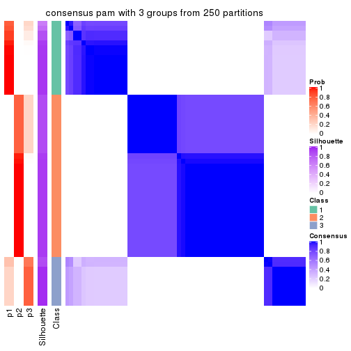
consensus_heatmap(res, k = 4)
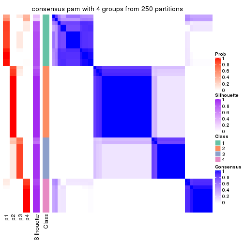
consensus_heatmap(res, k = 5)
consensus_heatmap(res, k = 6)
Heatmaps for the membership of samples in all partitions to see how consistent they are:
membership_heatmap(res, k = 2)

membership_heatmap(res, k = 3)
membership_heatmap(res, k = 4)
membership_heatmap(res, k = 5)
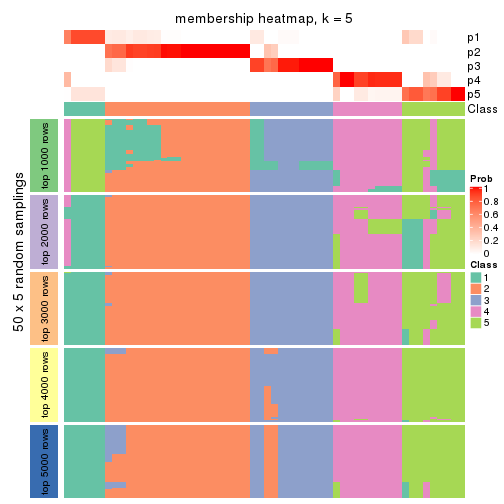
membership_heatmap(res, k = 6)
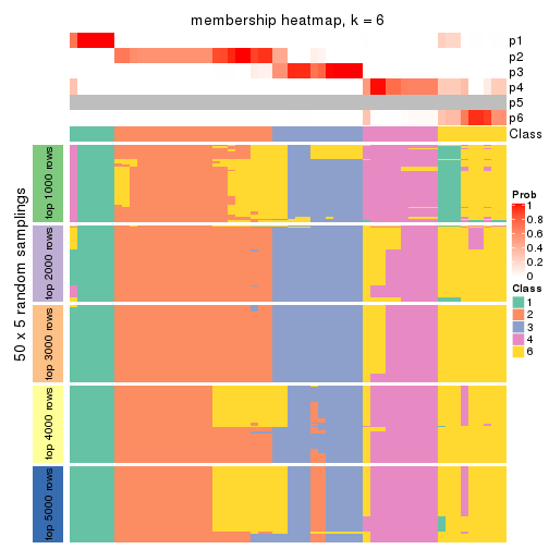
As soon as we have had the classes for columns, we can look for signatures which are significantly different between classes which can be candidate marks for certain classes. Following are the heatmaps for signatures.
Signature heatmaps where rows are scaled:
get_signatures(res, k = 2)

get_signatures(res, k = 3)
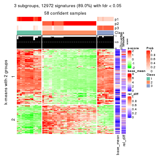
get_signatures(res, k = 4)
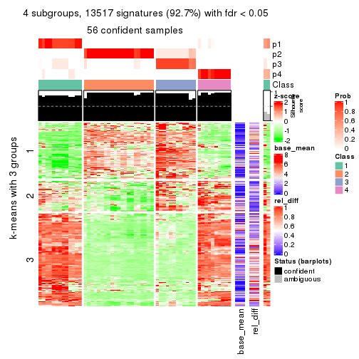
get_signatures(res, k = 5)
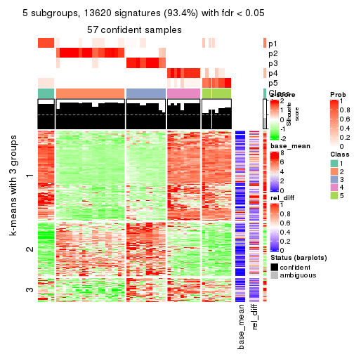
get_signatures(res, k = 6)
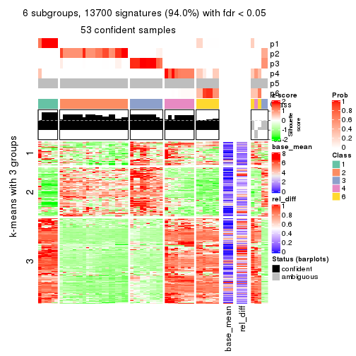
Signature heatmaps where rows are not scaled:
get_signatures(res, k = 2, scale_rows = FALSE)

get_signatures(res, k = 3, scale_rows = FALSE)
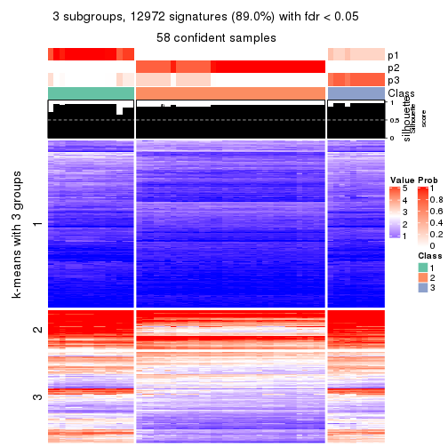
get_signatures(res, k = 4, scale_rows = FALSE)
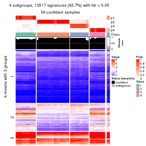
get_signatures(res, k = 5, scale_rows = FALSE)
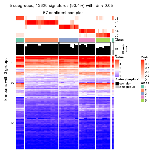
get_signatures(res, k = 6, scale_rows = FALSE)
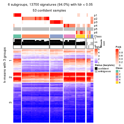
Compare the overlap of signatures from different k:
compare_signatures(res)
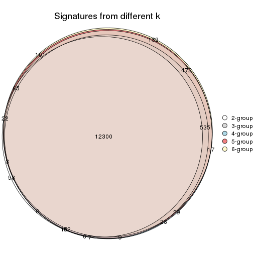
get_signature() returns a data frame invisibly. TO get the list of signatures, the function
call should be assigned to a variable explicitly. In following code, if plot argument is set
to FALSE, no heatmap is plotted while only the differential analysis is performed.
# code only for demonstration
tb = get_signature(res, k = ..., plot = FALSE)
An example of the output of tb is:
#>   which_row         fdr    mean_1    mean_2 scaled_mean_1 scaled_mean_2 km
#> 1        38 0.042760348  8.373488  9.131774    -0.5533452     0.5164555  1
#> 2        40 0.018707592  7.106213  8.469186    -0.6173731     0.5762149  1
#> 3        55 0.019134737 10.221463 11.207825    -0.6159697     0.5749050  1
#> 4        59 0.006059896  5.921854  7.869574    -0.6899429     0.6439467  1
#> 5        60 0.018055526  8.928898 10.211722    -0.6204761     0.5791110  1
#> 6        98 0.009384629 15.714769 14.887706     0.6635654    -0.6193277  2
...
The columns in tb are:
which_row: row indices corresponding to the input matrix.fdr: FDR for the differential test. mean_x: The mean value in group x.scaled_mean_x: The mean value in group x after rows are scaled.km: Row groups if k-means clustering is applied to rows.UMAP plot which shows how samples are separated.
dimension_reduction(res, k = 2, method = "UMAP")

dimension_reduction(res, k = 3, method = "UMAP")
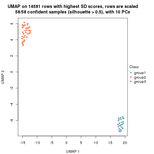
dimension_reduction(res, k = 4, method = "UMAP")
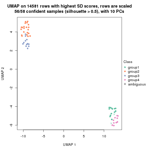
dimension_reduction(res, k = 5, method = "UMAP")
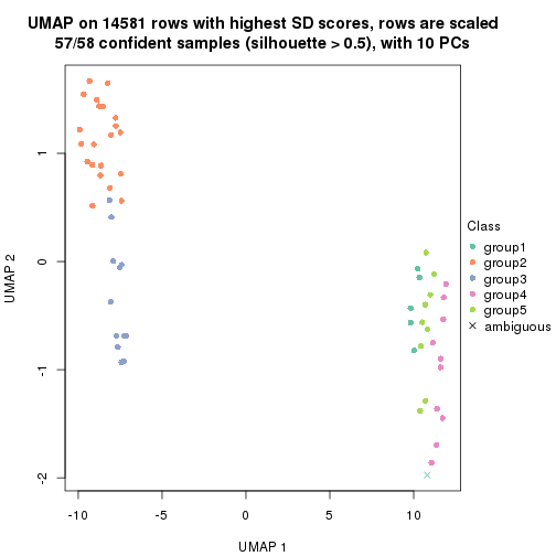
dimension_reduction(res, k = 6, method = "UMAP")
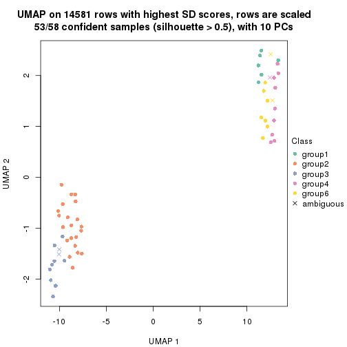
Following heatmap shows how subgroups are split when increasing k:
collect_classes(res)
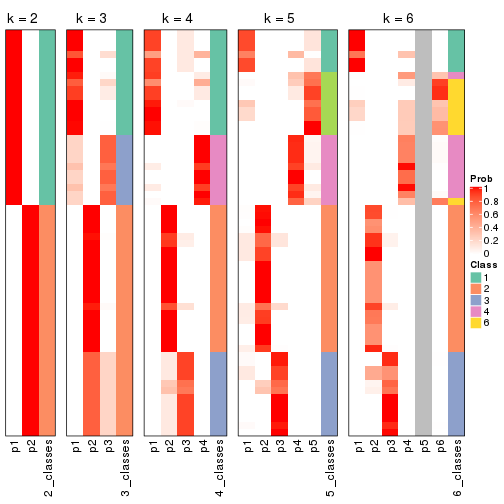
If matrix rows can be associated to genes, consider to use functional_enrichment(res,
...) to perform function enrichment for the signature genes. See this vignette for more detailed explanations.
The object with results only for a single top-value method and a single partition method can be extracted as:
res = res_list["SD", "mclust"]
# you can also extract it by
# res = res_list["SD:mclust"]
A summary of res and all the functions that can be applied to it:
res
#> A 'ConsensusPartition' object with k = 2, 3, 4, 5, 6.
#>   On a matrix with 14581 rows and 58 columns.
#>   Top rows (1000, 2000, 3000, 4000, 5000) are extracted by 'SD' method.
#>   Subgroups are detected by 'mclust' method.
#>   Performed in total 1250 partitions by row resampling.
#>   Best k for subgroups seems to be 2.
#>
#> Following methods can be applied to this 'ConsensusPartition' object:
#>  [1] "cola_report"             "collect_classes"         "collect_plots"
#>  [4] "collect_stats"           "colnames"                "compare_signatures"
#>  [7] "consensus_heatmap"       "dimension_reduction"     "functional_enrichment"
#> [10] "get_anno_col"            "get_anno"                "get_classes"
#> [13] "get_consensus"           "get_matrix"              "get_membership"
#> [16] "get_param"               "get_signatures"          "get_stats"
#> [19] "is_best_k"               "is_stable_k"             "membership_heatmap"
#> [22] "ncol"                    "nrow"                    "plot_ecdf"
#> [25] "rownames"                "select_partition_number" "show"
#> [28] "suggest_best_k"          "test_to_known_factors"
collect_plots() function collects all the plots made from res for all k (number of partitions)
into one single page to provide an easy and fast comparison between different k.
collect_plots(res)
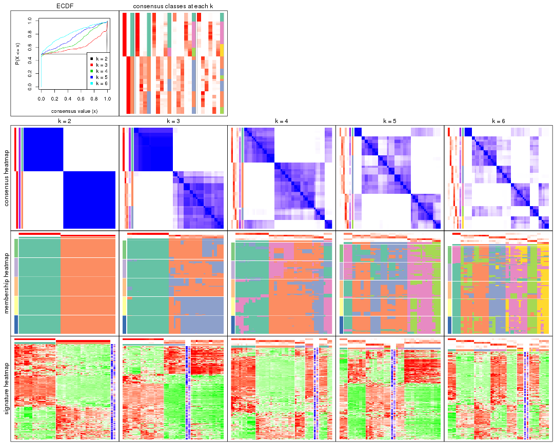
The plots are:
k and the heatmap of
predicted classes for each k.k.k.k.All the plots in panels can be made by individual functions and they are plotted later in this section.
select_partition_number() produces several plots showing different
statistics for choosing “optimized” k. There are following statistics:
k;k, the area increased is defined as \(A_k - A_{k-1}\).The detailed explanations of these statistics can be found in the cola vignette.
Generally speaking, lower PAC score, higher mean silhouette score or higher
concordance corresponds to better partition. Rand index and Jaccard index
measure how similar the current partition is compared to partition with k-1.
If they are too similar, we won't accept k is better than k-1.
select_partition_number(res)
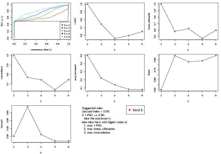
The numeric values for all these statistics can be obtained by get_stats().
get_stats(res)
#>   k 1-PAC mean_silhouette concordance area_increased  Rand Jaccard
#> 2 2 1.000           1.000       1.000         0.4996 0.501   0.501
#> 3 3 0.745           0.583       0.771         0.2222 0.843   0.686
#> 4 4 0.562           0.624       0.744         0.1387 0.782   0.512
#> 5 5 0.596           0.474       0.640         0.0835 0.791   0.470
#> 6 6 0.649           0.599       0.745         0.0789 0.844   0.470
suggest_best_k() suggests the best \(k\) based on these statistics. The rules are as follows:
suggest_best_k(res)
#> [1] 2
Following shows the table of the partitions (You need to click the show/hide
code output link to see it). The membership matrix (columns with name p*)
is inferred by
clue::cl_consensus()
function with the SE method. Basically the value in the membership matrix
represents the probability to belong to a certain group. The finall class
label for an item is determined with the group with highest probability it
belongs to.
In get_classes() function, the entropy is calculated from the membership
matrix and the silhouette score is calculated from the consensus matrix.
cbind(get_classes(res, k = 2), get_membership(res, k = 2))
#>           class entropy silhouette p1 p2
#> ERR789082     2       0          1  0  1
#> ERR789083     2       0          1  0  1
#> ERR789191     2       0          1  0  1
#> ERR789192     2       0          1  0  1
#> ERR789213     1       0          1  1  0
#> ERR789385     1       0          1  1  0
#> ERR789393     1       0          1  1  0
#> ERR789394     1       0          1  1  0
#> ERR789193     2       0          1  0  1
#> ERR789194     2       0          1  0  1
#> ERR789195     2       0          1  0  1
#> ERR789196     2       0          1  0  1
#> ERR789388     1       0          1  1  0
#> ERR789197     2       0          1  0  1
#> ERR789198     2       0          1  0  1
#> ERR789214     1       0          1  1  0
#> ERR789397     1       0          1  1  0
#> ERR789398     1       0          1  1  0
#> ERR789199     2       0          1  0  1
#> ERR789200     2       0          1  0  1
#> ERR789201     2       0          1  0  1
#> ERR789202     2       0          1  0  1
#> ERR789215     1       0          1  1  0
#> ERR789203     2       0          1  0  1
#> ERR789204     2       0          1  0  1
#> ERR789383     1       0          1  1  0
#> ERR789205     2       0          1  0  1
#> ERR789206     2       0          1  0  1
#> ERR789399     1       0          1  1  0
#> ERR789400     1       0          1  1  0
#> ERR789207     2       0          1  0  1
#> ERR789208     2       0          1  0  1
#> ERR789209     2       0          1  0  1
#> ERR789210     2       0          1  0  1
#> ERR789211     2       0          1  0  1
#> ERR789212     2       0          1  0  1
#> ERR789386     1       0          1  1  0
#> ERR789076     2       0          1  0  1
#> ERR789077     2       0          1  0  1
#> ERR789384     1       0          1  1  0
#> ERR789078     2       0          1  0  1
#> ERR789079     2       0          1  0  1
#> ERR789216     1       0          1  1  0
#> ERR789080     2       0          1  0  1
#> ERR789387     1       0          1  1  0
#> ERR789081     2       0          1  0  1
#> ERR789064     2       0          1  0  1
#> ERR779485     2       0          1  0  1
#> ERR789065     2       0          1  0  1
#> ERR789401     1       0          1  1  0
#> ERR789402     1       0          1  1  0
#> ERR789403     1       0          1  1  0
#> ERR789389     1       0          1  1  0
#> ERR789395     1       0          1  1  0
#> ERR789396     1       0          1  1  0
#> ERR789390     1       0          1  1  0
#> ERR789391     1       0          1  1  0
#> ERR789392     1       0          1  1  0
cbind(get_classes(res, k = 3), get_membership(res, k = 3))
#>           class entropy silhouette    p1    p2    p3
#> ERR789082     2  0.6280    -0.2208 0.000 0.540 0.460
#> ERR789083     2  0.6274    -0.2163 0.000 0.544 0.456
#> ERR789191     3  0.6095     0.6004 0.000 0.392 0.608
#> ERR789192     3  0.6095     0.6004 0.000 0.392 0.608
#> ERR789213     1  0.0892     0.9807 0.980 0.000 0.020
#> ERR789385     1  0.0892     0.9807 0.980 0.000 0.020
#> ERR789393     1  0.2796     0.9324 0.908 0.000 0.092
#> ERR789394     1  0.2796     0.9324 0.908 0.000 0.092
#> ERR789193     2  0.5431     0.2420 0.000 0.716 0.284
#> ERR789194     2  0.5431     0.2420 0.000 0.716 0.284
#> ERR789195     2  0.0424     0.3134 0.000 0.992 0.008
#> ERR789196     2  0.0424     0.3134 0.000 0.992 0.008
#> ERR789388     1  0.0237     0.9879 0.996 0.000 0.004
#> ERR789197     2  0.6280    -0.2387 0.000 0.540 0.460
#> ERR789198     2  0.6274    -0.2276 0.000 0.544 0.456
#> ERR789214     1  0.0237     0.9879 0.996 0.000 0.004
#> ERR789397     1  0.0237     0.9879 0.996 0.000 0.004
#> ERR789398     1  0.0237     0.9879 0.996 0.000 0.004
#> ERR789199     2  0.5760     0.1318 0.000 0.672 0.328
#> ERR789200     2  0.5760     0.1318 0.000 0.672 0.328
#> ERR789201     2  0.6274    -0.2237 0.000 0.544 0.456
#> ERR789202     2  0.6274    -0.2237 0.000 0.544 0.456
#> ERR789215     1  0.0000     0.9888 1.000 0.000 0.000
#> ERR789203     2  0.6111     0.0195 0.000 0.604 0.396
#> ERR789204     2  0.6111     0.0195 0.000 0.604 0.396
#> ERR789383     1  0.0237     0.9872 0.996 0.000 0.004
#> ERR789205     2  0.6079     0.0371 0.000 0.612 0.388
#> ERR789206     2  0.6045     0.0506 0.000 0.620 0.380
#> ERR789399     1  0.0000     0.9888 1.000 0.000 0.000
#> ERR789400     1  0.0000     0.9888 1.000 0.000 0.000
#> ERR789207     3  0.5859     0.7100 0.000 0.344 0.656
#> ERR789208     3  0.5859     0.7100 0.000 0.344 0.656
#> ERR789209     3  0.6008     0.6901 0.000 0.372 0.628
#> ERR789210     3  0.5988     0.6920 0.000 0.368 0.632
#> ERR789211     3  0.6204     0.6161 0.000 0.424 0.576
#> ERR789212     3  0.6192     0.6245 0.000 0.420 0.580
#> ERR789386     1  0.0000     0.9888 1.000 0.000 0.000
#> ERR789076     2  0.5058     0.2094 0.000 0.756 0.244
#> ERR789077     3  0.6062     0.6032 0.000 0.384 0.616
#> ERR789384     1  0.0424     0.9865 0.992 0.000 0.008
#> ERR789078     3  0.6062     0.6032 0.000 0.384 0.616
#> ERR789079     3  0.4974     0.6656 0.000 0.236 0.764
#> ERR789216     1  0.0000     0.9888 1.000 0.000 0.000
#> ERR789080     3  0.5785     0.6527 0.000 0.332 0.668
#> ERR789387     1  0.0000     0.9888 1.000 0.000 0.000
#> ERR789081     3  0.4974     0.6656 0.000 0.236 0.764
#> ERR789064     2  0.6111    -0.0849 0.000 0.604 0.396
#> ERR779485     2  0.4931     0.2513 0.000 0.768 0.232
#> ERR789065     2  0.0000     0.3127 0.000 1.000 0.000
#> ERR789401     1  0.0000     0.9888 1.000 0.000 0.000
#> ERR789402     1  0.0000     0.9888 1.000 0.000 0.000
#> ERR789403     1  0.0000     0.9888 1.000 0.000 0.000
#> ERR789389     1  0.0000     0.9888 1.000 0.000 0.000
#> ERR789395     1  0.0000     0.9888 1.000 0.000 0.000
#> ERR789396     1  0.0000     0.9888 1.000 0.000 0.000
#> ERR789390     1  0.0000     0.9888 1.000 0.000 0.000
#> ERR789391     1  0.0000     0.9888 1.000 0.000 0.000
#> ERR789392     1  0.2796     0.9324 0.908 0.000 0.092
cbind(get_classes(res, k = 4), get_membership(res, k = 4))
#>           class entropy silhouette    p1    p2    p3    p4
#> ERR789082     2   0.639     0.6114 0.000 0.636 0.244 0.120
#> ERR789083     2   0.639     0.6114 0.000 0.636 0.244 0.120
#> ERR789191     2   0.523     0.6484 0.000 0.756 0.120 0.124
#> ERR789192     2   0.523     0.6484 0.000 0.756 0.120 0.124
#> ERR789213     4   0.514     0.8342 0.360 0.000 0.012 0.628
#> ERR789385     4   0.513     0.9300 0.312 0.000 0.020 0.668
#> ERR789393     4   0.441     0.9486 0.300 0.000 0.000 0.700
#> ERR789394     4   0.441     0.9486 0.300 0.000 0.000 0.700
#> ERR789193     3   0.297     0.6898 0.000 0.036 0.892 0.072
#> ERR789194     3   0.297     0.6898 0.000 0.036 0.892 0.072
#> ERR789195     3   0.361     0.6883 0.000 0.200 0.800 0.000
#> ERR789196     3   0.361     0.6883 0.000 0.200 0.800 0.000
#> ERR789388     1   0.353     0.6258 0.808 0.000 0.000 0.192
#> ERR789197     2   0.453     0.6556 0.000 0.704 0.292 0.004
#> ERR789198     2   0.456     0.6529 0.000 0.700 0.296 0.004
#> ERR789214     1   0.514     0.1873 0.628 0.000 0.012 0.360
#> ERR789397     1   0.488    -0.0231 0.592 0.000 0.000 0.408
#> ERR789398     1   0.488    -0.0231 0.592 0.000 0.000 0.408
#> ERR789199     2   0.536     0.5870 0.000 0.652 0.320 0.028
#> ERR789200     2   0.536     0.5870 0.000 0.652 0.320 0.028
#> ERR789201     2   0.504     0.6560 0.000 0.744 0.204 0.052
#> ERR789202     2   0.504     0.6560 0.000 0.744 0.204 0.052
#> ERR789215     1   0.417     0.6666 0.816 0.000 0.044 0.140
#> ERR789203     2   0.574     0.5152 0.000 0.628 0.328 0.044
#> ERR789204     2   0.574     0.5152 0.000 0.628 0.328 0.044
#> ERR789383     1   0.220     0.7286 0.928 0.000 0.048 0.024
#> ERR789205     2   0.582     0.4746 0.000 0.608 0.348 0.044
#> ERR789206     2   0.584     0.4682 0.000 0.604 0.352 0.044
#> ERR789399     1   0.100     0.7355 0.972 0.000 0.024 0.004
#> ERR789400     1   0.100     0.7355 0.972 0.000 0.024 0.004
#> ERR789207     2   0.141     0.6830 0.000 0.960 0.016 0.024
#> ERR789208     2   0.141     0.6830 0.000 0.960 0.016 0.024
#> ERR789209     2   0.306     0.6851 0.000 0.888 0.072 0.040
#> ERR789210     2   0.291     0.6877 0.000 0.896 0.064 0.040
#> ERR789211     2   0.320     0.6837 0.000 0.880 0.080 0.040
#> ERR789212     2   0.313     0.6854 0.000 0.884 0.076 0.040
#> ERR789386     1   0.360     0.6962 0.848 0.000 0.028 0.124
#> ERR789076     3   0.632    -0.2840 0.000 0.436 0.504 0.060
#> ERR789077     2   0.538     0.6397 0.000 0.744 0.128 0.128
#> ERR789384     1   0.461     0.5339 0.724 0.000 0.012 0.264
#> ERR789078     2   0.538     0.6397 0.000 0.744 0.128 0.128
#> ERR789079     2   0.389     0.6324 0.000 0.844 0.068 0.088
#> ERR789216     1   0.360     0.6969 0.848 0.000 0.028 0.124
#> ERR789080     2   0.463     0.6577 0.000 0.796 0.124 0.080
#> ERR789387     1   0.305     0.7145 0.884 0.000 0.028 0.088
#> ERR789081     2   0.389     0.6324 0.000 0.844 0.068 0.088
#> ERR789064     2   0.495     0.6433 0.000 0.708 0.268 0.024
#> ERR779485     3   0.240     0.6998 0.000 0.048 0.920 0.032
#> ERR789065     3   0.391     0.6801 0.000 0.212 0.784 0.004
#> ERR789401     1   0.179     0.7147 0.932 0.000 0.000 0.068
#> ERR789402     1   0.179     0.7168 0.932 0.000 0.000 0.068
#> ERR789403     1   0.179     0.7147 0.932 0.000 0.000 0.068
#> ERR789389     1   0.324     0.7211 0.872 0.000 0.028 0.100
#> ERR789395     1   0.179     0.7168 0.932 0.000 0.000 0.068
#> ERR789396     1   0.179     0.7168 0.932 0.000 0.000 0.068
#> ERR789390     1   0.422     0.4536 0.748 0.000 0.004 0.248
#> ERR789391     1   0.422     0.4536 0.748 0.000 0.004 0.248
#> ERR789392     4   0.441     0.9486 0.300 0.000 0.000 0.700
cbind(get_classes(res, k = 5), get_membership(res, k = 5))
#>           class entropy silhouette    p1    p2    p3    p4    p5
#> ERR789082     2  0.5879     0.5044 0.024 0.492 0.436 0.000 0.048
#> ERR789083     2  0.5879     0.5044 0.024 0.492 0.436 0.000 0.048
#> ERR789191     2  0.5265     0.7677 0.024 0.676 0.252 0.000 0.048
#> ERR789192     2  0.5265     0.7677 0.024 0.676 0.252 0.000 0.048
#> ERR789213     5  0.4597     0.3941 0.012 0.000 0.000 0.424 0.564
#> ERR789385     5  0.3942     0.7237 0.012 0.000 0.000 0.260 0.728
#> ERR789393     5  0.2280     0.8234 0.000 0.000 0.000 0.120 0.880
#> ERR789394     5  0.2280     0.8234 0.000 0.000 0.000 0.120 0.880
#> ERR789193     3  0.7510     0.3512 0.236 0.200 0.488 0.000 0.076
#> ERR789194     3  0.7510     0.3512 0.236 0.200 0.488 0.000 0.076
#> ERR789195     3  0.5610     0.4155 0.124 0.212 0.656 0.000 0.008
#> ERR789196     3  0.5610     0.4155 0.124 0.212 0.656 0.000 0.008
#> ERR789388     4  0.2439     0.6705 0.004 0.000 0.000 0.876 0.120
#> ERR789197     3  0.4789    -0.0512 0.020 0.368 0.608 0.000 0.004
#> ERR789198     3  0.4789    -0.0512 0.020 0.368 0.608 0.000 0.004
#> ERR789214     4  0.3689     0.5221 0.004 0.000 0.000 0.740 0.256
#> ERR789397     4  0.4451     0.1362 0.004 0.000 0.000 0.504 0.492
#> ERR789398     4  0.4451     0.1362 0.004 0.000 0.000 0.504 0.492
#> ERR789199     3  0.4638     0.2002 0.048 0.216 0.728 0.000 0.008
#> ERR789200     3  0.4638     0.2002 0.048 0.216 0.728 0.000 0.008
#> ERR789201     3  0.5586     0.1310 0.072 0.260 0.648 0.000 0.020
#> ERR789202     3  0.5586     0.1310 0.072 0.260 0.648 0.000 0.020
#> ERR789215     4  0.0579     0.6637 0.008 0.000 0.000 0.984 0.008
#> ERR789203     3  0.3999     0.4185 0.124 0.044 0.812 0.000 0.020
#> ERR789204     3  0.3999     0.4185 0.124 0.044 0.812 0.000 0.020
#> ERR789383     4  0.1043     0.6259 0.040 0.000 0.000 0.960 0.000
#> ERR789205     3  0.3320     0.4253 0.124 0.016 0.844 0.000 0.016
#> ERR789206     3  0.3416     0.4247 0.124 0.020 0.840 0.000 0.016
#> ERR789399     4  0.2595     0.5745 0.080 0.000 0.000 0.888 0.032
#> ERR789400     4  0.2595     0.5745 0.080 0.000 0.000 0.888 0.032
#> ERR789207     2  0.4688     0.5531 0.016 0.616 0.364 0.000 0.004
#> ERR789208     2  0.4675     0.5591 0.016 0.620 0.360 0.000 0.004
#> ERR789209     3  0.5542    -0.2397 0.048 0.448 0.496 0.000 0.008
#> ERR789210     3  0.5542    -0.2397 0.048 0.448 0.496 0.000 0.008
#> ERR789211     3  0.5536    -0.2314 0.048 0.440 0.504 0.000 0.008
#> ERR789212     3  0.5539    -0.2376 0.048 0.444 0.500 0.000 0.008
#> ERR789386     4  0.1830     0.6801 0.008 0.000 0.000 0.924 0.068
#> ERR789076     3  0.4684     0.0340 0.016 0.308 0.664 0.000 0.012
#> ERR789077     2  0.5189     0.7695 0.024 0.688 0.240 0.000 0.048
#> ERR789384     4  0.3132     0.6066 0.008 0.000 0.000 0.820 0.172
#> ERR789078     2  0.5162     0.7706 0.024 0.692 0.236 0.000 0.048
#> ERR789079     2  0.3074     0.7503 0.000 0.804 0.196 0.000 0.000
#> ERR789216     4  0.1894     0.6793 0.008 0.000 0.000 0.920 0.072
#> ERR789080     2  0.3395     0.7564 0.000 0.764 0.236 0.000 0.000
#> ERR789387     4  0.1830     0.6813 0.008 0.000 0.000 0.924 0.068
#> ERR789081     2  0.3074     0.7503 0.000 0.804 0.196 0.000 0.000
#> ERR789064     3  0.4535     0.0886 0.024 0.288 0.684 0.000 0.004
#> ERR779485     3  0.6796     0.3822 0.232 0.200 0.540 0.000 0.028
#> ERR789065     3  0.5768     0.4140 0.140 0.212 0.640 0.000 0.008
#> ERR789401     1  0.4585     0.9903 0.628 0.000 0.000 0.352 0.020
#> ERR789402     1  0.4718     0.9936 0.628 0.000 0.000 0.344 0.028
#> ERR789403     1  0.4585     0.9903 0.628 0.000 0.000 0.352 0.020
#> ERR789389     4  0.2208     0.6792 0.020 0.000 0.000 0.908 0.072
#> ERR789395     1  0.4718     0.9936 0.628 0.000 0.000 0.344 0.028
#> ERR789396     1  0.4718     0.9936 0.628 0.000 0.000 0.344 0.028
#> ERR789390     4  0.5256     0.2662 0.048 0.000 0.000 0.532 0.420
#> ERR789391     4  0.5256     0.2662 0.048 0.000 0.000 0.532 0.420
#> ERR789392     5  0.2280     0.8234 0.000 0.000 0.000 0.120 0.880
cbind(get_classes(res, k = 6), get_membership(res, k = 6))
#>           class entropy silhouette    p1    p2    p3    p4    p5    p6
#> ERR789082     2  0.1745     0.6454 0.000 0.920 0.068 0.000 0.012 0.000
#> ERR789083     2  0.1745     0.6454 0.000 0.920 0.068 0.000 0.012 0.000
#> ERR789191     2  0.0405     0.6545 0.000 0.988 0.004 0.000 0.008 0.000
#> ERR789192     2  0.0405     0.6545 0.000 0.988 0.004 0.000 0.008 0.000
#> ERR789213     6  0.4364     0.4325 0.008 0.000 0.000 0.424 0.012 0.556
#> ERR789385     6  0.3653     0.6043 0.008 0.000 0.000 0.300 0.000 0.692
#> ERR789393     6  0.2877     0.6813 0.012 0.000 0.000 0.168 0.000 0.820
#> ERR789394     6  0.2877     0.6813 0.012 0.000 0.000 0.168 0.000 0.820
#> ERR789193     3  0.4593     0.7003 0.000 0.052 0.752 0.004 0.056 0.136
#> ERR789194     3  0.4593     0.7003 0.000 0.052 0.752 0.004 0.056 0.136
#> ERR789195     3  0.2832     0.7602 0.012 0.076 0.876 0.000 0.024 0.012
#> ERR789196     3  0.2832     0.7602 0.012 0.076 0.876 0.000 0.024 0.012
#> ERR789388     4  0.5119     0.5991 0.132 0.000 0.000 0.700 0.048 0.120
#> ERR789197     2  0.5591     0.5162 0.012 0.636 0.196 0.000 0.140 0.016
#> ERR789198     2  0.5591     0.5162 0.012 0.636 0.196 0.000 0.140 0.016
#> ERR789214     4  0.5642     0.2886 0.088 0.000 0.000 0.608 0.048 0.256
#> ERR789397     6  0.6427     0.1214 0.148 0.000 0.000 0.340 0.048 0.464
#> ERR789398     6  0.6427     0.1214 0.148 0.000 0.000 0.340 0.048 0.464
#> ERR789199     2  0.5858     0.3301 0.000 0.484 0.244 0.000 0.272 0.000
#> ERR789200     2  0.5858     0.3301 0.000 0.484 0.244 0.000 0.272 0.000
#> ERR789201     5  0.5000     0.7215 0.008 0.100 0.180 0.000 0.696 0.016
#> ERR789202     5  0.4987     0.7194 0.008 0.096 0.184 0.000 0.696 0.016
#> ERR789215     4  0.2407     0.6674 0.096 0.000 0.004 0.884 0.012 0.004
#> ERR789203     3  0.3636     0.6925 0.008 0.008 0.780 0.000 0.188 0.016
#> ERR789204     3  0.3636     0.6925 0.008 0.008 0.780 0.000 0.188 0.016
#> ERR789383     4  0.2909     0.6517 0.156 0.000 0.004 0.828 0.012 0.000
#> ERR789205     3  0.4142     0.6049 0.008 0.008 0.704 0.000 0.264 0.016
#> ERR789206     3  0.4097     0.6174 0.008 0.008 0.712 0.000 0.256 0.016
#> ERR789399     4  0.4013     0.6203 0.208 0.000 0.004 0.748 0.012 0.028
#> ERR789400     4  0.4013     0.6203 0.208 0.000 0.004 0.748 0.012 0.028
#> ERR789207     2  0.3975     0.2637 0.000 0.544 0.004 0.000 0.452 0.000
#> ERR789208     2  0.3975     0.2637 0.000 0.544 0.004 0.000 0.452 0.000
#> ERR789209     5  0.2357     0.8344 0.000 0.116 0.012 0.000 0.872 0.000
#> ERR789210     5  0.2357     0.8344 0.000 0.116 0.012 0.000 0.872 0.000
#> ERR789211     5  0.2768     0.8168 0.000 0.156 0.012 0.000 0.832 0.000
#> ERR789212     5  0.2768     0.8168 0.000 0.156 0.012 0.000 0.832 0.000
#> ERR789386     4  0.1155     0.6570 0.036 0.000 0.004 0.956 0.000 0.004
#> ERR789076     2  0.5840     0.3263 0.000 0.536 0.216 0.000 0.240 0.008
#> ERR789077     2  0.0858     0.6550 0.000 0.968 0.004 0.000 0.028 0.000
#> ERR789384     4  0.4059     0.5613 0.056 0.000 0.000 0.792 0.048 0.104
#> ERR789078     2  0.1588     0.6485 0.000 0.924 0.004 0.000 0.072 0.000
#> ERR789079     2  0.2941     0.5913 0.000 0.780 0.000 0.000 0.220 0.000
#> ERR789216     4  0.0935     0.6554 0.032 0.000 0.000 0.964 0.000 0.004
#> ERR789080     2  0.3364     0.6104 0.000 0.780 0.024 0.000 0.196 0.000
#> ERR789387     4  0.1299     0.6563 0.036 0.000 0.004 0.952 0.004 0.004
#> ERR789081     2  0.2969     0.5887 0.000 0.776 0.000 0.000 0.224 0.000
#> ERR789064     2  0.5887     0.0981 0.000 0.408 0.200 0.000 0.392 0.000
#> ERR779485     3  0.3147     0.7419 0.004 0.024 0.860 0.000 0.060 0.052
#> ERR789065     3  0.2128     0.7672 0.004 0.056 0.908 0.000 0.032 0.000
#> ERR789401     1  0.0713     0.9956 0.972 0.000 0.000 0.028 0.000 0.000
#> ERR789402     1  0.0632     0.9971 0.976 0.000 0.000 0.024 0.000 0.000
#> ERR789403     1  0.0713     0.9956 0.972 0.000 0.000 0.028 0.000 0.000
#> ERR789389     4  0.3996     0.5612 0.180 0.000 0.000 0.760 0.048 0.012
#> ERR789395     1  0.0632     0.9971 0.976 0.000 0.000 0.024 0.000 0.000
#> ERR789396     1  0.0632     0.9971 0.976 0.000 0.000 0.024 0.000 0.000
#> ERR789390     4  0.6670    -0.1049 0.188 0.000 0.000 0.384 0.048 0.380
#> ERR789391     4  0.6670    -0.1049 0.188 0.000 0.000 0.384 0.048 0.380
#> ERR789392     6  0.2877     0.6813 0.012 0.000 0.000 0.168 0.000 0.820
Heatmaps for the consensus matrix. It visualizes the probability of two samples to be in a same group.
consensus_heatmap(res, k = 2)

consensus_heatmap(res, k = 3)
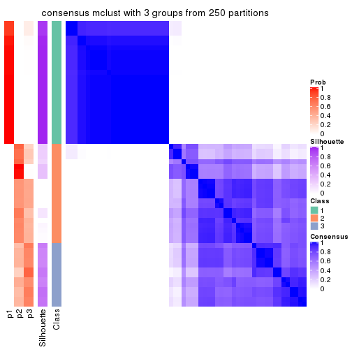
consensus_heatmap(res, k = 4)
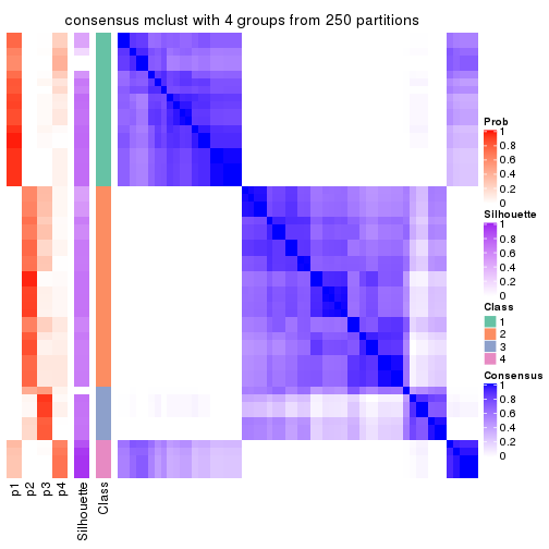
consensus_heatmap(res, k = 5)
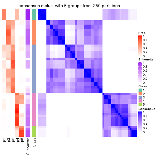
consensus_heatmap(res, k = 6)
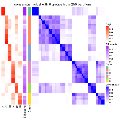
Heatmaps for the membership of samples in all partitions to see how consistent they are:
membership_heatmap(res, k = 2)

membership_heatmap(res, k = 3)
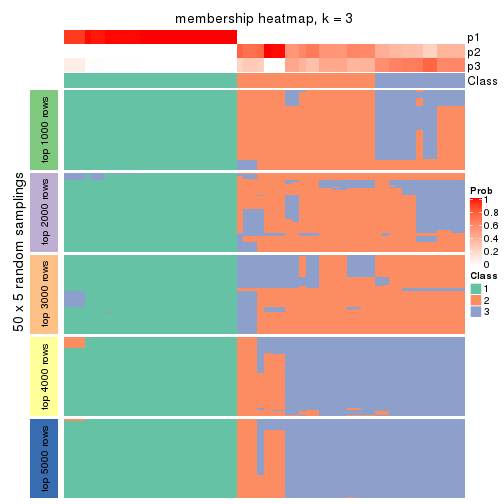
membership_heatmap(res, k = 4)
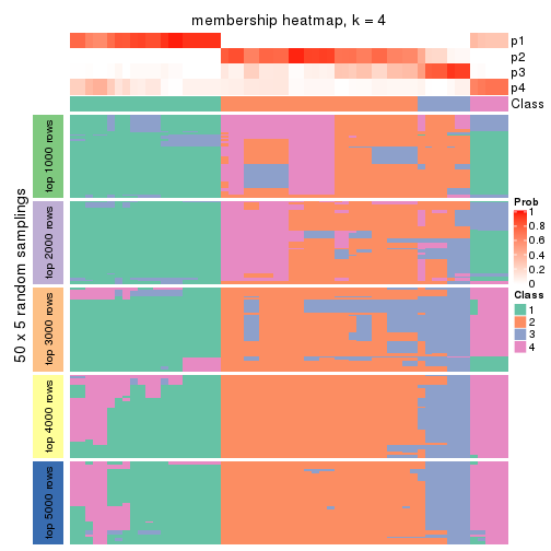
membership_heatmap(res, k = 5)
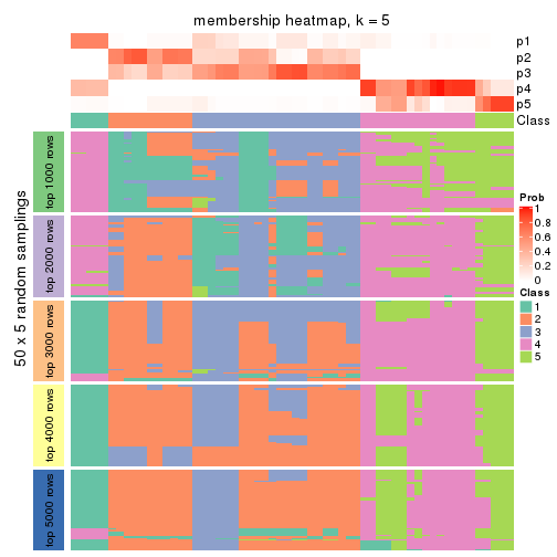
membership_heatmap(res, k = 6)
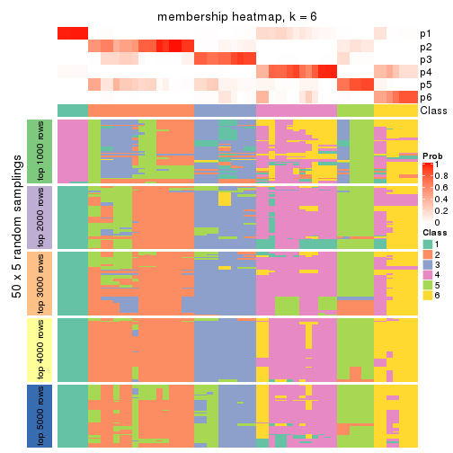
As soon as we have had the classes for columns, we can look for signatures which are significantly different between classes which can be candidate marks for certain classes. Following are the heatmaps for signatures.
Signature heatmaps where rows are scaled:
get_signatures(res, k = 2)

get_signatures(res, k = 3)
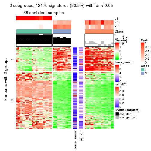
get_signatures(res, k = 4)
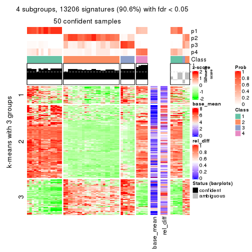
get_signatures(res, k = 5)
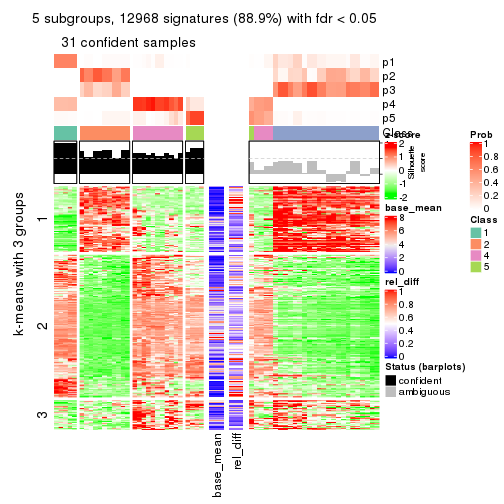
get_signatures(res, k = 6)
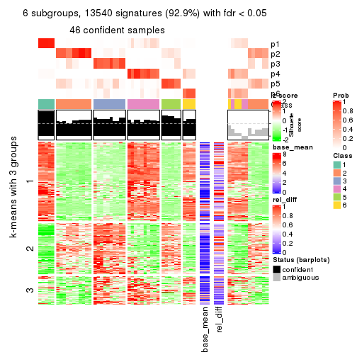
Signature heatmaps where rows are not scaled:
get_signatures(res, k = 2, scale_rows = FALSE)

get_signatures(res, k = 3, scale_rows = FALSE)
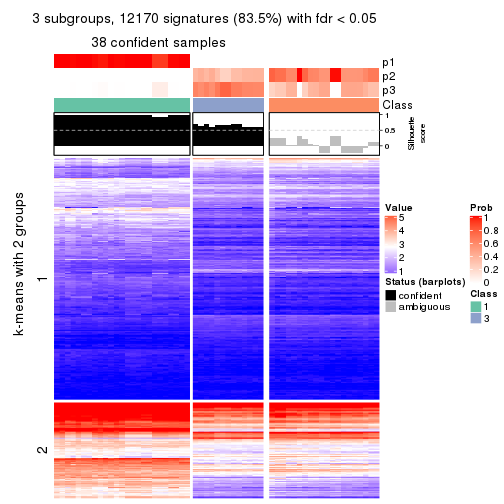
get_signatures(res, k = 4, scale_rows = FALSE)
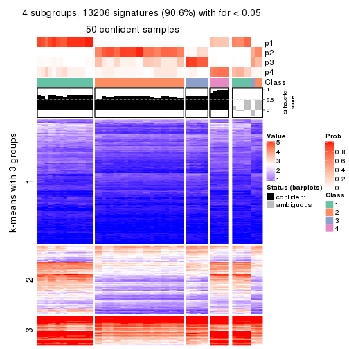
get_signatures(res, k = 5, scale_rows = FALSE)
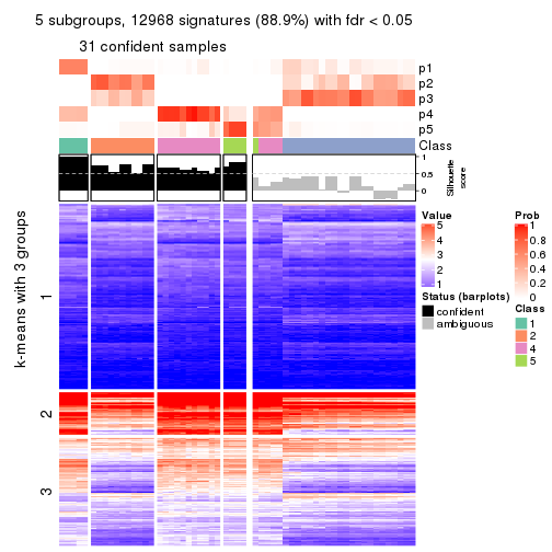
get_signatures(res, k = 6, scale_rows = FALSE)
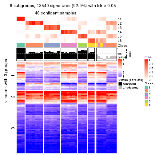
Compare the overlap of signatures from different k:
compare_signatures(res)
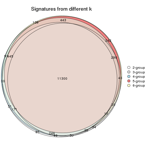
get_signature() returns a data frame invisibly. TO get the list of signatures, the function
call should be assigned to a variable explicitly. In following code, if plot argument is set
to FALSE, no heatmap is plotted while only the differential analysis is performed.
# code only for demonstration
tb = get_signature(res, k = ..., plot = FALSE)
An example of the output of tb is:
#>   which_row         fdr    mean_1    mean_2 scaled_mean_1 scaled_mean_2 km
#> 1        38 0.042760348  8.373488  9.131774    -0.5533452     0.5164555  1
#> 2        40 0.018707592  7.106213  8.469186    -0.6173731     0.5762149  1
#> 3        55 0.019134737 10.221463 11.207825    -0.6159697     0.5749050  1
#> 4        59 0.006059896  5.921854  7.869574    -0.6899429     0.6439467  1
#> 5        60 0.018055526  8.928898 10.211722    -0.6204761     0.5791110  1
#> 6        98 0.009384629 15.714769 14.887706     0.6635654    -0.6193277  2
...
The columns in tb are:
which_row: row indices corresponding to the input matrix.fdr: FDR for the differential test. mean_x: The mean value in group x.scaled_mean_x: The mean value in group x after rows are scaled.km: Row groups if k-means clustering is applied to rows.UMAP plot which shows how samples are separated.
dimension_reduction(res, k = 2, method = "UMAP")

dimension_reduction(res, k = 3, method = "UMAP")
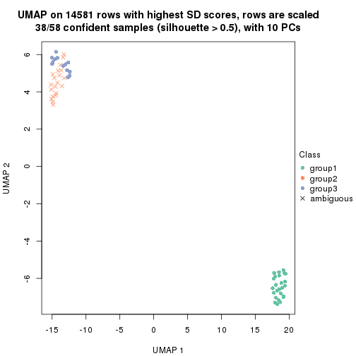
dimension_reduction(res, k = 4, method = "UMAP")
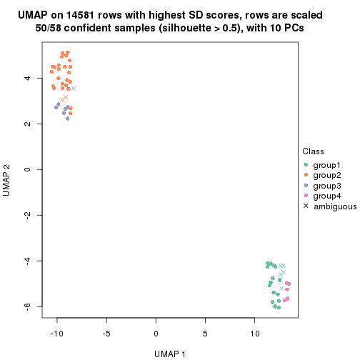
dimension_reduction(res, k = 5, method = "UMAP")
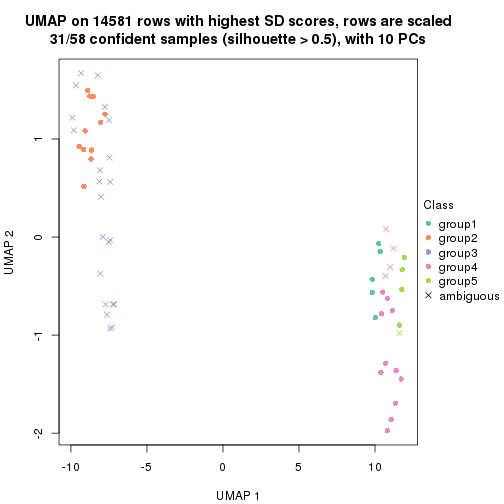
dimension_reduction(res, k = 6, method = "UMAP")
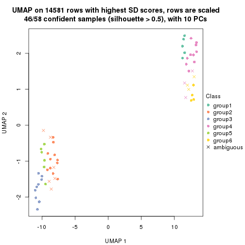
Following heatmap shows how subgroups are split when increasing k:
collect_classes(res)
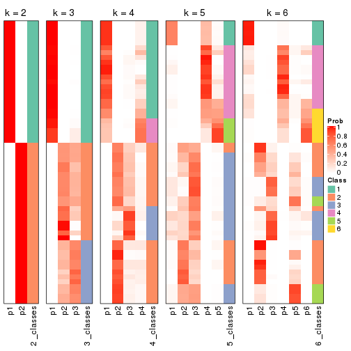
If matrix rows can be associated to genes, consider to use functional_enrichment(res,
...) to perform function enrichment for the signature genes. See this vignette for more detailed explanations.
The object with results only for a single top-value method and a single partition method can be extracted as:
res = res_list["SD", "NMF"]
# you can also extract it by
# res = res_list["SD:NMF"]
A summary of res and all the functions that can be applied to it:
res
#> A 'ConsensusPartition' object with k = 2, 3, 4, 5, 6.
#>   On a matrix with 14581 rows and 58 columns.
#>   Top rows (1000, 2000, 3000, 4000, 5000) are extracted by 'SD' method.
#>   Subgroups are detected by 'NMF' method.
#>   Performed in total 1250 partitions by row resampling.
#>   Best k for subgroups seems to be 3.
#>
#> Following methods can be applied to this 'ConsensusPartition' object:
#>  [1] "cola_report"             "collect_classes"         "collect_plots"
#>  [4] "collect_stats"           "colnames"                "compare_signatures"
#>  [7] "consensus_heatmap"       "dimension_reduction"     "functional_enrichment"
#> [10] "get_anno_col"            "get_anno"                "get_classes"
#> [13] "get_consensus"           "get_matrix"              "get_membership"
#> [16] "get_param"               "get_signatures"          "get_stats"
#> [19] "is_best_k"               "is_stable_k"             "membership_heatmap"
#> [22] "ncol"                    "nrow"                    "plot_ecdf"
#> [25] "rownames"                "select_partition_number" "show"
#> [28] "suggest_best_k"          "test_to_known_factors"
collect_plots() function collects all the plots made from res for all k (number of partitions)
into one single page to provide an easy and fast comparison between different k.
collect_plots(res)
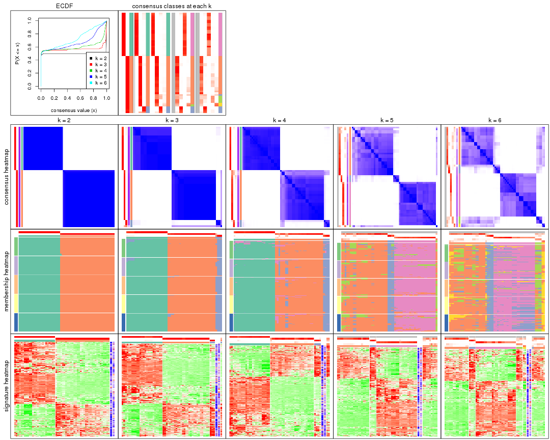
The plots are:
k and the heatmap of
predicted classes for each k.k.k.k.All the plots in panels can be made by individual functions and they are plotted later in this section.
select_partition_number() produces several plots showing different
statistics for choosing “optimized” k. There are following statistics:
k;k, the area increased is defined as \(A_k - A_{k-1}\).The detailed explanations of these statistics can be found in the cola vignette.
Generally speaking, lower PAC score, higher mean silhouette score or higher
concordance corresponds to better partition. Rand index and Jaccard index
measure how similar the current partition is compared to partition with k-1.
If they are too similar, we won't accept k is better than k-1.
select_partition_number(res)
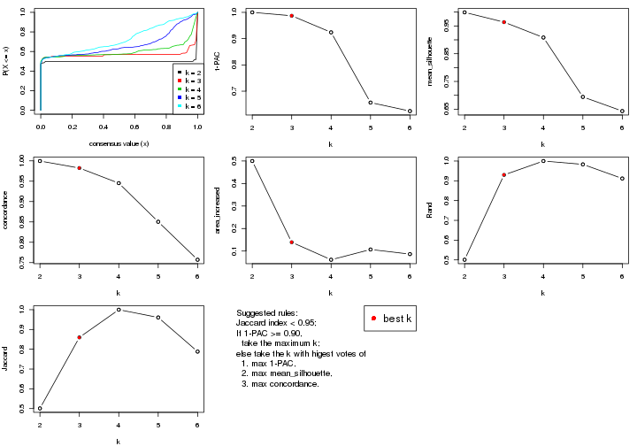
The numeric values for all these statistics can be obtained by get_stats().
get_stats(res)
#>   k 1-PAC mean_silhouette concordance area_increased  Rand Jaccard
#> 2 2 1.000           0.999       1.000         0.4997 0.501   0.501
#> 3 3 0.987           0.964       0.982         0.1391 0.930   0.860
#> 4 4 0.924           0.908       0.945         0.0615 1.000   1.000
#> 5 5 0.657           0.694       0.850         0.1070 0.983   0.961
#> 6 6 0.624           0.643       0.757         0.0865 0.912   0.788
suggest_best_k() suggests the best \(k\) based on these statistics. The rules are as follows:
suggest_best_k(res)
#> [1] 3
#> attr(,"optional")
#> [1] 2
There is also optional best \(k\) = 2 that is worth to check.
Following shows the table of the partitions (You need to click the show/hide
code output link to see it). The membership matrix (columns with name p*)
is inferred by
clue::cl_consensus()
function with the SE method. Basically the value in the membership matrix
represents the probability to belong to a certain group. The finall class
label for an item is determined with the group with highest probability it
belongs to.
In get_classes() function, the entropy is calculated from the membership
matrix and the silhouette score is calculated from the consensus matrix.
cbind(get_classes(res, k = 2), get_membership(res, k = 2))
#>           class entropy silhouette    p1    p2
#> ERR789082     2  0.0000      0.999 0.000 1.000
#> ERR789083     2  0.0000      0.999 0.000 1.000
#> ERR789191     2  0.0000      0.999 0.000 1.000
#> ERR789192     2  0.0000      0.999 0.000 1.000
#> ERR789213     1  0.0000      1.000 1.000 0.000
#> ERR789385     1  0.0000      1.000 1.000 0.000
#> ERR789393     1  0.0000      1.000 1.000 0.000
#> ERR789394     1  0.0000      1.000 1.000 0.000
#> ERR789193     2  0.0000      0.999 0.000 1.000
#> ERR789194     2  0.0376      0.995 0.004 0.996
#> ERR789195     2  0.0000      0.999 0.000 1.000
#> ERR789196     2  0.0000      0.999 0.000 1.000
#> ERR789388     1  0.0000      1.000 1.000 0.000
#> ERR789197     2  0.0000      0.999 0.000 1.000
#> ERR789198     2  0.0000      0.999 0.000 1.000
#> ERR789214     1  0.0000      1.000 1.000 0.000
#> ERR789397     1  0.0000      1.000 1.000 0.000
#> ERR789398     1  0.0000      1.000 1.000 0.000
#> ERR789199     2  0.0000      0.999 0.000 1.000
#> ERR789200     2  0.0000      0.999 0.000 1.000
#> ERR789201     2  0.0000      0.999 0.000 1.000
#> ERR789202     2  0.0000      0.999 0.000 1.000
#> ERR789215     1  0.0000      1.000 1.000 0.000
#> ERR789203     2  0.0000      0.999 0.000 1.000
#> ERR789204     2  0.0000      0.999 0.000 1.000
#> ERR789383     1  0.0000      1.000 1.000 0.000
#> ERR789205     2  0.0000      0.999 0.000 1.000
#> ERR789206     2  0.0000      0.999 0.000 1.000
#> ERR789399     1  0.0000      1.000 1.000 0.000
#> ERR789400     1  0.0000      1.000 1.000 0.000
#> ERR789207     2  0.0000      0.999 0.000 1.000
#> ERR789208     2  0.0000      0.999 0.000 1.000
#> ERR789209     2  0.0000      0.999 0.000 1.000
#> ERR789210     2  0.0000      0.999 0.000 1.000
#> ERR789211     2  0.0000      0.999 0.000 1.000
#> ERR789212     2  0.0000      0.999 0.000 1.000
#> ERR789386     1  0.0000      1.000 1.000 0.000
#> ERR789076     2  0.0000      0.999 0.000 1.000
#> ERR789077     2  0.0000      0.999 0.000 1.000
#> ERR789384     1  0.0000      1.000 1.000 0.000
#> ERR789078     2  0.0000      0.999 0.000 1.000
#> ERR789079     2  0.0000      0.999 0.000 1.000
#> ERR789216     1  0.0000      1.000 1.000 0.000
#> ERR789080     2  0.0000      0.999 0.000 1.000
#> ERR789387     1  0.0000      1.000 1.000 0.000
#> ERR789081     2  0.0000      0.999 0.000 1.000
#> ERR789064     2  0.0000      0.999 0.000 1.000
#> ERR779485     2  0.1633      0.976 0.024 0.976
#> ERR789065     2  0.0000      0.999 0.000 1.000
#> ERR789401     1  0.0000      1.000 1.000 0.000
#> ERR789402     1  0.0000      1.000 1.000 0.000
#> ERR789403     1  0.0000      1.000 1.000 0.000
#> ERR789389     1  0.0000      1.000 1.000 0.000
#> ERR789395     1  0.0000      1.000 1.000 0.000
#> ERR789396     1  0.0000      1.000 1.000 0.000
#> ERR789390     1  0.0000      1.000 1.000 0.000
#> ERR789391     1  0.0000      1.000 1.000 0.000
#> ERR789392     1  0.0000      1.000 1.000 0.000
cbind(get_classes(res, k = 3), get_membership(res, k = 3))
#>           class entropy silhouette    p1    p2    p3
#> ERR789082     2  0.0000      0.994 0.000 1.000 0.000
#> ERR789083     2  0.0000      0.994 0.000 1.000 0.000
#> ERR789191     2  0.0000      0.994 0.000 1.000 0.000
#> ERR789192     2  0.0000      0.994 0.000 1.000 0.000
#> ERR789213     1  0.3116      0.909 0.892 0.000 0.108
#> ERR789385     1  0.2356      0.942 0.928 0.000 0.072
#> ERR789393     1  0.2165      0.945 0.936 0.000 0.064
#> ERR789394     1  0.2165      0.945 0.936 0.000 0.064
#> ERR789193     3  0.0424      0.851 0.000 0.008 0.992
#> ERR789194     3  0.0424      0.851 0.000 0.008 0.992
#> ERR789195     2  0.1860      0.943 0.000 0.948 0.052
#> ERR789196     2  0.1860      0.943 0.000 0.948 0.052
#> ERR789388     1  0.0237      0.983 0.996 0.000 0.004
#> ERR789197     2  0.0000      0.994 0.000 1.000 0.000
#> ERR789198     2  0.0000      0.994 0.000 1.000 0.000
#> ERR789214     1  0.0592      0.981 0.988 0.000 0.012
#> ERR789397     1  0.0424      0.981 0.992 0.000 0.008
#> ERR789398     1  0.0424      0.981 0.992 0.000 0.008
#> ERR789199     2  0.0000      0.994 0.000 1.000 0.000
#> ERR789200     2  0.0000      0.994 0.000 1.000 0.000
#> ERR789201     2  0.0000      0.994 0.000 1.000 0.000
#> ERR789202     2  0.0000      0.994 0.000 1.000 0.000
#> ERR789215     1  0.0237      0.983 0.996 0.000 0.004
#> ERR789203     2  0.0892      0.977 0.000 0.980 0.020
#> ERR789204     2  0.0747      0.981 0.000 0.984 0.016
#> ERR789383     1  0.0237      0.983 0.996 0.000 0.004
#> ERR789205     2  0.0000      0.994 0.000 1.000 0.000
#> ERR789206     2  0.0000      0.994 0.000 1.000 0.000
#> ERR789399     1  0.0000      0.983 1.000 0.000 0.000
#> ERR789400     1  0.0000      0.983 1.000 0.000 0.000
#> ERR789207     2  0.0000      0.994 0.000 1.000 0.000
#> ERR789208     2  0.0000      0.994 0.000 1.000 0.000
#> ERR789209     2  0.0000      0.994 0.000 1.000 0.000
#> ERR789210     2  0.0000      0.994 0.000 1.000 0.000
#> ERR789211     2  0.0000      0.994 0.000 1.000 0.000
#> ERR789212     2  0.0000      0.994 0.000 1.000 0.000
#> ERR789386     1  0.0237      0.983 0.996 0.000 0.004
#> ERR789076     2  0.0237      0.991 0.000 0.996 0.004
#> ERR789077     2  0.0000      0.994 0.000 1.000 0.000
#> ERR789384     1  0.0592      0.981 0.988 0.000 0.012
#> ERR789078     2  0.0000      0.994 0.000 1.000 0.000
#> ERR789079     2  0.0237      0.991 0.000 0.996 0.004
#> ERR789216     1  0.0237      0.983 0.996 0.000 0.004
#> ERR789080     2  0.0237      0.991 0.000 0.996 0.004
#> ERR789387     1  0.0237      0.983 0.996 0.000 0.004
#> ERR789081     2  0.0237      0.991 0.000 0.996 0.004
#> ERR789064     2  0.0000      0.994 0.000 1.000 0.000
#> ERR779485     3  0.0829      0.850 0.004 0.012 0.984
#> ERR789065     3  0.6126      0.334 0.000 0.400 0.600
#> ERR789401     1  0.0000      0.983 1.000 0.000 0.000
#> ERR789402     1  0.0000      0.983 1.000 0.000 0.000
#> ERR789403     1  0.0000      0.983 1.000 0.000 0.000
#> ERR789389     1  0.0237      0.983 0.996 0.000 0.004
#> ERR789395     1  0.0000      0.983 1.000 0.000 0.000
#> ERR789396     1  0.0000      0.983 1.000 0.000 0.000
#> ERR789390     1  0.0000      0.983 1.000 0.000 0.000
#> ERR789391     1  0.0000      0.983 1.000 0.000 0.000
#> ERR789392     1  0.2165      0.945 0.936 0.000 0.064
cbind(get_classes(res, k = 4), get_membership(res, k = 4))
#>           class entropy silhouette    p1    p2    p3    p4
#> ERR789082     2  0.0188      0.921 0.000 0.996 0.000 0.004
#> ERR789083     2  0.0188      0.921 0.000 0.996 0.000 0.004
#> ERR789191     2  0.0336      0.921 0.000 0.992 0.000 0.008
#> ERR789192     2  0.0336      0.921 0.000 0.992 0.000 0.008
#> ERR789213     1  0.3597      0.837 0.836 0.000 0.148 0.016
#> ERR789385     1  0.1888      0.952 0.940 0.000 0.044 0.016
#> ERR789393     1  0.1151      0.973 0.968 0.000 0.008 0.024
#> ERR789394     1  0.1151      0.973 0.968 0.000 0.008 0.024
#> ERR789193     3  0.0469      0.934 0.000 0.000 0.988 0.012
#> ERR789194     3  0.0469      0.934 0.000 0.000 0.988 0.012
#> ERR789195     2  0.1182      0.914 0.000 0.968 0.016 0.016
#> ERR789196     2  0.1182      0.914 0.000 0.968 0.016 0.016
#> ERR789388     1  0.0469      0.980 0.988 0.000 0.000 0.012
#> ERR789197     2  0.0188      0.921 0.000 0.996 0.000 0.004
#> ERR789198     2  0.0188      0.921 0.000 0.996 0.000 0.004
#> ERR789214     1  0.0592      0.979 0.984 0.000 0.000 0.016
#> ERR789397     1  0.0469      0.978 0.988 0.000 0.000 0.012
#> ERR789398     1  0.0469      0.978 0.988 0.000 0.000 0.012
#> ERR789199     2  0.0336      0.921 0.000 0.992 0.000 0.008
#> ERR789200     2  0.0336      0.921 0.000 0.992 0.000 0.008
#> ERR789201     2  0.0188      0.921 0.000 0.996 0.000 0.004
#> ERR789202     2  0.0376      0.921 0.000 0.992 0.004 0.004
#> ERR789215     1  0.0592      0.979 0.984 0.000 0.000 0.016
#> ERR789203     2  0.5957      0.360 0.000 0.588 0.364 0.048
#> ERR789204     2  0.5865      0.421 0.000 0.612 0.340 0.048
#> ERR789383     1  0.0707      0.979 0.980 0.000 0.000 0.020
#> ERR789205     2  0.1767      0.902 0.000 0.944 0.012 0.044
#> ERR789206     2  0.1767      0.902 0.000 0.944 0.012 0.044
#> ERR789399     1  0.0188      0.979 0.996 0.000 0.000 0.004
#> ERR789400     1  0.0188      0.979 0.996 0.000 0.000 0.004
#> ERR789207     2  0.0895      0.918 0.000 0.976 0.004 0.020
#> ERR789208     2  0.0895      0.918 0.000 0.976 0.004 0.020
#> ERR789209     2  0.1706      0.914 0.000 0.948 0.016 0.036
#> ERR789210     2  0.1820      0.912 0.000 0.944 0.020 0.036
#> ERR789211     2  0.1004      0.919 0.000 0.972 0.004 0.024
#> ERR789212     2  0.1151      0.918 0.000 0.968 0.008 0.024
#> ERR789386     1  0.1256      0.975 0.964 0.000 0.008 0.028
#> ERR789076     2  0.6158      0.511 0.000 0.628 0.292 0.080
#> ERR789077     2  0.2198      0.894 0.000 0.920 0.008 0.072
#> ERR789384     1  0.1256      0.976 0.964 0.000 0.008 0.028
#> ERR789078     2  0.2198      0.894 0.000 0.920 0.008 0.072
#> ERR789079     2  0.2011      0.893 0.000 0.920 0.000 0.080
#> ERR789216     1  0.1109      0.976 0.968 0.000 0.004 0.028
#> ERR789080     2  0.4072      0.734 0.000 0.748 0.000 0.252
#> ERR789387     1  0.1211      0.974 0.960 0.000 0.000 0.040
#> ERR789081     2  0.3172      0.833 0.000 0.840 0.000 0.160
#> ERR789064     2  0.0592      0.919 0.000 0.984 0.000 0.016
#> ERR779485     3  0.1722      0.928 0.000 0.008 0.944 0.048
#> ERR789065     3  0.3074      0.808 0.000 0.152 0.848 0.000
#> ERR789401     1  0.0336      0.979 0.992 0.000 0.000 0.008
#> ERR789402     1  0.0469      0.980 0.988 0.000 0.000 0.012
#> ERR789403     1  0.0336      0.979 0.992 0.000 0.000 0.008
#> ERR789389     1  0.1022      0.977 0.968 0.000 0.000 0.032
#> ERR789395     1  0.0469      0.980 0.988 0.000 0.000 0.012
#> ERR789396     1  0.0469      0.980 0.988 0.000 0.000 0.012
#> ERR789390     1  0.0188      0.979 0.996 0.000 0.000 0.004
#> ERR789391     1  0.0188      0.979 0.996 0.000 0.000 0.004
#> ERR789392     1  0.1151      0.973 0.968 0.000 0.008 0.024
cbind(get_classes(res, k = 5), get_membership(res, k = 5))
#>           class entropy silhouette p1    p2    p3    p4    p5
#> ERR789082     2  0.1372     0.7046 NA 0.956 0.024 0.000 0.016
#> ERR789083     2  0.1498     0.7030 NA 0.952 0.024 0.000 0.016
#> ERR789191     2  0.1173     0.7062 NA 0.964 0.012 0.000 0.020
#> ERR789192     2  0.1173     0.7062 NA 0.964 0.012 0.000 0.020
#> ERR789213     4  0.5611     0.7368 NA 0.000 0.148 0.652 0.004
#> ERR789385     4  0.3958     0.8655 NA 0.000 0.040 0.776 0.000
#> ERR789393     4  0.2976     0.8889 NA 0.000 0.012 0.852 0.004
#> ERR789394     4  0.3078     0.8867 NA 0.000 0.016 0.848 0.004
#> ERR789193     3  0.0324     0.8986 NA 0.004 0.992 0.000 0.000
#> ERR789194     3  0.0324     0.8986 NA 0.004 0.992 0.000 0.000
#> ERR789195     2  0.3148     0.6447 NA 0.864 0.072 0.000 0.004
#> ERR789196     2  0.3151     0.6432 NA 0.864 0.068 0.000 0.004
#> ERR789388     4  0.2011     0.9145 NA 0.000 0.000 0.908 0.004
#> ERR789197     2  0.0000     0.7094 NA 1.000 0.000 0.000 0.000
#> ERR789198     2  0.0000     0.7094 NA 1.000 0.000 0.000 0.000
#> ERR789214     4  0.2522     0.9131 NA 0.000 0.000 0.880 0.012
#> ERR789397     4  0.2206     0.9147 NA 0.000 0.004 0.912 0.016
#> ERR789398     4  0.2395     0.9146 NA 0.000 0.008 0.904 0.016
#> ERR789199     2  0.0000     0.7094 NA 1.000 0.000 0.000 0.000
#> ERR789200     2  0.0000     0.7094 NA 1.000 0.000 0.000 0.000
#> ERR789201     2  0.1662     0.7032 NA 0.936 0.004 0.000 0.004
#> ERR789202     2  0.1591     0.7044 NA 0.940 0.004 0.000 0.004
#> ERR789215     4  0.2470     0.9095 NA 0.000 0.000 0.884 0.012
#> ERR789203     2  0.6748    -0.0319 NA 0.440 0.228 0.000 0.004
#> ERR789204     2  0.6714    -0.0184 NA 0.448 0.220 0.000 0.004
#> ERR789383     4  0.2233     0.9125 NA 0.000 0.000 0.904 0.016
#> ERR789205     2  0.4382     0.4612 NA 0.700 0.020 0.000 0.004
#> ERR789206     2  0.4382     0.4612 NA 0.700 0.020 0.000 0.004
#> ERR789399     4  0.1282     0.9119 NA 0.000 0.000 0.952 0.004
#> ERR789400     4  0.1357     0.9124 NA 0.000 0.000 0.948 0.004
#> ERR789207     2  0.2929     0.6662 NA 0.856 0.012 0.000 0.128
#> ERR789208     2  0.2818     0.6674 NA 0.860 0.008 0.000 0.128
#> ERR789209     2  0.4551     0.6319 NA 0.780 0.020 0.000 0.104
#> ERR789210     2  0.4551     0.6319 NA 0.780 0.020 0.000 0.104
#> ERR789211     2  0.3936     0.6521 NA 0.812 0.008 0.000 0.116
#> ERR789212     2  0.3739     0.6574 NA 0.824 0.008 0.000 0.116
#> ERR789386     4  0.2488     0.9082 NA 0.000 0.000 0.872 0.004
#> ERR789076     2  0.6785    -0.3949 NA 0.376 0.340 0.000 0.284
#> ERR789077     2  0.3628     0.5299 NA 0.772 0.012 0.000 0.216
#> ERR789384     4  0.2787     0.9034 NA 0.000 0.004 0.856 0.004
#> ERR789078     2  0.3934     0.4644 NA 0.740 0.016 0.000 0.244
#> ERR789079     2  0.3707     0.3587 NA 0.716 0.000 0.000 0.284
#> ERR789216     4  0.2953     0.9000 NA 0.000 0.000 0.844 0.012
#> ERR789080     5  0.4235     0.0000 NA 0.336 0.000 0.000 0.656
#> ERR789387     4  0.3321     0.8951 NA 0.000 0.000 0.832 0.032
#> ERR789081     2  0.4294    -0.4558 NA 0.532 0.000 0.000 0.468
#> ERR789064     2  0.1341     0.6963 NA 0.944 0.000 0.000 0.056
#> ERR779485     3  0.2249     0.8819 NA 0.008 0.896 0.000 0.000
#> ERR789065     3  0.3670     0.7792 NA 0.112 0.820 0.000 0.000
#> ERR789401     4  0.1043     0.9129 NA 0.000 0.000 0.960 0.000
#> ERR789402     4  0.0880     0.9122 NA 0.000 0.000 0.968 0.000
#> ERR789403     4  0.1043     0.9129 NA 0.000 0.000 0.960 0.000
#> ERR789389     4  0.2286     0.9115 NA 0.000 0.000 0.888 0.004
#> ERR789395     4  0.0880     0.9122 NA 0.000 0.000 0.968 0.000
#> ERR789396     4  0.0880     0.9122 NA 0.000 0.000 0.968 0.000
#> ERR789390     4  0.1282     0.9128 NA 0.000 0.000 0.952 0.004
#> ERR789391     4  0.1282     0.9128 NA 0.000 0.000 0.952 0.004
#> ERR789392     4  0.2976     0.8889 NA 0.000 0.012 0.852 0.004
cbind(get_classes(res, k = 6), get_membership(res, k = 6))
#>           class entropy silhouette p1    p2    p3    p4    p5    p6
#> ERR789082     2  0.2651     0.6526 NA 0.892 0.028 0.000 0.012 0.016
#> ERR789083     2  0.2738     0.6543 NA 0.888 0.028 0.000 0.012 0.020
#> ERR789191     2  0.2678     0.6519 NA 0.888 0.016 0.000 0.016 0.016
#> ERR789192     2  0.2678     0.6519 NA 0.888 0.016 0.000 0.016 0.016
#> ERR789213     4  0.3081     0.6970 NA 0.000 0.072 0.856 0.008 0.004
#> ERR789385     4  0.2635     0.7441 NA 0.000 0.036 0.880 0.004 0.004
#> ERR789393     4  0.3955     0.7815 NA 0.000 0.004 0.648 0.008 0.000
#> ERR789394     4  0.3969     0.7800 NA 0.000 0.004 0.644 0.008 0.000
#> ERR789193     3  0.0260     0.7075 NA 0.000 0.992 0.000 0.000 0.000
#> ERR789194     3  0.0260     0.7075 NA 0.000 0.992 0.000 0.000 0.000
#> ERR789195     2  0.5269     0.2874 NA 0.664 0.192 0.000 0.112 0.000
#> ERR789196     2  0.5389     0.2598 NA 0.652 0.200 0.000 0.112 0.000
#> ERR789388     4  0.1615     0.7758 NA 0.000 0.000 0.928 0.004 0.004
#> ERR789197     2  0.1858     0.6518 NA 0.924 0.012 0.000 0.052 0.000
#> ERR789198     2  0.1858     0.6518 NA 0.924 0.012 0.000 0.052 0.000
#> ERR789214     4  0.1226     0.7697 NA 0.000 0.004 0.952 0.004 0.000
#> ERR789397     4  0.3565     0.7997 NA 0.000 0.004 0.716 0.004 0.000
#> ERR789398     4  0.3586     0.7989 NA 0.000 0.004 0.712 0.004 0.000
#> ERR789199     2  0.0935     0.6648 NA 0.964 0.000 0.000 0.032 0.000
#> ERR789200     2  0.0935     0.6648 NA 0.964 0.000 0.000 0.032 0.000
#> ERR789201     2  0.3956     0.3439 NA 0.716 0.028 0.000 0.252 0.004
#> ERR789202     2  0.4049     0.3252 NA 0.708 0.032 0.000 0.256 0.004
#> ERR789215     4  0.1737     0.7680 NA 0.000 0.000 0.932 0.020 0.008
#> ERR789203     5  0.5703     0.6832 NA 0.220 0.228 0.000 0.548 0.004
#> ERR789204     5  0.5508     0.7089 NA 0.224 0.212 0.000 0.564 0.000
#> ERR789383     4  0.2361     0.7851 NA 0.000 0.000 0.880 0.012 0.004
#> ERR789205     5  0.5087     0.6708 NA 0.412 0.080 0.000 0.508 0.000
#> ERR789206     5  0.5077     0.6865 NA 0.404 0.080 0.000 0.516 0.000
#> ERR789399     4  0.3907     0.7863 NA 0.000 0.000 0.588 0.004 0.000
#> ERR789400     4  0.3907     0.7863 NA 0.000 0.000 0.588 0.004 0.000
#> ERR789207     2  0.4206     0.6154 NA 0.768 0.000 0.000 0.124 0.088
#> ERR789208     2  0.4254     0.6157 NA 0.764 0.000 0.000 0.124 0.092
#> ERR789209     2  0.5689     0.3976 NA 0.588 0.020 0.000 0.300 0.072
#> ERR789210     2  0.5718     0.3814 NA 0.580 0.020 0.000 0.308 0.072
#> ERR789211     2  0.5174     0.5101 NA 0.656 0.008 0.000 0.244 0.072
#> ERR789212     2  0.5046     0.5202 NA 0.664 0.004 0.000 0.240 0.072
#> ERR789386     4  0.0146     0.7632 NA 0.000 0.000 0.996 0.004 0.000
#> ERR789076     3  0.7024    -0.2649 NA 0.312 0.384 0.000 0.056 0.244
#> ERR789077     2  0.3078     0.5457 NA 0.796 0.000 0.000 0.012 0.192
#> ERR789384     4  0.0748     0.7592 NA 0.000 0.016 0.976 0.004 0.000
#> ERR789078     2  0.3171     0.5290 NA 0.784 0.000 0.000 0.012 0.204
#> ERR789079     2  0.3695     0.0311 NA 0.624 0.000 0.000 0.000 0.376
#> ERR789216     4  0.0582     0.7593 NA 0.000 0.004 0.984 0.004 0.004
#> ERR789080     6  0.3050     0.7830 NA 0.236 0.000 0.000 0.000 0.764
#> ERR789387     4  0.1312     0.7513 NA 0.000 0.004 0.956 0.008 0.012
#> ERR789081     6  0.3620     0.7819 NA 0.352 0.000 0.000 0.000 0.648
#> ERR789064     2  0.1349     0.6746 NA 0.940 0.000 0.000 0.004 0.056
#> ERR779485     3  0.2013     0.6822 NA 0.008 0.908 0.000 0.076 0.000
#> ERR789065     3  0.3856     0.5616 NA 0.128 0.788 0.000 0.076 0.004
#> ERR789401     4  0.3923     0.7840 NA 0.000 0.000 0.580 0.004 0.000
#> ERR789402     4  0.3961     0.7746 NA 0.000 0.000 0.556 0.004 0.000
#> ERR789403     4  0.3923     0.7840 NA 0.000 0.000 0.580 0.004 0.000
#> ERR789389     4  0.0632     0.7705 NA 0.000 0.000 0.976 0.000 0.000
#> ERR789395     4  0.3961     0.7746 NA 0.000 0.000 0.556 0.004 0.000
#> ERR789396     4  0.3955     0.7760 NA 0.000 0.000 0.560 0.004 0.000
#> ERR789390     4  0.3944     0.7813 NA 0.000 0.000 0.568 0.004 0.000
#> ERR789391     4  0.3937     0.7827 NA 0.000 0.000 0.572 0.004 0.000
#> ERR789392     4  0.3983     0.7800 NA 0.000 0.004 0.640 0.008 0.000
Heatmaps for the consensus matrix. It visualizes the probability of two samples to be in a same group.
consensus_heatmap(res, k = 2)

consensus_heatmap(res, k = 3)
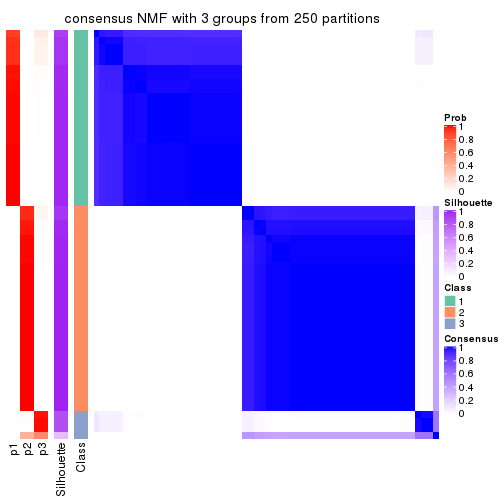
consensus_heatmap(res, k = 4)
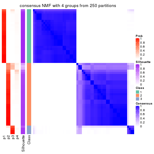
consensus_heatmap(res, k = 5)
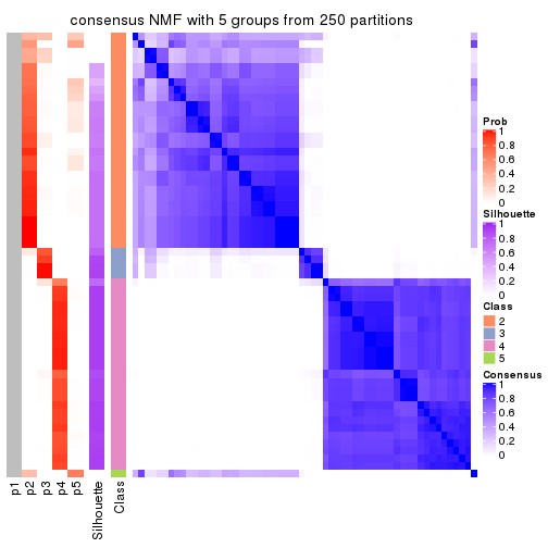
consensus_heatmap(res, k = 6)
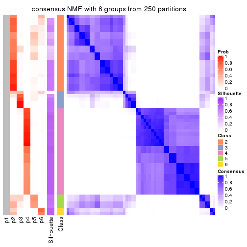
Heatmaps for the membership of samples in all partitions to see how consistent they are:
membership_heatmap(res, k = 2)

membership_heatmap(res, k = 3)
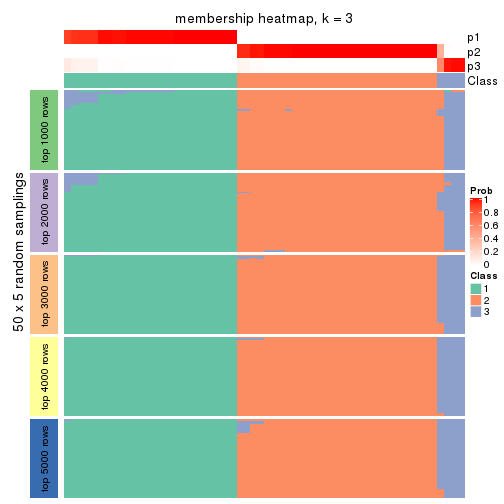
membership_heatmap(res, k = 4)
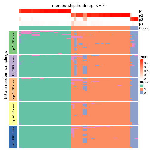
membership_heatmap(res, k = 5)
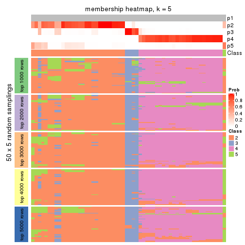
membership_heatmap(res, k = 6)
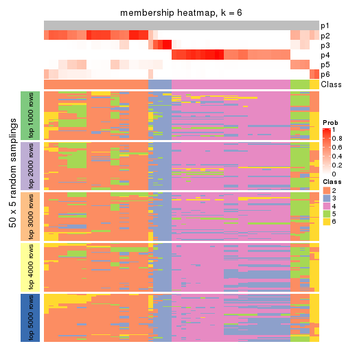
As soon as we have had the classes for columns, we can look for signatures which are significantly different between classes which can be candidate marks for certain classes. Following are the heatmaps for signatures.
Signature heatmaps where rows are scaled:
get_signatures(res, k = 2)

get_signatures(res, k = 3)
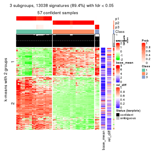
get_signatures(res, k = 4)
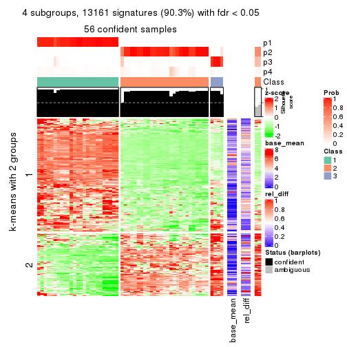
get_signatures(res, k = 5)
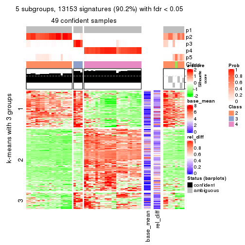
get_signatures(res, k = 6)
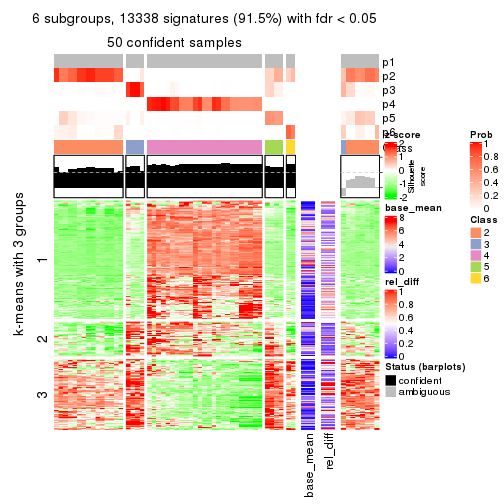
Signature heatmaps where rows are not scaled:
get_signatures(res, k = 2, scale_rows = FALSE)
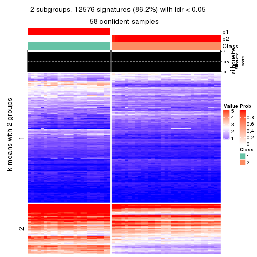
get_signatures(res, k = 3, scale_rows = FALSE)
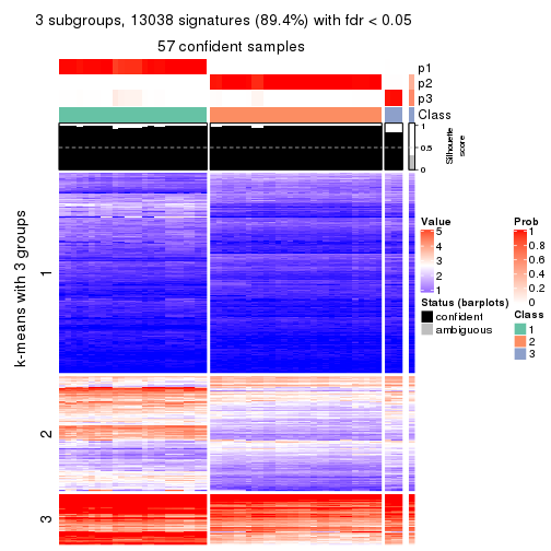
get_signatures(res, k = 4, scale_rows = FALSE)
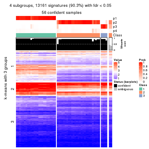
get_signatures(res, k = 5, scale_rows = FALSE)
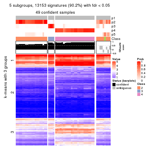
get_signatures(res, k = 6, scale_rows = FALSE)
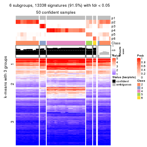
Compare the overlap of signatures from different k:
compare_signatures(res)
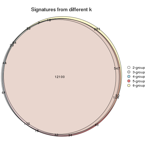
get_signature() returns a data frame invisibly. TO get the list of signatures, the function
call should be assigned to a variable explicitly. In following code, if plot argument is set
to FALSE, no heatmap is plotted while only the differential analysis is performed.
# code only for demonstration
tb = get_signature(res, k = ..., plot = FALSE)
An example of the output of tb is:
#>   which_row         fdr    mean_1    mean_2 scaled_mean_1 scaled_mean_2 km
#> 1        38 0.042760348  8.373488  9.131774    -0.5533452     0.5164555  1
#> 2        40 0.018707592  7.106213  8.469186    -0.6173731     0.5762149  1
#> 3        55 0.019134737 10.221463 11.207825    -0.6159697     0.5749050  1
#> 4        59 0.006059896  5.921854  7.869574    -0.6899429     0.6439467  1
#> 5        60 0.018055526  8.928898 10.211722    -0.6204761     0.5791110  1
#> 6        98 0.009384629 15.714769 14.887706     0.6635654    -0.6193277  2
...
The columns in tb are:
which_row: row indices corresponding to the input matrix.fdr: FDR for the differential test. mean_x: The mean value in group x.scaled_mean_x: The mean value in group x after rows are scaled.km: Row groups if k-means clustering is applied to rows.UMAP plot which shows how samples are separated.
dimension_reduction(res, k = 2, method = "UMAP")

dimension_reduction(res, k = 3, method = "UMAP")

dimension_reduction(res, k = 4, method = "UMAP")
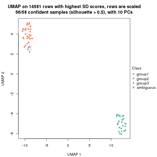
dimension_reduction(res, k = 5, method = "UMAP")
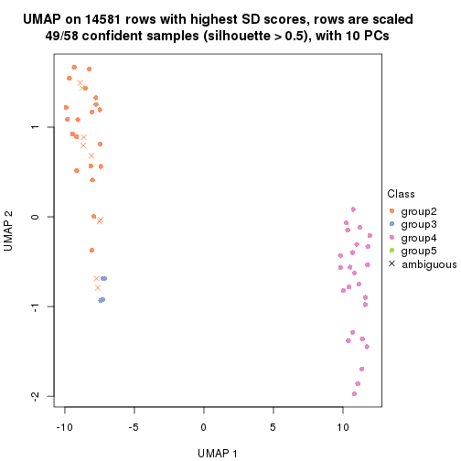
dimension_reduction(res, k = 6, method = "UMAP")
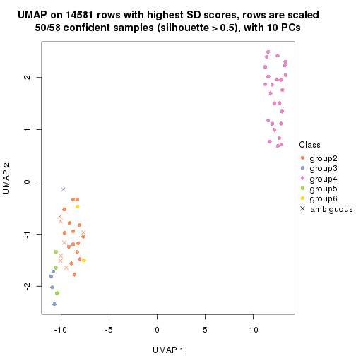
Following heatmap shows how subgroups are split when increasing k:
collect_classes(res)
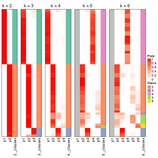
If matrix rows can be associated to genes, consider to use functional_enrichment(res,
...) to perform function enrichment for the signature genes. See this vignette for more detailed explanations.
The object with results only for a single top-value method and a single partition method can be extracted as:
res = res_list["CV", "hclust"]
# you can also extract it by
# res = res_list["CV:hclust"]
A summary of res and all the functions that can be applied to it:
res
#> A 'ConsensusPartition' object with k = 2, 3, 4, 5, 6.
#>   On a matrix with 14581 rows and 58 columns.
#>   Top rows (1000, 2000, 3000, 4000, 5000) are extracted by 'CV' method.
#>   Subgroups are detected by 'hclust' method.
#>   Performed in total 1250 partitions by row resampling.
#>   Best k for subgroups seems to be 3.
#>
#> Following methods can be applied to this 'ConsensusPartition' object:
#>  [1] "cola_report"             "collect_classes"         "collect_plots"
#>  [4] "collect_stats"           "colnames"                "compare_signatures"
#>  [7] "consensus_heatmap"       "dimension_reduction"     "functional_enrichment"
#> [10] "get_anno_col"            "get_anno"                "get_classes"
#> [13] "get_consensus"           "get_matrix"              "get_membership"
#> [16] "get_param"               "get_signatures"          "get_stats"
#> [19] "is_best_k"               "is_stable_k"             "membership_heatmap"
#> [22] "ncol"                    "nrow"                    "plot_ecdf"
#> [25] "rownames"                "select_partition_number" "show"
#> [28] "suggest_best_k"          "test_to_known_factors"
collect_plots() function collects all the plots made from res for all k (number of partitions)
into one single page to provide an easy and fast comparison between different k.
collect_plots(res)
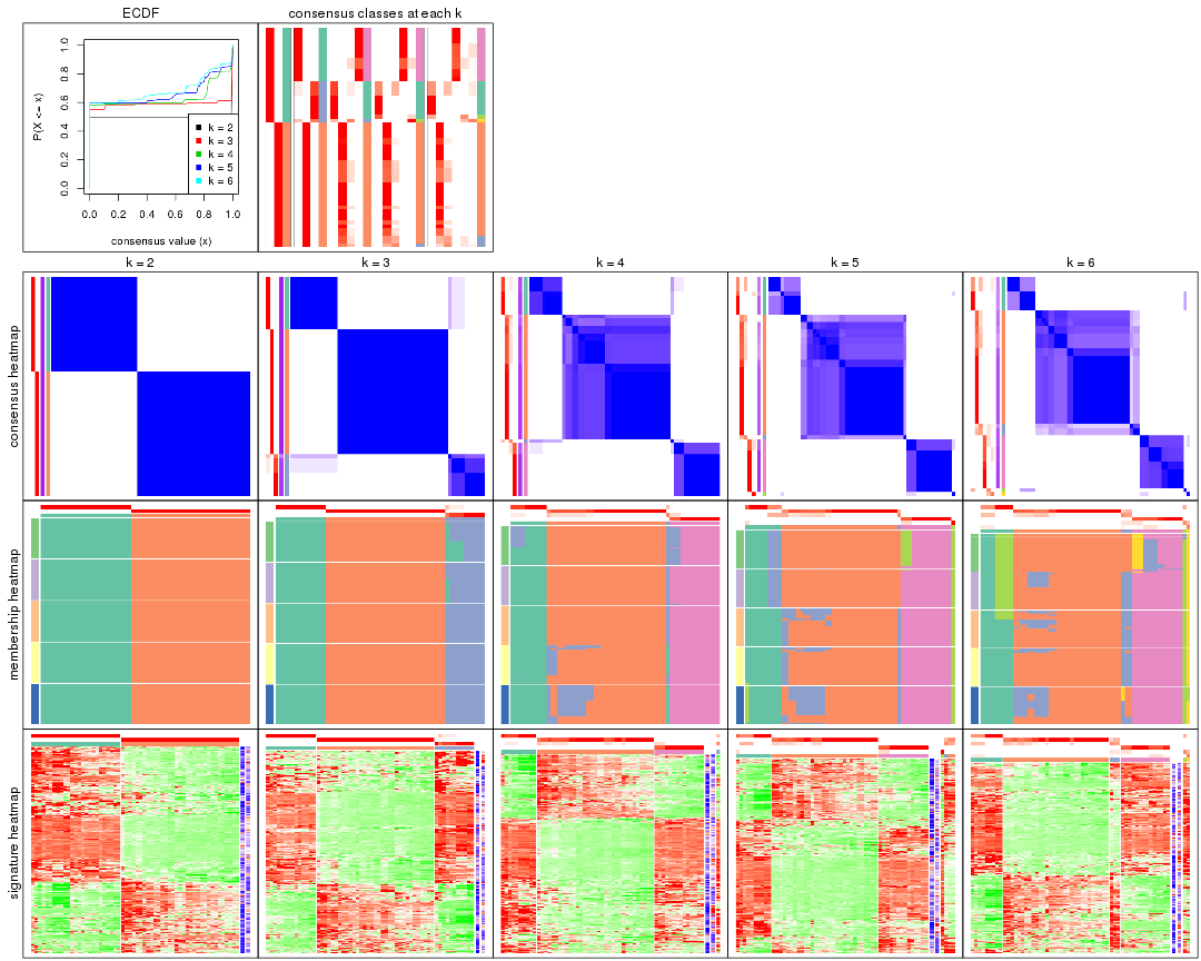
The plots are:
k and the heatmap of
predicted classes for each k.k.k.k.All the plots in panels can be made by individual functions and they are plotted later in this section.
select_partition_number() produces several plots showing different
statistics for choosing “optimized” k. There are following statistics:
k;k, the area increased is defined as \(A_k - A_{k-1}\).The detailed explanations of these statistics can be found in the cola vignette.
Generally speaking, lower PAC score, higher mean silhouette score or higher
concordance corresponds to better partition. Rand index and Jaccard index
measure how similar the current partition is compared to partition with k-1.
If they are too similar, we won't accept k is better than k-1.
select_partition_number(res)

The numeric values for all these statistics can be obtained by get_stats().
get_stats(res)
#>   k 1-PAC mean_silhouette concordance area_increased  Rand Jaccard
#> 2 2 1.000           1.000       1.000         0.4996 0.501   0.501
#> 3 3 0.950           0.979       0.987         0.1803 0.907   0.814
#> 4 4 0.811           0.885       0.936         0.0767 0.994   0.985
#> 5 5 0.803           0.701       0.898         0.0468 0.981   0.952
#> 6 6 0.742           0.749       0.871         0.0341 0.957   0.888
suggest_best_k() suggests the best \(k\) based on these statistics. The rules are as follows:
suggest_best_k(res)
#> [1] 3
#> attr(,"optional")
#> [1] 2
There is also optional best \(k\) = 2 that is worth to check.
Following shows the table of the partitions (You need to click the show/hide
code output link to see it). The membership matrix (columns with name p*)
is inferred by
clue::cl_consensus()
function with the SE method. Basically the value in the membership matrix
represents the probability to belong to a certain group. The finall class
label for an item is determined with the group with highest probability it
belongs to.
In get_classes() function, the entropy is calculated from the membership
matrix and the silhouette score is calculated from the consensus matrix.
cbind(get_classes(res, k = 2), get_membership(res, k = 2))
#>           class entropy silhouette p1 p2
#> ERR789082     2       0          1  0  1
#> ERR789083     2       0          1  0  1
#> ERR789191     2       0          1  0  1
#> ERR789192     2       0          1  0  1
#> ERR789213     1       0          1  1  0
#> ERR789385     1       0          1  1  0
#> ERR789393     1       0          1  1  0
#> ERR789394     1       0          1  1  0
#> ERR789193     2       0          1  0  1
#> ERR789194     2       0          1  0  1
#> ERR789195     2       0          1  0  1
#> ERR789196     2       0          1  0  1
#> ERR789388     1       0          1  1  0
#> ERR789197     2       0          1  0  1
#> ERR789198     2       0          1  0  1
#> ERR789214     1       0          1  1  0
#> ERR789397     1       0          1  1  0
#> ERR789398     1       0          1  1  0
#> ERR789199     2       0          1  0  1
#> ERR789200     2       0          1  0  1
#> ERR789201     2       0          1  0  1
#> ERR789202     2       0          1  0  1
#> ERR789215     1       0          1  1  0
#> ERR789203     2       0          1  0  1
#> ERR789204     2       0          1  0  1
#> ERR789383     1       0          1  1  0
#> ERR789205     2       0          1  0  1
#> ERR789206     2       0          1  0  1
#> ERR789399     1       0          1  1  0
#> ERR789400     1       0          1  1  0
#> ERR789207     2       0          1  0  1
#> ERR789208     2       0          1  0  1
#> ERR789209     2       0          1  0  1
#> ERR789210     2       0          1  0  1
#> ERR789211     2       0          1  0  1
#> ERR789212     2       0          1  0  1
#> ERR789386     1       0          1  1  0
#> ERR789076     2       0          1  0  1
#> ERR789077     2       0          1  0  1
#> ERR789384     1       0          1  1  0
#> ERR789078     2       0          1  0  1
#> ERR789079     2       0          1  0  1
#> ERR789216     1       0          1  1  0
#> ERR789080     2       0          1  0  1
#> ERR789387     1       0          1  1  0
#> ERR789081     2       0          1  0  1
#> ERR789064     2       0          1  0  1
#> ERR779485     2       0          1  0  1
#> ERR789065     2       0          1  0  1
#> ERR789401     1       0          1  1  0
#> ERR789402     1       0          1  1  0
#> ERR789403     1       0          1  1  0
#> ERR789389     1       0          1  1  0
#> ERR789395     1       0          1  1  0
#> ERR789396     1       0          1  1  0
#> ERR789390     1       0          1  1  0
#> ERR789391     1       0          1  1  0
#> ERR789392     1       0          1  1  0
cbind(get_classes(res, k = 3), get_membership(res, k = 3))
#>           class entropy silhouette    p1 p2    p3
#> ERR789082     2   0.000      1.000 0.000  1 0.000
#> ERR789083     2   0.000      1.000 0.000  1 0.000
#> ERR789191     2   0.000      1.000 0.000  1 0.000
#> ERR789192     2   0.000      1.000 0.000  1 0.000
#> ERR789213     1   0.000      1.000 1.000  0 0.000
#> ERR789385     1   0.000      1.000 1.000  0 0.000
#> ERR789393     1   0.000      1.000 1.000  0 0.000
#> ERR789394     1   0.000      1.000 1.000  0 0.000
#> ERR789193     2   0.000      1.000 0.000  1 0.000
#> ERR789194     2   0.000      1.000 0.000  1 0.000
#> ERR789195     2   0.000      1.000 0.000  1 0.000
#> ERR789196     2   0.000      1.000 0.000  1 0.000
#> ERR789388     1   0.000      1.000 1.000  0 0.000
#> ERR789197     2   0.000      1.000 0.000  1 0.000
#> ERR789198     2   0.000      1.000 0.000  1 0.000
#> ERR789214     1   0.000      1.000 1.000  0 0.000
#> ERR789397     1   0.000      1.000 1.000  0 0.000
#> ERR789398     1   0.000      1.000 1.000  0 0.000
#> ERR789199     2   0.000      1.000 0.000  1 0.000
#> ERR789200     2   0.000      1.000 0.000  1 0.000
#> ERR789201     2   0.000      1.000 0.000  1 0.000
#> ERR789202     2   0.000      1.000 0.000  1 0.000
#> ERR789215     3   0.304      0.905 0.104  0 0.896
#> ERR789203     2   0.000      1.000 0.000  1 0.000
#> ERR789204     2   0.000      1.000 0.000  1 0.000
#> ERR789383     3   0.304      0.905 0.104  0 0.896
#> ERR789205     2   0.000      1.000 0.000  1 0.000
#> ERR789206     2   0.000      1.000 0.000  1 0.000
#> ERR789399     3   0.304      0.905 0.104  0 0.896
#> ERR789400     3   0.304      0.905 0.104  0 0.896
#> ERR789207     2   0.000      1.000 0.000  1 0.000
#> ERR789208     2   0.000      1.000 0.000  1 0.000
#> ERR789209     2   0.000      1.000 0.000  1 0.000
#> ERR789210     2   0.000      1.000 0.000  1 0.000
#> ERR789211     2   0.000      1.000 0.000  1 0.000
#> ERR789212     2   0.000      1.000 0.000  1 0.000
#> ERR789386     1   0.000      1.000 1.000  0 0.000
#> ERR789076     2   0.000      1.000 0.000  1 0.000
#> ERR789077     2   0.000      1.000 0.000  1 0.000
#> ERR789384     1   0.000      1.000 1.000  0 0.000
#> ERR789078     2   0.000      1.000 0.000  1 0.000
#> ERR789079     2   0.000      1.000 0.000  1 0.000
#> ERR789216     1   0.000      1.000 1.000  0 0.000
#> ERR789080     2   0.000      1.000 0.000  1 0.000
#> ERR789387     3   0.000      0.926 0.000  0 1.000
#> ERR789081     2   0.000      1.000 0.000  1 0.000
#> ERR789064     2   0.000      1.000 0.000  1 0.000
#> ERR779485     2   0.000      1.000 0.000  1 0.000
#> ERR789065     2   0.000      1.000 0.000  1 0.000
#> ERR789401     3   0.000      0.926 0.000  0 1.000
#> ERR789402     3   0.000      0.926 0.000  0 1.000
#> ERR789403     3   0.000      0.926 0.000  0 1.000
#> ERR789389     3   0.568      0.619 0.316  0 0.684
#> ERR789395     3   0.000      0.926 0.000  0 1.000
#> ERR789396     3   0.000      0.926 0.000  0 1.000
#> ERR789390     1   0.000      1.000 1.000  0 0.000
#> ERR789391     1   0.000      1.000 1.000  0 0.000
#> ERR789392     1   0.000      1.000 1.000  0 0.000
cbind(get_classes(res, k = 4), get_membership(res, k = 4))
#>           class entropy silhouette    p1    p2    p3    p4
#> ERR789082     2  0.0000      0.930 0.000 1.000 0.000 0.000
#> ERR789083     2  0.0000      0.930 0.000 1.000 0.000 0.000
#> ERR789191     2  0.0000      0.930 0.000 1.000 0.000 0.000
#> ERR789192     2  0.0000      0.930 0.000 1.000 0.000 0.000
#> ERR789213     4  0.0000      0.954 0.000 0.000 0.000 1.000
#> ERR789385     4  0.0000      0.954 0.000 0.000 0.000 1.000
#> ERR789393     4  0.0000      0.954 0.000 0.000 0.000 1.000
#> ERR789394     4  0.0000      0.954 0.000 0.000 0.000 1.000
#> ERR789193     2  0.3444      0.794 0.000 0.816 0.184 0.000
#> ERR789194     2  0.3444      0.794 0.000 0.816 0.184 0.000
#> ERR789195     2  0.0469      0.927 0.000 0.988 0.012 0.000
#> ERR789196     2  0.0469      0.927 0.000 0.988 0.012 0.000
#> ERR789388     4  0.0000      0.954 0.000 0.000 0.000 1.000
#> ERR789197     2  0.0000      0.930 0.000 1.000 0.000 0.000
#> ERR789198     2  0.0000      0.930 0.000 1.000 0.000 0.000
#> ERR789214     4  0.0000      0.954 0.000 0.000 0.000 1.000
#> ERR789397     4  0.0000      0.954 0.000 0.000 0.000 1.000
#> ERR789398     4  0.0000      0.954 0.000 0.000 0.000 1.000
#> ERR789199     2  0.0000      0.930 0.000 1.000 0.000 0.000
#> ERR789200     2  0.0000      0.930 0.000 1.000 0.000 0.000
#> ERR789201     2  0.3400      0.858 0.000 0.820 0.180 0.000
#> ERR789202     2  0.3400      0.858 0.000 0.820 0.180 0.000
#> ERR789215     1  0.2469      0.852 0.892 0.000 0.108 0.000
#> ERR789203     2  0.3400      0.858 0.000 0.820 0.180 0.000
#> ERR789204     2  0.3400      0.858 0.000 0.820 0.180 0.000
#> ERR789383     1  0.2469      0.852 0.892 0.000 0.108 0.000
#> ERR789205     2  0.3400      0.858 0.000 0.820 0.180 0.000
#> ERR789206     2  0.3400      0.858 0.000 0.820 0.180 0.000
#> ERR789399     1  0.2469      0.852 0.892 0.000 0.108 0.000
#> ERR789400     1  0.2469      0.852 0.892 0.000 0.108 0.000
#> ERR789207     2  0.0000      0.930 0.000 1.000 0.000 0.000
#> ERR789208     2  0.0000      0.930 0.000 1.000 0.000 0.000
#> ERR789209     2  0.0000      0.930 0.000 1.000 0.000 0.000
#> ERR789210     2  0.0000      0.930 0.000 1.000 0.000 0.000
#> ERR789211     2  0.0000      0.930 0.000 1.000 0.000 0.000
#> ERR789212     2  0.0000      0.930 0.000 1.000 0.000 0.000
#> ERR789386     4  0.3528      0.804 0.000 0.000 0.192 0.808
#> ERR789076     2  0.3219      0.864 0.000 0.836 0.164 0.000
#> ERR789077     2  0.0000      0.930 0.000 1.000 0.000 0.000
#> ERR789384     4  0.3528      0.804 0.000 0.000 0.192 0.808
#> ERR789078     2  0.0000      0.930 0.000 1.000 0.000 0.000
#> ERR789079     2  0.0000      0.930 0.000 1.000 0.000 0.000
#> ERR789216     4  0.3528      0.804 0.000 0.000 0.192 0.808
#> ERR789080     2  0.3266      0.862 0.000 0.832 0.168 0.000
#> ERR789387     1  0.0188      0.905 0.996 0.000 0.004 0.000
#> ERR789081     2  0.0000      0.930 0.000 1.000 0.000 0.000
#> ERR789064     2  0.2216      0.901 0.000 0.908 0.092 0.000
#> ERR779485     2  0.4679      0.688 0.000 0.648 0.352 0.000
#> ERR789065     2  0.2216      0.901 0.000 0.908 0.092 0.000
#> ERR789401     1  0.0000      0.908 1.000 0.000 0.000 0.000
#> ERR789402     1  0.0000      0.908 1.000 0.000 0.000 0.000
#> ERR789403     1  0.0000      0.908 1.000 0.000 0.000 0.000
#> ERR789389     3  0.4679      0.000 0.352 0.000 0.648 0.000
#> ERR789395     1  0.0000      0.908 1.000 0.000 0.000 0.000
#> ERR789396     1  0.0000      0.908 1.000 0.000 0.000 0.000
#> ERR789390     4  0.0000      0.954 0.000 0.000 0.000 1.000
#> ERR789391     4  0.0000      0.954 0.000 0.000 0.000 1.000
#> ERR789392     4  0.0000      0.954 0.000 0.000 0.000 1.000
cbind(get_classes(res, k = 5), get_membership(res, k = 5))
#>           class entropy silhouette    p1    p2    p3    p4    p5
#> ERR789082     2   0.000      0.809 0.000 1.000 0.000 0.000 0.000
#> ERR789083     2   0.000      0.809 0.000 1.000 0.000 0.000 0.000
#> ERR789191     2   0.000      0.809 0.000 1.000 0.000 0.000 0.000
#> ERR789192     2   0.000      0.809 0.000 1.000 0.000 0.000 0.000
#> ERR789213     4   0.000      0.953 0.000 0.000 0.000 1.000 0.000
#> ERR789385     4   0.000      0.953 0.000 0.000 0.000 1.000 0.000
#> ERR789393     4   0.000      0.953 0.000 0.000 0.000 1.000 0.000
#> ERR789394     4   0.000      0.953 0.000 0.000 0.000 1.000 0.000
#> ERR789193     2   0.423     -0.510 0.000 0.576 0.424 0.000 0.000
#> ERR789194     2   0.423     -0.510 0.000 0.576 0.424 0.000 0.000
#> ERR789195     2   0.179      0.734 0.000 0.916 0.084 0.000 0.000
#> ERR789196     2   0.179      0.734 0.000 0.916 0.084 0.000 0.000
#> ERR789388     4   0.000      0.953 0.000 0.000 0.000 1.000 0.000
#> ERR789197     2   0.000      0.809 0.000 1.000 0.000 0.000 0.000
#> ERR789198     2   0.000      0.809 0.000 1.000 0.000 0.000 0.000
#> ERR789214     4   0.000      0.953 0.000 0.000 0.000 1.000 0.000
#> ERR789397     4   0.000      0.953 0.000 0.000 0.000 1.000 0.000
#> ERR789398     4   0.000      0.953 0.000 0.000 0.000 1.000 0.000
#> ERR789199     2   0.000      0.809 0.000 1.000 0.000 0.000 0.000
#> ERR789200     2   0.000      0.809 0.000 1.000 0.000 0.000 0.000
#> ERR789201     2   0.331      0.558 0.000 0.776 0.224 0.000 0.000
#> ERR789202     2   0.331      0.558 0.000 0.776 0.224 0.000 0.000
#> ERR789215     1   0.417      0.676 0.604 0.000 0.396 0.000 0.000
#> ERR789203     2   0.351      0.501 0.000 0.748 0.252 0.000 0.000
#> ERR789204     2   0.351      0.501 0.000 0.748 0.252 0.000 0.000
#> ERR789383     1   0.417      0.676 0.604 0.000 0.396 0.000 0.000
#> ERR789205     2   0.351      0.501 0.000 0.748 0.252 0.000 0.000
#> ERR789206     2   0.351      0.501 0.000 0.748 0.252 0.000 0.000
#> ERR789399     1   0.417      0.676 0.604 0.000 0.396 0.000 0.000
#> ERR789400     1   0.417      0.676 0.604 0.000 0.396 0.000 0.000
#> ERR789207     2   0.000      0.809 0.000 1.000 0.000 0.000 0.000
#> ERR789208     2   0.000      0.809 0.000 1.000 0.000 0.000 0.000
#> ERR789209     2   0.000      0.809 0.000 1.000 0.000 0.000 0.000
#> ERR789210     2   0.000      0.809 0.000 1.000 0.000 0.000 0.000
#> ERR789211     2   0.000      0.809 0.000 1.000 0.000 0.000 0.000
#> ERR789212     2   0.000      0.809 0.000 1.000 0.000 0.000 0.000
#> ERR789386     4   0.304      0.799 0.000 0.000 0.000 0.808 0.192
#> ERR789076     2   0.307      0.598 0.000 0.804 0.196 0.000 0.000
#> ERR789077     2   0.000      0.809 0.000 1.000 0.000 0.000 0.000
#> ERR789384     4   0.304      0.799 0.000 0.000 0.000 0.808 0.192
#> ERR789078     2   0.000      0.809 0.000 1.000 0.000 0.000 0.000
#> ERR789079     2   0.000      0.809 0.000 1.000 0.000 0.000 0.000
#> ERR789216     4   0.304      0.799 0.000 0.000 0.000 0.808 0.192
#> ERR789080     2   0.293      0.611 0.000 0.820 0.180 0.000 0.000
#> ERR789387     1   0.318      0.550 0.792 0.000 0.000 0.000 0.208
#> ERR789081     2   0.000      0.809 0.000 1.000 0.000 0.000 0.000
#> ERR789064     2   0.277      0.657 0.000 0.836 0.164 0.000 0.000
#> ERR779485     3   0.417      0.000 0.000 0.396 0.604 0.000 0.000
#> ERR789065     2   0.277      0.657 0.000 0.836 0.164 0.000 0.000
#> ERR789401     1   0.000      0.775 1.000 0.000 0.000 0.000 0.000
#> ERR789402     1   0.000      0.775 1.000 0.000 0.000 0.000 0.000
#> ERR789403     1   0.000      0.775 1.000 0.000 0.000 0.000 0.000
#> ERR789389     5   0.000      0.000 0.000 0.000 0.000 0.000 1.000
#> ERR789395     1   0.000      0.775 1.000 0.000 0.000 0.000 0.000
#> ERR789396     1   0.000      0.775 1.000 0.000 0.000 0.000 0.000
#> ERR789390     4   0.000      0.953 0.000 0.000 0.000 1.000 0.000
#> ERR789391     4   0.000      0.953 0.000 0.000 0.000 1.000 0.000
#> ERR789392     4   0.000      0.953 0.000 0.000 0.000 1.000 0.000
cbind(get_classes(res, k = 6), get_membership(res, k = 6))
#>           class entropy silhouette    p1    p2    p3    p4    p5    p6
#> ERR789082     2  0.0000      0.858 0.000 1.000 0.000 0.000 0.000 0.000
#> ERR789083     2  0.0000      0.858 0.000 1.000 0.000 0.000 0.000 0.000
#> ERR789191     2  0.0000      0.858 0.000 1.000 0.000 0.000 0.000 0.000
#> ERR789192     2  0.0000      0.858 0.000 1.000 0.000 0.000 0.000 0.000
#> ERR789213     4  0.0000      0.908 0.000 0.000 0.000 1.000 0.000 0.000
#> ERR789385     4  0.0000      0.908 0.000 0.000 0.000 1.000 0.000 0.000
#> ERR789393     4  0.0000      0.908 0.000 0.000 0.000 1.000 0.000 0.000
#> ERR789394     4  0.0000      0.908 0.000 0.000 0.000 1.000 0.000 0.000
#> ERR789193     3  0.5555      0.837 0.000 0.380 0.480 0.000 0.140 0.000
#> ERR789194     3  0.5555      0.837 0.000 0.380 0.480 0.000 0.140 0.000
#> ERR789195     2  0.1663      0.794 0.000 0.912 0.088 0.000 0.000 0.000
#> ERR789196     2  0.1663      0.794 0.000 0.912 0.088 0.000 0.000 0.000
#> ERR789388     4  0.2491      0.878 0.000 0.000 0.000 0.836 0.000 0.164
#> ERR789197     2  0.0000      0.858 0.000 1.000 0.000 0.000 0.000 0.000
#> ERR789198     2  0.0000      0.858 0.000 1.000 0.000 0.000 0.000 0.000
#> ERR789214     4  0.2491      0.878 0.000 0.000 0.000 0.836 0.000 0.164
#> ERR789397     4  0.2491      0.878 0.000 0.000 0.000 0.836 0.000 0.164
#> ERR789398     4  0.2491      0.878 0.000 0.000 0.000 0.836 0.000 0.164
#> ERR789199     2  0.0000      0.858 0.000 1.000 0.000 0.000 0.000 0.000
#> ERR789200     2  0.0000      0.858 0.000 1.000 0.000 0.000 0.000 0.000
#> ERR789201     2  0.2969      0.691 0.000 0.776 0.224 0.000 0.000 0.000
#> ERR789202     2  0.2969      0.691 0.000 0.776 0.224 0.000 0.000 0.000
#> ERR789215     1  0.5219      0.611 0.552 0.000 0.340 0.000 0.000 0.108
#> ERR789203     2  0.3531      0.537 0.000 0.672 0.328 0.000 0.000 0.000
#> ERR789204     2  0.3531      0.537 0.000 0.672 0.328 0.000 0.000 0.000
#> ERR789383     1  0.5219      0.611 0.552 0.000 0.340 0.000 0.000 0.108
#> ERR789205     2  0.3531      0.537 0.000 0.672 0.328 0.000 0.000 0.000
#> ERR789206     2  0.3531      0.537 0.000 0.672 0.328 0.000 0.000 0.000
#> ERR789399     1  0.5219      0.611 0.552 0.000 0.340 0.000 0.000 0.108
#> ERR789400     1  0.5219      0.611 0.552 0.000 0.340 0.000 0.000 0.108
#> ERR789207     2  0.0000      0.858 0.000 1.000 0.000 0.000 0.000 0.000
#> ERR789208     2  0.0000      0.858 0.000 1.000 0.000 0.000 0.000 0.000
#> ERR789209     2  0.0000      0.858 0.000 1.000 0.000 0.000 0.000 0.000
#> ERR789210     2  0.0000      0.858 0.000 1.000 0.000 0.000 0.000 0.000
#> ERR789211     2  0.0000      0.858 0.000 1.000 0.000 0.000 0.000 0.000
#> ERR789212     2  0.0000      0.858 0.000 1.000 0.000 0.000 0.000 0.000
#> ERR789386     4  0.3213      0.835 0.000 0.000 0.000 0.808 0.160 0.032
#> ERR789076     2  0.2793      0.712 0.000 0.800 0.200 0.000 0.000 0.000
#> ERR789077     2  0.0000      0.858 0.000 1.000 0.000 0.000 0.000 0.000
#> ERR789384     4  0.3213      0.835 0.000 0.000 0.000 0.808 0.160 0.032
#> ERR789078     2  0.0000      0.858 0.000 1.000 0.000 0.000 0.000 0.000
#> ERR789079     2  0.0000      0.858 0.000 1.000 0.000 0.000 0.000 0.000
#> ERR789216     4  0.3213      0.835 0.000 0.000 0.000 0.808 0.160 0.032
#> ERR789080     2  0.2631      0.722 0.000 0.820 0.180 0.000 0.000 0.000
#> ERR789387     5  0.3789      0.000 0.416 0.000 0.000 0.000 0.584 0.000
#> ERR789081     2  0.0000      0.858 0.000 1.000 0.000 0.000 0.000 0.000
#> ERR789064     2  0.3076      0.649 0.000 0.760 0.240 0.000 0.000 0.000
#> ERR779485     3  0.6133      0.625 0.000 0.200 0.588 0.000 0.140 0.072
#> ERR789065     2  0.3076      0.649 0.000 0.760 0.240 0.000 0.000 0.000
#> ERR789401     1  0.0000      0.611 1.000 0.000 0.000 0.000 0.000 0.000
#> ERR789402     1  0.0000      0.611 1.000 0.000 0.000 0.000 0.000 0.000
#> ERR789403     1  0.0000      0.611 1.000 0.000 0.000 0.000 0.000 0.000
#> ERR789389     6  0.3607      0.000 0.000 0.000 0.000 0.000 0.348 0.652
#> ERR789395     1  0.0000      0.611 1.000 0.000 0.000 0.000 0.000 0.000
#> ERR789396     1  0.0000      0.611 1.000 0.000 0.000 0.000 0.000 0.000
#> ERR789390     4  0.0713      0.908 0.000 0.000 0.000 0.972 0.000 0.028
#> ERR789391     4  0.0713      0.908 0.000 0.000 0.000 0.972 0.000 0.028
#> ERR789392     4  0.0000      0.908 0.000 0.000 0.000 1.000 0.000 0.000
Heatmaps for the consensus matrix. It visualizes the probability of two samples to be in a same group.
consensus_heatmap(res, k = 2)

consensus_heatmap(res, k = 3)
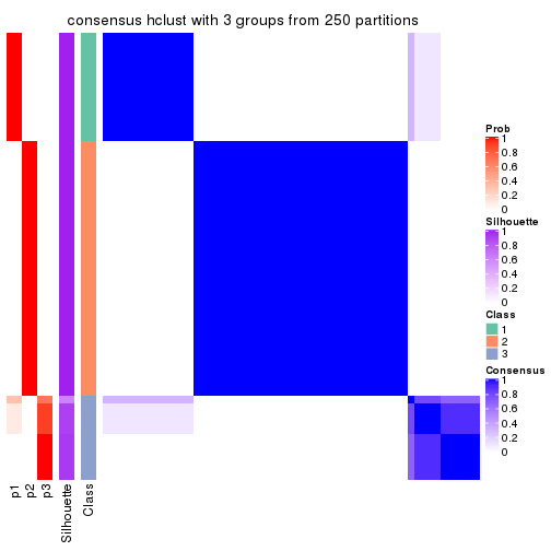
consensus_heatmap(res, k = 4)
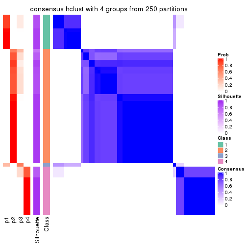
consensus_heatmap(res, k = 5)
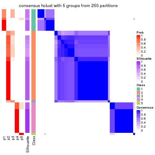
consensus_heatmap(res, k = 6)
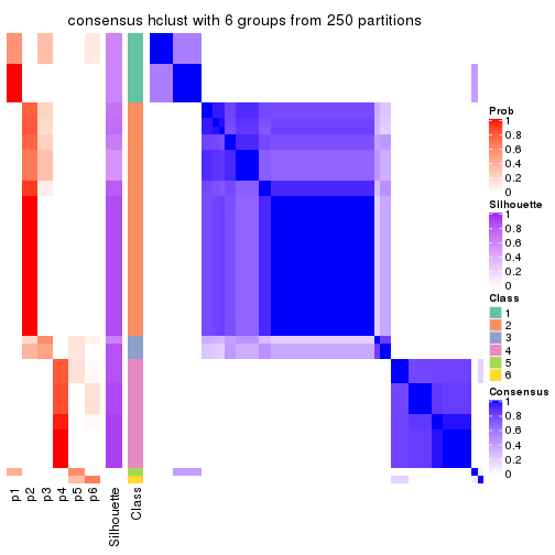
Heatmaps for the membership of samples in all partitions to see how consistent they are:
membership_heatmap(res, k = 2)

membership_heatmap(res, k = 3)
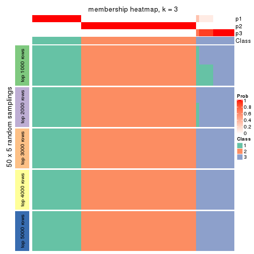
membership_heatmap(res, k = 4)
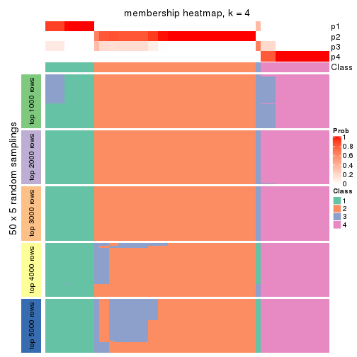
membership_heatmap(res, k = 5)
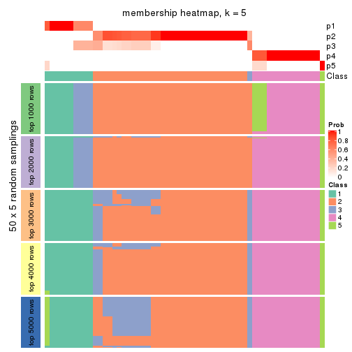
membership_heatmap(res, k = 6)
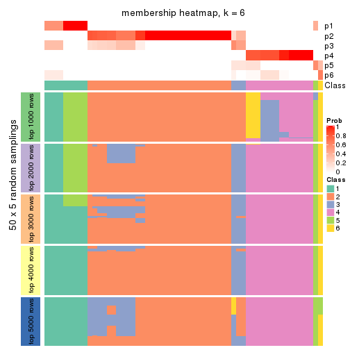
As soon as we have had the classes for columns, we can look for signatures which are significantly different between classes which can be candidate marks for certain classes. Following are the heatmaps for signatures.
Signature heatmaps where rows are scaled:
get_signatures(res, k = 2)

get_signatures(res, k = 3)
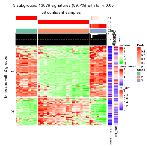
get_signatures(res, k = 4)
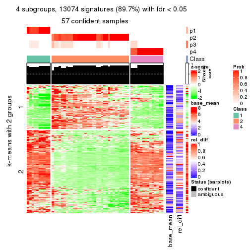
get_signatures(res, k = 5)
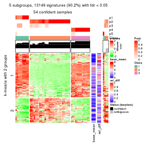
get_signatures(res, k = 6)
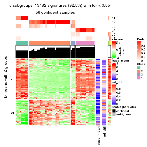
Signature heatmaps where rows are not scaled:
get_signatures(res, k = 2, scale_rows = FALSE)

get_signatures(res, k = 3, scale_rows = FALSE)
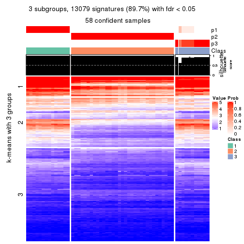
get_signatures(res, k = 4, scale_rows = FALSE)
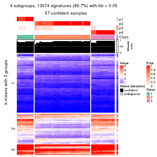
get_signatures(res, k = 5, scale_rows = FALSE)
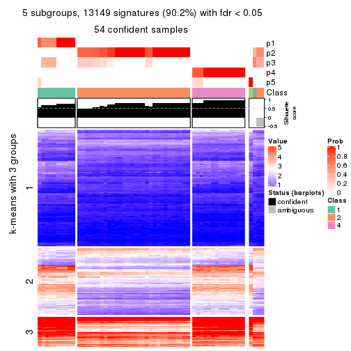
get_signatures(res, k = 6, scale_rows = FALSE)
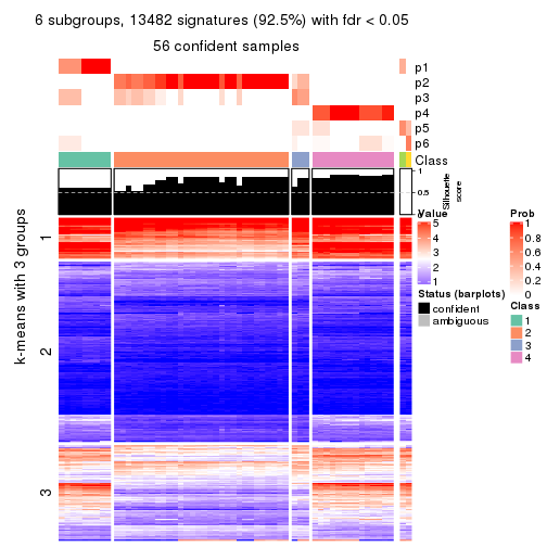
Compare the overlap of signatures from different k:
compare_signatures(res)
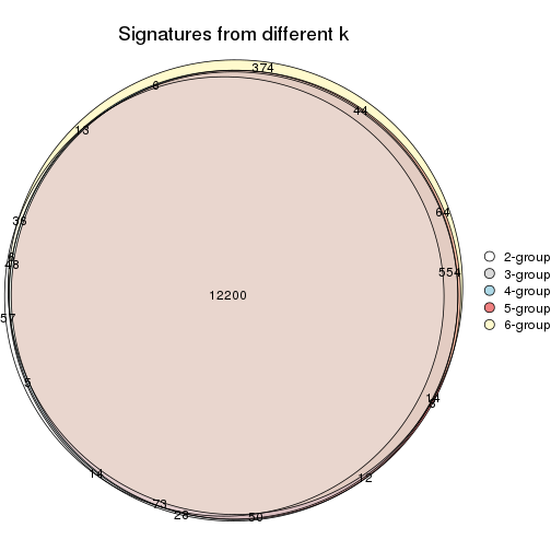
get_signature() returns a data frame invisibly. TO get the list of signatures, the function
call should be assigned to a variable explicitly. In following code, if plot argument is set
to FALSE, no heatmap is plotted while only the differential analysis is performed.
# code only for demonstration
tb = get_signature(res, k = ..., plot = FALSE)
An example of the output of tb is:
#>   which_row         fdr    mean_1    mean_2 scaled_mean_1 scaled_mean_2 km
#> 1        38 0.042760348  8.373488  9.131774    -0.5533452     0.5164555  1
#> 2        40 0.018707592  7.106213  8.469186    -0.6173731     0.5762149  1
#> 3        55 0.019134737 10.221463 11.207825    -0.6159697     0.5749050  1
#> 4        59 0.006059896  5.921854  7.869574    -0.6899429     0.6439467  1
#> 5        60 0.018055526  8.928898 10.211722    -0.6204761     0.5791110  1
#> 6        98 0.009384629 15.714769 14.887706     0.6635654    -0.6193277  2
...
The columns in tb are:
which_row: row indices corresponding to the input matrix.fdr: FDR for the differential test. mean_x: The mean value in group x.scaled_mean_x: The mean value in group x after rows are scaled.km: Row groups if k-means clustering is applied to rows.UMAP plot which shows how samples are separated.
dimension_reduction(res, k = 2, method = "UMAP")

dimension_reduction(res, k = 3, method = "UMAP")

dimension_reduction(res, k = 4, method = "UMAP")

dimension_reduction(res, k = 5, method = "UMAP")
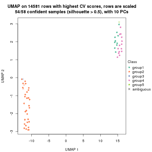
dimension_reduction(res, k = 6, method = "UMAP")
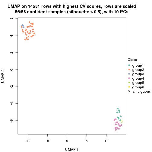
Following heatmap shows how subgroups are split when increasing k:
collect_classes(res)
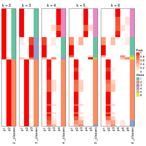
If matrix rows can be associated to genes, consider to use functional_enrichment(res,
...) to perform function enrichment for the signature genes. See this vignette for more detailed explanations.
The object with results only for a single top-value method and a single partition method can be extracted as:
res = res_list["CV", "kmeans"]
# you can also extract it by
# res = res_list["CV:kmeans"]
A summary of res and all the functions that can be applied to it:
res
#> A 'ConsensusPartition' object with k = 2, 3, 4, 5, 6.
#>   On a matrix with 14581 rows and 58 columns.
#>   Top rows (1000, 2000, 3000, 4000, 5000) are extracted by 'CV' method.
#>   Subgroups are detected by 'kmeans' method.
#>   Performed in total 1250 partitions by row resampling.
#>   Best k for subgroups seems to be 2.
#>
#> Following methods can be applied to this 'ConsensusPartition' object:
#>  [1] "cola_report"             "collect_classes"         "collect_plots"
#>  [4] "collect_stats"           "colnames"                "compare_signatures"
#>  [7] "consensus_heatmap"       "dimension_reduction"     "functional_enrichment"
#> [10] "get_anno_col"            "get_anno"                "get_classes"
#> [13] "get_consensus"           "get_matrix"              "get_membership"
#> [16] "get_param"               "get_signatures"          "get_stats"
#> [19] "is_best_k"               "is_stable_k"             "membership_heatmap"
#> [22] "ncol"                    "nrow"                    "plot_ecdf"
#> [25] "rownames"                "select_partition_number" "show"
#> [28] "suggest_best_k"          "test_to_known_factors"
collect_plots() function collects all the plots made from res for all k (number of partitions)
into one single page to provide an easy and fast comparison between different k.
collect_plots(res)
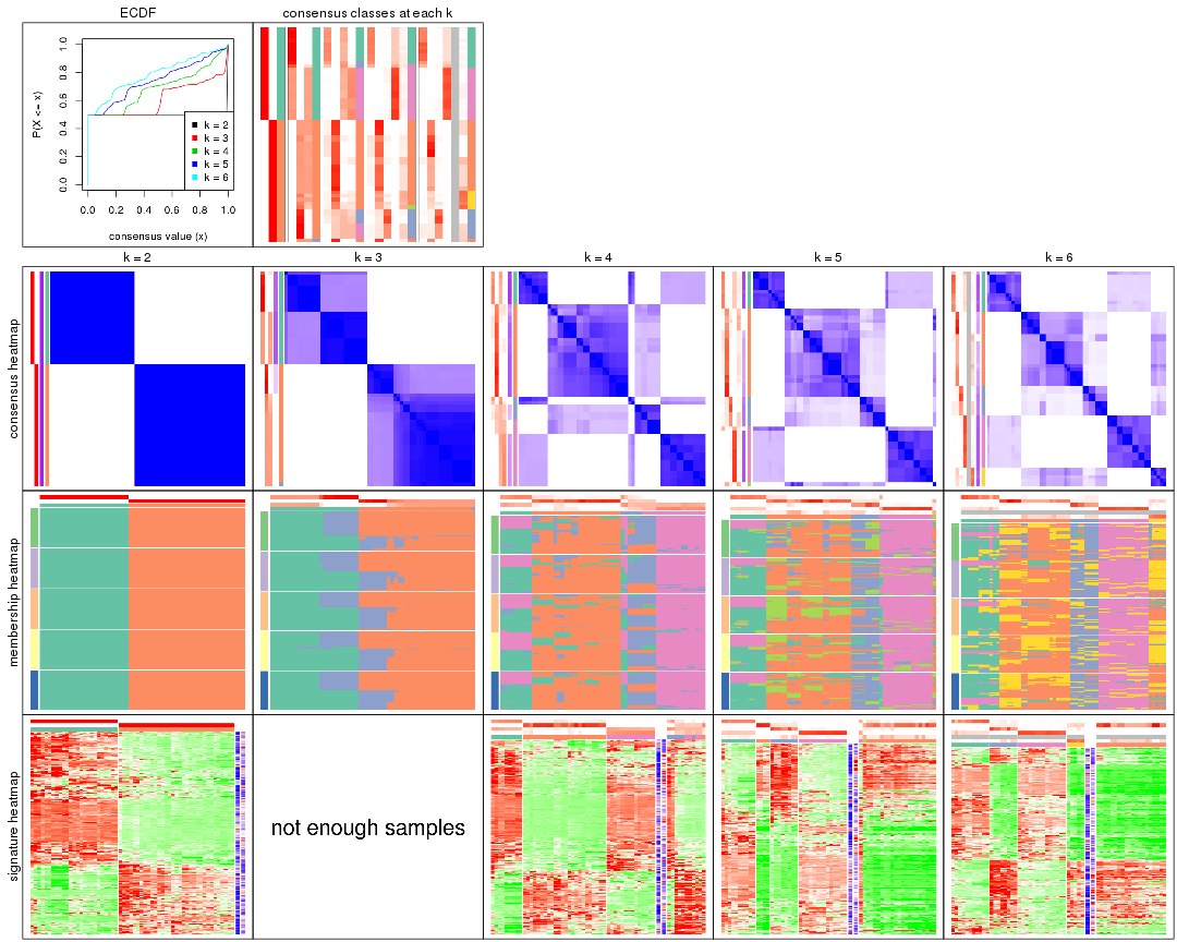
The plots are:
k and the heatmap of
predicted classes for each k.k.k.k.All the plots in panels can be made by individual functions and they are plotted later in this section.
select_partition_number() produces several plots showing different
statistics for choosing “optimized” k. There are following statistics:
k;k, the area increased is defined as \(A_k - A_{k-1}\).The detailed explanations of these statistics can be found in the cola vignette.
Generally speaking, lower PAC score, higher mean silhouette score or higher
concordance corresponds to better partition. Rand index and Jaccard index
measure how similar the current partition is compared to partition with k-1.
If they are too similar, we won't accept k is better than k-1.
select_partition_number(res)
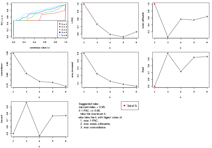
The numeric values for all these statistics can be obtained by get_stats().
get_stats(res)
#>   k 1-PAC mean_silhouette concordance area_increased  Rand Jaccard
#> 2 2 1.000          1.0000       1.000         0.4996 0.501   0.501
#> 3 3 0.732          0.0547       0.811         0.2243 0.981   0.961
#> 4 4 0.595          0.5655       0.737         0.1243 0.717   0.471
#> 5 5 0.563          0.5422       0.727         0.0827 0.923   0.764
#> 6 6 0.630          0.6403       0.692         0.0575 0.935   0.769
suggest_best_k() suggests the best \(k\) based on these statistics. The rules are as follows:
suggest_best_k(res)
#> [1] 2
Following shows the table of the partitions (You need to click the show/hide
code output link to see it). The membership matrix (columns with name p*)
is inferred by
clue::cl_consensus()
function with the SE method. Basically the value in the membership matrix
represents the probability to belong to a certain group. The finall class
label for an item is determined with the group with highest probability it
belongs to.
In get_classes() function, the entropy is calculated from the membership
matrix and the silhouette score is calculated from the consensus matrix.
cbind(get_classes(res, k = 2), get_membership(res, k = 2))
#>           class entropy silhouette p1 p2
#> ERR789082     2       0          1  0  1
#> ERR789083     2       0          1  0  1
#> ERR789191     2       0          1  0  1
#> ERR789192     2       0          1  0  1
#> ERR789213     1       0          1  1  0
#> ERR789385     1       0          1  1  0
#> ERR789393     1       0          1  1  0
#> ERR789394     1       0          1  1  0
#> ERR789193     2       0          1  0  1
#> ERR789194     2       0          1  0  1
#> ERR789195     2       0          1  0  1
#> ERR789196     2       0          1  0  1
#> ERR789388     1       0          1  1  0
#> ERR789197     2       0          1  0  1
#> ERR789198     2       0          1  0  1
#> ERR789214     1       0          1  1  0
#> ERR789397     1       0          1  1  0
#> ERR789398     1       0          1  1  0
#> ERR789199     2       0          1  0  1
#> ERR789200     2       0          1  0  1
#> ERR789201     2       0          1  0  1
#> ERR789202     2       0          1  0  1
#> ERR789215     1       0          1  1  0
#> ERR789203     2       0          1  0  1
#> ERR789204     2       0          1  0  1
#> ERR789383     1       0          1  1  0
#> ERR789205     2       0          1  0  1
#> ERR789206     2       0          1  0  1
#> ERR789399     1       0          1  1  0
#> ERR789400     1       0          1  1  0
#> ERR789207     2       0          1  0  1
#> ERR789208     2       0          1  0  1
#> ERR789209     2       0          1  0  1
#> ERR789210     2       0          1  0  1
#> ERR789211     2       0          1  0  1
#> ERR789212     2       0          1  0  1
#> ERR789386     1       0          1  1  0
#> ERR789076     2       0          1  0  1
#> ERR789077     2       0          1  0  1
#> ERR789384     1       0          1  1  0
#> ERR789078     2       0          1  0  1
#> ERR789079     2       0          1  0  1
#> ERR789216     1       0          1  1  0
#> ERR789080     2       0          1  0  1
#> ERR789387     1       0          1  1  0
#> ERR789081     2       0          1  0  1
#> ERR789064     2       0          1  0  1
#> ERR779485     2       0          1  0  1
#> ERR789065     2       0          1  0  1
#> ERR789401     1       0          1  1  0
#> ERR789402     1       0          1  1  0
#> ERR789403     1       0          1  1  0
#> ERR789389     1       0          1  1  0
#> ERR789395     1       0          1  1  0
#> ERR789396     1       0          1  1  0
#> ERR789390     1       0          1  1  0
#> ERR789391     1       0          1  1  0
#> ERR789392     1       0          1  1  0
cbind(get_classes(res, k = 3), get_membership(res, k = 3))
#>           class entropy silhouette    p1    p2    p3
#> ERR789082     2  0.6309    -0.9443 0.000 0.504 0.496
#> ERR789083     2  0.6309    -0.9443 0.000 0.504 0.496
#> ERR789191     2  0.6309    -0.9443 0.000 0.504 0.496
#> ERR789192     2  0.6309    -0.9443 0.000 0.504 0.496
#> ERR789213     1  0.6305     0.8316 0.516 0.000 0.484
#> ERR789385     1  0.6305     0.8316 0.516 0.000 0.484
#> ERR789393     1  0.6295     0.8327 0.528 0.000 0.472
#> ERR789394     1  0.6295     0.8327 0.528 0.000 0.472
#> ERR789193     2  0.1529     0.2577 0.000 0.960 0.040
#> ERR789194     2  0.1529     0.2577 0.000 0.960 0.040
#> ERR789195     2  0.6126    -0.4655 0.000 0.600 0.400
#> ERR789196     2  0.6126    -0.4655 0.000 0.600 0.400
#> ERR789388     1  0.6302     0.8321 0.520 0.000 0.480
#> ERR789197     2  0.6305    -0.9180 0.000 0.516 0.484
#> ERR789198     2  0.6305    -0.9180 0.000 0.516 0.484
#> ERR789214     1  0.6302     0.8321 0.520 0.000 0.480
#> ERR789397     1  0.6295     0.8327 0.528 0.000 0.472
#> ERR789398     1  0.6295     0.8327 0.528 0.000 0.472
#> ERR789199     2  0.6305    -0.9180 0.000 0.516 0.484
#> ERR789200     2  0.6305    -0.9180 0.000 0.516 0.484
#> ERR789201     2  0.6291    -0.8600 0.000 0.532 0.468
#> ERR789202     2  0.6291    -0.8600 0.000 0.532 0.468
#> ERR789215     1  0.0592     0.7679 0.988 0.000 0.012
#> ERR789203     2  0.0000     0.2631 0.000 1.000 0.000
#> ERR789204     2  0.0000     0.2631 0.000 1.000 0.000
#> ERR789383     1  0.0592     0.7679 0.988 0.000 0.012
#> ERR789205     2  0.0000     0.2631 0.000 1.000 0.000
#> ERR789206     2  0.0000     0.2631 0.000 1.000 0.000
#> ERR789399     1  0.0000     0.7692 1.000 0.000 0.000
#> ERR789400     1  0.0000     0.7692 1.000 0.000 0.000
#> ERR789207     2  0.6307    -0.9358 0.000 0.512 0.488
#> ERR789208     2  0.6307    -0.9358 0.000 0.512 0.488
#> ERR789209     2  0.6307    -0.9358 0.000 0.512 0.488
#> ERR789210     2  0.6307    -0.9358 0.000 0.512 0.488
#> ERR789211     2  0.6307    -0.9358 0.000 0.512 0.488
#> ERR789212     2  0.6307    -0.9358 0.000 0.512 0.488
#> ERR789386     1  0.6305     0.8316 0.516 0.000 0.484
#> ERR789076     2  0.5497    -0.0444 0.000 0.708 0.292
#> ERR789077     3  0.6309     0.0000 0.000 0.500 0.500
#> ERR789384     1  0.6305     0.8316 0.516 0.000 0.484
#> ERR789078     2  0.6302    -0.8909 0.000 0.520 0.480
#> ERR789079     2  0.6309    -0.9719 0.000 0.504 0.496
#> ERR789216     1  0.6305     0.8316 0.516 0.000 0.484
#> ERR789080     2  0.5810    -0.1723 0.000 0.664 0.336
#> ERR789387     1  0.0592     0.7679 0.988 0.000 0.012
#> ERR789081     2  0.6307    -0.9321 0.000 0.512 0.488
#> ERR789064     2  0.5948    -0.3239 0.000 0.640 0.360
#> ERR779485     2  0.0592     0.2610 0.000 0.988 0.012
#> ERR789065     2  0.0592     0.2610 0.000 0.988 0.012
#> ERR789401     1  0.0000     0.7692 1.000 0.000 0.000
#> ERR789402     1  0.0000     0.7692 1.000 0.000 0.000
#> ERR789403     1  0.0000     0.7692 1.000 0.000 0.000
#> ERR789389     1  0.4121     0.7931 0.832 0.000 0.168
#> ERR789395     1  0.0000     0.7692 1.000 0.000 0.000
#> ERR789396     1  0.0000     0.7692 1.000 0.000 0.000
#> ERR789390     1  0.6295     0.8327 0.528 0.000 0.472
#> ERR789391     1  0.6295     0.8327 0.528 0.000 0.472
#> ERR789392     1  0.6295     0.8327 0.528 0.000 0.472
cbind(get_classes(res, k = 4), get_membership(res, k = 4))
#>           class entropy silhouette    p1    p2    p3    p4
#> ERR789082     2  0.1792      0.835 0.068 0.932 0.000 0.000
#> ERR789083     2  0.1792      0.835 0.068 0.932 0.000 0.000
#> ERR789191     2  0.1940      0.834 0.076 0.924 0.000 0.000
#> ERR789192     2  0.1940      0.834 0.076 0.924 0.000 0.000
#> ERR789213     4  0.4933      0.539 0.000 0.000 0.432 0.568
#> ERR789385     4  0.4933      0.539 0.000 0.000 0.432 0.568
#> ERR789393     4  0.5376      0.536 0.016 0.000 0.396 0.588
#> ERR789394     4  0.5376      0.536 0.016 0.000 0.396 0.588
#> ERR789193     3  0.9603      0.349 0.132 0.304 0.340 0.224
#> ERR789194     3  0.9603      0.349 0.132 0.304 0.340 0.224
#> ERR789195     2  0.6212      0.704 0.168 0.712 0.092 0.028
#> ERR789196     2  0.6212      0.704 0.168 0.712 0.092 0.028
#> ERR789388     4  0.4888      0.540 0.000 0.000 0.412 0.588
#> ERR789197     2  0.3727      0.797 0.152 0.832 0.008 0.008
#> ERR789198     2  0.3727      0.797 0.152 0.832 0.008 0.008
#> ERR789214     4  0.4888      0.540 0.000 0.000 0.412 0.588
#> ERR789397     4  0.5284      0.540 0.016 0.000 0.368 0.616
#> ERR789398     4  0.5284      0.540 0.016 0.000 0.368 0.616
#> ERR789199     2  0.3534      0.800 0.148 0.840 0.008 0.004
#> ERR789200     2  0.3534      0.800 0.148 0.840 0.008 0.004
#> ERR789201     2  0.4300      0.787 0.020 0.832 0.036 0.112
#> ERR789202     2  0.4300      0.787 0.020 0.832 0.036 0.112
#> ERR789215     3  0.5000     -0.909 0.496 0.000 0.504 0.000
#> ERR789203     4  0.7853     -0.545 0.000 0.268 0.364 0.368
#> ERR789204     4  0.7853     -0.545 0.000 0.268 0.364 0.368
#> ERR789383     1  0.4999      0.901 0.508 0.000 0.492 0.000
#> ERR789205     4  0.7853     -0.545 0.000 0.268 0.364 0.368
#> ERR789206     4  0.7853     -0.545 0.000 0.268 0.364 0.368
#> ERR789399     1  0.4925      0.935 0.572 0.000 0.428 0.000
#> ERR789400     1  0.4925      0.935 0.572 0.000 0.428 0.000
#> ERR789207     2  0.1489      0.835 0.044 0.952 0.004 0.000
#> ERR789208     2  0.1398      0.836 0.040 0.956 0.004 0.000
#> ERR789209     2  0.1909      0.834 0.048 0.940 0.004 0.008
#> ERR789210     2  0.1909      0.834 0.048 0.940 0.004 0.008
#> ERR789211     2  0.1909      0.834 0.048 0.940 0.004 0.008
#> ERR789212     2  0.1909      0.834 0.048 0.940 0.004 0.008
#> ERR789386     4  0.4992      0.506 0.000 0.000 0.476 0.524
#> ERR789076     2  0.7555      0.483 0.064 0.624 0.176 0.136
#> ERR789077     2  0.1004      0.839 0.024 0.972 0.004 0.000
#> ERR789384     4  0.4977      0.522 0.000 0.000 0.460 0.540
#> ERR789078     2  0.4954      0.743 0.064 0.804 0.028 0.104
#> ERR789079     2  0.0657      0.838 0.012 0.984 0.004 0.000
#> ERR789216     4  0.4992      0.506 0.000 0.000 0.476 0.524
#> ERR789080     2  0.7097      0.563 0.064 0.668 0.140 0.128
#> ERR789387     1  0.4967      0.918 0.548 0.000 0.452 0.000
#> ERR789081     2  0.4457      0.763 0.064 0.828 0.016 0.092
#> ERR789064     2  0.7257      0.569 0.052 0.644 0.128 0.176
#> ERR779485     3  0.9332      0.384 0.092 0.256 0.368 0.284
#> ERR789065     3  0.9332      0.384 0.092 0.256 0.368 0.284
#> ERR789401     1  0.4776      0.945 0.624 0.000 0.376 0.000
#> ERR789402     1  0.4830      0.938 0.608 0.000 0.392 0.000
#> ERR789403     1  0.4776      0.945 0.624 0.000 0.376 0.000
#> ERR789389     3  0.6779     -0.744 0.324 0.000 0.560 0.116
#> ERR789395     1  0.4830      0.938 0.608 0.000 0.392 0.000
#> ERR789396     1  0.4830      0.938 0.608 0.000 0.392 0.000
#> ERR789390     4  0.5326      0.537 0.016 0.000 0.380 0.604
#> ERR789391     4  0.5326      0.537 0.016 0.000 0.380 0.604
#> ERR789392     4  0.5376      0.536 0.016 0.000 0.396 0.588
cbind(get_classes(res, k = 5), get_membership(res, k = 5))
#>           class entropy silhouette    p1    p2    p3    p4    p5
#> ERR789082     2  0.0771     0.5207 0.004 0.976 0.000 0.000 0.020
#> ERR789083     2  0.0771     0.5207 0.004 0.976 0.000 0.000 0.020
#> ERR789191     2  0.1106     0.5210 0.012 0.964 0.000 0.000 0.024
#> ERR789192     2  0.1106     0.5210 0.012 0.964 0.000 0.000 0.024
#> ERR789213     4  0.2729     0.8456 0.000 0.000 0.060 0.884 0.056
#> ERR789385     4  0.2729     0.8456 0.000 0.000 0.060 0.884 0.056
#> ERR789393     4  0.2196     0.8472 0.004 0.000 0.056 0.916 0.024
#> ERR789394     4  0.2196     0.8472 0.004 0.000 0.056 0.916 0.024
#> ERR789193     3  0.4812     0.6726 0.044 0.148 0.760 0.000 0.048
#> ERR789194     3  0.4812     0.6726 0.044 0.148 0.760 0.000 0.048
#> ERR789195     2  0.6526     0.3694 0.164 0.632 0.088 0.000 0.116
#> ERR789196     2  0.6526     0.3694 0.164 0.632 0.088 0.000 0.116
#> ERR789388     4  0.2172     0.8536 0.000 0.000 0.016 0.908 0.076
#> ERR789197     2  0.4735     0.4679 0.132 0.756 0.012 0.000 0.100
#> ERR789198     2  0.4735     0.4679 0.132 0.756 0.012 0.000 0.100
#> ERR789214     4  0.2172     0.8536 0.000 0.000 0.016 0.908 0.076
#> ERR789397     4  0.1808     0.8520 0.004 0.000 0.020 0.936 0.040
#> ERR789398     4  0.1808     0.8520 0.004 0.000 0.020 0.936 0.040
#> ERR789199     2  0.4435     0.4796 0.124 0.780 0.012 0.000 0.084
#> ERR789200     2  0.4435     0.4796 0.124 0.780 0.012 0.000 0.084
#> ERR789201     2  0.6199    -0.0252 0.048 0.584 0.064 0.000 0.304
#> ERR789202     2  0.6199    -0.0252 0.048 0.584 0.064 0.000 0.304
#> ERR789215     1  0.6177     0.8289 0.576 0.000 0.024 0.304 0.096
#> ERR789203     3  0.6733     0.6978 0.052 0.136 0.576 0.000 0.236
#> ERR789204     3  0.6733     0.6978 0.052 0.136 0.576 0.000 0.236
#> ERR789383     1  0.5213     0.8866 0.652 0.000 0.004 0.276 0.068
#> ERR789205     3  0.6797     0.6872 0.052 0.136 0.564 0.000 0.248
#> ERR789206     3  0.6797     0.6872 0.052 0.136 0.564 0.000 0.248
#> ERR789399     1  0.5294     0.8886 0.652 0.000 0.020 0.284 0.044
#> ERR789400     1  0.5294     0.8886 0.652 0.000 0.020 0.284 0.044
#> ERR789207     2  0.4177     0.4737 0.064 0.772 0.000 0.000 0.164
#> ERR789208     2  0.4177     0.4737 0.064 0.772 0.000 0.000 0.164
#> ERR789209     2  0.4385     0.4596 0.068 0.752 0.000 0.000 0.180
#> ERR789210     2  0.4385     0.4596 0.068 0.752 0.000 0.000 0.180
#> ERR789211     2  0.4385     0.4596 0.068 0.752 0.000 0.000 0.180
#> ERR789212     2  0.4385     0.4596 0.068 0.752 0.000 0.000 0.180
#> ERR789386     4  0.2720     0.8304 0.004 0.000 0.020 0.880 0.096
#> ERR789076     5  0.6304     0.0000 0.004 0.432 0.132 0.000 0.432
#> ERR789077     2  0.1908     0.4832 0.000 0.908 0.000 0.000 0.092
#> ERR789384     4  0.2505     0.8354 0.000 0.000 0.020 0.888 0.092
#> ERR789078     2  0.4696    -0.5669 0.000 0.556 0.016 0.000 0.428
#> ERR789079     2  0.2763     0.4326 0.004 0.848 0.000 0.000 0.148
#> ERR789216     4  0.2720     0.8304 0.004 0.000 0.020 0.880 0.096
#> ERR789080     2  0.6036    -0.9151 0.000 0.452 0.116 0.000 0.432
#> ERR789387     1  0.4758     0.8989 0.676 0.000 0.000 0.276 0.048
#> ERR789081     2  0.4730    -0.5259 0.004 0.568 0.012 0.000 0.416
#> ERR789064     2  0.6561    -0.7045 0.000 0.424 0.204 0.000 0.372
#> ERR779485     3  0.2280     0.7277 0.000 0.120 0.880 0.000 0.000
#> ERR789065     3  0.2280     0.7277 0.000 0.120 0.880 0.000 0.000
#> ERR789401     1  0.5076     0.9073 0.664 0.000 0.004 0.272 0.060
#> ERR789402     1  0.5597     0.8979 0.624 0.000 0.004 0.272 0.100
#> ERR789403     1  0.5076     0.9073 0.664 0.000 0.004 0.272 0.060
#> ERR789389     4  0.6616    -0.5212 0.412 0.000 0.016 0.436 0.136
#> ERR789395     1  0.5597     0.8979 0.624 0.000 0.004 0.272 0.100
#> ERR789396     1  0.5597     0.8979 0.624 0.000 0.004 0.272 0.100
#> ERR789390     4  0.2053     0.8500 0.004 0.000 0.024 0.924 0.048
#> ERR789391     4  0.2053     0.8500 0.004 0.000 0.024 0.924 0.048
#> ERR789392     4  0.2196     0.8472 0.004 0.000 0.056 0.916 0.024
cbind(get_classes(res, k = 6), get_membership(res, k = 6))
#>           class entropy silhouette    p1    p2    p3    p4 p5    p6
#> ERR789082     2  0.5531      0.494 0.016 0.636 0.008 0.000 NA 0.196
#> ERR789083     2  0.5531      0.494 0.016 0.636 0.008 0.000 NA 0.196
#> ERR789191     2  0.5478      0.497 0.016 0.644 0.008 0.000 NA 0.188
#> ERR789192     2  0.5478      0.497 0.016 0.644 0.008 0.000 NA 0.188
#> ERR789213     4  0.2500      0.832 0.000 0.000 0.012 0.868 NA 0.004
#> ERR789385     4  0.2500      0.832 0.000 0.000 0.012 0.868 NA 0.004
#> ERR789393     4  0.3354      0.833 0.012 0.000 0.012 0.820 NA 0.012
#> ERR789394     4  0.3354      0.833 0.012 0.000 0.012 0.820 NA 0.012
#> ERR789193     3  0.4964      0.601 0.040 0.072 0.740 0.000 NA 0.024
#> ERR789194     3  0.4964      0.601 0.040 0.072 0.740 0.000 NA 0.024
#> ERR789195     2  0.2980      0.408 0.020 0.872 0.040 0.000 NA 0.008
#> ERR789196     2  0.2980      0.408 0.020 0.872 0.040 0.000 NA 0.008
#> ERR789388     4  0.2705      0.829 0.000 0.000 0.004 0.872 NA 0.072
#> ERR789197     2  0.1065      0.464 0.008 0.964 0.008 0.000 NA 0.000
#> ERR789198     2  0.1065      0.464 0.008 0.964 0.008 0.000 NA 0.000
#> ERR789214     4  0.2705      0.829 0.000 0.000 0.004 0.872 NA 0.072
#> ERR789397     4  0.3460      0.831 0.012 0.000 0.004 0.832 NA 0.076
#> ERR789398     4  0.3460      0.831 0.012 0.000 0.004 0.832 NA 0.076
#> ERR789199     2  0.0146      0.471 0.000 0.996 0.000 0.000 NA 0.000
#> ERR789200     2  0.0146      0.471 0.000 0.996 0.000 0.000 NA 0.000
#> ERR789201     2  0.7418     -0.214 0.080 0.416 0.040 0.000 NA 0.332
#> ERR789202     2  0.7418     -0.214 0.080 0.416 0.040 0.000 NA 0.332
#> ERR789215     1  0.6269      0.757 0.528 0.000 0.012 0.240 NA 0.016
#> ERR789203     3  0.7397      0.669 0.100 0.096 0.516 0.000 NA 0.208
#> ERR789204     3  0.7397      0.669 0.100 0.096 0.516 0.000 NA 0.208
#> ERR789383     1  0.6143      0.816 0.600 0.000 0.008 0.180 NA 0.052
#> ERR789205     3  0.7454      0.657 0.096 0.096 0.500 0.000 NA 0.228
#> ERR789206     3  0.7454      0.657 0.096 0.096 0.500 0.000 NA 0.228
#> ERR789399     1  0.5146      0.824 0.640 0.000 0.004 0.184 NA 0.000
#> ERR789400     1  0.5146      0.824 0.640 0.000 0.004 0.184 NA 0.000
#> ERR789207     2  0.6042      0.436 0.000 0.436 0.008 0.000 NA 0.188
#> ERR789208     2  0.6042      0.436 0.000 0.436 0.008 0.000 NA 0.188
#> ERR789209     2  0.6099      0.420 0.000 0.420 0.008 0.000 NA 0.200
#> ERR789210     2  0.6099      0.420 0.000 0.420 0.008 0.000 NA 0.200
#> ERR789211     2  0.6099      0.420 0.000 0.420 0.008 0.000 NA 0.200
#> ERR789212     2  0.6099      0.420 0.000 0.420 0.008 0.000 NA 0.200
#> ERR789386     4  0.2846      0.799 0.000 0.000 0.024 0.868 NA 0.024
#> ERR789076     6  0.3915      0.857 0.004 0.188 0.052 0.000 NA 0.756
#> ERR789077     2  0.5488      0.440 0.008 0.604 0.008 0.000 NA 0.264
#> ERR789384     4  0.2684      0.808 0.000 0.000 0.024 0.880 NA 0.024
#> ERR789078     6  0.3445      0.827 0.000 0.244 0.012 0.000 NA 0.744
#> ERR789079     2  0.5423      0.318 0.004 0.516 0.000 0.000 NA 0.372
#> ERR789216     4  0.2846      0.799 0.000 0.000 0.024 0.868 NA 0.024
#> ERR789080     6  0.4344      0.853 0.012 0.184 0.060 0.000 NA 0.740
#> ERR789387     1  0.5919      0.829 0.644 0.000 0.016 0.180 NA 0.068
#> ERR789081     6  0.4052      0.771 0.012 0.260 0.000 0.000 NA 0.708
#> ERR789064     6  0.5047      0.751 0.000 0.208 0.156 0.000 NA 0.636
#> ERR779485     3  0.2344      0.685 0.004 0.076 0.892 0.000 NA 0.028
#> ERR789065     3  0.2277      0.684 0.000 0.076 0.892 0.000 NA 0.032
#> ERR789401     1  0.2809      0.848 0.824 0.000 0.000 0.168 NA 0.004
#> ERR789402     1  0.4296      0.835 0.756 0.000 0.016 0.168 NA 0.052
#> ERR789403     1  0.2809      0.848 0.824 0.000 0.000 0.168 NA 0.004
#> ERR789389     1  0.7444      0.502 0.360 0.000 0.028 0.360 NA 0.072
#> ERR789395     1  0.4296      0.835 0.756 0.000 0.016 0.168 NA 0.052
#> ERR789396     1  0.4296      0.835 0.756 0.000 0.016 0.168 NA 0.052
#> ERR789390     4  0.4080      0.830 0.016 0.000 0.028 0.796 NA 0.040
#> ERR789391     4  0.4080      0.830 0.016 0.000 0.028 0.796 NA 0.040
#> ERR789392     4  0.3354      0.833 0.012 0.000 0.012 0.820 NA 0.012
Heatmaps for the consensus matrix. It visualizes the probability of two samples to be in a same group.
consensus_heatmap(res, k = 2)

consensus_heatmap(res, k = 3)
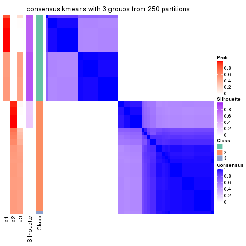
consensus_heatmap(res, k = 4)
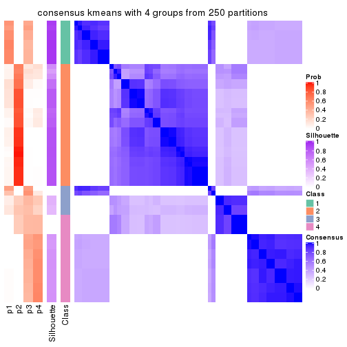
consensus_heatmap(res, k = 5)
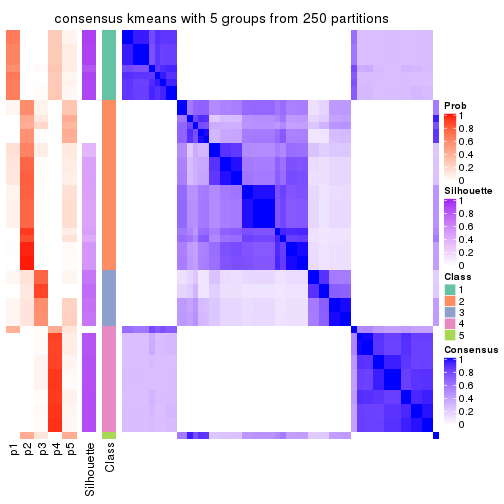
consensus_heatmap(res, k = 6)
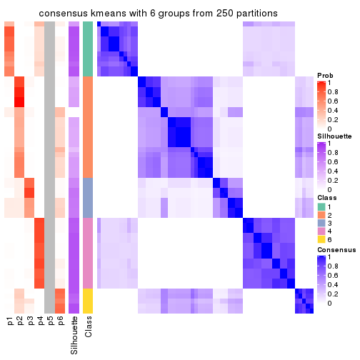
Heatmaps for the membership of samples in all partitions to see how consistent they are:
membership_heatmap(res, k = 2)

membership_heatmap(res, k = 3)
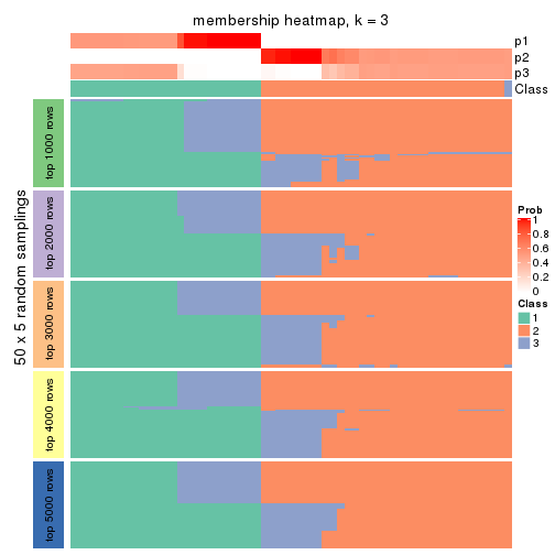
membership_heatmap(res, k = 4)
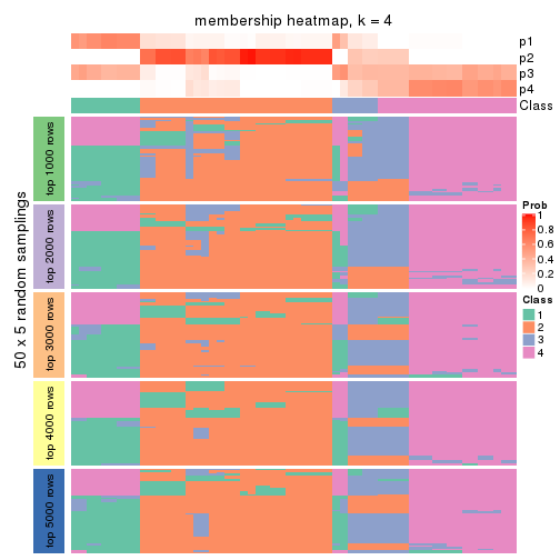
membership_heatmap(res, k = 5)
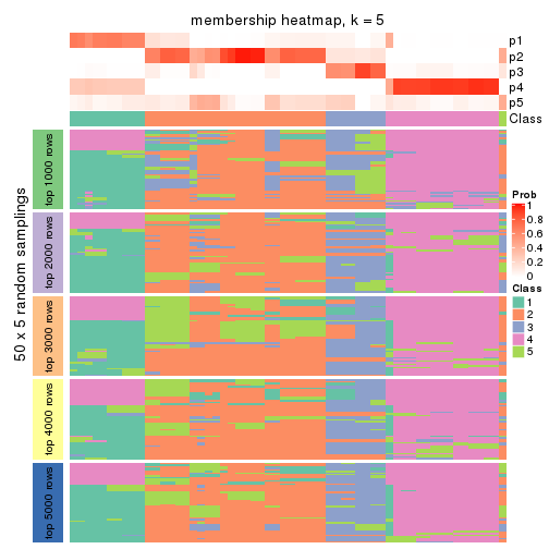
membership_heatmap(res, k = 6)
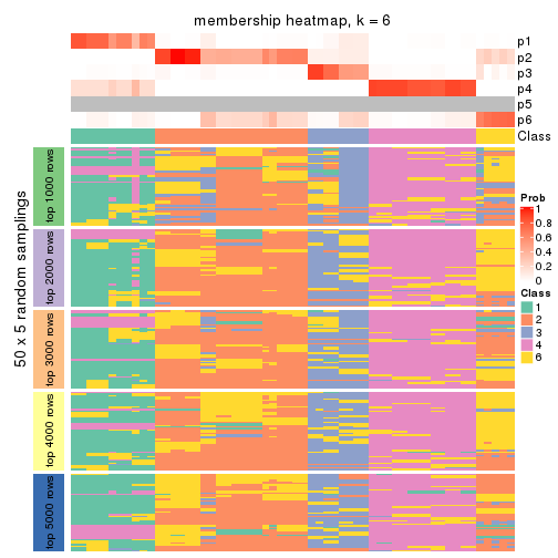
As soon as we have had the classes for columns, we can look for signatures which are significantly different between classes which can be candidate marks for certain classes. Following are the heatmaps for signatures.
Signature heatmaps where rows are scaled:
get_signatures(res, k = 2)

get_signatures(res, k = 3)

get_signatures(res, k = 4)
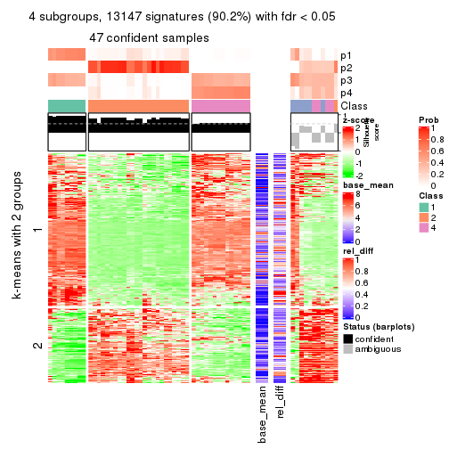
get_signatures(res, k = 5)
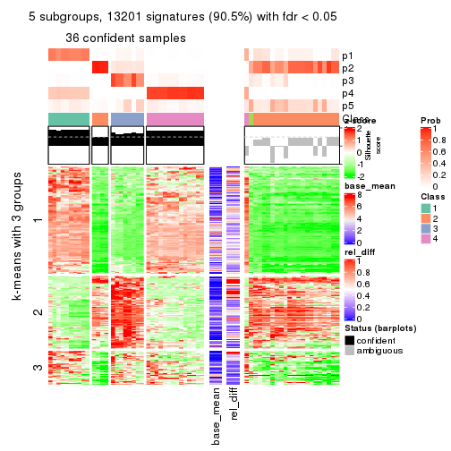
get_signatures(res, k = 6)
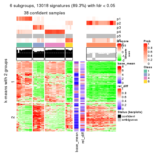
Signature heatmaps where rows are not scaled:
get_signatures(res, k = 2, scale_rows = FALSE)

get_signatures(res, k = 3, scale_rows = FALSE)

get_signatures(res, k = 4, scale_rows = FALSE)
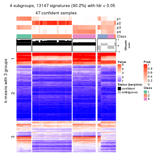
get_signatures(res, k = 5, scale_rows = FALSE)
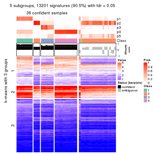
get_signatures(res, k = 6, scale_rows = FALSE)
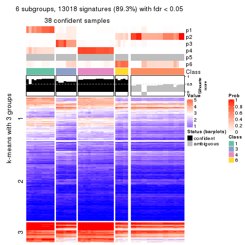
Compare the overlap of signatures from different k:
compare_signatures(res)
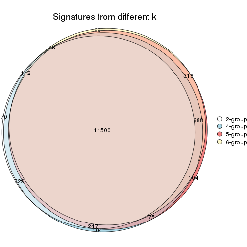
get_signature() returns a data frame invisibly. TO get the list of signatures, the function
call should be assigned to a variable explicitly. In following code, if plot argument is set
to FALSE, no heatmap is plotted while only the differential analysis is performed.
# code only for demonstration
tb = get_signature(res, k = ..., plot = FALSE)
An example of the output of tb is:
#>   which_row         fdr    mean_1    mean_2 scaled_mean_1 scaled_mean_2 km
#> 1        38 0.042760348  8.373488  9.131774    -0.5533452     0.5164555  1
#> 2        40 0.018707592  7.106213  8.469186    -0.6173731     0.5762149  1
#> 3        55 0.019134737 10.221463 11.207825    -0.6159697     0.5749050  1
#> 4        59 0.006059896  5.921854  7.869574    -0.6899429     0.6439467  1
#> 5        60 0.018055526  8.928898 10.211722    -0.6204761     0.5791110  1
#> 6        98 0.009384629 15.714769 14.887706     0.6635654    -0.6193277  2
...
The columns in tb are:
which_row: row indices corresponding to the input matrix.fdr: FDR for the differential test. mean_x: The mean value in group x.scaled_mean_x: The mean value in group x after rows are scaled.km: Row groups if k-means clustering is applied to rows.UMAP plot which shows how samples are separated.
dimension_reduction(res, k = 2, method = "UMAP")
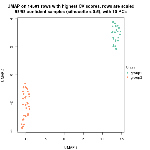
dimension_reduction(res, k = 3, method = "UMAP")
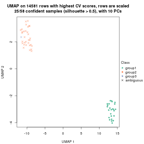
dimension_reduction(res, k = 4, method = "UMAP")
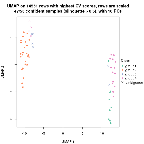
dimension_reduction(res, k = 5, method = "UMAP")
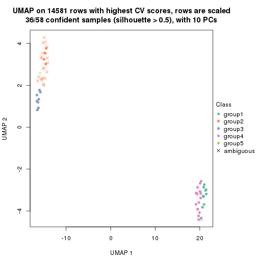
dimension_reduction(res, k = 6, method = "UMAP")
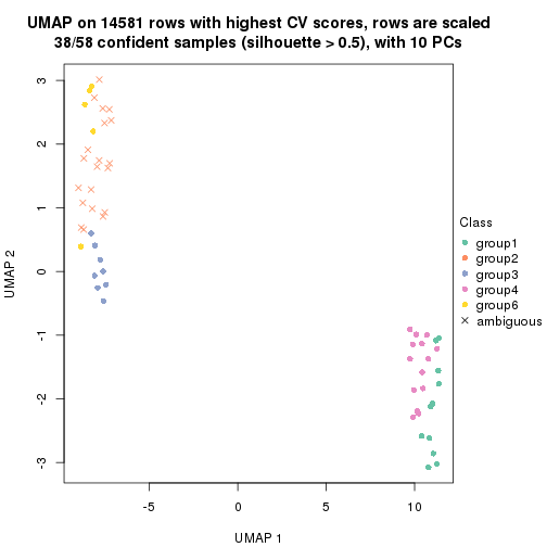
Following heatmap shows how subgroups are split when increasing k:
collect_classes(res)
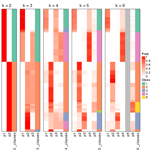
If matrix rows can be associated to genes, consider to use functional_enrichment(res,
...) to perform function enrichment for the signature genes. See this vignette for more detailed explanations.
The object with results only for a single top-value method and a single partition method can be extracted as:
res = res_list["CV", "skmeans"]
# you can also extract it by
# res = res_list["CV:skmeans"]
A summary of res and all the functions that can be applied to it:
res
#> A 'ConsensusPartition' object with k = 2, 3, 4, 5, 6.
#>   On a matrix with 14581 rows and 58 columns.
#>   Top rows (1000, 2000, 3000, 4000, 5000) are extracted by 'CV' method.
#>   Subgroups are detected by 'skmeans' method.
#>   Performed in total 1250 partitions by row resampling.
#>   Best k for subgroups seems to be 2.
#>
#> Following methods can be applied to this 'ConsensusPartition' object:
#>  [1] "cola_report"             "collect_classes"         "collect_plots"
#>  [4] "collect_stats"           "colnames"                "compare_signatures"
#>  [7] "consensus_heatmap"       "dimension_reduction"     "functional_enrichment"
#> [10] "get_anno_col"            "get_anno"                "get_classes"
#> [13] "get_consensus"           "get_matrix"              "get_membership"
#> [16] "get_param"               "get_signatures"          "get_stats"
#> [19] "is_best_k"               "is_stable_k"             "membership_heatmap"
#> [22] "ncol"                    "nrow"                    "plot_ecdf"
#> [25] "rownames"                "select_partition_number" "show"
#> [28] "suggest_best_k"          "test_to_known_factors"
collect_plots() function collects all the plots made from res for all k (number of partitions)
into one single page to provide an easy and fast comparison between different k.
collect_plots(res)
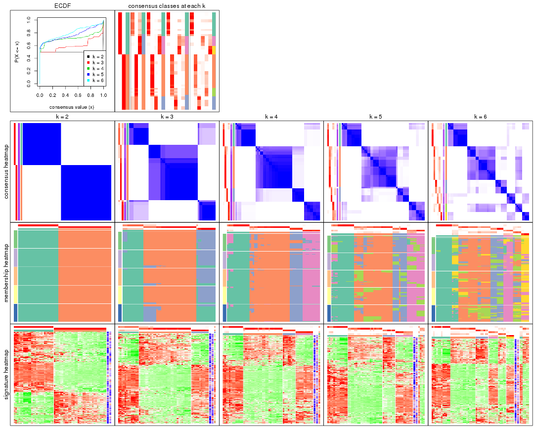
The plots are:
k and the heatmap of
predicted classes for each k.k.k.k.All the plots in panels can be made by individual functions and they are plotted later in this section.
select_partition_number() produces several plots showing different
statistics for choosing “optimized” k. There are following statistics:
k;k, the area increased is defined as \(A_k - A_{k-1}\).The detailed explanations of these statistics can be found in the cola vignette.
Generally speaking, lower PAC score, higher mean silhouette score or higher
concordance corresponds to better partition. Rand index and Jaccard index
measure how similar the current partition is compared to partition with k-1.
If they are too similar, we won't accept k is better than k-1.
select_partition_number(res)
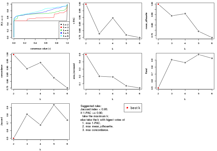
The numeric values for all these statistics can be obtained by get_stats().
get_stats(res)
#>   k 1-PAC mean_silhouette concordance area_increased  Rand Jaccard
#> 2 2 1.000           1.000       1.000         0.4996 0.501   0.501
#> 3 3 0.777           0.888       0.894         0.2027 0.906   0.812
#> 4 4 0.896           0.909       0.940         0.1933 0.864   0.673
#> 5 5 0.768           0.740       0.827         0.0726 0.981   0.934
#> 6 6 0.747           0.679       0.751         0.0434 0.926   0.736
suggest_best_k() suggests the best \(k\) based on these statistics. The rules are as follows:
suggest_best_k(res)
#> [1] 2
Following shows the table of the partitions (You need to click the show/hide
code output link to see it). The membership matrix (columns with name p*)
is inferred by
clue::cl_consensus()
function with the SE method. Basically the value in the membership matrix
represents the probability to belong to a certain group. The finall class
label for an item is determined with the group with highest probability it
belongs to.
In get_classes() function, the entropy is calculated from the membership
matrix and the silhouette score is calculated from the consensus matrix.
cbind(get_classes(res, k = 2), get_membership(res, k = 2))
#>           class entropy silhouette p1 p2
#> ERR789082     2       0          1  0  1
#> ERR789083     2       0          1  0  1
#> ERR789191     2       0          1  0  1
#> ERR789192     2       0          1  0  1
#> ERR789213     1       0          1  1  0
#> ERR789385     1       0          1  1  0
#> ERR789393     1       0          1  1  0
#> ERR789394     1       0          1  1  0
#> ERR789193     2       0          1  0  1
#> ERR789194     2       0          1  0  1
#> ERR789195     2       0          1  0  1
#> ERR789196     2       0          1  0  1
#> ERR789388     1       0          1  1  0
#> ERR789197     2       0          1  0  1
#> ERR789198     2       0          1  0  1
#> ERR789214     1       0          1  1  0
#> ERR789397     1       0          1  1  0
#> ERR789398     1       0          1  1  0
#> ERR789199     2       0          1  0  1
#> ERR789200     2       0          1  0  1
#> ERR789201     2       0          1  0  1
#> ERR789202     2       0          1  0  1
#> ERR789215     1       0          1  1  0
#> ERR789203     2       0          1  0  1
#> ERR789204     2       0          1  0  1
#> ERR789383     1       0          1  1  0
#> ERR789205     2       0          1  0  1
#> ERR789206     2       0          1  0  1
#> ERR789399     1       0          1  1  0
#> ERR789400     1       0          1  1  0
#> ERR789207     2       0          1  0  1
#> ERR789208     2       0          1  0  1
#> ERR789209     2       0          1  0  1
#> ERR789210     2       0          1  0  1
#> ERR789211     2       0          1  0  1
#> ERR789212     2       0          1  0  1
#> ERR789386     1       0          1  1  0
#> ERR789076     2       0          1  0  1
#> ERR789077     2       0          1  0  1
#> ERR789384     1       0          1  1  0
#> ERR789078     2       0          1  0  1
#> ERR789079     2       0          1  0  1
#> ERR789216     1       0          1  1  0
#> ERR789080     2       0          1  0  1
#> ERR789387     1       0          1  1  0
#> ERR789081     2       0          1  0  1
#> ERR789064     2       0          1  0  1
#> ERR779485     2       0          1  0  1
#> ERR789065     2       0          1  0  1
#> ERR789401     1       0          1  1  0
#> ERR789402     1       0          1  1  0
#> ERR789403     1       0          1  1  0
#> ERR789389     1       0          1  1  0
#> ERR789395     1       0          1  1  0
#> ERR789396     1       0          1  1  0
#> ERR789390     1       0          1  1  0
#> ERR789391     1       0          1  1  0
#> ERR789392     1       0          1  1  0
cbind(get_classes(res, k = 3), get_membership(res, k = 3))
#>           class entropy silhouette    p1    p2    p3
#> ERR789082     2  0.0000      0.941 0.000 1.000 0.000
#> ERR789083     2  0.0000      0.941 0.000 1.000 0.000
#> ERR789191     2  0.0000      0.941 0.000 1.000 0.000
#> ERR789192     2  0.0000      0.941 0.000 1.000 0.000
#> ERR789213     3  0.0000      0.931 0.000 0.000 1.000
#> ERR789385     3  0.0000      0.931 0.000 0.000 1.000
#> ERR789393     3  0.0000      0.931 0.000 0.000 1.000
#> ERR789394     3  0.0000      0.931 0.000 0.000 1.000
#> ERR789193     2  0.5098      0.822 0.248 0.752 0.000
#> ERR789194     2  0.5098      0.822 0.248 0.752 0.000
#> ERR789195     2  0.0237      0.941 0.004 0.996 0.000
#> ERR789196     2  0.0237      0.941 0.004 0.996 0.000
#> ERR789388     3  0.0000      0.931 0.000 0.000 1.000
#> ERR789197     2  0.0000      0.941 0.000 1.000 0.000
#> ERR789198     2  0.0000      0.941 0.000 1.000 0.000
#> ERR789214     3  0.0000      0.931 0.000 0.000 1.000
#> ERR789397     3  0.0000      0.931 0.000 0.000 1.000
#> ERR789398     3  0.0000      0.931 0.000 0.000 1.000
#> ERR789199     2  0.0000      0.941 0.000 1.000 0.000
#> ERR789200     2  0.0000      0.941 0.000 1.000 0.000
#> ERR789201     2  0.0000      0.941 0.000 1.000 0.000
#> ERR789202     2  0.0000      0.941 0.000 1.000 0.000
#> ERR789215     1  0.5098      0.942 0.752 0.000 0.248
#> ERR789203     2  0.5098      0.822 0.248 0.752 0.000
#> ERR789204     2  0.5098      0.822 0.248 0.752 0.000
#> ERR789383     1  0.5098      0.942 0.752 0.000 0.248
#> ERR789205     2  0.5098      0.822 0.248 0.752 0.000
#> ERR789206     2  0.5098      0.822 0.248 0.752 0.000
#> ERR789399     1  0.5098      0.942 0.752 0.000 0.248
#> ERR789400     1  0.5098      0.942 0.752 0.000 0.248
#> ERR789207     2  0.0000      0.941 0.000 1.000 0.000
#> ERR789208     2  0.0000      0.941 0.000 1.000 0.000
#> ERR789209     2  0.0000      0.941 0.000 1.000 0.000
#> ERR789210     2  0.0000      0.941 0.000 1.000 0.000
#> ERR789211     2  0.0000      0.941 0.000 1.000 0.000
#> ERR789212     2  0.0000      0.941 0.000 1.000 0.000
#> ERR789386     1  0.6154      0.759 0.592 0.000 0.408
#> ERR789076     2  0.2261      0.917 0.068 0.932 0.000
#> ERR789077     2  0.0000      0.941 0.000 1.000 0.000
#> ERR789384     3  0.6235     -0.397 0.436 0.000 0.564
#> ERR789078     2  0.0237      0.941 0.004 0.996 0.000
#> ERR789079     2  0.0000      0.941 0.000 1.000 0.000
#> ERR789216     1  0.6154      0.759 0.592 0.000 0.408
#> ERR789080     2  0.2066      0.920 0.060 0.940 0.000
#> ERR789387     1  0.5098      0.942 0.752 0.000 0.248
#> ERR789081     2  0.0000      0.941 0.000 1.000 0.000
#> ERR789064     2  0.1643      0.926 0.044 0.956 0.000
#> ERR779485     2  0.5098      0.822 0.248 0.752 0.000
#> ERR789065     2  0.5098      0.822 0.248 0.752 0.000
#> ERR789401     1  0.5098      0.942 0.752 0.000 0.248
#> ERR789402     1  0.5098      0.942 0.752 0.000 0.248
#> ERR789403     1  0.5098      0.942 0.752 0.000 0.248
#> ERR789389     1  0.6126      0.772 0.600 0.000 0.400
#> ERR789395     1  0.5098      0.942 0.752 0.000 0.248
#> ERR789396     1  0.5098      0.942 0.752 0.000 0.248
#> ERR789390     3  0.1529      0.894 0.040 0.000 0.960
#> ERR789391     3  0.1529      0.894 0.040 0.000 0.960
#> ERR789392     3  0.0000      0.931 0.000 0.000 1.000
cbind(get_classes(res, k = 4), get_membership(res, k = 4))
#>           class entropy silhouette    p1    p2    p3    p4
#> ERR789082     2  0.0000      0.941 0.000 1.000 0.000 0.000
#> ERR789083     2  0.0000      0.941 0.000 1.000 0.000 0.000
#> ERR789191     2  0.0188      0.941 0.000 0.996 0.000 0.004
#> ERR789192     2  0.0188      0.941 0.000 0.996 0.000 0.004
#> ERR789213     4  0.2089      0.964 0.020 0.000 0.048 0.932
#> ERR789385     4  0.2089      0.964 0.020 0.000 0.048 0.932
#> ERR789393     4  0.1724      0.968 0.020 0.000 0.032 0.948
#> ERR789394     4  0.1724      0.968 0.020 0.000 0.032 0.948
#> ERR789193     3  0.2125      0.986 0.000 0.076 0.920 0.004
#> ERR789194     3  0.2125      0.986 0.000 0.076 0.920 0.004
#> ERR789195     2  0.3300      0.820 0.000 0.848 0.144 0.008
#> ERR789196     2  0.3300      0.820 0.000 0.848 0.144 0.008
#> ERR789388     4  0.1610      0.967 0.016 0.000 0.032 0.952
#> ERR789197     2  0.0804      0.936 0.000 0.980 0.012 0.008
#> ERR789198     2  0.0804      0.936 0.000 0.980 0.012 0.008
#> ERR789214     4  0.1610      0.967 0.016 0.000 0.032 0.952
#> ERR789397     4  0.1182      0.966 0.016 0.000 0.016 0.968
#> ERR789398     4  0.1182      0.966 0.016 0.000 0.016 0.968
#> ERR789199     2  0.0336      0.939 0.000 0.992 0.000 0.008
#> ERR789200     2  0.0336      0.939 0.000 0.992 0.000 0.008
#> ERR789201     2  0.1022      0.930 0.000 0.968 0.032 0.000
#> ERR789202     2  0.1118      0.928 0.000 0.964 0.036 0.000
#> ERR789215     1  0.0000      0.921 1.000 0.000 0.000 0.000
#> ERR789203     3  0.1716      0.994 0.000 0.064 0.936 0.000
#> ERR789204     3  0.1716      0.994 0.000 0.064 0.936 0.000
#> ERR789383     1  0.0000      0.921 1.000 0.000 0.000 0.000
#> ERR789205     3  0.1716      0.994 0.000 0.064 0.936 0.000
#> ERR789206     3  0.1716      0.994 0.000 0.064 0.936 0.000
#> ERR789399     1  0.0000      0.921 1.000 0.000 0.000 0.000
#> ERR789400     1  0.0000      0.921 1.000 0.000 0.000 0.000
#> ERR789207     2  0.0000      0.941 0.000 1.000 0.000 0.000
#> ERR789208     2  0.0000      0.941 0.000 1.000 0.000 0.000
#> ERR789209     2  0.0000      0.941 0.000 1.000 0.000 0.000
#> ERR789210     2  0.0000      0.941 0.000 1.000 0.000 0.000
#> ERR789211     2  0.0000      0.941 0.000 1.000 0.000 0.000
#> ERR789212     2  0.0000      0.941 0.000 1.000 0.000 0.000
#> ERR789386     1  0.4508      0.765 0.780 0.000 0.036 0.184
#> ERR789076     2  0.4761      0.503 0.000 0.664 0.332 0.004
#> ERR789077     2  0.0000      0.941 0.000 1.000 0.000 0.000
#> ERR789384     1  0.5793      0.392 0.580 0.000 0.036 0.384
#> ERR789078     2  0.1109      0.927 0.000 0.968 0.028 0.004
#> ERR789079     2  0.0000      0.941 0.000 1.000 0.000 0.000
#> ERR789216     1  0.4466      0.769 0.784 0.000 0.036 0.180
#> ERR789080     2  0.3982      0.714 0.000 0.776 0.220 0.004
#> ERR789387     1  0.0000      0.921 1.000 0.000 0.000 0.000
#> ERR789081     2  0.0779      0.934 0.000 0.980 0.016 0.004
#> ERR789064     2  0.4483      0.635 0.000 0.712 0.284 0.004
#> ERR779485     3  0.1902      0.994 0.000 0.064 0.932 0.004
#> ERR789065     3  0.1902      0.994 0.000 0.064 0.932 0.004
#> ERR789401     1  0.0000      0.921 1.000 0.000 0.000 0.000
#> ERR789402     1  0.0000      0.921 1.000 0.000 0.000 0.000
#> ERR789403     1  0.0000      0.921 1.000 0.000 0.000 0.000
#> ERR789389     1  0.3787      0.822 0.840 0.000 0.036 0.124
#> ERR789395     1  0.0000      0.921 1.000 0.000 0.000 0.000
#> ERR789396     1  0.0000      0.921 1.000 0.000 0.000 0.000
#> ERR789390     4  0.1637      0.948 0.060 0.000 0.000 0.940
#> ERR789391     4  0.1637      0.948 0.060 0.000 0.000 0.940
#> ERR789392     4  0.1724      0.968 0.020 0.000 0.032 0.948
cbind(get_classes(res, k = 5), get_membership(res, k = 5))
#>           class entropy silhouette    p1    p2    p3    p4    p5
#> ERR789082     2  0.1965      0.800 0.000 0.904 0.000 0.000 0.096
#> ERR789083     2  0.1965      0.800 0.000 0.904 0.000 0.000 0.096
#> ERR789191     2  0.2020      0.799 0.000 0.900 0.000 0.000 0.100
#> ERR789192     2  0.2020      0.799 0.000 0.900 0.000 0.000 0.100
#> ERR789213     4  0.0404      0.768 0.000 0.000 0.000 0.988 0.012
#> ERR789385     4  0.0404      0.768 0.000 0.000 0.000 0.988 0.012
#> ERR789393     4  0.1544      0.789 0.000 0.000 0.000 0.932 0.068
#> ERR789394     4  0.1544      0.789 0.000 0.000 0.000 0.932 0.068
#> ERR789193     3  0.4550      0.750 0.000 0.036 0.688 0.000 0.276
#> ERR789194     3  0.4550      0.750 0.000 0.036 0.688 0.000 0.276
#> ERR789195     2  0.5673      0.607 0.000 0.632 0.184 0.000 0.184
#> ERR789196     2  0.5673      0.607 0.000 0.632 0.184 0.000 0.184
#> ERR789388     4  0.4238      0.799 0.004 0.000 0.000 0.628 0.368
#> ERR789197     2  0.3953      0.759 0.000 0.784 0.048 0.000 0.168
#> ERR789198     2  0.3953      0.759 0.000 0.784 0.048 0.000 0.168
#> ERR789214     4  0.4238      0.799 0.004 0.000 0.000 0.628 0.368
#> ERR789397     4  0.4397      0.802 0.004 0.000 0.000 0.564 0.432
#> ERR789398     4  0.4397      0.802 0.004 0.000 0.000 0.564 0.432
#> ERR789199     2  0.3810      0.763 0.000 0.792 0.040 0.000 0.168
#> ERR789200     2  0.3810      0.763 0.000 0.792 0.040 0.000 0.168
#> ERR789201     2  0.3910      0.641 0.000 0.720 0.272 0.000 0.008
#> ERR789202     2  0.3957      0.632 0.000 0.712 0.280 0.000 0.008
#> ERR789215     1  0.0404      0.890 0.988 0.000 0.000 0.000 0.012
#> ERR789203     3  0.0162      0.789 0.000 0.004 0.996 0.000 0.000
#> ERR789204     3  0.0162      0.789 0.000 0.004 0.996 0.000 0.000
#> ERR789383     1  0.0404      0.890 0.988 0.000 0.000 0.000 0.012
#> ERR789205     3  0.0290      0.788 0.000 0.008 0.992 0.000 0.000
#> ERR789206     3  0.0290      0.788 0.000 0.008 0.992 0.000 0.000
#> ERR789399     1  0.0000      0.892 1.000 0.000 0.000 0.000 0.000
#> ERR789400     1  0.0000      0.892 1.000 0.000 0.000 0.000 0.000
#> ERR789207     2  0.0579      0.803 0.000 0.984 0.008 0.000 0.008
#> ERR789208     2  0.0579      0.803 0.000 0.984 0.008 0.000 0.008
#> ERR789209     2  0.0798      0.802 0.000 0.976 0.016 0.000 0.008
#> ERR789210     2  0.0798      0.802 0.000 0.976 0.016 0.000 0.008
#> ERR789211     2  0.0798      0.802 0.000 0.976 0.016 0.000 0.008
#> ERR789212     2  0.0798      0.802 0.000 0.976 0.016 0.000 0.008
#> ERR789386     1  0.4974      0.647 0.660 0.000 0.004 0.288 0.048
#> ERR789076     2  0.5658      0.200 0.000 0.512 0.408 0.000 0.080
#> ERR789077     2  0.1608      0.804 0.000 0.928 0.000 0.000 0.072
#> ERR789384     1  0.5352      0.452 0.556 0.000 0.004 0.392 0.048
#> ERR789078     2  0.5039      0.547 0.000 0.676 0.244 0.000 0.080
#> ERR789079     2  0.0162      0.804 0.000 0.996 0.000 0.000 0.004
#> ERR789216     1  0.4932      0.658 0.668 0.000 0.004 0.280 0.048
#> ERR789080     2  0.5589      0.304 0.000 0.548 0.372 0.000 0.080
#> ERR789387     1  0.0510      0.890 0.984 0.000 0.000 0.000 0.016
#> ERR789081     2  0.4818      0.590 0.000 0.708 0.212 0.000 0.080
#> ERR789064     3  0.5725     -0.146 0.000 0.428 0.488 0.000 0.084
#> ERR779485     3  0.3766      0.759 0.000 0.004 0.728 0.000 0.268
#> ERR789065     3  0.3715      0.762 0.000 0.004 0.736 0.000 0.260
#> ERR789401     1  0.0162      0.892 0.996 0.000 0.000 0.000 0.004
#> ERR789402     1  0.0162      0.892 0.996 0.000 0.000 0.000 0.004
#> ERR789403     1  0.0162      0.892 0.996 0.000 0.000 0.000 0.004
#> ERR789389     1  0.4450      0.731 0.736 0.000 0.004 0.216 0.044
#> ERR789395     1  0.0162      0.892 0.996 0.000 0.000 0.000 0.004
#> ERR789396     1  0.0162      0.892 0.996 0.000 0.000 0.000 0.004
#> ERR789390     4  0.5598      0.792 0.080 0.000 0.000 0.544 0.376
#> ERR789391     4  0.5598      0.792 0.080 0.000 0.000 0.544 0.376
#> ERR789392     4  0.1544      0.789 0.000 0.000 0.000 0.932 0.068
cbind(get_classes(res, k = 6), get_membership(res, k = 6))
#>           class entropy silhouette    p1    p2    p3    p4    p5    p6
#> ERR789082     2  0.3103     0.6413 0.000 0.784 0.000 0.008 0.208 0.000
#> ERR789083     2  0.3133     0.6407 0.000 0.780 0.000 0.008 0.212 0.000
#> ERR789191     2  0.3043     0.6416 0.000 0.792 0.000 0.008 0.200 0.000
#> ERR789192     2  0.3043     0.6416 0.000 0.792 0.000 0.008 0.200 0.000
#> ERR789213     6  0.1643     0.8964 0.000 0.000 0.000 0.068 0.008 0.924
#> ERR789385     6  0.1643     0.8964 0.000 0.000 0.000 0.068 0.008 0.924
#> ERR789393     6  0.0146     0.9294 0.000 0.000 0.000 0.004 0.000 0.996
#> ERR789394     6  0.0146     0.9294 0.000 0.000 0.000 0.004 0.000 0.996
#> ERR789193     3  0.1053     0.7121 0.000 0.020 0.964 0.012 0.004 0.000
#> ERR789194     3  0.1053     0.7121 0.000 0.020 0.964 0.012 0.004 0.000
#> ERR789195     2  0.3635     0.4306 0.000 0.804 0.120 0.068 0.008 0.000
#> ERR789196     2  0.3718     0.4191 0.000 0.796 0.128 0.068 0.008 0.000
#> ERR789388     4  0.3101     0.8211 0.000 0.000 0.000 0.756 0.000 0.244
#> ERR789197     2  0.1686     0.5570 0.000 0.924 0.012 0.064 0.000 0.000
#> ERR789198     2  0.1686     0.5570 0.000 0.924 0.012 0.064 0.000 0.000
#> ERR789214     4  0.3101     0.8211 0.000 0.000 0.000 0.756 0.000 0.244
#> ERR789397     4  0.3482     0.8388 0.000 0.000 0.000 0.684 0.000 0.316
#> ERR789398     4  0.3482     0.8388 0.000 0.000 0.000 0.684 0.000 0.316
#> ERR789199     2  0.1686     0.5570 0.000 0.924 0.012 0.064 0.000 0.000
#> ERR789200     2  0.1686     0.5570 0.000 0.924 0.012 0.064 0.000 0.000
#> ERR789201     2  0.5700    -0.0756 0.000 0.464 0.036 0.068 0.432 0.000
#> ERR789202     2  0.5700    -0.0756 0.000 0.464 0.036 0.068 0.432 0.000
#> ERR789215     1  0.0547     0.8456 0.980 0.000 0.000 0.000 0.020 0.000
#> ERR789203     3  0.5293     0.6703 0.000 0.032 0.576 0.052 0.340 0.000
#> ERR789204     3  0.5293     0.6703 0.000 0.032 0.576 0.052 0.340 0.000
#> ERR789383     1  0.0547     0.8456 0.980 0.000 0.000 0.000 0.020 0.000
#> ERR789205     3  0.5327     0.6611 0.000 0.032 0.564 0.052 0.352 0.000
#> ERR789206     3  0.5316     0.6651 0.000 0.032 0.568 0.052 0.348 0.000
#> ERR789399     1  0.0000     0.8489 1.000 0.000 0.000 0.000 0.000 0.000
#> ERR789400     1  0.0000     0.8489 1.000 0.000 0.000 0.000 0.000 0.000
#> ERR789207     2  0.4669     0.5984 0.000 0.648 0.004 0.064 0.284 0.000
#> ERR789208     2  0.4669     0.5984 0.000 0.648 0.004 0.064 0.284 0.000
#> ERR789209     2  0.4723     0.5879 0.000 0.636 0.004 0.064 0.296 0.000
#> ERR789210     2  0.4723     0.5879 0.000 0.636 0.004 0.064 0.296 0.000
#> ERR789211     2  0.4723     0.5879 0.000 0.636 0.004 0.064 0.296 0.000
#> ERR789212     2  0.4723     0.5879 0.000 0.636 0.004 0.064 0.296 0.000
#> ERR789386     1  0.6748     0.5004 0.524 0.000 0.000 0.132 0.152 0.192
#> ERR789076     5  0.4131     0.8074 0.000 0.180 0.072 0.004 0.744 0.000
#> ERR789077     2  0.3323     0.6306 0.000 0.752 0.000 0.008 0.240 0.000
#> ERR789384     1  0.7058     0.3841 0.460 0.000 0.000 0.140 0.152 0.248
#> ERR789078     5  0.3354     0.7967 0.000 0.240 0.004 0.004 0.752 0.000
#> ERR789079     2  0.3729     0.5912 0.000 0.692 0.000 0.012 0.296 0.000
#> ERR789216     1  0.6801     0.4899 0.516 0.000 0.000 0.136 0.152 0.196
#> ERR789080     5  0.3593     0.8219 0.000 0.180 0.020 0.016 0.784 0.000
#> ERR789387     1  0.0603     0.8458 0.980 0.000 0.000 0.004 0.016 0.000
#> ERR789081     5  0.3855     0.7342 0.000 0.276 0.004 0.016 0.704 0.000
#> ERR789064     5  0.5001     0.6254 0.000 0.160 0.196 0.000 0.644 0.000
#> ERR779485     3  0.0260     0.7253 0.000 0.000 0.992 0.000 0.008 0.000
#> ERR789065     3  0.0458     0.7266 0.000 0.000 0.984 0.000 0.016 0.000
#> ERR789401     1  0.0000     0.8489 1.000 0.000 0.000 0.000 0.000 0.000
#> ERR789402     1  0.0000     0.8489 1.000 0.000 0.000 0.000 0.000 0.000
#> ERR789403     1  0.0000     0.8489 1.000 0.000 0.000 0.000 0.000 0.000
#> ERR789389     1  0.6453     0.5536 0.568 0.000 0.000 0.124 0.152 0.156
#> ERR789395     1  0.0000     0.8489 1.000 0.000 0.000 0.000 0.000 0.000
#> ERR789396     1  0.0000     0.8489 1.000 0.000 0.000 0.000 0.000 0.000
#> ERR789390     4  0.5808     0.7482 0.128 0.000 0.000 0.508 0.016 0.348
#> ERR789391     4  0.5808     0.7482 0.128 0.000 0.000 0.508 0.016 0.348
#> ERR789392     6  0.0146     0.9294 0.000 0.000 0.000 0.004 0.000 0.996
Heatmaps for the consensus matrix. It visualizes the probability of two samples to be in a same group.
consensus_heatmap(res, k = 2)

consensus_heatmap(res, k = 3)
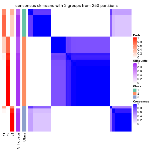
consensus_heatmap(res, k = 4)
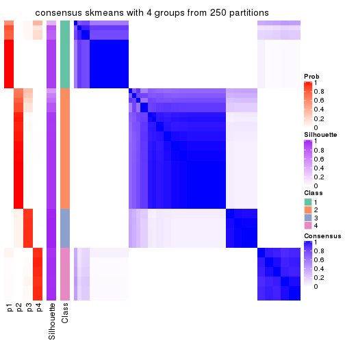
consensus_heatmap(res, k = 5)
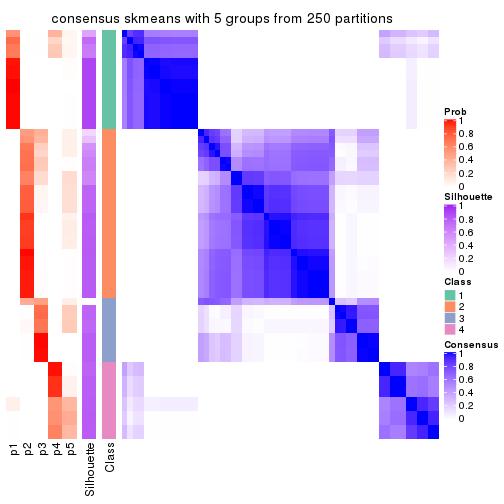
consensus_heatmap(res, k = 6)
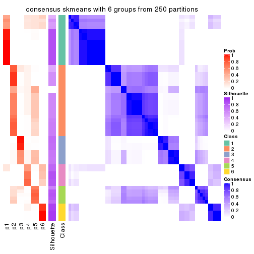
Heatmaps for the membership of samples in all partitions to see how consistent they are:
membership_heatmap(res, k = 2)

membership_heatmap(res, k = 3)
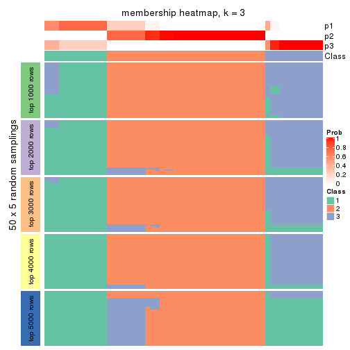
membership_heatmap(res, k = 4)
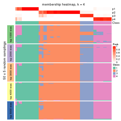
membership_heatmap(res, k = 5)
membership_heatmap(res, k = 6)
As soon as we have had the classes for columns, we can look for signatures which are significantly different between classes which can be candidate marks for certain classes. Following are the heatmaps for signatures.
Signature heatmaps where rows are scaled:
get_signatures(res, k = 2)
get_signatures(res, k = 3)
get_signatures(res, k = 4)
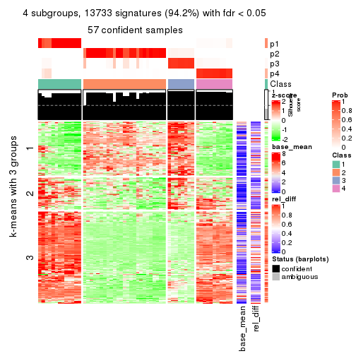
get_signatures(res, k = 5)
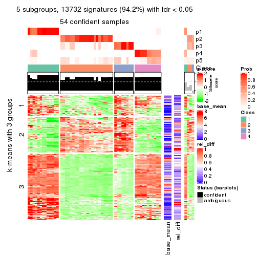
get_signatures(res, k = 6)
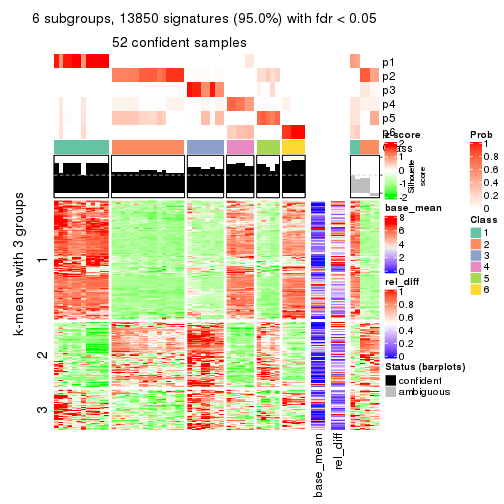
Signature heatmaps where rows are not scaled:
get_signatures(res, k = 2, scale_rows = FALSE)

get_signatures(res, k = 3, scale_rows = FALSE)
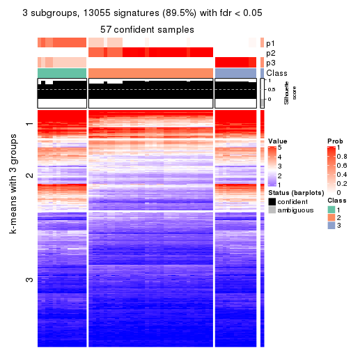
get_signatures(res, k = 4, scale_rows = FALSE)
get_signatures(res, k = 5, scale_rows = FALSE)
get_signatures(res, k = 6, scale_rows = FALSE)
Compare the overlap of signatures from different k:
compare_signatures(res)
get_signature() returns a data frame invisibly. TO get the list of signatures, the function
call should be assigned to a variable explicitly. In following code, if plot argument is set
to FALSE, no heatmap is plotted while only the differential analysis is performed.
# code only for demonstration
tb = get_signature(res, k = ..., plot = FALSE)
An example of the output of tb is:
#>   which_row         fdr    mean_1    mean_2 scaled_mean_1 scaled_mean_2 km
#> 1        38 0.042760348  8.373488  9.131774    -0.5533452     0.5164555  1
#> 2        40 0.018707592  7.106213  8.469186    -0.6173731     0.5762149  1
#> 3        55 0.019134737 10.221463 11.207825    -0.6159697     0.5749050  1
#> 4        59 0.006059896  5.921854  7.869574    -0.6899429     0.6439467  1
#> 5        60 0.018055526  8.928898 10.211722    -0.6204761     0.5791110  1
#> 6        98 0.009384629 15.714769 14.887706     0.6635654    -0.6193277  2
...
The columns in tb are:
which_row: row indices corresponding to the input matrix.fdr: FDR for the differential test. mean_x: The mean value in group x.scaled_mean_x: The mean value in group x after rows are scaled.km: Row groups if k-means clustering is applied to rows.UMAP plot which shows how samples are separated.
dimension_reduction(res, k = 2, method = "UMAP")

dimension_reduction(res, k = 3, method = "UMAP")
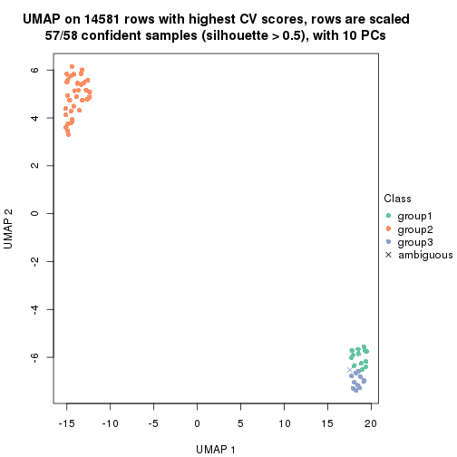
dimension_reduction(res, k = 4, method = "UMAP")
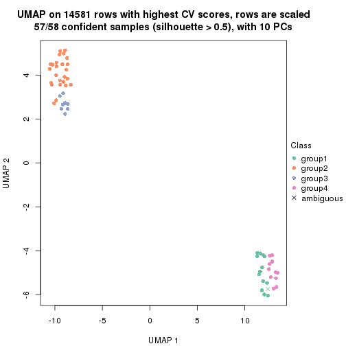
dimension_reduction(res, k = 5, method = "UMAP")
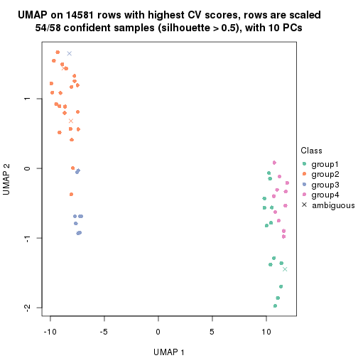
dimension_reduction(res, k = 6, method = "UMAP")
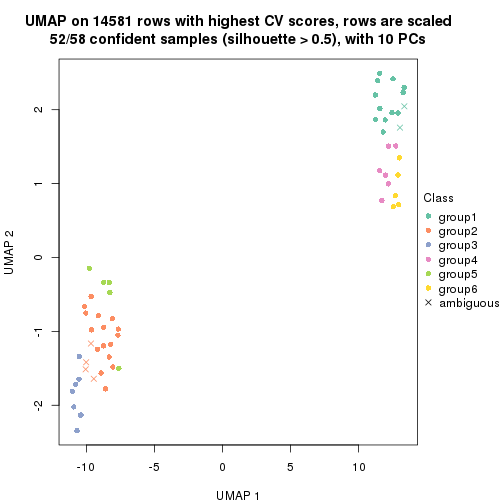
Following heatmap shows how subgroups are split when increasing k:
collect_classes(res)
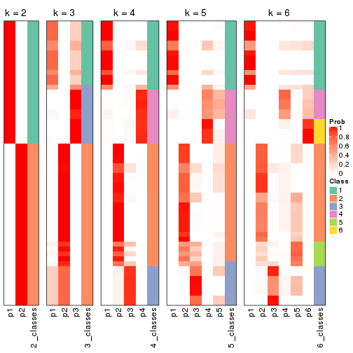
If matrix rows can be associated to genes, consider to use functional_enrichment(res,
...) to perform function enrichment for the signature genes. See this vignette for more detailed explanations.
The object with results only for a single top-value method and a single partition method can be extracted as:
res = res_list["CV", "pam"]
# you can also extract it by
# res = res_list["CV:pam"]
A summary of res and all the functions that can be applied to it:
res
#> A 'ConsensusPartition' object with k = 2, 3, 4, 5, 6.
#>   On a matrix with 14581 rows and 58 columns.
#>   Top rows (1000, 2000, 3000, 4000, 5000) are extracted by 'CV' method.
#>   Subgroups are detected by 'pam' method.
#>   Performed in total 1250 partitions by row resampling.
#>   Best k for subgroups seems to be 4.
#>
#> Following methods can be applied to this 'ConsensusPartition' object:
#>  [1] "cola_report"             "collect_classes"         "collect_plots"
#>  [4] "collect_stats"           "colnames"                "compare_signatures"
#>  [7] "consensus_heatmap"       "dimension_reduction"     "functional_enrichment"
#> [10] "get_anno_col"            "get_anno"                "get_classes"
#> [13] "get_consensus"           "get_matrix"              "get_membership"
#> [16] "get_param"               "get_signatures"          "get_stats"
#> [19] "is_best_k"               "is_stable_k"             "membership_heatmap"
#> [22] "ncol"                    "nrow"                    "plot_ecdf"
#> [25] "rownames"                "select_partition_number" "show"
#> [28] "suggest_best_k"          "test_to_known_factors"
collect_plots() function collects all the plots made from res for all k (number of partitions)
into one single page to provide an easy and fast comparison between different k.
collect_plots(res)
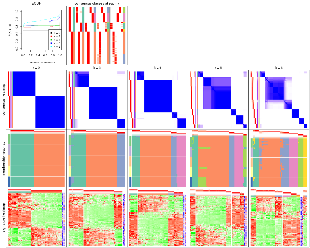
The plots are:
k and the heatmap of
predicted classes for each k.k.k.k.All the plots in panels can be made by individual functions and they are plotted later in this section.
select_partition_number() produces several plots showing different
statistics for choosing “optimized” k. There are following statistics:
k;k, the area increased is defined as \(A_k - A_{k-1}\).The detailed explanations of these statistics can be found in the cola vignette.
Generally speaking, lower PAC score, higher mean silhouette score or higher
concordance corresponds to better partition. Rand index and Jaccard index
measure how similar the current partition is compared to partition with k-1.
If they are too similar, we won't accept k is better than k-1.
select_partition_number(res)

The numeric values for all these statistics can be obtained by get_stats().
get_stats(res)
#>   k 1-PAC mean_silhouette concordance area_increased  Rand Jaccard
#> 2 2 1.000           1.000       1.000         0.4996 0.501   0.501
#> 3 3 1.000           0.974       0.987         0.1778 0.913   0.826
#> 4 4 1.000           0.993       0.995         0.0584 0.964   0.912
#> 5 5 0.848           0.901       0.926         0.0802 0.982   0.952
#> 6 6 0.890           0.866       0.943         0.1517 0.861   0.617
suggest_best_k() suggests the best \(k\) based on these statistics. The rules are as follows:
suggest_best_k(res)
#> [1] 4
#> attr(,"optional")
#> [1] 2 3
There is also optional best \(k\) = 2 3 that is worth to check.
Following shows the table of the partitions (You need to click the show/hide
code output link to see it). The membership matrix (columns with name p*)
is inferred by
clue::cl_consensus()
function with the SE method. Basically the value in the membership matrix
represents the probability to belong to a certain group. The finall class
label for an item is determined with the group with highest probability it
belongs to.
In get_classes() function, the entropy is calculated from the membership
matrix and the silhouette score is calculated from the consensus matrix.
cbind(get_classes(res, k = 2), get_membership(res, k = 2))
#>           class entropy silhouette p1 p2
#> ERR789082     2       0          1  0  1
#> ERR789083     2       0          1  0  1
#> ERR789191     2       0          1  0  1
#> ERR789192     2       0          1  0  1
#> ERR789213     1       0          1  1  0
#> ERR789385     1       0          1  1  0
#> ERR789393     1       0          1  1  0
#> ERR789394     1       0          1  1  0
#> ERR789193     2       0          1  0  1
#> ERR789194     2       0          1  0  1
#> ERR789195     2       0          1  0  1
#> ERR789196     2       0          1  0  1
#> ERR789388     1       0          1  1  0
#> ERR789197     2       0          1  0  1
#> ERR789198     2       0          1  0  1
#> ERR789214     1       0          1  1  0
#> ERR789397     1       0          1  1  0
#> ERR789398     1       0          1  1  0
#> ERR789199     2       0          1  0  1
#> ERR789200     2       0          1  0  1
#> ERR789201     2       0          1  0  1
#> ERR789202     2       0          1  0  1
#> ERR789215     1       0          1  1  0
#> ERR789203     2       0          1  0  1
#> ERR789204     2       0          1  0  1
#> ERR789383     1       0          1  1  0
#> ERR789205     2       0          1  0  1
#> ERR789206     2       0          1  0  1
#> ERR789399     1       0          1  1  0
#> ERR789400     1       0          1  1  0
#> ERR789207     2       0          1  0  1
#> ERR789208     2       0          1  0  1
#> ERR789209     2       0          1  0  1
#> ERR789210     2       0          1  0  1
#> ERR789211     2       0          1  0  1
#> ERR789212     2       0          1  0  1
#> ERR789386     1       0          1  1  0
#> ERR789076     2       0          1  0  1
#> ERR789077     2       0          1  0  1
#> ERR789384     1       0          1  1  0
#> ERR789078     2       0          1  0  1
#> ERR789079     2       0          1  0  1
#> ERR789216     1       0          1  1  0
#> ERR789080     2       0          1  0  1
#> ERR789387     1       0          1  1  0
#> ERR789081     2       0          1  0  1
#> ERR789064     2       0          1  0  1
#> ERR779485     2       0          1  0  1
#> ERR789065     2       0          1  0  1
#> ERR789401     1       0          1  1  0
#> ERR789402     1       0          1  1  0
#> ERR789403     1       0          1  1  0
#> ERR789389     1       0          1  1  0
#> ERR789395     1       0          1  1  0
#> ERR789396     1       0          1  1  0
#> ERR789390     1       0          1  1  0
#> ERR789391     1       0          1  1  0
#> ERR789392     1       0          1  1  0
cbind(get_classes(res, k = 3), get_membership(res, k = 3))
#>           class entropy silhouette    p1 p2    p3
#> ERR789082     2  0.0000      1.000 0.000  1 0.000
#> ERR789083     2  0.0000      1.000 0.000  1 0.000
#> ERR789191     2  0.0000      1.000 0.000  1 0.000
#> ERR789192     2  0.0000      1.000 0.000  1 0.000
#> ERR789213     1  0.0000      0.949 1.000  0 0.000
#> ERR789385     1  0.0000      0.949 1.000  0 0.000
#> ERR789393     1  0.0000      0.949 1.000  0 0.000
#> ERR789394     1  0.0000      0.949 1.000  0 0.000
#> ERR789193     2  0.0000      1.000 0.000  1 0.000
#> ERR789194     2  0.0000      1.000 0.000  1 0.000
#> ERR789195     2  0.0000      1.000 0.000  1 0.000
#> ERR789196     2  0.0000      1.000 0.000  1 0.000
#> ERR789388     1  0.0000      0.949 1.000  0 0.000
#> ERR789197     2  0.0000      1.000 0.000  1 0.000
#> ERR789198     2  0.0000      1.000 0.000  1 0.000
#> ERR789214     1  0.0000      0.949 1.000  0 0.000
#> ERR789397     1  0.0592      0.943 0.988  0 0.012
#> ERR789398     1  0.0747      0.941 0.984  0 0.016
#> ERR789199     2  0.0000      1.000 0.000  1 0.000
#> ERR789200     2  0.0000      1.000 0.000  1 0.000
#> ERR789201     2  0.0000      1.000 0.000  1 0.000
#> ERR789202     2  0.0000      1.000 0.000  1 0.000
#> ERR789215     1  0.5465      0.651 0.712  0 0.288
#> ERR789203     2  0.0000      1.000 0.000  1 0.000
#> ERR789204     2  0.0000      1.000 0.000  1 0.000
#> ERR789383     3  0.0000      1.000 0.000  0 1.000
#> ERR789205     2  0.0000      1.000 0.000  1 0.000
#> ERR789206     2  0.0000      1.000 0.000  1 0.000
#> ERR789399     3  0.0000      1.000 0.000  0 1.000
#> ERR789400     3  0.0000      1.000 0.000  0 1.000
#> ERR789207     2  0.0000      1.000 0.000  1 0.000
#> ERR789208     2  0.0000      1.000 0.000  1 0.000
#> ERR789209     2  0.0000      1.000 0.000  1 0.000
#> ERR789210     2  0.0000      1.000 0.000  1 0.000
#> ERR789211     2  0.0000      1.000 0.000  1 0.000
#> ERR789212     2  0.0000      1.000 0.000  1 0.000
#> ERR789386     1  0.0000      0.949 1.000  0 0.000
#> ERR789076     2  0.0000      1.000 0.000  1 0.000
#> ERR789077     2  0.0000      1.000 0.000  1 0.000
#> ERR789384     1  0.0000      0.949 1.000  0 0.000
#> ERR789078     2  0.0000      1.000 0.000  1 0.000
#> ERR789079     2  0.0000      1.000 0.000  1 0.000
#> ERR789216     1  0.0000      0.949 1.000  0 0.000
#> ERR789080     2  0.0000      1.000 0.000  1 0.000
#> ERR789387     3  0.0000      1.000 0.000  0 1.000
#> ERR789081     2  0.0000      1.000 0.000  1 0.000
#> ERR789064     2  0.0000      1.000 0.000  1 0.000
#> ERR779485     2  0.0000      1.000 0.000  1 0.000
#> ERR789065     2  0.0000      1.000 0.000  1 0.000
#> ERR789401     3  0.0000      1.000 0.000  0 1.000
#> ERR789402     3  0.0000      1.000 0.000  0 1.000
#> ERR789403     3  0.0000      1.000 0.000  0 1.000
#> ERR789389     1  0.0000      0.949 1.000  0 0.000
#> ERR789395     3  0.0000      1.000 0.000  0 1.000
#> ERR789396     3  0.0000      1.000 0.000  0 1.000
#> ERR789390     1  0.4702      0.763 0.788  0 0.212
#> ERR789391     1  0.4702      0.763 0.788  0 0.212
#> ERR789392     1  0.0000      0.949 1.000  0 0.000
cbind(get_classes(res, k = 4), get_membership(res, k = 4))
#>           class entropy silhouette    p1 p2    p3    p4
#> ERR789082     2  0.0000      1.000 0.000  1 0.000 0.000
#> ERR789083     2  0.0000      1.000 0.000  1 0.000 0.000
#> ERR789191     2  0.0000      1.000 0.000  1 0.000 0.000
#> ERR789192     2  0.0000      1.000 0.000  1 0.000 0.000
#> ERR789213     4  0.0000      0.984 0.000  0 0.000 1.000
#> ERR789385     4  0.0000      0.984 0.000  0 0.000 1.000
#> ERR789393     4  0.0000      0.984 0.000  0 0.000 1.000
#> ERR789394     4  0.0000      0.984 0.000  0 0.000 1.000
#> ERR789193     2  0.0000      1.000 0.000  1 0.000 0.000
#> ERR789194     2  0.0000      1.000 0.000  1 0.000 0.000
#> ERR789195     2  0.0000      1.000 0.000  1 0.000 0.000
#> ERR789196     2  0.0000      1.000 0.000  1 0.000 0.000
#> ERR789388     3  0.0592      0.993 0.000  0 0.984 0.016
#> ERR789197     2  0.0000      1.000 0.000  1 0.000 0.000
#> ERR789198     2  0.0000      1.000 0.000  1 0.000 0.000
#> ERR789214     3  0.0592      0.993 0.000  0 0.984 0.016
#> ERR789397     3  0.0592      0.993 0.000  0 0.984 0.016
#> ERR789398     3  0.0592      0.993 0.000  0 0.984 0.016
#> ERR789199     2  0.0000      1.000 0.000  1 0.000 0.000
#> ERR789200     2  0.0000      1.000 0.000  1 0.000 0.000
#> ERR789201     2  0.0000      1.000 0.000  1 0.000 0.000
#> ERR789202     2  0.0000      1.000 0.000  1 0.000 0.000
#> ERR789215     4  0.3224      0.843 0.120  0 0.016 0.864
#> ERR789203     2  0.0000      1.000 0.000  1 0.000 0.000
#> ERR789204     2  0.0000      1.000 0.000  1 0.000 0.000
#> ERR789383     1  0.0592      0.992 0.984  0 0.016 0.000
#> ERR789205     2  0.0000      1.000 0.000  1 0.000 0.000
#> ERR789206     2  0.0000      1.000 0.000  1 0.000 0.000
#> ERR789399     1  0.0592      0.992 0.984  0 0.016 0.000
#> ERR789400     1  0.0592      0.992 0.984  0 0.016 0.000
#> ERR789207     2  0.0000      1.000 0.000  1 0.000 0.000
#> ERR789208     2  0.0000      1.000 0.000  1 0.000 0.000
#> ERR789209     2  0.0000      1.000 0.000  1 0.000 0.000
#> ERR789210     2  0.0000      1.000 0.000  1 0.000 0.000
#> ERR789211     2  0.0000      1.000 0.000  1 0.000 0.000
#> ERR789212     2  0.0000      1.000 0.000  1 0.000 0.000
#> ERR789386     4  0.0000      0.984 0.000  0 0.000 1.000
#> ERR789076     2  0.0000      1.000 0.000  1 0.000 0.000
#> ERR789077     2  0.0000      1.000 0.000  1 0.000 0.000
#> ERR789384     4  0.0000      0.984 0.000  0 0.000 1.000
#> ERR789078     2  0.0000      1.000 0.000  1 0.000 0.000
#> ERR789079     2  0.0000      1.000 0.000  1 0.000 0.000
#> ERR789216     4  0.0000      0.984 0.000  0 0.000 1.000
#> ERR789080     2  0.0000      1.000 0.000  1 0.000 0.000
#> ERR789387     1  0.0000      0.992 1.000  0 0.000 0.000
#> ERR789081     2  0.0000      1.000 0.000  1 0.000 0.000
#> ERR789064     2  0.0000      1.000 0.000  1 0.000 0.000
#> ERR779485     2  0.0000      1.000 0.000  1 0.000 0.000
#> ERR789065     2  0.0000      1.000 0.000  1 0.000 0.000
#> ERR789401     1  0.0336      0.993 0.992  0 0.008 0.000
#> ERR789402     1  0.0000      0.992 1.000  0 0.000 0.000
#> ERR789403     1  0.0592      0.992 0.984  0 0.016 0.000
#> ERR789389     4  0.0000      0.984 0.000  0 0.000 1.000
#> ERR789395     1  0.0000      0.992 1.000  0 0.000 0.000
#> ERR789396     1  0.0000      0.992 1.000  0 0.000 0.000
#> ERR789390     3  0.0000      0.985 0.000  0 1.000 0.000
#> ERR789391     3  0.0000      0.985 0.000  0 1.000 0.000
#> ERR789392     4  0.0000      0.984 0.000  0 0.000 1.000
cbind(get_classes(res, k = 5), get_membership(res, k = 5))
#>           class entropy silhouette    p1    p2    p3    p4    p5
#> ERR789082     2  0.0000      0.915 0.000 1.000 0.000 0.000 0.000
#> ERR789083     2  0.0000      0.915 0.000 1.000 0.000 0.000 0.000
#> ERR789191     2  0.0000      0.915 0.000 1.000 0.000 0.000 0.000
#> ERR789192     2  0.0000      0.915 0.000 1.000 0.000 0.000 0.000
#> ERR789213     4  0.0000      1.000 0.000 0.000 0.000 1.000 0.000
#> ERR789385     4  0.0000      1.000 0.000 0.000 0.000 1.000 0.000
#> ERR789393     4  0.0000      1.000 0.000 0.000 0.000 1.000 0.000
#> ERR789394     4  0.0000      1.000 0.000 0.000 0.000 1.000 0.000
#> ERR789193     2  0.3774      0.762 0.296 0.704 0.000 0.000 0.000
#> ERR789194     2  0.3774      0.762 0.296 0.704 0.000 0.000 0.000
#> ERR789195     2  0.0162      0.914 0.004 0.996 0.000 0.000 0.000
#> ERR789196     2  0.0000      0.915 0.000 1.000 0.000 0.000 0.000
#> ERR789388     3  0.0000      0.996 0.000 0.000 1.000 0.000 0.000
#> ERR789197     2  0.0000      0.915 0.000 1.000 0.000 0.000 0.000
#> ERR789198     2  0.0000      0.915 0.000 1.000 0.000 0.000 0.000
#> ERR789214     3  0.0000      0.996 0.000 0.000 1.000 0.000 0.000
#> ERR789397     3  0.0000      0.996 0.000 0.000 1.000 0.000 0.000
#> ERR789398     3  0.0000      0.996 0.000 0.000 1.000 0.000 0.000
#> ERR789199     2  0.0000      0.915 0.000 1.000 0.000 0.000 0.000
#> ERR789200     2  0.0000      0.915 0.000 1.000 0.000 0.000 0.000
#> ERR789201     2  0.0404      0.912 0.012 0.988 0.000 0.000 0.000
#> ERR789202     2  0.1851      0.883 0.088 0.912 0.000 0.000 0.000
#> ERR789215     5  0.3210      0.617 0.000 0.000 0.000 0.212 0.788
#> ERR789203     2  0.3774      0.762 0.296 0.704 0.000 0.000 0.000
#> ERR789204     2  0.3774      0.762 0.296 0.704 0.000 0.000 0.000
#> ERR789383     5  0.0000      0.846 0.000 0.000 0.000 0.000 1.000
#> ERR789205     2  0.3774      0.762 0.296 0.704 0.000 0.000 0.000
#> ERR789206     2  0.3774      0.762 0.296 0.704 0.000 0.000 0.000
#> ERR789399     5  0.0000      0.846 0.000 0.000 0.000 0.000 1.000
#> ERR789400     5  0.0000      0.846 0.000 0.000 0.000 0.000 1.000
#> ERR789207     2  0.0000      0.915 0.000 1.000 0.000 0.000 0.000
#> ERR789208     2  0.0000      0.915 0.000 1.000 0.000 0.000 0.000
#> ERR789209     2  0.0000      0.915 0.000 1.000 0.000 0.000 0.000
#> ERR789210     2  0.0000      0.915 0.000 1.000 0.000 0.000 0.000
#> ERR789211     2  0.0000      0.915 0.000 1.000 0.000 0.000 0.000
#> ERR789212     2  0.0000      0.915 0.000 1.000 0.000 0.000 0.000
#> ERR789386     4  0.0000      1.000 0.000 0.000 0.000 1.000 0.000
#> ERR789076     2  0.1043      0.903 0.040 0.960 0.000 0.000 0.000
#> ERR789077     2  0.0000      0.915 0.000 1.000 0.000 0.000 0.000
#> ERR789384     4  0.0000      1.000 0.000 0.000 0.000 1.000 0.000
#> ERR789078     2  0.0880      0.906 0.032 0.968 0.000 0.000 0.000
#> ERR789079     2  0.0000      0.915 0.000 1.000 0.000 0.000 0.000
#> ERR789216     4  0.0000      1.000 0.000 0.000 0.000 1.000 0.000
#> ERR789080     2  0.1121      0.902 0.044 0.956 0.000 0.000 0.000
#> ERR789387     1  0.3774      0.930 0.704 0.000 0.000 0.000 0.296
#> ERR789081     2  0.0000      0.915 0.000 1.000 0.000 0.000 0.000
#> ERR789064     2  0.3395      0.798 0.236 0.764 0.000 0.000 0.000
#> ERR779485     2  0.3774      0.762 0.296 0.704 0.000 0.000 0.000
#> ERR789065     2  0.3774      0.762 0.296 0.704 0.000 0.000 0.000
#> ERR789401     1  0.4171      0.856 0.604 0.000 0.000 0.000 0.396
#> ERR789402     1  0.3774      0.930 0.704 0.000 0.000 0.000 0.296
#> ERR789403     1  0.4273      0.781 0.552 0.000 0.000 0.000 0.448
#> ERR789389     4  0.0000      1.000 0.000 0.000 0.000 1.000 0.000
#> ERR789395     1  0.3774      0.930 0.704 0.000 0.000 0.000 0.296
#> ERR789396     1  0.3774      0.930 0.704 0.000 0.000 0.000 0.296
#> ERR789390     3  0.0162      0.994 0.000 0.000 0.996 0.000 0.004
#> ERR789391     3  0.0510      0.985 0.000 0.000 0.984 0.000 0.016
#> ERR789392     4  0.0000      1.000 0.000 0.000 0.000 1.000 0.000
cbind(get_classes(res, k = 6), get_membership(res, k = 6))
#>           class entropy silhouette    p1    p2    p3 p4    p5    p6
#> ERR789082     2  0.0146     0.9165 0.000 0.996 0.004  0 0.000 0.000
#> ERR789083     2  0.0000     0.9167 0.000 1.000 0.000  0 0.000 0.000
#> ERR789191     2  0.0000     0.9167 0.000 1.000 0.000  0 0.000 0.000
#> ERR789192     2  0.0260     0.9156 0.000 0.992 0.008  0 0.000 0.000
#> ERR789213     4  0.0000     1.0000 0.000 0.000 0.000  1 0.000 0.000
#> ERR789385     4  0.0000     1.0000 0.000 0.000 0.000  1 0.000 0.000
#> ERR789393     4  0.0000     1.0000 0.000 0.000 0.000  1 0.000 0.000
#> ERR789394     4  0.0000     1.0000 0.000 0.000 0.000  1 0.000 0.000
#> ERR789193     3  0.3126     0.6668 0.000 0.248 0.752  0 0.000 0.000
#> ERR789194     3  0.1863     0.7552 0.000 0.104 0.896  0 0.000 0.000
#> ERR789195     2  0.1610     0.8775 0.000 0.916 0.084  0 0.000 0.000
#> ERR789196     2  0.2003     0.8445 0.000 0.884 0.116  0 0.000 0.000
#> ERR789388     5  0.0000     0.9959 0.000 0.000 0.000  0 1.000 0.000
#> ERR789197     2  0.0937     0.9048 0.000 0.960 0.040  0 0.000 0.000
#> ERR789198     2  0.0937     0.9048 0.000 0.960 0.040  0 0.000 0.000
#> ERR789214     5  0.0000     0.9959 0.000 0.000 0.000  0 1.000 0.000
#> ERR789397     5  0.0000     0.9959 0.000 0.000 0.000  0 1.000 0.000
#> ERR789398     5  0.0000     0.9959 0.000 0.000 0.000  0 1.000 0.000
#> ERR789199     2  0.0937     0.9048 0.000 0.960 0.040  0 0.000 0.000
#> ERR789200     2  0.0937     0.9048 0.000 0.960 0.040  0 0.000 0.000
#> ERR789201     2  0.3266     0.6226 0.000 0.728 0.272  0 0.000 0.000
#> ERR789202     3  0.3857     0.0922 0.000 0.468 0.532  0 0.000 0.000
#> ERR789215     6  0.0000     1.0000 0.000 0.000 0.000  0 0.000 1.000
#> ERR789203     3  0.0363     0.7866 0.000 0.012 0.988  0 0.000 0.000
#> ERR789204     3  0.0547     0.7926 0.000 0.020 0.980  0 0.000 0.000
#> ERR789383     6  0.0000     1.0000 0.000 0.000 0.000  0 0.000 1.000
#> ERR789205     3  0.0547     0.7919 0.000 0.020 0.980  0 0.000 0.000
#> ERR789206     3  0.0632     0.7931 0.000 0.024 0.976  0 0.000 0.000
#> ERR789399     6  0.0000     1.0000 0.000 0.000 0.000  0 0.000 1.000
#> ERR789400     6  0.0000     1.0000 0.000 0.000 0.000  0 0.000 1.000
#> ERR789207     2  0.0260     0.9157 0.000 0.992 0.008  0 0.000 0.000
#> ERR789208     2  0.0260     0.9157 0.000 0.992 0.008  0 0.000 0.000
#> ERR789209     2  0.0260     0.9157 0.000 0.992 0.008  0 0.000 0.000
#> ERR789210     2  0.0260     0.9157 0.000 0.992 0.008  0 0.000 0.000
#> ERR789211     2  0.0260     0.9157 0.000 0.992 0.008  0 0.000 0.000
#> ERR789212     2  0.0260     0.9157 0.000 0.992 0.008  0 0.000 0.000
#> ERR789386     4  0.0000     1.0000 0.000 0.000 0.000  1 0.000 0.000
#> ERR789076     2  0.3531     0.4467 0.000 0.672 0.328  0 0.000 0.000
#> ERR789077     2  0.0146     0.9165 0.000 0.996 0.004  0 0.000 0.000
#> ERR789384     4  0.0000     1.0000 0.000 0.000 0.000  1 0.000 0.000
#> ERR789078     2  0.2597     0.7338 0.000 0.824 0.176  0 0.000 0.000
#> ERR789079     2  0.0000     0.9167 0.000 1.000 0.000  0 0.000 0.000
#> ERR789216     4  0.0000     1.0000 0.000 0.000 0.000  1 0.000 0.000
#> ERR789080     2  0.3620     0.3850 0.000 0.648 0.352  0 0.000 0.000
#> ERR789387     1  0.0000     0.9253 1.000 0.000 0.000  0 0.000 0.000
#> ERR789081     2  0.0000     0.9167 0.000 1.000 0.000  0 0.000 0.000
#> ERR789064     3  0.3838     0.2754 0.000 0.448 0.552  0 0.000 0.000
#> ERR779485     3  0.0458     0.7903 0.000 0.016 0.984  0 0.000 0.000
#> ERR789065     3  0.0713     0.7833 0.000 0.028 0.972  0 0.000 0.000
#> ERR789401     1  0.2631     0.8147 0.820 0.000 0.000  0 0.000 0.180
#> ERR789402     1  0.0000     0.9253 1.000 0.000 0.000  0 0.000 0.000
#> ERR789403     1  0.2697     0.8058 0.812 0.000 0.000  0 0.000 0.188
#> ERR789389     4  0.0000     1.0000 0.000 0.000 0.000  1 0.000 0.000
#> ERR789395     1  0.0000     0.9253 1.000 0.000 0.000  0 0.000 0.000
#> ERR789396     1  0.0000     0.9253 1.000 0.000 0.000  0 0.000 0.000
#> ERR789390     5  0.0146     0.9940 0.000 0.000 0.000  0 0.996 0.004
#> ERR789391     5  0.0458     0.9845 0.000 0.000 0.000  0 0.984 0.016
#> ERR789392     4  0.0000     1.0000 0.000 0.000 0.000  1 0.000 0.000
Heatmaps for the consensus matrix. It visualizes the probability of two samples to be in a same group.
consensus_heatmap(res, k = 2)

consensus_heatmap(res, k = 3)
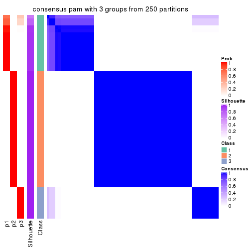
consensus_heatmap(res, k = 4)
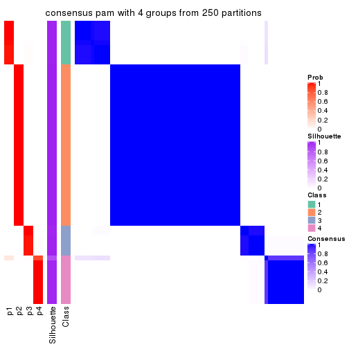
consensus_heatmap(res, k = 5)
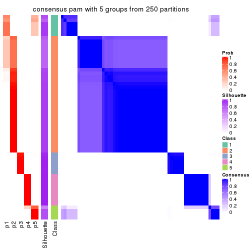
consensus_heatmap(res, k = 6)
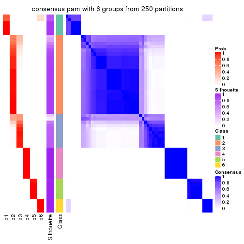
Heatmaps for the membership of samples in all partitions to see how consistent they are:
membership_heatmap(res, k = 2)

membership_heatmap(res, k = 3)
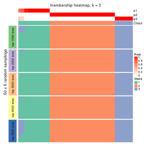
membership_heatmap(res, k = 4)
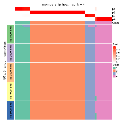
membership_heatmap(res, k = 5)
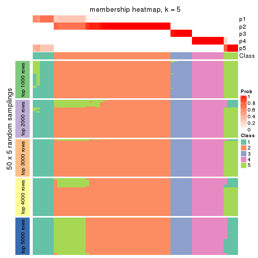
membership_heatmap(res, k = 6)
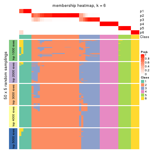
As soon as we have had the classes for columns, we can look for signatures which are significantly different between classes which can be candidate marks for certain classes. Following are the heatmaps for signatures.
Signature heatmaps where rows are scaled:
get_signatures(res, k = 2)

get_signatures(res, k = 3)
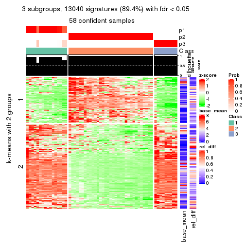
get_signatures(res, k = 4)
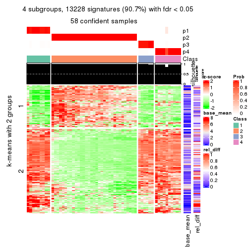
get_signatures(res, k = 5)
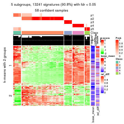
get_signatures(res, k = 6)
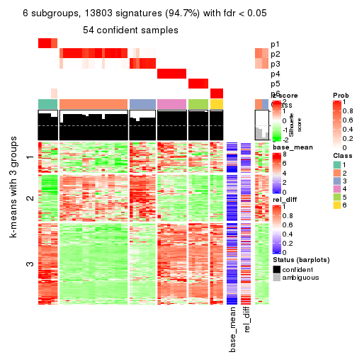
Signature heatmaps where rows are not scaled:
get_signatures(res, k = 2, scale_rows = FALSE)

get_signatures(res, k = 3, scale_rows = FALSE)
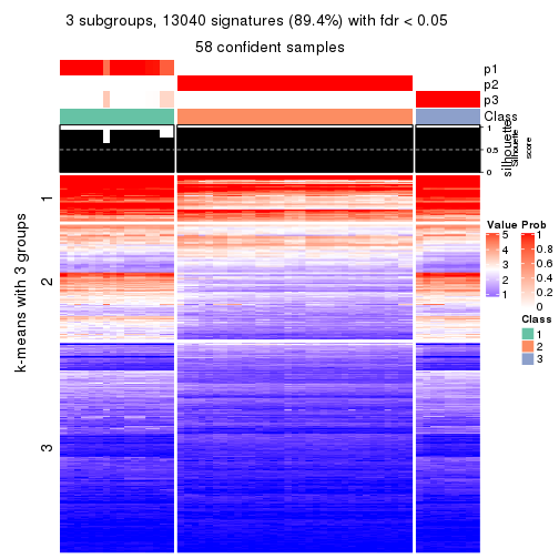
get_signatures(res, k = 4, scale_rows = FALSE)
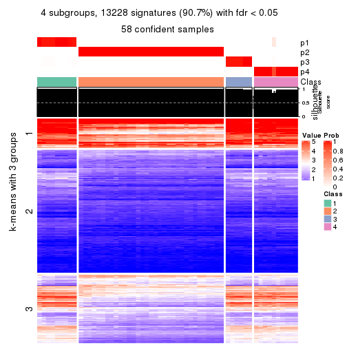
get_signatures(res, k = 5, scale_rows = FALSE)
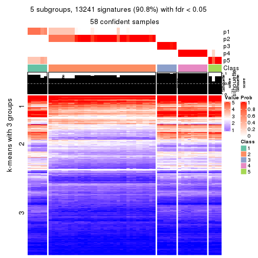
get_signatures(res, k = 6, scale_rows = FALSE)
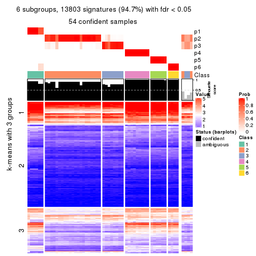
Compare the overlap of signatures from different k:
compare_signatures(res)
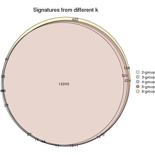
get_signature() returns a data frame invisibly. TO get the list of signatures, the function
call should be assigned to a variable explicitly. In following code, if plot argument is set
to FALSE, no heatmap is plotted while only the differential analysis is performed.
# code only for demonstration
tb = get_signature(res, k = ..., plot = FALSE)
An example of the output of tb is:
#>   which_row         fdr    mean_1    mean_2 scaled_mean_1 scaled_mean_2 km
#> 1        38 0.042760348  8.373488  9.131774    -0.5533452     0.5164555  1
#> 2        40 0.018707592  7.106213  8.469186    -0.6173731     0.5762149  1
#> 3        55 0.019134737 10.221463 11.207825    -0.6159697     0.5749050  1
#> 4        59 0.006059896  5.921854  7.869574    -0.6899429     0.6439467  1
#> 5        60 0.018055526  8.928898 10.211722    -0.6204761     0.5791110  1
#> 6        98 0.009384629 15.714769 14.887706     0.6635654    -0.6193277  2
...
The columns in tb are:
which_row: row indices corresponding to the input matrix.fdr: FDR for the differential test. mean_x: The mean value in group x.scaled_mean_x: The mean value in group x after rows are scaled.km: Row groups if k-means clustering is applied to rows.UMAP plot which shows how samples are separated.
dimension_reduction(res, k = 2, method = "UMAP")

dimension_reduction(res, k = 3, method = "UMAP")
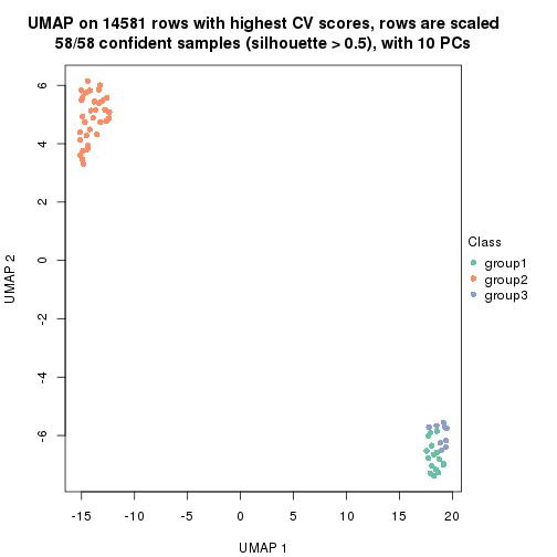
dimension_reduction(res, k = 4, method = "UMAP")
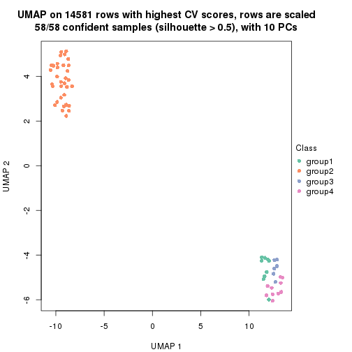
dimension_reduction(res, k = 5, method = "UMAP")
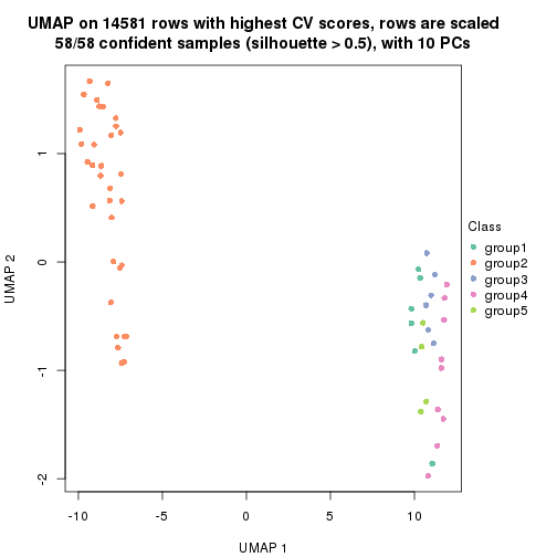
dimension_reduction(res, k = 6, method = "UMAP")
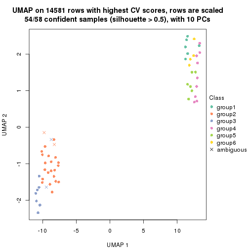
Following heatmap shows how subgroups are split when increasing k:
collect_classes(res)
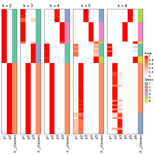
If matrix rows can be associated to genes, consider to use functional_enrichment(res,
...) to perform function enrichment for the signature genes. See this vignette for more detailed explanations.
The object with results only for a single top-value method and a single partition method can be extracted as:
res = res_list["CV", "mclust"]
# you can also extract it by
# res = res_list["CV:mclust"]
A summary of res and all the functions that can be applied to it:
res
#> A 'ConsensusPartition' object with k = 2, 3, 4, 5, 6.
#>   On a matrix with 14581 rows and 58 columns.
#>   Top rows (1000, 2000, 3000, 4000, 5000) are extracted by 'CV' method.
#>   Subgroups are detected by 'mclust' method.
#>   Performed in total 1250 partitions by row resampling.
#>   Best k for subgroups seems to be 2.
#>
#> Following methods can be applied to this 'ConsensusPartition' object:
#>  [1] "cola_report"             "collect_classes"         "collect_plots"
#>  [4] "collect_stats"           "colnames"                "compare_signatures"
#>  [7] "consensus_heatmap"       "dimension_reduction"     "functional_enrichment"
#> [10] "get_anno_col"            "get_anno"                "get_classes"
#> [13] "get_consensus"           "get_matrix"              "get_membership"
#> [16] "get_param"               "get_signatures"          "get_stats"
#> [19] "is_best_k"               "is_stable_k"             "membership_heatmap"
#> [22] "ncol"                    "nrow"                    "plot_ecdf"
#> [25] "rownames"                "select_partition_number" "show"
#> [28] "suggest_best_k"          "test_to_known_factors"
collect_plots() function collects all the plots made from res for all k (number of partitions)
into one single page to provide an easy and fast comparison between different k.
collect_plots(res)
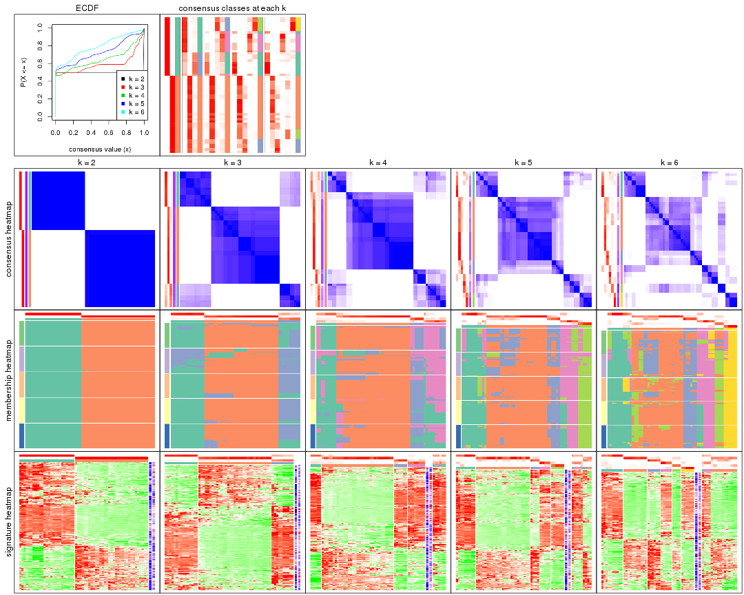
The plots are:
k and the heatmap of
predicted classes for each k.k.k.k.All the plots in panels can be made by individual functions and they are plotted later in this section.
select_partition_number() produces several plots showing different
statistics for choosing “optimized” k. There are following statistics:
k;k, the area increased is defined as \(A_k - A_{k-1}\).The detailed explanations of these statistics can be found in the cola vignette.
Generally speaking, lower PAC score, higher mean silhouette score or higher
concordance corresponds to better partition. Rand index and Jaccard index
measure how similar the current partition is compared to partition with k-1.
If they are too similar, we won't accept k is better than k-1.
select_partition_number(res)
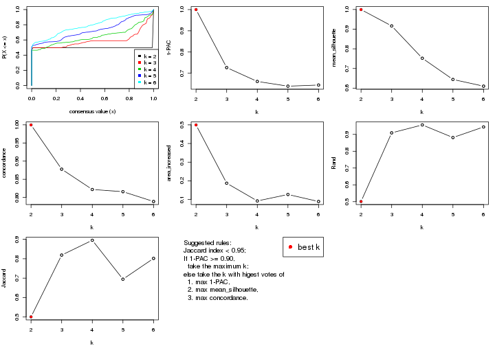
The numeric values for all these statistics can be obtained by get_stats().
get_stats(res)
#>   k 1-PAC mean_silhouette concordance area_increased  Rand Jaccard
#> 2 2 1.000           0.999       1.000         0.4996 0.501   0.501
#> 3 3 0.727           0.916       0.878         0.1873 0.909   0.819
#> 4 4 0.661           0.752       0.822         0.0923 0.956   0.895
#> 5 5 0.639           0.644       0.816         0.1268 0.881   0.695
#> 6 6 0.644           0.610       0.789         0.0892 0.944   0.802
suggest_best_k() suggests the best \(k\) based on these statistics. The rules are as follows:
suggest_best_k(res)
#> [1] 2
Following shows the table of the partitions (You need to click the show/hide
code output link to see it). The membership matrix (columns with name p*)
is inferred by
clue::cl_consensus()
function with the SE method. Basically the value in the membership matrix
represents the probability to belong to a certain group. The finall class
label for an item is determined with the group with highest probability it
belongs to.
In get_classes() function, the entropy is calculated from the membership
matrix and the silhouette score is calculated from the consensus matrix.
cbind(get_classes(res, k = 2), get_membership(res, k = 2))
#>           class entropy silhouette    p1    p2
#> ERR789082     2  0.0000      0.999 0.000 1.000
#> ERR789083     2  0.0000      0.999 0.000 1.000
#> ERR789191     2  0.0000      0.999 0.000 1.000
#> ERR789192     2  0.0000      0.999 0.000 1.000
#> ERR789213     1  0.0000      1.000 1.000 0.000
#> ERR789385     1  0.0000      1.000 1.000 0.000
#> ERR789393     1  0.0000      1.000 1.000 0.000
#> ERR789394     1  0.0000      1.000 1.000 0.000
#> ERR789193     2  0.0000      0.999 0.000 1.000
#> ERR789194     2  0.0000      0.999 0.000 1.000
#> ERR789195     2  0.0000      0.999 0.000 1.000
#> ERR789196     2  0.0000      0.999 0.000 1.000
#> ERR789388     1  0.0000      1.000 1.000 0.000
#> ERR789197     2  0.0000      0.999 0.000 1.000
#> ERR789198     2  0.0000      0.999 0.000 1.000
#> ERR789214     1  0.0000      1.000 1.000 0.000
#> ERR789397     1  0.0000      1.000 1.000 0.000
#> ERR789398     1  0.0000      1.000 1.000 0.000
#> ERR789199     2  0.0000      0.999 0.000 1.000
#> ERR789200     2  0.0000      0.999 0.000 1.000
#> ERR789201     2  0.0000      0.999 0.000 1.000
#> ERR789202     2  0.0000      0.999 0.000 1.000
#> ERR789215     1  0.0000      1.000 1.000 0.000
#> ERR789203     2  0.0000      0.999 0.000 1.000
#> ERR789204     2  0.0000      0.999 0.000 1.000
#> ERR789383     1  0.0000      1.000 1.000 0.000
#> ERR789205     2  0.0000      0.999 0.000 1.000
#> ERR789206     2  0.0000      0.999 0.000 1.000
#> ERR789399     1  0.0000      1.000 1.000 0.000
#> ERR789400     1  0.0000      1.000 1.000 0.000
#> ERR789207     2  0.0000      0.999 0.000 1.000
#> ERR789208     2  0.0000      0.999 0.000 1.000
#> ERR789209     2  0.0000      0.999 0.000 1.000
#> ERR789210     2  0.0000      0.999 0.000 1.000
#> ERR789211     2  0.0000      0.999 0.000 1.000
#> ERR789212     2  0.0000      0.999 0.000 1.000
#> ERR789386     1  0.0000      1.000 1.000 0.000
#> ERR789076     2  0.0000      0.999 0.000 1.000
#> ERR789077     2  0.0000      0.999 0.000 1.000
#> ERR789384     1  0.0000      1.000 1.000 0.000
#> ERR789078     2  0.0000      0.999 0.000 1.000
#> ERR789079     2  0.0000      0.999 0.000 1.000
#> ERR789216     1  0.0000      1.000 1.000 0.000
#> ERR789080     2  0.0672      0.992 0.008 0.992
#> ERR789387     1  0.0000      1.000 1.000 0.000
#> ERR789081     2  0.0000      0.999 0.000 1.000
#> ERR789064     2  0.0000      0.999 0.000 1.000
#> ERR779485     2  0.0672      0.992 0.008 0.992
#> ERR789065     2  0.0000      0.999 0.000 1.000
#> ERR789401     1  0.0000      1.000 1.000 0.000
#> ERR789402     1  0.0000      1.000 1.000 0.000
#> ERR789403     1  0.0000      1.000 1.000 0.000
#> ERR789389     1  0.0000      1.000 1.000 0.000
#> ERR789395     1  0.0000      1.000 1.000 0.000
#> ERR789396     1  0.0000      1.000 1.000 0.000
#> ERR789390     1  0.0000      1.000 1.000 0.000
#> ERR789391     1  0.0000      1.000 1.000 0.000
#> ERR789392     1  0.0000      1.000 1.000 0.000
cbind(get_classes(res, k = 3), get_membership(res, k = 3))
#>           class entropy silhouette    p1    p2    p3
#> ERR789082     2  0.0747      0.946 0.000 0.984 0.016
#> ERR789083     2  0.0747      0.946 0.000 0.984 0.016
#> ERR789191     2  0.0747      0.946 0.000 0.984 0.016
#> ERR789192     2  0.0747      0.946 0.000 0.984 0.016
#> ERR789213     1  0.2066      0.931 0.940 0.000 0.060
#> ERR789385     1  0.2066      0.931 0.940 0.000 0.060
#> ERR789393     1  0.1031      0.923 0.976 0.000 0.024
#> ERR789394     1  0.1031      0.923 0.976 0.000 0.024
#> ERR789193     2  0.4062      0.893 0.000 0.836 0.164
#> ERR789194     2  0.4062      0.893 0.000 0.836 0.164
#> ERR789195     2  0.1529      0.939 0.000 0.960 0.040
#> ERR789196     2  0.1529      0.939 0.000 0.960 0.040
#> ERR789388     1  0.2448      0.927 0.924 0.000 0.076
#> ERR789197     2  0.1529      0.939 0.000 0.960 0.040
#> ERR789198     2  0.1529      0.939 0.000 0.960 0.040
#> ERR789214     1  0.2448      0.927 0.924 0.000 0.076
#> ERR789397     1  0.1643      0.927 0.956 0.000 0.044
#> ERR789398     1  0.1643      0.927 0.956 0.000 0.044
#> ERR789199     2  0.1529      0.939 0.000 0.960 0.040
#> ERR789200     2  0.1529      0.939 0.000 0.960 0.040
#> ERR789201     2  0.0592      0.945 0.000 0.988 0.012
#> ERR789202     2  0.0592      0.945 0.000 0.988 0.012
#> ERR789215     1  0.2537      0.918 0.920 0.000 0.080
#> ERR789203     2  0.3192      0.925 0.000 0.888 0.112
#> ERR789204     2  0.3192      0.925 0.000 0.888 0.112
#> ERR789383     3  0.6180      0.806 0.416 0.000 0.584
#> ERR789205     2  0.2959      0.928 0.000 0.900 0.100
#> ERR789206     2  0.2959      0.928 0.000 0.900 0.100
#> ERR789399     3  0.5988      0.863 0.368 0.000 0.632
#> ERR789400     3  0.5968      0.865 0.364 0.000 0.636
#> ERR789207     2  0.0747      0.946 0.000 0.984 0.016
#> ERR789208     2  0.0747      0.946 0.000 0.984 0.016
#> ERR789209     2  0.0747      0.946 0.000 0.984 0.016
#> ERR789210     2  0.0747      0.946 0.000 0.984 0.016
#> ERR789211     2  0.0747      0.946 0.000 0.984 0.016
#> ERR789212     2  0.0747      0.946 0.000 0.984 0.016
#> ERR789386     1  0.1860      0.934 0.948 0.000 0.052
#> ERR789076     2  0.2711      0.929 0.000 0.912 0.088
#> ERR789077     2  0.0747      0.946 0.000 0.984 0.016
#> ERR789384     1  0.1860      0.934 0.948 0.000 0.052
#> ERR789078     2  0.2711      0.929 0.000 0.912 0.088
#> ERR789079     2  0.0747      0.946 0.000 0.984 0.016
#> ERR789216     1  0.1860      0.934 0.948 0.000 0.052
#> ERR789080     2  0.4235      0.887 0.000 0.824 0.176
#> ERR789387     3  0.6192      0.805 0.420 0.000 0.580
#> ERR789081     2  0.4121      0.892 0.000 0.832 0.168
#> ERR789064     2  0.2959      0.928 0.000 0.900 0.100
#> ERR779485     2  0.4555      0.874 0.000 0.800 0.200
#> ERR789065     2  0.4235      0.892 0.000 0.824 0.176
#> ERR789401     3  0.5216      0.882 0.260 0.000 0.740
#> ERR789402     3  0.5254      0.883 0.264 0.000 0.736
#> ERR789403     3  0.5216      0.882 0.260 0.000 0.740
#> ERR789389     3  0.6204      0.788 0.424 0.000 0.576
#> ERR789395     3  0.5254      0.883 0.264 0.000 0.736
#> ERR789396     3  0.5254      0.883 0.264 0.000 0.736
#> ERR789390     1  0.1860      0.928 0.948 0.000 0.052
#> ERR789391     1  0.1860      0.928 0.948 0.000 0.052
#> ERR789392     1  0.1031      0.923 0.976 0.000 0.024
cbind(get_classes(res, k = 4), get_membership(res, k = 4))
#>           class entropy silhouette    p1    p2    p3    p4
#> ERR789082     2  0.0592      0.905 0.000 0.984 0.016 0.000
#> ERR789083     2  0.0592      0.905 0.000 0.984 0.016 0.000
#> ERR789191     2  0.0592      0.905 0.000 0.984 0.016 0.000
#> ERR789192     2  0.0592      0.905 0.000 0.984 0.016 0.000
#> ERR789213     4  0.2216      0.648 0.000 0.000 0.092 0.908
#> ERR789385     4  0.2546      0.648 0.008 0.000 0.092 0.900
#> ERR789393     4  0.4304      0.543 0.000 0.000 0.284 0.716
#> ERR789394     4  0.4304      0.543 0.000 0.000 0.284 0.716
#> ERR789193     2  0.7317      0.539 0.284 0.560 0.012 0.144
#> ERR789194     2  0.7317      0.539 0.284 0.560 0.012 0.144
#> ERR789195     2  0.1975      0.897 0.016 0.936 0.048 0.000
#> ERR789196     2  0.1975      0.897 0.016 0.936 0.048 0.000
#> ERR789388     3  0.4188      0.723 0.004 0.000 0.752 0.244
#> ERR789197     2  0.1975      0.897 0.016 0.936 0.048 0.000
#> ERR789198     2  0.1975      0.897 0.016 0.936 0.048 0.000
#> ERR789214     3  0.4560      0.656 0.004 0.000 0.700 0.296
#> ERR789397     3  0.2053      0.869 0.004 0.000 0.924 0.072
#> ERR789398     3  0.2053      0.869 0.004 0.000 0.924 0.072
#> ERR789199     2  0.1975      0.897 0.016 0.936 0.048 0.000
#> ERR789200     2  0.1975      0.897 0.016 0.936 0.048 0.000
#> ERR789201     2  0.1114      0.905 0.016 0.972 0.008 0.004
#> ERR789202     2  0.1114      0.905 0.016 0.972 0.008 0.004
#> ERR789215     4  0.6364      0.496 0.144 0.000 0.204 0.652
#> ERR789203     2  0.4145      0.874 0.048 0.844 0.016 0.092
#> ERR789204     2  0.4145      0.874 0.048 0.844 0.016 0.092
#> ERR789383     1  0.6980      0.448 0.484 0.000 0.116 0.400
#> ERR789205     2  0.3996      0.876 0.044 0.852 0.016 0.088
#> ERR789206     2  0.3996      0.876 0.044 0.852 0.016 0.088
#> ERR789399     1  0.6783      0.484 0.512 0.000 0.100 0.388
#> ERR789400     1  0.6783      0.484 0.512 0.000 0.100 0.388
#> ERR789207     2  0.0592      0.905 0.000 0.984 0.016 0.000
#> ERR789208     2  0.0592      0.905 0.000 0.984 0.016 0.000
#> ERR789209     2  0.0779      0.905 0.000 0.980 0.016 0.004
#> ERR789210     2  0.0779      0.905 0.000 0.980 0.016 0.004
#> ERR789211     2  0.0592      0.905 0.000 0.984 0.016 0.000
#> ERR789212     2  0.0592      0.905 0.000 0.984 0.016 0.000
#> ERR789386     4  0.5540      0.597 0.108 0.000 0.164 0.728
#> ERR789076     2  0.3571      0.879 0.036 0.868 0.008 0.088
#> ERR789077     2  0.0592      0.905 0.000 0.984 0.016 0.000
#> ERR789384     4  0.5705      0.593 0.108 0.000 0.180 0.712
#> ERR789078     2  0.3237      0.887 0.040 0.888 0.008 0.064
#> ERR789079     2  0.0592      0.905 0.000 0.984 0.016 0.000
#> ERR789216     4  0.5569      0.600 0.104 0.000 0.172 0.724
#> ERR789080     2  0.4807      0.846 0.104 0.800 0.008 0.088
#> ERR789387     1  0.7009      0.450 0.488 0.000 0.120 0.392
#> ERR789081     2  0.4748      0.846 0.100 0.804 0.008 0.088
#> ERR789064     2  0.3498      0.886 0.044 0.880 0.016 0.060
#> ERR779485     2  0.7697      0.514 0.328 0.508 0.020 0.144
#> ERR789065     2  0.5113      0.842 0.104 0.788 0.016 0.092
#> ERR789401     1  0.5423      0.756 0.740 0.000 0.116 0.144
#> ERR789402     1  0.5291      0.768 0.740 0.000 0.080 0.180
#> ERR789403     1  0.5423      0.756 0.740 0.000 0.116 0.144
#> ERR789389     4  0.6395     -0.445 0.464 0.000 0.064 0.472
#> ERR789395     1  0.5291      0.768 0.740 0.000 0.080 0.180
#> ERR789396     1  0.5291      0.768 0.740 0.000 0.080 0.180
#> ERR789390     3  0.2198      0.870 0.008 0.000 0.920 0.072
#> ERR789391     3  0.2198      0.870 0.008 0.000 0.920 0.072
#> ERR789392     4  0.4304      0.543 0.000 0.000 0.284 0.716
cbind(get_classes(res, k = 5), get_membership(res, k = 5))
#>           class entropy silhouette    p1    p2    p3    p4    p5
#> ERR789082     2  0.0510      0.784 0.000 0.984 0.016 0.000 0.000
#> ERR789083     2  0.0290      0.783 0.000 0.992 0.008 0.000 0.000
#> ERR789191     2  0.0771      0.783 0.000 0.976 0.020 0.004 0.000
#> ERR789192     2  0.0771      0.783 0.000 0.976 0.020 0.004 0.000
#> ERR789213     4  0.0693      0.622 0.008 0.000 0.000 0.980 0.012
#> ERR789385     4  0.0671      0.621 0.004 0.000 0.000 0.980 0.016
#> ERR789393     4  0.3300      0.559 0.004 0.000 0.000 0.792 0.204
#> ERR789394     4  0.3300      0.559 0.004 0.000 0.000 0.792 0.204
#> ERR789193     3  0.3700      0.697 0.000 0.240 0.752 0.000 0.008
#> ERR789194     3  0.3700      0.697 0.000 0.240 0.752 0.000 0.008
#> ERR789195     2  0.3919      0.702 0.000 0.776 0.188 0.000 0.036
#> ERR789196     2  0.3919      0.702 0.000 0.776 0.188 0.000 0.036
#> ERR789388     5  0.3366      0.744 0.000 0.000 0.000 0.232 0.768
#> ERR789197     2  0.4394      0.655 0.000 0.732 0.228 0.004 0.036
#> ERR789198     2  0.4365      0.659 0.000 0.736 0.224 0.004 0.036
#> ERR789214     5  0.3661      0.710 0.000 0.000 0.000 0.276 0.724
#> ERR789397     5  0.1197      0.872 0.000 0.000 0.000 0.048 0.952
#> ERR789398     5  0.1197      0.872 0.000 0.000 0.000 0.048 0.952
#> ERR789199     2  0.4451      0.645 0.000 0.724 0.236 0.004 0.036
#> ERR789200     2  0.4451      0.645 0.000 0.724 0.236 0.004 0.036
#> ERR789201     2  0.2813      0.732 0.000 0.832 0.168 0.000 0.000
#> ERR789202     2  0.2891      0.727 0.000 0.824 0.176 0.000 0.000
#> ERR789215     1  0.6670      0.297 0.436 0.000 0.000 0.308 0.256
#> ERR789203     3  0.4171      0.474 0.000 0.396 0.604 0.000 0.000
#> ERR789204     3  0.4171      0.474 0.000 0.396 0.604 0.000 0.000
#> ERR789383     1  0.3914      0.629 0.760 0.000 0.004 0.220 0.016
#> ERR789205     2  0.3913      0.552 0.000 0.676 0.324 0.000 0.000
#> ERR789206     2  0.3913      0.552 0.000 0.676 0.324 0.000 0.000
#> ERR789399     1  0.4498      0.600 0.688 0.000 0.000 0.032 0.280
#> ERR789400     1  0.4428      0.606 0.700 0.000 0.000 0.032 0.268
#> ERR789207     2  0.0000      0.782 0.000 1.000 0.000 0.000 0.000
#> ERR789208     2  0.0000      0.782 0.000 1.000 0.000 0.000 0.000
#> ERR789209     2  0.0510      0.780 0.000 0.984 0.016 0.000 0.000
#> ERR789210     2  0.0510      0.780 0.000 0.984 0.016 0.000 0.000
#> ERR789211     2  0.0162      0.782 0.000 0.996 0.004 0.000 0.000
#> ERR789212     2  0.0404      0.781 0.000 0.988 0.012 0.000 0.000
#> ERR789386     4  0.5030      0.284 0.352 0.000 0.000 0.604 0.044
#> ERR789076     2  0.3305      0.625 0.000 0.776 0.224 0.000 0.000
#> ERR789077     2  0.0000      0.782 0.000 1.000 0.000 0.000 0.000
#> ERR789384     4  0.5094      0.290 0.352 0.000 0.000 0.600 0.048
#> ERR789078     2  0.3305      0.625 0.000 0.776 0.224 0.000 0.000
#> ERR789079     2  0.0000      0.782 0.000 1.000 0.000 0.000 0.000
#> ERR789216     4  0.4987      0.301 0.340 0.000 0.000 0.616 0.044
#> ERR789080     2  0.4287      0.180 0.000 0.540 0.460 0.000 0.000
#> ERR789387     1  0.3870      0.611 0.732 0.000 0.004 0.260 0.004
#> ERR789081     2  0.4101      0.366 0.000 0.628 0.372 0.000 0.000
#> ERR789064     2  0.3752      0.607 0.000 0.708 0.292 0.000 0.000
#> ERR779485     3  0.2017      0.659 0.000 0.080 0.912 0.000 0.008
#> ERR789065     3  0.3305      0.695 0.000 0.224 0.776 0.000 0.000
#> ERR789401     1  0.0963      0.735 0.964 0.000 0.000 0.000 0.036
#> ERR789402     1  0.0000      0.736 1.000 0.000 0.000 0.000 0.000
#> ERR789403     1  0.0963      0.735 0.964 0.000 0.000 0.000 0.036
#> ERR789389     1  0.4803      0.154 0.500 0.000 0.004 0.484 0.012
#> ERR789395     1  0.0000      0.736 1.000 0.000 0.000 0.000 0.000
#> ERR789396     1  0.0000      0.736 1.000 0.000 0.000 0.000 0.000
#> ERR789390     5  0.1544      0.873 0.000 0.000 0.000 0.068 0.932
#> ERR789391     5  0.1544      0.873 0.000 0.000 0.000 0.068 0.932
#> ERR789392     4  0.3300      0.559 0.004 0.000 0.000 0.792 0.204
cbind(get_classes(res, k = 6), get_membership(res, k = 6))
#>           class entropy silhouette    p1    p2    p3    p4    p5    p6
#> ERR789082     2  0.1563      0.636 0.000 0.932 0.012 0.000 0.056 0.000
#> ERR789083     2  0.1333      0.634 0.000 0.944 0.008 0.000 0.048 0.000
#> ERR789191     2  0.4123     -0.159 0.000 0.568 0.012 0.000 0.420 0.000
#> ERR789192     2  0.4123     -0.159 0.000 0.568 0.012 0.000 0.420 0.000
#> ERR789213     4  0.0291      0.649 0.000 0.000 0.000 0.992 0.004 0.004
#> ERR789385     4  0.0146      0.649 0.000 0.000 0.000 0.996 0.000 0.004
#> ERR789393     4  0.3683      0.586 0.000 0.000 0.000 0.768 0.048 0.184
#> ERR789394     4  0.3683      0.586 0.000 0.000 0.000 0.768 0.048 0.184
#> ERR789193     3  0.3340      0.738 0.000 0.196 0.784 0.004 0.016 0.000
#> ERR789194     3  0.3340      0.738 0.000 0.196 0.784 0.004 0.016 0.000
#> ERR789195     2  0.4809      0.223 0.000 0.600 0.072 0.000 0.328 0.000
#> ERR789196     2  0.4809      0.214 0.000 0.600 0.072 0.000 0.328 0.000
#> ERR789388     6  0.3445      0.809 0.000 0.000 0.000 0.156 0.048 0.796
#> ERR789197     5  0.4148      0.987 0.000 0.208 0.068 0.000 0.724 0.000
#> ERR789198     5  0.4148      0.987 0.000 0.208 0.068 0.000 0.724 0.000
#> ERR789214     6  0.3522      0.795 0.000 0.000 0.000 0.172 0.044 0.784
#> ERR789397     6  0.0146      0.910 0.000 0.000 0.000 0.000 0.004 0.996
#> ERR789398     6  0.0146      0.910 0.000 0.000 0.000 0.000 0.004 0.996
#> ERR789199     5  0.4067      0.987 0.000 0.212 0.060 0.000 0.728 0.000
#> ERR789200     5  0.4067      0.987 0.000 0.212 0.060 0.000 0.728 0.000
#> ERR789201     2  0.2100      0.641 0.000 0.884 0.112 0.000 0.004 0.000
#> ERR789202     2  0.2450      0.637 0.000 0.868 0.116 0.000 0.016 0.000
#> ERR789215     1  0.6281      0.580 0.580 0.000 0.000 0.176 0.088 0.156
#> ERR789203     3  0.3023      0.785 0.000 0.140 0.828 0.000 0.032 0.000
#> ERR789204     3  0.3062      0.782 0.000 0.144 0.824 0.000 0.032 0.000
#> ERR789383     1  0.4792      0.694 0.720 0.000 0.028 0.124 0.128 0.000
#> ERR789205     2  0.4292      0.397 0.000 0.588 0.388 0.000 0.024 0.000
#> ERR789206     2  0.4491      0.384 0.000 0.576 0.388 0.000 0.036 0.000
#> ERR789399     1  0.4002      0.722 0.768 0.000 0.000 0.008 0.072 0.152
#> ERR789400     1  0.4002      0.722 0.768 0.000 0.000 0.008 0.072 0.152
#> ERR789207     2  0.1141      0.633 0.000 0.948 0.000 0.000 0.052 0.000
#> ERR789208     2  0.1757      0.628 0.000 0.916 0.008 0.000 0.076 0.000
#> ERR789209     2  0.1649      0.651 0.000 0.932 0.032 0.000 0.036 0.000
#> ERR789210     2  0.1074      0.650 0.000 0.960 0.012 0.000 0.028 0.000
#> ERR789211     2  0.0713      0.647 0.000 0.972 0.000 0.000 0.028 0.000
#> ERR789212     2  0.0790      0.646 0.000 0.968 0.000 0.000 0.032 0.000
#> ERR789386     4  0.5108      0.322 0.336 0.000 0.004 0.596 0.040 0.024
#> ERR789076     2  0.4813      0.443 0.000 0.608 0.316 0.000 0.076 0.000
#> ERR789077     2  0.3710      0.284 0.000 0.696 0.012 0.000 0.292 0.000
#> ERR789384     4  0.5108      0.324 0.336 0.000 0.004 0.596 0.040 0.024
#> ERR789078     2  0.4476      0.480 0.000 0.640 0.308 0.000 0.052 0.000
#> ERR789079     2  0.1686      0.641 0.000 0.924 0.012 0.000 0.064 0.000
#> ERR789216     4  0.5512      0.335 0.312 0.000 0.028 0.596 0.044 0.020
#> ERR789080     2  0.4985      0.215 0.000 0.476 0.464 0.004 0.056 0.000
#> ERR789387     1  0.4936      0.681 0.704 0.000 0.028 0.120 0.148 0.000
#> ERR789081     2  0.4930      0.252 0.000 0.496 0.448 0.004 0.052 0.000
#> ERR789064     2  0.4846      0.404 0.000 0.576 0.356 0.000 0.068 0.000
#> ERR779485     3  0.0405      0.728 0.000 0.000 0.988 0.004 0.008 0.000
#> ERR789065     3  0.2923      0.791 0.000 0.100 0.848 0.000 0.052 0.000
#> ERR789401     1  0.0146      0.791 0.996 0.000 0.000 0.000 0.000 0.004
#> ERR789402     1  0.0000      0.791 1.000 0.000 0.000 0.000 0.000 0.000
#> ERR789403     1  0.0146      0.791 0.996 0.000 0.000 0.000 0.000 0.004
#> ERR789389     1  0.6423      0.216 0.456 0.000 0.028 0.356 0.152 0.008
#> ERR789395     1  0.0000      0.791 1.000 0.000 0.000 0.000 0.000 0.000
#> ERR789396     1  0.0000      0.791 1.000 0.000 0.000 0.000 0.000 0.000
#> ERR789390     6  0.0000      0.910 0.000 0.000 0.000 0.000 0.000 1.000
#> ERR789391     6  0.0000      0.910 0.000 0.000 0.000 0.000 0.000 1.000
#> ERR789392     4  0.3683      0.586 0.000 0.000 0.000 0.768 0.048 0.184
Heatmaps for the consensus matrix. It visualizes the probability of two samples to be in a same group.
consensus_heatmap(res, k = 2)

consensus_heatmap(res, k = 3)
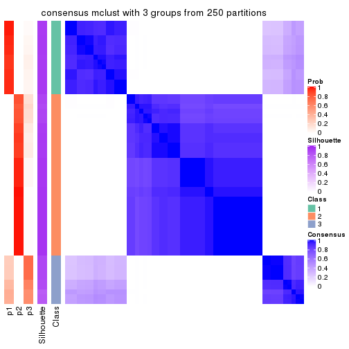
consensus_heatmap(res, k = 4)
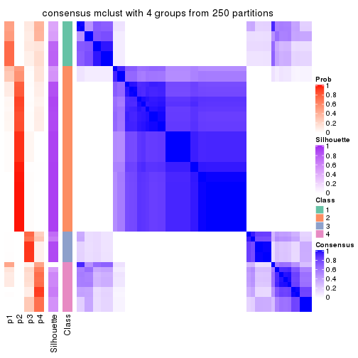
consensus_heatmap(res, k = 5)
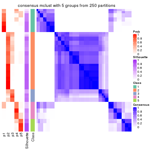
consensus_heatmap(res, k = 6)
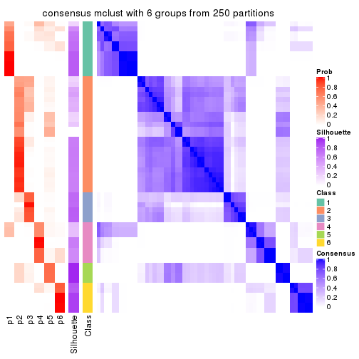
Heatmaps for the membership of samples in all partitions to see how consistent they are:
membership_heatmap(res, k = 2)

membership_heatmap(res, k = 3)
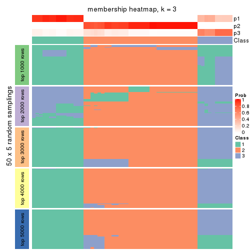
membership_heatmap(res, k = 4)
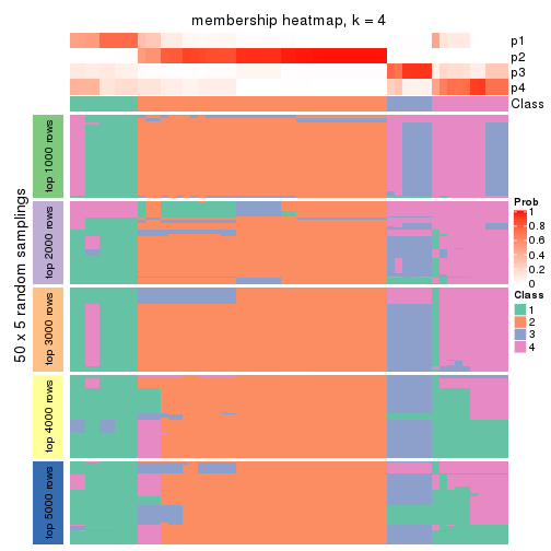
membership_heatmap(res, k = 5)
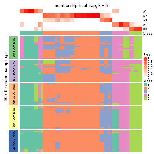
membership_heatmap(res, k = 6)
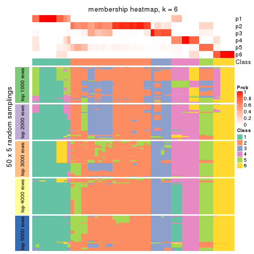
As soon as we have had the classes for columns, we can look for signatures which are significantly different between classes which can be candidate marks for certain classes. Following are the heatmaps for signatures.
Signature heatmaps where rows are scaled:
get_signatures(res, k = 2)

get_signatures(res, k = 3)
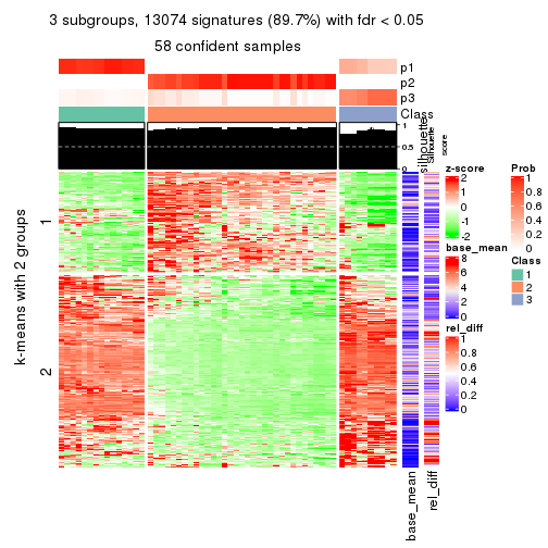
get_signatures(res, k = 4)
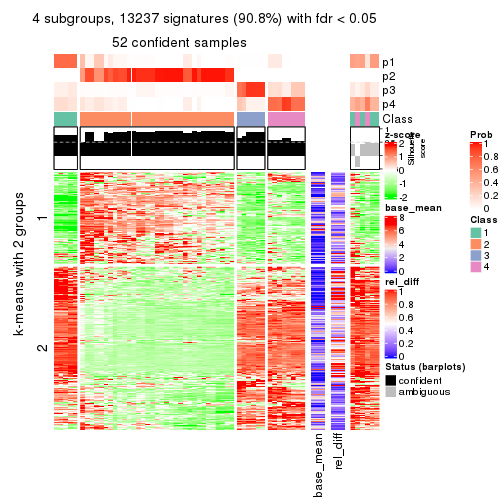
get_signatures(res, k = 5)
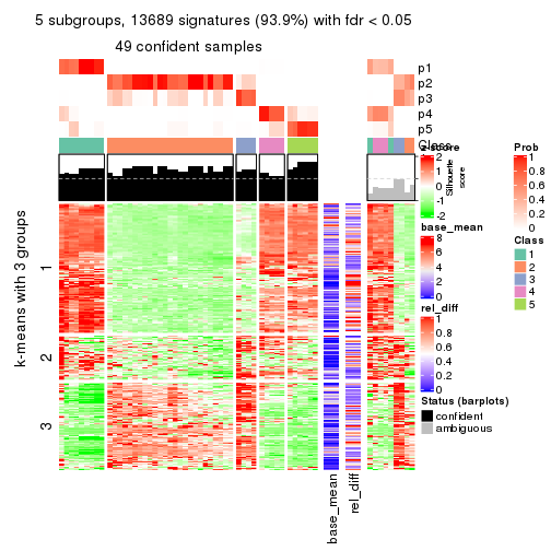
get_signatures(res, k = 6)
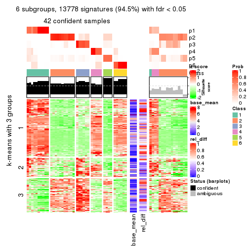
Signature heatmaps where rows are not scaled:
get_signatures(res, k = 2, scale_rows = FALSE)

get_signatures(res, k = 3, scale_rows = FALSE)
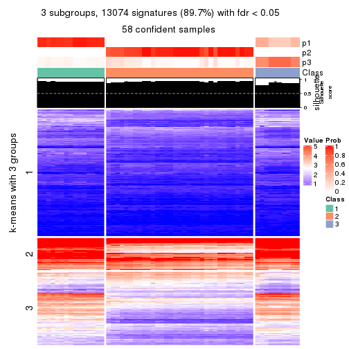
get_signatures(res, k = 4, scale_rows = FALSE)
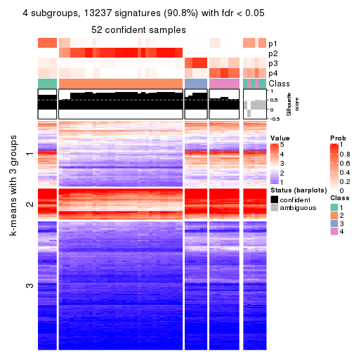
get_signatures(res, k = 5, scale_rows = FALSE)
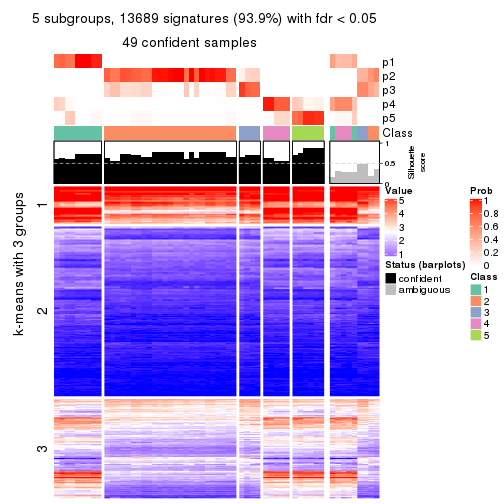
get_signatures(res, k = 6, scale_rows = FALSE)
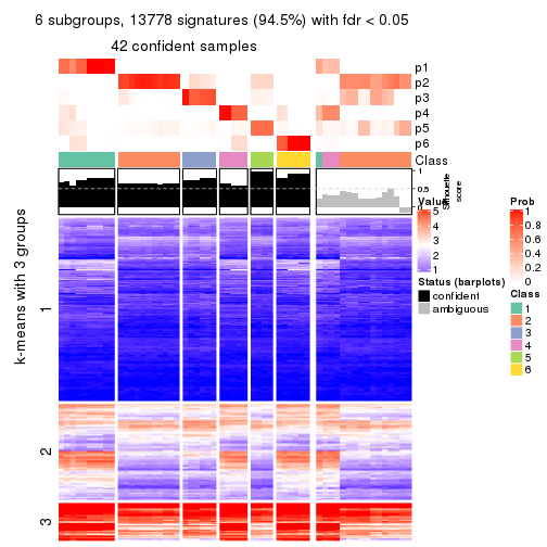
Compare the overlap of signatures from different k:
compare_signatures(res)
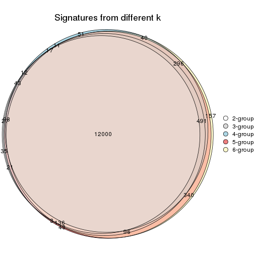
get_signature() returns a data frame invisibly. TO get the list of signatures, the function
call should be assigned to a variable explicitly. In following code, if plot argument is set
to FALSE, no heatmap is plotted while only the differential analysis is performed.
# code only for demonstration
tb = get_signature(res, k = ..., plot = FALSE)
An example of the output of tb is:
#>   which_row         fdr    mean_1    mean_2 scaled_mean_1 scaled_mean_2 km
#> 1        38 0.042760348  8.373488  9.131774    -0.5533452     0.5164555  1
#> 2        40 0.018707592  7.106213  8.469186    -0.6173731     0.5762149  1
#> 3        55 0.019134737 10.221463 11.207825    -0.6159697     0.5749050  1
#> 4        59 0.006059896  5.921854  7.869574    -0.6899429     0.6439467  1
#> 5        60 0.018055526  8.928898 10.211722    -0.6204761     0.5791110  1
#> 6        98 0.009384629 15.714769 14.887706     0.6635654    -0.6193277  2
...
The columns in tb are:
which_row: row indices corresponding to the input matrix.fdr: FDR for the differential test. mean_x: The mean value in group x.scaled_mean_x: The mean value in group x after rows are scaled.km: Row groups if k-means clustering is applied to rows.UMAP plot which shows how samples are separated.
dimension_reduction(res, k = 2, method = "UMAP")
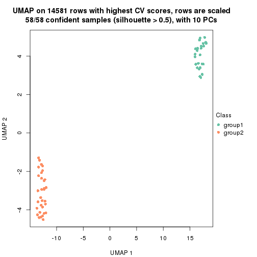
dimension_reduction(res, k = 3, method = "UMAP")

dimension_reduction(res, k = 4, method = "UMAP")
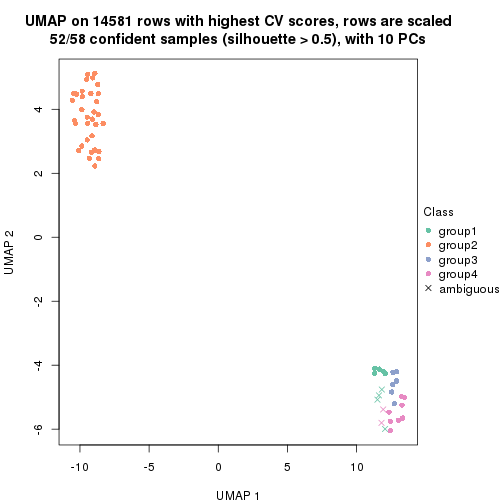
dimension_reduction(res, k = 5, method = "UMAP")
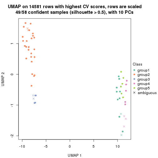
dimension_reduction(res, k = 6, method = "UMAP")
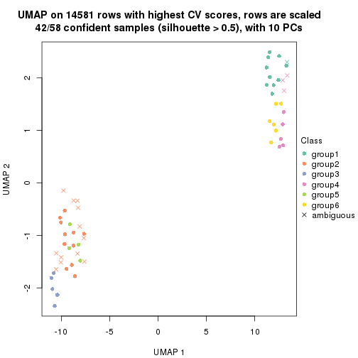
Following heatmap shows how subgroups are split when increasing k:
collect_classes(res)
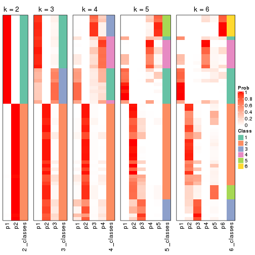
If matrix rows can be associated to genes, consider to use functional_enrichment(res,
...) to perform function enrichment for the signature genes. See this vignette for more detailed explanations.
The object with results only for a single top-value method and a single partition method can be extracted as:
res = res_list["CV", "NMF"]
# you can also extract it by
# res = res_list["CV:NMF"]
A summary of res and all the functions that can be applied to it:
res
#> A 'ConsensusPartition' object with k = 2, 3, 4, 5, 6.
#>   On a matrix with 14581 rows and 58 columns.
#>   Top rows (1000, 2000, 3000, 4000, 5000) are extracted by 'CV' method.
#>   Subgroups are detected by 'NMF' method.
#>   Performed in total 1250 partitions by row resampling.
#>   Best k for subgroups seems to be 3.
#>
#> Following methods can be applied to this 'ConsensusPartition' object:
#>  [1] "cola_report"             "collect_classes"         "collect_plots"
#>  [4] "collect_stats"           "colnames"                "compare_signatures"
#>  [7] "consensus_heatmap"       "dimension_reduction"     "functional_enrichment"
#> [10] "get_anno_col"            "get_anno"                "get_classes"
#> [13] "get_consensus"           "get_matrix"              "get_membership"
#> [16] "get_param"               "get_signatures"          "get_stats"
#> [19] "is_best_k"               "is_stable_k"             "membership_heatmap"
#> [22] "ncol"                    "nrow"                    "plot_ecdf"
#> [25] "rownames"                "select_partition_number" "show"
#> [28] "suggest_best_k"          "test_to_known_factors"
collect_plots() function collects all the plots made from res for all k (number of partitions)
into one single page to provide an easy and fast comparison between different k.
collect_plots(res)
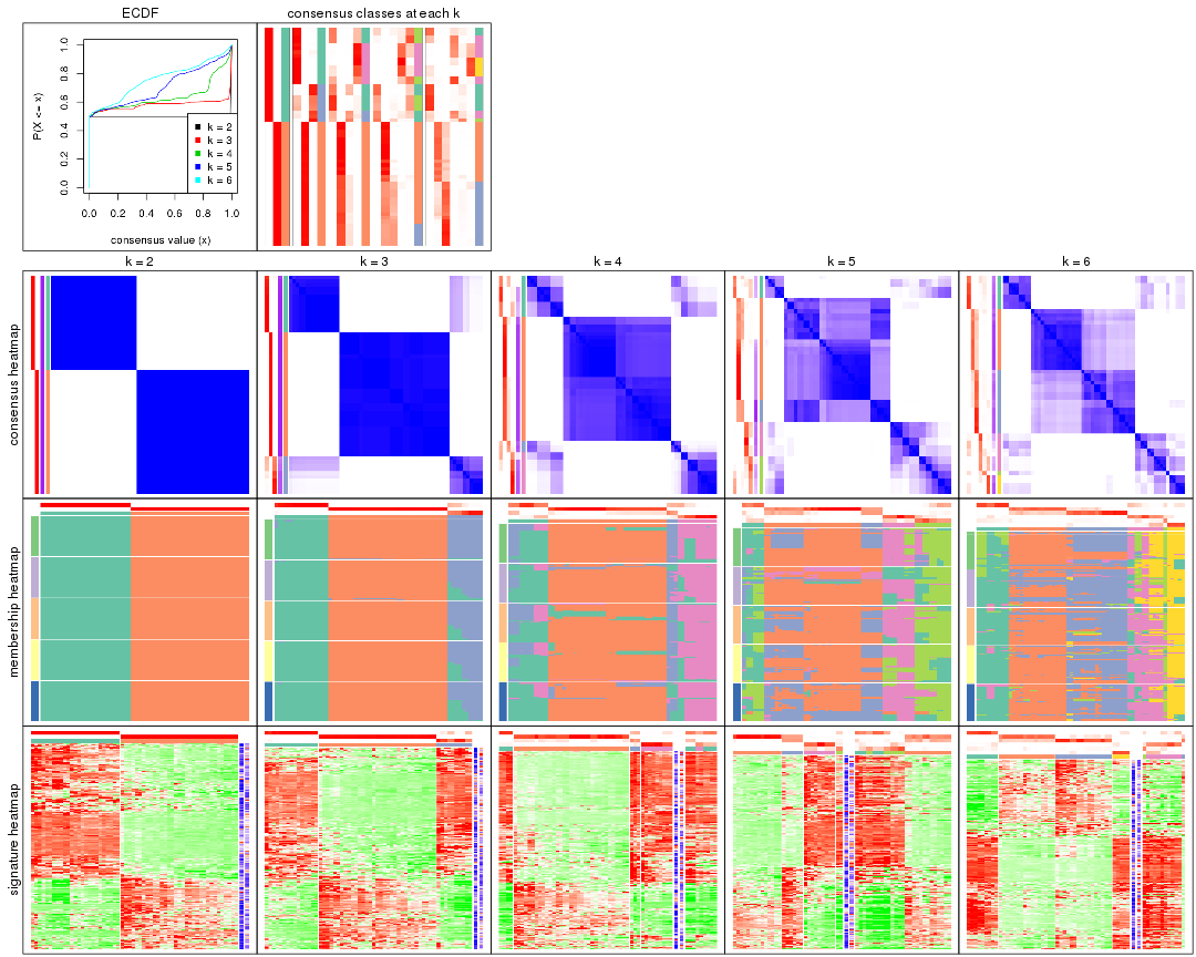
The plots are:
k and the heatmap of
predicted classes for each k.k.k.k.All the plots in panels can be made by individual functions and they are plotted later in this section.
select_partition_number() produces several plots showing different
statistics for choosing “optimized” k. There are following statistics:
k;k, the area increased is defined as \(A_k - A_{k-1}\).The detailed explanations of these statistics can be found in the cola vignette.
Generally speaking, lower PAC score, higher mean silhouette score or higher
concordance corresponds to better partition. Rand index and Jaccard index
measure how similar the current partition is compared to partition with k-1.
If they are too similar, we won't accept k is better than k-1.
select_partition_number(res)
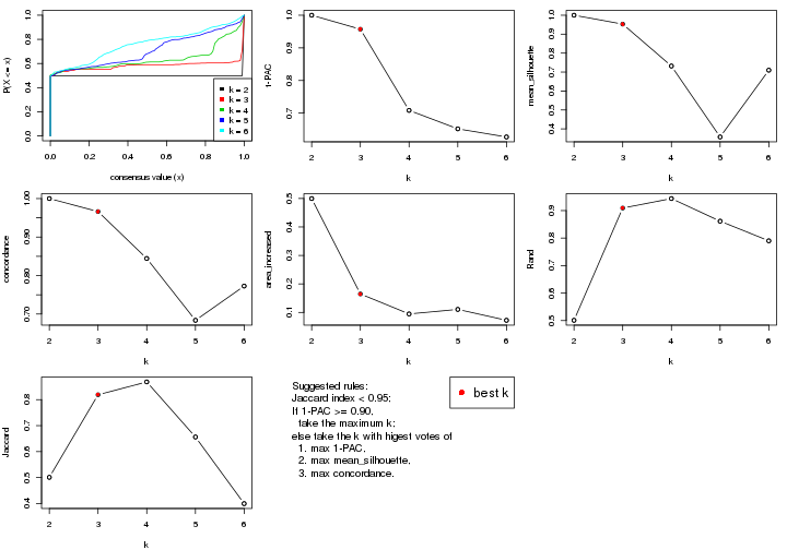
The numeric values for all these statistics can be obtained by get_stats().
get_stats(res)
#>   k 1-PAC mean_silhouette concordance area_increased  Rand Jaccard
#> 2 2 1.000           1.000       1.000         0.4996 0.501   0.501
#> 3 3 0.957           0.953       0.966         0.1648 0.909   0.819
#> 4 4 0.708           0.732       0.844         0.0947 0.944   0.868
#> 5 5 0.652           0.357       0.684         0.1106 0.861   0.656
#> 6 6 0.627           0.710       0.773         0.0724 0.790   0.400
suggest_best_k() suggests the best \(k\) based on these statistics. The rules are as follows:
suggest_best_k(res)
#> [1] 3
#> attr(,"optional")
#> [1] 2
There is also optional best \(k\) = 2 that is worth to check.
Following shows the table of the partitions (You need to click the show/hide
code output link to see it). The membership matrix (columns with name p*)
is inferred by
clue::cl_consensus()
function with the SE method. Basically the value in the membership matrix
represents the probability to belong to a certain group. The finall class
label for an item is determined with the group with highest probability it
belongs to.
In get_classes() function, the entropy is calculated from the membership
matrix and the silhouette score is calculated from the consensus matrix.
cbind(get_classes(res, k = 2), get_membership(res, k = 2))
#>           class entropy silhouette p1 p2
#> ERR789082     2       0          1  0  1
#> ERR789083     2       0          1  0  1
#> ERR789191     2       0          1  0  1
#> ERR789192     2       0          1  0  1
#> ERR789213     1       0          1  1  0
#> ERR789385     1       0          1  1  0
#> ERR789393     1       0          1  1  0
#> ERR789394     1       0          1  1  0
#> ERR789193     2       0          1  0  1
#> ERR789194     2       0          1  0  1
#> ERR789195     2       0          1  0  1
#> ERR789196     2       0          1  0  1
#> ERR789388     1       0          1  1  0
#> ERR789197     2       0          1  0  1
#> ERR789198     2       0          1  0  1
#> ERR789214     1       0          1  1  0
#> ERR789397     1       0          1  1  0
#> ERR789398     1       0          1  1  0
#> ERR789199     2       0          1  0  1
#> ERR789200     2       0          1  0  1
#> ERR789201     2       0          1  0  1
#> ERR789202     2       0          1  0  1
#> ERR789215     1       0          1  1  0
#> ERR789203     2       0          1  0  1
#> ERR789204     2       0          1  0  1
#> ERR789383     1       0          1  1  0
#> ERR789205     2       0          1  0  1
#> ERR789206     2       0          1  0  1
#> ERR789399     1       0          1  1  0
#> ERR789400     1       0          1  1  0
#> ERR789207     2       0          1  0  1
#> ERR789208     2       0          1  0  1
#> ERR789209     2       0          1  0  1
#> ERR789210     2       0          1  0  1
#> ERR789211     2       0          1  0  1
#> ERR789212     2       0          1  0  1
#> ERR789386     1       0          1  1  0
#> ERR789076     2       0          1  0  1
#> ERR789077     2       0          1  0  1
#> ERR789384     1       0          1  1  0
#> ERR789078     2       0          1  0  1
#> ERR789079     2       0          1  0  1
#> ERR789216     1       0          1  1  0
#> ERR789080     2       0          1  0  1
#> ERR789387     1       0          1  1  0
#> ERR789081     2       0          1  0  1
#> ERR789064     2       0          1  0  1
#> ERR779485     2       0          1  0  1
#> ERR789065     2       0          1  0  1
#> ERR789401     1       0          1  1  0
#> ERR789402     1       0          1  1  0
#> ERR789403     1       0          1  1  0
#> ERR789389     1       0          1  1  0
#> ERR789395     1       0          1  1  0
#> ERR789396     1       0          1  1  0
#> ERR789390     1       0          1  1  0
#> ERR789391     1       0          1  1  0
#> ERR789392     1       0          1  1  0
cbind(get_classes(res, k = 3), get_membership(res, k = 3))
#>           class entropy silhouette    p1    p2    p3
#> ERR789082     2  0.0237      0.995 0.000 0.996 0.004
#> ERR789083     2  0.0237      0.995 0.000 0.996 0.004
#> ERR789191     2  0.0000      0.996 0.000 1.000 0.000
#> ERR789192     2  0.0000      0.996 0.000 1.000 0.000
#> ERR789213     1  0.0000      0.990 1.000 0.000 0.000
#> ERR789385     1  0.0000      0.990 1.000 0.000 0.000
#> ERR789393     1  0.0000      0.990 1.000 0.000 0.000
#> ERR789394     1  0.0000      0.990 1.000 0.000 0.000
#> ERR789193     2  0.0237      0.995 0.000 0.996 0.004
#> ERR789194     2  0.0237      0.995 0.000 0.996 0.004
#> ERR789195     2  0.0237      0.996 0.000 0.996 0.004
#> ERR789196     2  0.0237      0.996 0.000 0.996 0.004
#> ERR789388     1  0.0000      0.990 1.000 0.000 0.000
#> ERR789197     2  0.0237      0.996 0.000 0.996 0.004
#> ERR789198     2  0.0237      0.996 0.000 0.996 0.004
#> ERR789214     1  0.0000      0.990 1.000 0.000 0.000
#> ERR789397     1  0.0000      0.990 1.000 0.000 0.000
#> ERR789398     1  0.0000      0.990 1.000 0.000 0.000
#> ERR789199     2  0.0237      0.996 0.000 0.996 0.004
#> ERR789200     2  0.0237      0.996 0.000 0.996 0.004
#> ERR789201     2  0.0424      0.995 0.000 0.992 0.008
#> ERR789202     2  0.0424      0.995 0.000 0.992 0.008
#> ERR789215     3  0.2878      0.827 0.096 0.000 0.904
#> ERR789203     2  0.0424      0.995 0.000 0.992 0.008
#> ERR789204     2  0.0424      0.995 0.000 0.992 0.008
#> ERR789383     3  0.3412      0.822 0.124 0.000 0.876
#> ERR789205     2  0.0424      0.995 0.000 0.992 0.008
#> ERR789206     2  0.0424      0.995 0.000 0.992 0.008
#> ERR789399     3  0.5706      0.720 0.320 0.000 0.680
#> ERR789400     3  0.5706      0.720 0.320 0.000 0.680
#> ERR789207     2  0.0237      0.995 0.000 0.996 0.004
#> ERR789208     2  0.0237      0.995 0.000 0.996 0.004
#> ERR789209     2  0.0000      0.996 0.000 1.000 0.000
#> ERR789210     2  0.0000      0.996 0.000 1.000 0.000
#> ERR789211     2  0.0237      0.995 0.000 0.996 0.004
#> ERR789212     2  0.0237      0.995 0.000 0.996 0.004
#> ERR789386     1  0.0747      0.979 0.984 0.000 0.016
#> ERR789076     2  0.0424      0.995 0.000 0.992 0.008
#> ERR789077     2  0.0237      0.995 0.000 0.996 0.004
#> ERR789384     1  0.0000      0.990 1.000 0.000 0.000
#> ERR789078     2  0.0424      0.995 0.000 0.992 0.008
#> ERR789079     2  0.0237      0.995 0.000 0.996 0.004
#> ERR789216     1  0.1964      0.929 0.944 0.000 0.056
#> ERR789080     2  0.0424      0.995 0.000 0.992 0.008
#> ERR789387     3  0.0747      0.817 0.016 0.000 0.984
#> ERR789081     2  0.0424      0.995 0.000 0.992 0.008
#> ERR789064     2  0.0424      0.995 0.000 0.992 0.008
#> ERR779485     2  0.0592      0.994 0.000 0.988 0.012
#> ERR789065     2  0.0424      0.995 0.000 0.992 0.008
#> ERR789401     3  0.5882      0.685 0.348 0.000 0.652
#> ERR789402     3  0.1031      0.823 0.024 0.000 0.976
#> ERR789403     3  0.6062      0.623 0.384 0.000 0.616
#> ERR789389     1  0.0892      0.974 0.980 0.000 0.020
#> ERR789395     3  0.1031      0.823 0.024 0.000 0.976
#> ERR789396     3  0.1031      0.823 0.024 0.000 0.976
#> ERR789390     1  0.0424      0.986 0.992 0.000 0.008
#> ERR789391     1  0.0424      0.986 0.992 0.000 0.008
#> ERR789392     1  0.0000      0.990 1.000 0.000 0.000
cbind(get_classes(res, k = 4), get_membership(res, k = 4))
#>           class entropy silhouette    p1    p2    p3    p4
#> ERR789082     2  0.0188      0.919 0.000 0.996 0.004 0.000
#> ERR789083     2  0.0000      0.919 0.000 1.000 0.000 0.000
#> ERR789191     2  0.1118      0.922 0.000 0.964 0.036 0.000
#> ERR789192     2  0.1022      0.922 0.000 0.968 0.032 0.000
#> ERR789213     4  0.0000      0.819 0.000 0.000 0.000 1.000
#> ERR789385     4  0.0000      0.819 0.000 0.000 0.000 1.000
#> ERR789393     4  0.3172      0.743 0.160 0.000 0.000 0.840
#> ERR789394     4  0.2973      0.755 0.144 0.000 0.000 0.856
#> ERR789193     2  0.2921      0.921 0.000 0.860 0.140 0.000
#> ERR789194     2  0.2868      0.922 0.000 0.864 0.136 0.000
#> ERR789195     2  0.3172      0.915 0.000 0.840 0.160 0.000
#> ERR789196     2  0.3172      0.915 0.000 0.840 0.160 0.000
#> ERR789388     4  0.5088      0.117 0.424 0.000 0.004 0.572
#> ERR789197     2  0.3074      0.918 0.000 0.848 0.152 0.000
#> ERR789198     2  0.3074      0.918 0.000 0.848 0.152 0.000
#> ERR789214     4  0.5070      0.142 0.416 0.000 0.004 0.580
#> ERR789397     1  0.4837      0.362 0.648 0.000 0.004 0.348
#> ERR789398     1  0.4837      0.362 0.648 0.000 0.004 0.348
#> ERR789199     2  0.3074      0.918 0.000 0.848 0.152 0.000
#> ERR789200     2  0.3074      0.918 0.000 0.848 0.152 0.000
#> ERR789201     2  0.2281      0.925 0.000 0.904 0.096 0.000
#> ERR789202     2  0.2469      0.924 0.000 0.892 0.108 0.000
#> ERR789215     3  0.6376      0.855 0.396 0.000 0.536 0.068
#> ERR789203     2  0.3074      0.918 0.000 0.848 0.152 0.000
#> ERR789204     2  0.3074      0.918 0.000 0.848 0.152 0.000
#> ERR789383     3  0.7049      0.822 0.392 0.000 0.484 0.124
#> ERR789205     2  0.3219      0.914 0.000 0.836 0.164 0.000
#> ERR789206     2  0.3219      0.914 0.000 0.836 0.164 0.000
#> ERR789399     1  0.1557      0.532 0.944 0.000 0.000 0.056
#> ERR789400     1  0.1743      0.530 0.940 0.000 0.004 0.056
#> ERR789207     2  0.0000      0.919 0.000 1.000 0.000 0.000
#> ERR789208     2  0.0000      0.919 0.000 1.000 0.000 0.000
#> ERR789209     2  0.0000      0.919 0.000 1.000 0.000 0.000
#> ERR789210     2  0.0000      0.919 0.000 1.000 0.000 0.000
#> ERR789211     2  0.0000      0.919 0.000 1.000 0.000 0.000
#> ERR789212     2  0.0000      0.919 0.000 1.000 0.000 0.000
#> ERR789386     4  0.0524      0.820 0.008 0.000 0.004 0.988
#> ERR789076     2  0.0469      0.918 0.000 0.988 0.012 0.000
#> ERR789077     2  0.0000      0.919 0.000 1.000 0.000 0.000
#> ERR789384     4  0.0524      0.820 0.008 0.000 0.004 0.988
#> ERR789078     2  0.0817      0.910 0.000 0.976 0.024 0.000
#> ERR789079     2  0.0188      0.917 0.000 0.996 0.004 0.000
#> ERR789216     4  0.0657      0.812 0.012 0.000 0.004 0.984
#> ERR789080     2  0.3074      0.803 0.000 0.848 0.152 0.000
#> ERR789387     3  0.5460      0.798 0.340 0.000 0.632 0.028
#> ERR789081     2  0.2973      0.812 0.000 0.856 0.144 0.000
#> ERR789064     2  0.2345      0.925 0.000 0.900 0.100 0.000
#> ERR779485     2  0.3219      0.915 0.000 0.836 0.164 0.000
#> ERR789065     2  0.3172      0.916 0.000 0.840 0.160 0.000
#> ERR789401     1  0.1970      0.528 0.932 0.000 0.008 0.060
#> ERR789402     1  0.4605     -0.358 0.664 0.000 0.336 0.000
#> ERR789403     1  0.1716      0.535 0.936 0.000 0.000 0.064
#> ERR789389     4  0.0336      0.820 0.008 0.000 0.000 0.992
#> ERR789395     1  0.4643     -0.378 0.656 0.000 0.344 0.000
#> ERR789396     1  0.4746     -0.440 0.632 0.000 0.368 0.000
#> ERR789390     1  0.4585      0.400 0.668 0.000 0.000 0.332
#> ERR789391     1  0.4624      0.387 0.660 0.000 0.000 0.340
#> ERR789392     4  0.2973      0.755 0.144 0.000 0.000 0.856
cbind(get_classes(res, k = 5), get_membership(res, k = 5))
#>           class entropy silhouette    p1    p2    p3    p4    p5
#> ERR789082     2  0.0404      0.595 0.000 0.988 0.012 0.000 0.000
#> ERR789083     2  0.0162      0.597 0.000 0.996 0.004 0.000 0.000
#> ERR789191     2  0.0566      0.593 0.000 0.984 0.012 0.000 0.004
#> ERR789192     2  0.0451      0.595 0.000 0.988 0.008 0.000 0.004
#> ERR789213     4  0.0000      0.753 0.000 0.000 0.000 1.000 0.000
#> ERR789385     4  0.0000      0.753 0.000 0.000 0.000 1.000 0.000
#> ERR789393     4  0.3053      0.683 0.000 0.000 0.008 0.828 0.164
#> ERR789394     4  0.2971      0.692 0.000 0.000 0.008 0.836 0.156
#> ERR789193     2  0.5420     -0.513 0.000 0.548 0.396 0.052 0.004
#> ERR789194     2  0.5420     -0.513 0.000 0.548 0.396 0.052 0.004
#> ERR789195     2  0.4627     -0.771 0.000 0.544 0.444 0.000 0.012
#> ERR789196     2  0.4627     -0.771 0.000 0.544 0.444 0.000 0.012
#> ERR789388     5  0.3969      0.176 0.000 0.000 0.004 0.304 0.692
#> ERR789197     2  0.4557     -0.634 0.000 0.584 0.404 0.000 0.012
#> ERR789198     2  0.4557     -0.634 0.000 0.584 0.404 0.000 0.012
#> ERR789214     5  0.4218      0.112 0.004 0.000 0.004 0.324 0.668
#> ERR789397     5  0.3291      0.463 0.040 0.000 0.000 0.120 0.840
#> ERR789398     5  0.3291      0.463 0.040 0.000 0.000 0.120 0.840
#> ERR789199     2  0.4470     -0.520 0.000 0.616 0.372 0.000 0.012
#> ERR789200     2  0.4444     -0.489 0.000 0.624 0.364 0.000 0.012
#> ERR789201     2  0.4147     -0.242 0.000 0.676 0.316 0.000 0.008
#> ERR789202     2  0.4489     -0.682 0.000 0.572 0.420 0.000 0.008
#> ERR789215     1  0.5931      0.440 0.616 0.000 0.020 0.096 0.268
#> ERR789203     3  0.4559      0.974 0.000 0.480 0.512 0.000 0.008
#> ERR789204     3  0.4559      0.974 0.000 0.480 0.512 0.000 0.008
#> ERR789383     1  0.6438      0.436 0.596 0.000 0.036 0.132 0.236
#> ERR789205     3  0.4448      0.976 0.000 0.480 0.516 0.000 0.004
#> ERR789206     3  0.4446      0.975 0.000 0.476 0.520 0.000 0.004
#> ERR789399     5  0.4973      0.289 0.480 0.000 0.020 0.004 0.496
#> ERR789400     5  0.5190      0.307 0.468 0.000 0.032 0.004 0.496
#> ERR789207     2  0.0290      0.595 0.000 0.992 0.008 0.000 0.000
#> ERR789208     2  0.0290      0.595 0.000 0.992 0.008 0.000 0.000
#> ERR789209     2  0.0000      0.598 0.000 1.000 0.000 0.000 0.000
#> ERR789210     2  0.0000      0.598 0.000 1.000 0.000 0.000 0.000
#> ERR789211     2  0.0000      0.598 0.000 1.000 0.000 0.000 0.000
#> ERR789212     2  0.0000      0.598 0.000 1.000 0.000 0.000 0.000
#> ERR789386     4  0.4003      0.688 0.008 0.000 0.000 0.704 0.288
#> ERR789076     2  0.2136      0.524 0.000 0.904 0.088 0.000 0.008
#> ERR789077     2  0.0162      0.597 0.000 0.996 0.004 0.000 0.000
#> ERR789384     4  0.3662      0.723 0.004 0.000 0.000 0.744 0.252
#> ERR789078     2  0.1408      0.570 0.000 0.948 0.044 0.000 0.008
#> ERR789079     2  0.0324      0.596 0.000 0.992 0.004 0.000 0.004
#> ERR789216     4  0.3863      0.724 0.012 0.000 0.000 0.740 0.248
#> ERR789080     2  0.4159      0.408 0.000 0.776 0.156 0.000 0.068
#> ERR789387     1  0.5007      0.422 0.688 0.000 0.256 0.032 0.024
#> ERR789081     2  0.3182      0.469 0.000 0.844 0.124 0.000 0.032
#> ERR789064     2  0.4559     -0.918 0.000 0.512 0.480 0.000 0.008
#> ERR779485     3  0.4450      0.966 0.000 0.488 0.508 0.004 0.000
#> ERR789065     3  0.4450      0.969 0.000 0.488 0.508 0.000 0.004
#> ERR789401     5  0.5735      0.354 0.428 0.000 0.056 0.012 0.504
#> ERR789402     1  0.3689      0.394 0.740 0.000 0.004 0.000 0.256
#> ERR789403     5  0.5735      0.354 0.428 0.000 0.056 0.012 0.504
#> ERR789389     4  0.3689      0.721 0.004 0.000 0.000 0.740 0.256
#> ERR789395     1  0.3508      0.396 0.748 0.000 0.000 0.000 0.252
#> ERR789396     1  0.3550      0.417 0.760 0.000 0.004 0.000 0.236
#> ERR789390     5  0.6385      0.502 0.236 0.000 0.056 0.096 0.612
#> ERR789391     5  0.6427      0.503 0.228 0.000 0.056 0.104 0.612
#> ERR789392     4  0.2971      0.692 0.000 0.000 0.008 0.836 0.156
cbind(get_classes(res, k = 6), get_membership(res, k = 6))
#>           class entropy silhouette    p1    p2    p3    p4    p5    p6
#> ERR789082     2  0.3244    0.90854 0.000 0.732 0.268 0.000 0.000 0.000
#> ERR789083     2  0.3175    0.91569 0.000 0.744 0.256 0.000 0.000 0.000
#> ERR789191     2  0.3541    0.90828 0.000 0.728 0.260 0.000 0.012 0.000
#> ERR789192     2  0.3445    0.91087 0.000 0.732 0.260 0.000 0.008 0.000
#> ERR789213     6  0.2048    0.75911 0.000 0.000 0.000 0.120 0.000 0.880
#> ERR789385     6  0.2442    0.73506 0.000 0.000 0.000 0.144 0.004 0.852
#> ERR789393     6  0.2558    0.83152 0.156 0.000 0.000 0.004 0.000 0.840
#> ERR789394     6  0.2320    0.84092 0.132 0.000 0.000 0.004 0.000 0.864
#> ERR789193     3  0.4321    0.69322 0.000 0.140 0.744 0.000 0.008 0.108
#> ERR789194     3  0.4486    0.67870 0.000 0.140 0.728 0.000 0.008 0.124
#> ERR789195     3  0.3569    0.79770 0.000 0.124 0.816 0.008 0.044 0.008
#> ERR789196     3  0.3569    0.79770 0.000 0.124 0.816 0.008 0.044 0.008
#> ERR789388     4  0.2655    0.45514 0.060 0.020 0.000 0.884 0.000 0.036
#> ERR789197     3  0.3886    0.76133 0.000 0.164 0.780 0.008 0.040 0.008
#> ERR789198     3  0.3851    0.76506 0.000 0.160 0.784 0.008 0.040 0.008
#> ERR789214     4  0.2981    0.44879 0.048 0.036 0.000 0.868 0.000 0.048
#> ERR789397     4  0.4303    0.23596 0.332 0.012 0.000 0.640 0.000 0.016
#> ERR789398     4  0.4337    0.26023 0.320 0.012 0.000 0.648 0.000 0.020
#> ERR789199     3  0.4260    0.70159 0.000 0.212 0.732 0.008 0.040 0.008
#> ERR789200     3  0.4340    0.68124 0.000 0.224 0.720 0.008 0.040 0.008
#> ERR789201     3  0.4370    0.47359 0.000 0.284 0.676 0.004 0.028 0.008
#> ERR789202     3  0.3416    0.76219 0.000 0.140 0.816 0.004 0.032 0.008
#> ERR789215     4  0.5716    0.08277 0.192 0.016 0.000 0.628 0.148 0.016
#> ERR789203     3  0.1036    0.80874 0.000 0.008 0.964 0.000 0.024 0.004
#> ERR789204     3  0.1036    0.80874 0.000 0.008 0.964 0.000 0.024 0.004
#> ERR789383     4  0.6441   -0.00432 0.236 0.012 0.000 0.548 0.160 0.044
#> ERR789205     3  0.0622    0.81816 0.000 0.012 0.980 0.000 0.008 0.000
#> ERR789206     3  0.0964    0.81903 0.000 0.016 0.968 0.004 0.012 0.000
#> ERR789399     1  0.2001    0.81028 0.924 0.012 0.000 0.028 0.032 0.004
#> ERR789400     1  0.1844    0.81217 0.932 0.012 0.000 0.028 0.024 0.004
#> ERR789207     2  0.2933    0.91260 0.000 0.796 0.200 0.000 0.000 0.004
#> ERR789208     2  0.2823    0.91770 0.000 0.796 0.204 0.000 0.000 0.000
#> ERR789209     2  0.3136    0.92820 0.000 0.768 0.228 0.000 0.000 0.004
#> ERR789210     2  0.2969    0.92793 0.000 0.776 0.224 0.000 0.000 0.000
#> ERR789211     2  0.2996    0.92792 0.000 0.772 0.228 0.000 0.000 0.000
#> ERR789212     2  0.2941    0.92653 0.000 0.780 0.220 0.000 0.000 0.000
#> ERR789386     4  0.4990    0.46628 0.012 0.000 0.000 0.600 0.060 0.328
#> ERR789076     2  0.3955    0.77064 0.000 0.608 0.384 0.000 0.008 0.000
#> ERR789077     2  0.3050    0.92783 0.000 0.764 0.236 0.000 0.000 0.000
#> ERR789384     4  0.5000    0.44923 0.012 0.000 0.000 0.584 0.056 0.348
#> ERR789078     2  0.3758    0.84746 0.000 0.668 0.324 0.000 0.008 0.000
#> ERR789079     2  0.2969    0.92674 0.000 0.776 0.224 0.000 0.000 0.000
#> ERR789216     4  0.5081    0.40819 0.008 0.000 0.000 0.552 0.064 0.376
#> ERR789080     2  0.4771    0.74440 0.000 0.652 0.248 0.000 0.100 0.000
#> ERR789387     5  0.5476    0.00000 0.188 0.000 0.000 0.164 0.628 0.020
#> ERR789081     2  0.3566    0.87896 0.000 0.744 0.236 0.000 0.020 0.000
#> ERR789064     3  0.1478    0.81506 0.000 0.032 0.944 0.000 0.020 0.004
#> ERR779485     3  0.1237    0.81742 0.000 0.020 0.956 0.000 0.004 0.020
#> ERR789065     3  0.1167    0.81614 0.000 0.012 0.960 0.000 0.008 0.020
#> ERR789401     1  0.1759    0.80837 0.924 0.004 0.000 0.004 0.064 0.004
#> ERR789402     1  0.2454    0.75228 0.876 0.000 0.000 0.016 0.104 0.004
#> ERR789403     1  0.1493    0.81124 0.936 0.000 0.000 0.004 0.056 0.004
#> ERR789389     4  0.5200    0.41060 0.012 0.000 0.000 0.552 0.068 0.368
#> ERR789395     1  0.2492    0.75206 0.876 0.000 0.000 0.020 0.100 0.004
#> ERR789396     1  0.2633    0.74005 0.864 0.000 0.000 0.020 0.112 0.004
#> ERR789390     1  0.4642    0.68583 0.732 0.008 0.000 0.164 0.080 0.016
#> ERR789391     1  0.4642    0.68583 0.732 0.008 0.000 0.164 0.080 0.016
#> ERR789392     6  0.2482    0.83901 0.148 0.000 0.000 0.004 0.000 0.848
Heatmaps for the consensus matrix. It visualizes the probability of two samples to be in a same group.
consensus_heatmap(res, k = 2)

consensus_heatmap(res, k = 3)
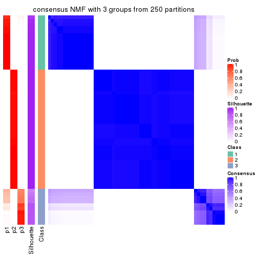
consensus_heatmap(res, k = 4)
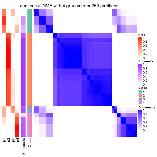
consensus_heatmap(res, k = 5)
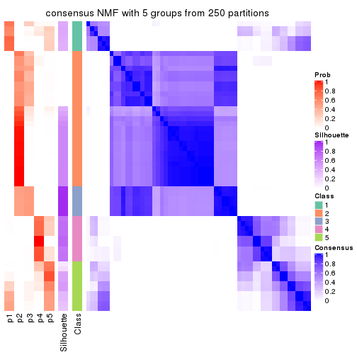
consensus_heatmap(res, k = 6)
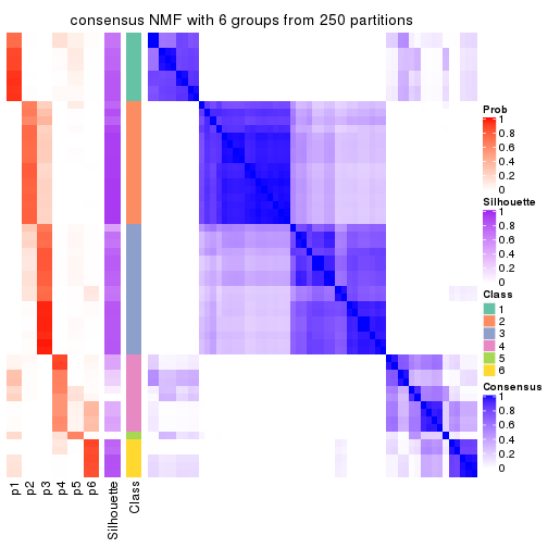
Heatmaps for the membership of samples in all partitions to see how consistent they are:
membership_heatmap(res, k = 2)

membership_heatmap(res, k = 3)
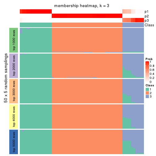
membership_heatmap(res, k = 4)
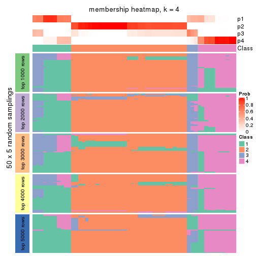
membership_heatmap(res, k = 5)
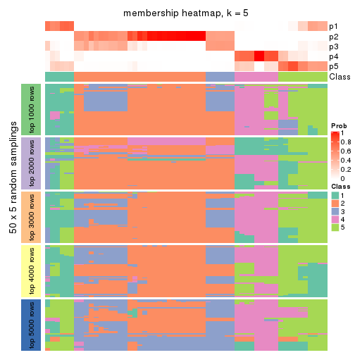
membership_heatmap(res, k = 6)
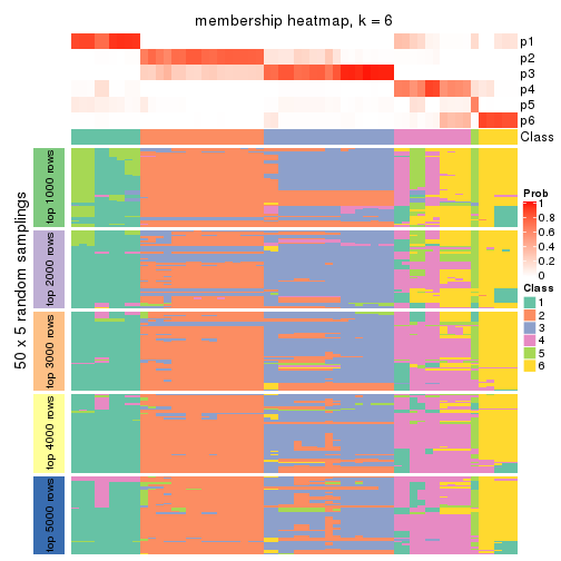
As soon as we have had the classes for columns, we can look for signatures which are significantly different between classes which can be candidate marks for certain classes. Following are the heatmaps for signatures.
Signature heatmaps where rows are scaled:
get_signatures(res, k = 2)

get_signatures(res, k = 3)
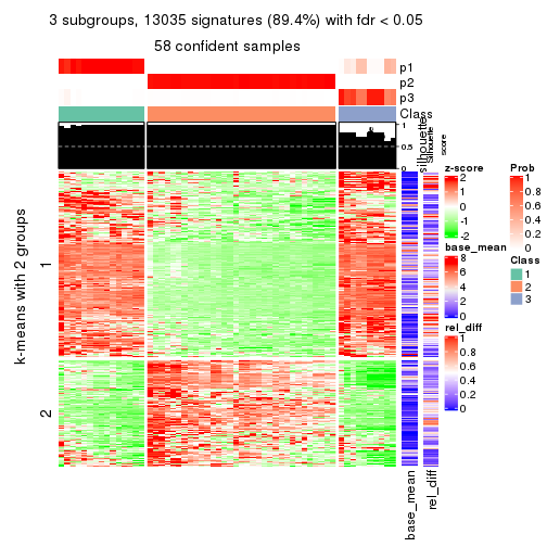
get_signatures(res, k = 4)
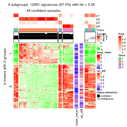
get_signatures(res, k = 5)
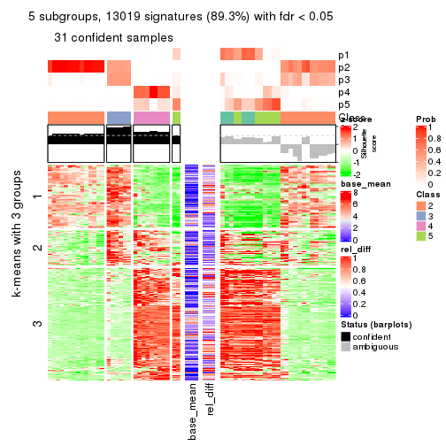
get_signatures(res, k = 6)
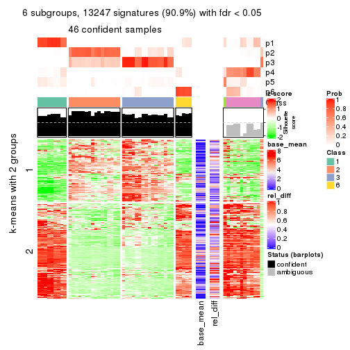
Signature heatmaps where rows are not scaled:
get_signatures(res, k = 2, scale_rows = FALSE)

get_signatures(res, k = 3, scale_rows = FALSE)
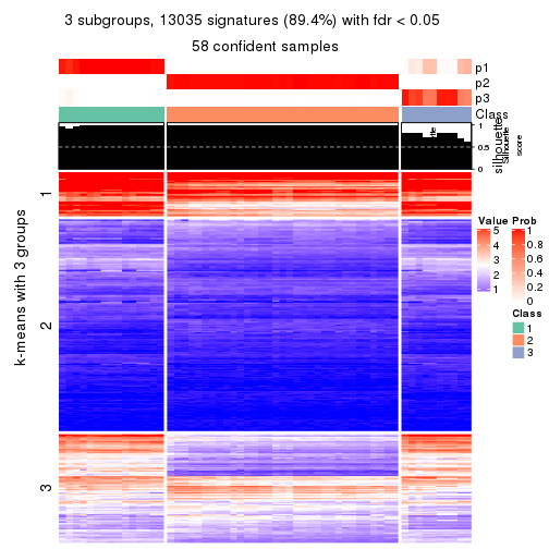
get_signatures(res, k = 4, scale_rows = FALSE)
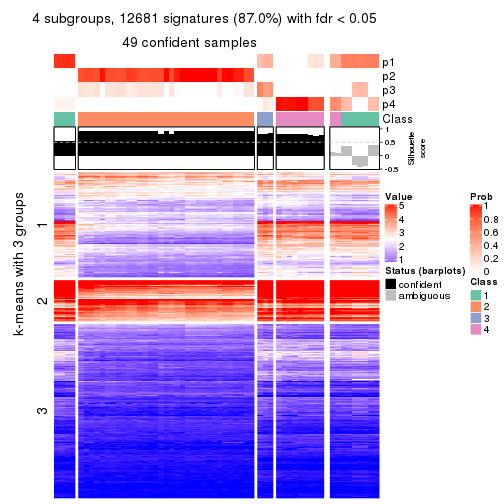
get_signatures(res, k = 5, scale_rows = FALSE)
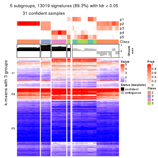
get_signatures(res, k = 6, scale_rows = FALSE)
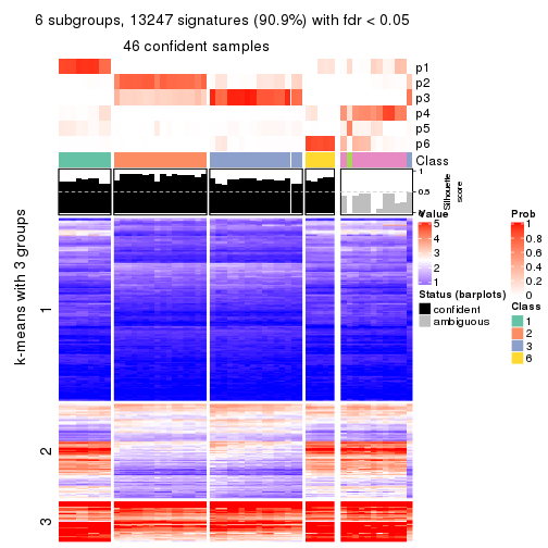
Compare the overlap of signatures from different k:
compare_signatures(res)
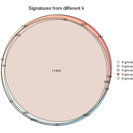
get_signature() returns a data frame invisibly. TO get the list of signatures, the function
call should be assigned to a variable explicitly. In following code, if plot argument is set
to FALSE, no heatmap is plotted while only the differential analysis is performed.
# code only for demonstration
tb = get_signature(res, k = ..., plot = FALSE)
An example of the output of tb is:
#>   which_row         fdr    mean_1    mean_2 scaled_mean_1 scaled_mean_2 km
#> 1        38 0.042760348  8.373488  9.131774    -0.5533452     0.5164555  1
#> 2        40 0.018707592  7.106213  8.469186    -0.6173731     0.5762149  1
#> 3        55 0.019134737 10.221463 11.207825    -0.6159697     0.5749050  1
#> 4        59 0.006059896  5.921854  7.869574    -0.6899429     0.6439467  1
#> 5        60 0.018055526  8.928898 10.211722    -0.6204761     0.5791110  1
#> 6        98 0.009384629 15.714769 14.887706     0.6635654    -0.6193277  2
...
The columns in tb are:
which_row: row indices corresponding to the input matrix.fdr: FDR for the differential test. mean_x: The mean value in group x.scaled_mean_x: The mean value in group x after rows are scaled.km: Row groups if k-means clustering is applied to rows.UMAP plot which shows how samples are separated.
dimension_reduction(res, k = 2, method = "UMAP")

dimension_reduction(res, k = 3, method = "UMAP")
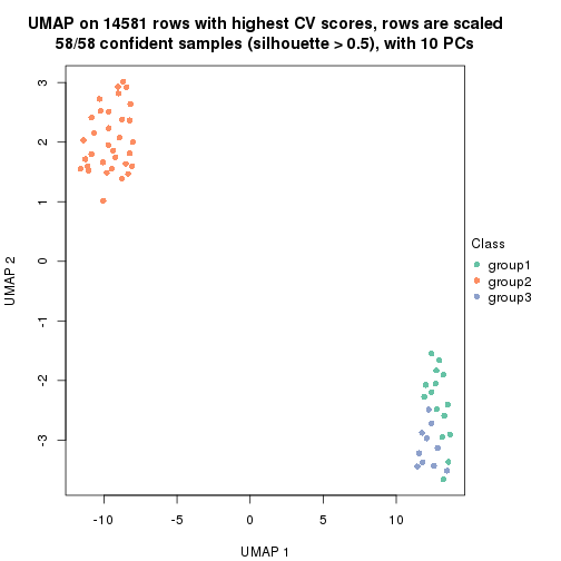
dimension_reduction(res, k = 4, method = "UMAP")
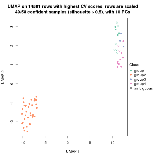
dimension_reduction(res, k = 5, method = "UMAP")
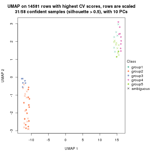
dimension_reduction(res, k = 6, method = "UMAP")
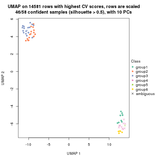
Following heatmap shows how subgroups are split when increasing k:
collect_classes(res)
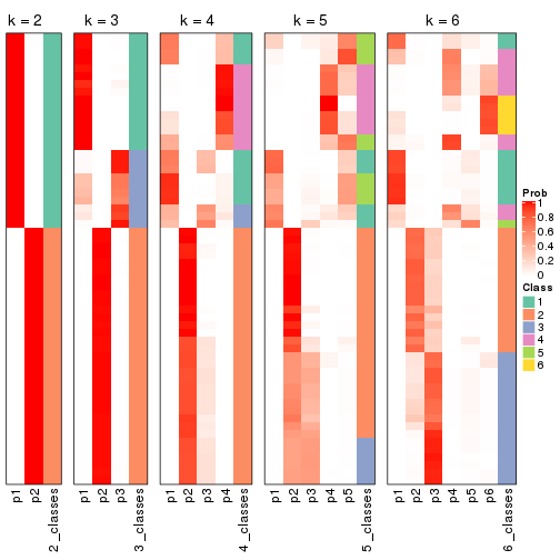
If matrix rows can be associated to genes, consider to use functional_enrichment(res,
...) to perform function enrichment for the signature genes. See this vignette for more detailed explanations.
The object with results only for a single top-value method and a single partition method can be extracted as:
res = res_list["MAD", "hclust"]
# you can also extract it by
# res = res_list["MAD:hclust"]
A summary of res and all the functions that can be applied to it:
res
#> A 'ConsensusPartition' object with k = 2, 3, 4, 5, 6.
#>   On a matrix with 14581 rows and 58 columns.
#>   Top rows (1000, 2000, 3000, 4000, 5000) are extracted by 'MAD' method.
#>   Subgroups are detected by 'hclust' method.
#>   Performed in total 1250 partitions by row resampling.
#>   Best k for subgroups seems to be 3.
#>
#> Following methods can be applied to this 'ConsensusPartition' object:
#>  [1] "cola_report"             "collect_classes"         "collect_plots"
#>  [4] "collect_stats"           "colnames"                "compare_signatures"
#>  [7] "consensus_heatmap"       "dimension_reduction"     "functional_enrichment"
#> [10] "get_anno_col"            "get_anno"                "get_classes"
#> [13] "get_consensus"           "get_matrix"              "get_membership"
#> [16] "get_param"               "get_signatures"          "get_stats"
#> [19] "is_best_k"               "is_stable_k"             "membership_heatmap"
#> [22] "ncol"                    "nrow"                    "plot_ecdf"
#> [25] "rownames"                "select_partition_number" "show"
#> [28] "suggest_best_k"          "test_to_known_factors"
collect_plots() function collects all the plots made from res for all k (number of partitions)
into one single page to provide an easy and fast comparison between different k.
collect_plots(res)
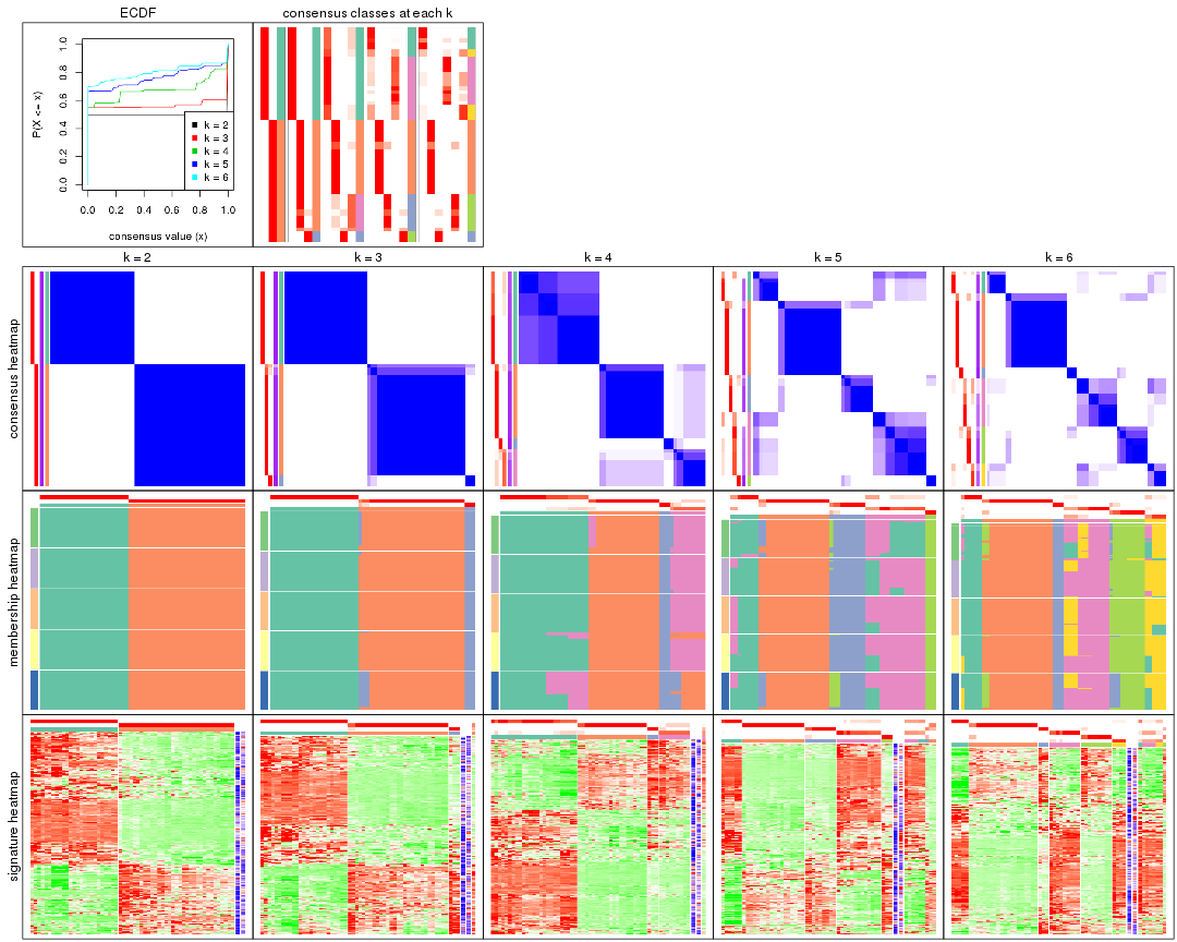
The plots are:
k and the heatmap of
predicted classes for each k.k.k.k.All the plots in panels can be made by individual functions and they are plotted later in this section.
select_partition_number() produces several plots showing different
statistics for choosing “optimized” k. There are following statistics:
k;k, the area increased is defined as \(A_k - A_{k-1}\).The detailed explanations of these statistics can be found in the cola vignette.
Generally speaking, lower PAC score, higher mean silhouette score or higher
concordance corresponds to better partition. Rand index and Jaccard index
measure how similar the current partition is compared to partition with k-1.
If they are too similar, we won't accept k is better than k-1.
select_partition_number(res)
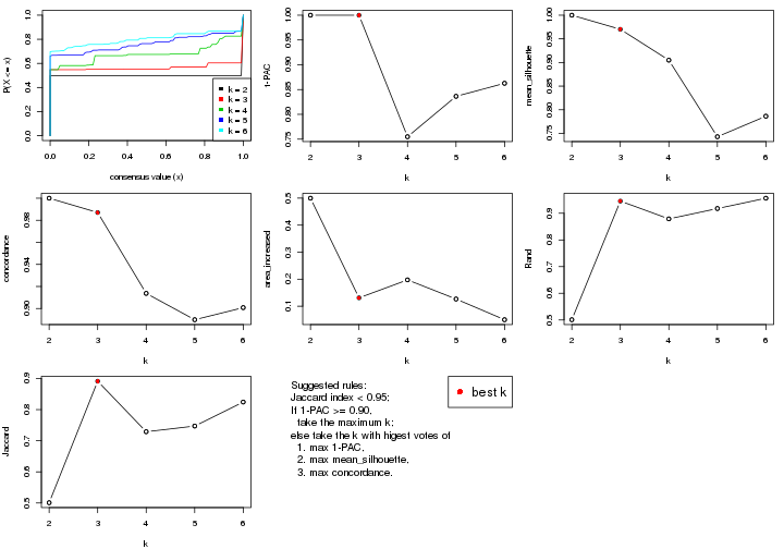
The numeric values for all these statistics can be obtained by get_stats().
get_stats(res)
#>   k 1-PAC mean_silhouette concordance area_increased  Rand Jaccard
#> 2 2 1.000           1.000       1.000         0.4996 0.501   0.501
#> 3 3 1.000           0.970       0.987         0.1311 0.946   0.891
#> 4 4 0.755           0.905       0.914         0.1975 0.879   0.729
#> 5 5 0.836           0.743       0.890         0.1267 0.918   0.747
#> 6 6 0.863           0.786       0.901         0.0501 0.956   0.824
suggest_best_k() suggests the best \(k\) based on these statistics. The rules are as follows:
suggest_best_k(res)
#> [1] 3
#> attr(,"optional")
#> [1] 2
There is also optional best \(k\) = 2 that is worth to check.
Following shows the table of the partitions (You need to click the show/hide
code output link to see it). The membership matrix (columns with name p*)
is inferred by
clue::cl_consensus()
function with the SE method. Basically the value in the membership matrix
represents the probability to belong to a certain group. The finall class
label for an item is determined with the group with highest probability it
belongs to.
In get_classes() function, the entropy is calculated from the membership
matrix and the silhouette score is calculated from the consensus matrix.
cbind(get_classes(res, k = 2), get_membership(res, k = 2))
#>           class entropy silhouette p1 p2
#> ERR789082     2       0          1  0  1
#> ERR789083     2       0          1  0  1
#> ERR789191     2       0          1  0  1
#> ERR789192     2       0          1  0  1
#> ERR789213     1       0          1  1  0
#> ERR789385     1       0          1  1  0
#> ERR789393     1       0          1  1  0
#> ERR789394     1       0          1  1  0
#> ERR789193     2       0          1  0  1
#> ERR789194     2       0          1  0  1
#> ERR789195     2       0          1  0  1
#> ERR789196     2       0          1  0  1
#> ERR789388     1       0          1  1  0
#> ERR789197     2       0          1  0  1
#> ERR789198     2       0          1  0  1
#> ERR789214     1       0          1  1  0
#> ERR789397     1       0          1  1  0
#> ERR789398     1       0          1  1  0
#> ERR789199     2       0          1  0  1
#> ERR789200     2       0          1  0  1
#> ERR789201     2       0          1  0  1
#> ERR789202     2       0          1  0  1
#> ERR789215     1       0          1  1  0
#> ERR789203     2       0          1  0  1
#> ERR789204     2       0          1  0  1
#> ERR789383     1       0          1  1  0
#> ERR789205     2       0          1  0  1
#> ERR789206     2       0          1  0  1
#> ERR789399     1       0          1  1  0
#> ERR789400     1       0          1  1  0
#> ERR789207     2       0          1  0  1
#> ERR789208     2       0          1  0  1
#> ERR789209     2       0          1  0  1
#> ERR789210     2       0          1  0  1
#> ERR789211     2       0          1  0  1
#> ERR789212     2       0          1  0  1
#> ERR789386     1       0          1  1  0
#> ERR789076     2       0          1  0  1
#> ERR789077     2       0          1  0  1
#> ERR789384     1       0          1  1  0
#> ERR789078     2       0          1  0  1
#> ERR789079     2       0          1  0  1
#> ERR789216     1       0          1  1  0
#> ERR789080     2       0          1  0  1
#> ERR789387     1       0          1  1  0
#> ERR789081     2       0          1  0  1
#> ERR789064     2       0          1  0  1
#> ERR779485     2       0          1  0  1
#> ERR789065     2       0          1  0  1
#> ERR789401     1       0          1  1  0
#> ERR789402     1       0          1  1  0
#> ERR789403     1       0          1  1  0
#> ERR789389     1       0          1  1  0
#> ERR789395     1       0          1  1  0
#> ERR789396     1       0          1  1  0
#> ERR789390     1       0          1  1  0
#> ERR789391     1       0          1  1  0
#> ERR789392     1       0          1  1  0
cbind(get_classes(res, k = 3), get_membership(res, k = 3))
#>           class entropy silhouette p1    p2    p3
#> ERR789082     2   0.000      0.974  0 1.000 0.000
#> ERR789083     2   0.000      0.974  0 1.000 0.000
#> ERR789191     2   0.000      0.974  0 1.000 0.000
#> ERR789192     2   0.000      0.974  0 1.000 0.000
#> ERR789213     1   0.000      1.000  1 0.000 0.000
#> ERR789385     1   0.000      1.000  1 0.000 0.000
#> ERR789393     1   0.000      1.000  1 0.000 0.000
#> ERR789394     1   0.000      1.000  1 0.000 0.000
#> ERR789193     3   0.000      1.000  0 0.000 1.000
#> ERR789194     3   0.000      1.000  0 0.000 1.000
#> ERR789195     2   0.000      0.974  0 1.000 0.000
#> ERR789196     2   0.000      0.974  0 1.000 0.000
#> ERR789388     1   0.000      1.000  1 0.000 0.000
#> ERR789197     2   0.000      0.974  0 1.000 0.000
#> ERR789198     2   0.000      0.974  0 1.000 0.000
#> ERR789214     1   0.000      1.000  1 0.000 0.000
#> ERR789397     1   0.000      1.000  1 0.000 0.000
#> ERR789398     1   0.000      1.000  1 0.000 0.000
#> ERR789199     2   0.000      0.974  0 1.000 0.000
#> ERR789200     2   0.000      0.974  0 1.000 0.000
#> ERR789201     2   0.000      0.974  0 1.000 0.000
#> ERR789202     2   0.000      0.974  0 1.000 0.000
#> ERR789215     1   0.000      1.000  1 0.000 0.000
#> ERR789203     2   0.440      0.774  0 0.812 0.188
#> ERR789204     2   0.440      0.774  0 0.812 0.188
#> ERR789383     1   0.000      1.000  1 0.000 0.000
#> ERR789205     2   0.000      0.974  0 1.000 0.000
#> ERR789206     2   0.000      0.974  0 1.000 0.000
#> ERR789399     1   0.000      1.000  1 0.000 0.000
#> ERR789400     1   0.000      1.000  1 0.000 0.000
#> ERR789207     2   0.000      0.974  0 1.000 0.000
#> ERR789208     2   0.000      0.974  0 1.000 0.000
#> ERR789209     2   0.000      0.974  0 1.000 0.000
#> ERR789210     2   0.000      0.974  0 1.000 0.000
#> ERR789211     2   0.000      0.974  0 1.000 0.000
#> ERR789212     2   0.000      0.974  0 1.000 0.000
#> ERR789386     1   0.000      1.000  1 0.000 0.000
#> ERR789076     2   0.000      0.974  0 1.000 0.000
#> ERR789077     2   0.000      0.974  0 1.000 0.000
#> ERR789384     1   0.000      1.000  1 0.000 0.000
#> ERR789078     2   0.000      0.974  0 1.000 0.000
#> ERR789079     2   0.000      0.974  0 1.000 0.000
#> ERR789216     1   0.000      1.000  1 0.000 0.000
#> ERR789080     2   0.000      0.974  0 1.000 0.000
#> ERR789387     1   0.000      1.000  1 0.000 0.000
#> ERR789081     2   0.000      0.974  0 1.000 0.000
#> ERR789064     2   0.000      0.974  0 1.000 0.000
#> ERR779485     3   0.000      1.000  0 0.000 1.000
#> ERR789065     2   0.603      0.435  0 0.624 0.376
#> ERR789401     1   0.000      1.000  1 0.000 0.000
#> ERR789402     1   0.000      1.000  1 0.000 0.000
#> ERR789403     1   0.000      1.000  1 0.000 0.000
#> ERR789389     1   0.000      1.000  1 0.000 0.000
#> ERR789395     1   0.000      1.000  1 0.000 0.000
#> ERR789396     1   0.000      1.000  1 0.000 0.000
#> ERR789390     1   0.000      1.000  1 0.000 0.000
#> ERR789391     1   0.000      1.000  1 0.000 0.000
#> ERR789392     1   0.000      1.000  1 0.000 0.000
cbind(get_classes(res, k = 4), get_membership(res, k = 4))
#>           class entropy silhouette    p1    p2    p3    p4
#> ERR789082     2   0.000      0.978 0.000 1.000 0.000 0.000
#> ERR789083     2   0.000      0.978 0.000 1.000 0.000 0.000
#> ERR789191     2   0.000      0.978 0.000 1.000 0.000 0.000
#> ERR789192     2   0.000      0.978 0.000 1.000 0.000 0.000
#> ERR789213     1   0.000      0.916 1.000 0.000 0.000 0.000
#> ERR789385     1   0.000      0.916 1.000 0.000 0.000 0.000
#> ERR789393     1   0.000      0.916 1.000 0.000 0.000 0.000
#> ERR789394     1   0.000      0.916 1.000 0.000 0.000 0.000
#> ERR789193     3   0.000      1.000 0.000 0.000 1.000 0.000
#> ERR789194     3   0.000      1.000 0.000 0.000 1.000 0.000
#> ERR789195     4   0.391      0.881 0.000 0.232 0.000 0.768
#> ERR789196     4   0.391      0.881 0.000 0.232 0.000 0.768
#> ERR789388     1   0.000      0.916 1.000 0.000 0.000 0.000
#> ERR789197     4   0.391      0.881 0.000 0.232 0.000 0.768
#> ERR789198     4   0.391      0.881 0.000 0.232 0.000 0.768
#> ERR789214     1   0.000      0.916 1.000 0.000 0.000 0.000
#> ERR789397     1   0.000      0.916 1.000 0.000 0.000 0.000
#> ERR789398     1   0.000      0.916 1.000 0.000 0.000 0.000
#> ERR789199     2   0.000      0.978 0.000 1.000 0.000 0.000
#> ERR789200     2   0.000      0.978 0.000 1.000 0.000 0.000
#> ERR789201     2   0.327      0.754 0.000 0.832 0.000 0.168
#> ERR789202     2   0.327      0.754 0.000 0.832 0.000 0.168
#> ERR789215     1   0.276      0.903 0.872 0.000 0.000 0.128
#> ERR789203     4   0.472      0.679 0.000 0.044 0.188 0.768
#> ERR789204     4   0.472      0.679 0.000 0.044 0.188 0.768
#> ERR789383     1   0.276      0.903 0.872 0.000 0.000 0.128
#> ERR789205     4   0.391      0.881 0.000 0.232 0.000 0.768
#> ERR789206     4   0.391      0.881 0.000 0.232 0.000 0.768
#> ERR789399     1   0.276      0.903 0.872 0.000 0.000 0.128
#> ERR789400     1   0.276      0.903 0.872 0.000 0.000 0.128
#> ERR789207     2   0.000      0.978 0.000 1.000 0.000 0.000
#> ERR789208     2   0.000      0.978 0.000 1.000 0.000 0.000
#> ERR789209     2   0.000      0.978 0.000 1.000 0.000 0.000
#> ERR789210     2   0.000      0.978 0.000 1.000 0.000 0.000
#> ERR789211     2   0.000      0.978 0.000 1.000 0.000 0.000
#> ERR789212     2   0.000      0.978 0.000 1.000 0.000 0.000
#> ERR789386     1   0.000      0.916 1.000 0.000 0.000 0.000
#> ERR789076     4   0.391      0.881 0.000 0.232 0.000 0.768
#> ERR789077     2   0.000      0.978 0.000 1.000 0.000 0.000
#> ERR789384     1   0.000      0.916 1.000 0.000 0.000 0.000
#> ERR789078     2   0.000      0.978 0.000 1.000 0.000 0.000
#> ERR789079     2   0.000      0.978 0.000 1.000 0.000 0.000
#> ERR789216     1   0.000      0.916 1.000 0.000 0.000 0.000
#> ERR789080     2   0.000      0.978 0.000 1.000 0.000 0.000
#> ERR789387     1   0.000      0.916 1.000 0.000 0.000 0.000
#> ERR789081     2   0.000      0.978 0.000 1.000 0.000 0.000
#> ERR789064     2   0.000      0.978 0.000 1.000 0.000 0.000
#> ERR779485     3   0.000      1.000 0.000 0.000 1.000 0.000
#> ERR789065     4   0.592      0.391 0.000 0.044 0.376 0.580
#> ERR789401     1   0.391      0.855 0.768 0.000 0.000 0.232
#> ERR789402     1   0.391      0.855 0.768 0.000 0.000 0.232
#> ERR789403     1   0.391      0.855 0.768 0.000 0.000 0.232
#> ERR789389     1   0.384      0.859 0.776 0.000 0.000 0.224
#> ERR789395     1   0.391      0.855 0.768 0.000 0.000 0.232
#> ERR789396     1   0.391      0.855 0.768 0.000 0.000 0.232
#> ERR789390     1   0.281      0.902 0.868 0.000 0.000 0.132
#> ERR789391     1   0.281      0.902 0.868 0.000 0.000 0.132
#> ERR789392     1   0.000      0.916 1.000 0.000 0.000 0.000
cbind(get_classes(res, k = 5), get_membership(res, k = 5))
#>           class entropy silhouette    p1    p2    p3    p4    p5
#> ERR789082     2   0.000     0.9582 0.000 1.000 0.000 0.000 0.000
#> ERR789083     2   0.000     0.9582 0.000 1.000 0.000 0.000 0.000
#> ERR789191     2   0.000     0.9582 0.000 1.000 0.000 0.000 0.000
#> ERR789192     2   0.000     0.9582 0.000 1.000 0.000 0.000 0.000
#> ERR789213     4   0.277     0.7330 0.164 0.000 0.000 0.836 0.000
#> ERR789385     4   0.277     0.7330 0.164 0.000 0.000 0.836 0.000
#> ERR789393     4   0.277     0.7330 0.164 0.000 0.000 0.836 0.000
#> ERR789394     4   0.277     0.7330 0.164 0.000 0.000 0.836 0.000
#> ERR789193     5   0.000     1.0000 0.000 0.000 0.000 0.000 1.000
#> ERR789194     5   0.000     1.0000 0.000 0.000 0.000 0.000 1.000
#> ERR789195     3   0.000     0.9066 0.000 0.000 1.000 0.000 0.000
#> ERR789196     3   0.000     0.9066 0.000 0.000 1.000 0.000 0.000
#> ERR789388     4   0.318     0.7177 0.208 0.000 0.000 0.792 0.000
#> ERR789197     3   0.000     0.9066 0.000 0.000 1.000 0.000 0.000
#> ERR789198     3   0.000     0.9066 0.000 0.000 1.000 0.000 0.000
#> ERR789214     4   0.318     0.7177 0.208 0.000 0.000 0.792 0.000
#> ERR789397     4   0.318     0.7177 0.208 0.000 0.000 0.792 0.000
#> ERR789398     4   0.318     0.7177 0.208 0.000 0.000 0.792 0.000
#> ERR789199     2   0.000     0.9582 0.000 1.000 0.000 0.000 0.000
#> ERR789200     2   0.000     0.9582 0.000 1.000 0.000 0.000 0.000
#> ERR789201     2   0.405     0.4983 0.000 0.644 0.356 0.000 0.000
#> ERR789202     2   0.405     0.4983 0.000 0.644 0.356 0.000 0.000
#> ERR789215     4   0.429    -0.0655 0.468 0.000 0.000 0.532 0.000
#> ERR789203     3   0.300     0.7738 0.000 0.000 0.812 0.000 0.188
#> ERR789204     3   0.300     0.7738 0.000 0.000 0.812 0.000 0.188
#> ERR789383     4   0.429    -0.0655 0.468 0.000 0.000 0.532 0.000
#> ERR789205     3   0.000     0.9066 0.000 0.000 1.000 0.000 0.000
#> ERR789206     3   0.000     0.9066 0.000 0.000 1.000 0.000 0.000
#> ERR789399     4   0.429    -0.0655 0.468 0.000 0.000 0.532 0.000
#> ERR789400     4   0.429    -0.0655 0.468 0.000 0.000 0.532 0.000
#> ERR789207     2   0.000     0.9582 0.000 1.000 0.000 0.000 0.000
#> ERR789208     2   0.000     0.9582 0.000 1.000 0.000 0.000 0.000
#> ERR789209     2   0.000     0.9582 0.000 1.000 0.000 0.000 0.000
#> ERR789210     2   0.000     0.9582 0.000 1.000 0.000 0.000 0.000
#> ERR789211     2   0.000     0.9582 0.000 1.000 0.000 0.000 0.000
#> ERR789212     2   0.000     0.9582 0.000 1.000 0.000 0.000 0.000
#> ERR789386     4   0.029     0.6500 0.008 0.000 0.000 0.992 0.000
#> ERR789076     3   0.000     0.9066 0.000 0.000 1.000 0.000 0.000
#> ERR789077     2   0.000     0.9582 0.000 1.000 0.000 0.000 0.000
#> ERR789384     4   0.277     0.7330 0.164 0.000 0.000 0.836 0.000
#> ERR789078     2   0.000     0.9582 0.000 1.000 0.000 0.000 0.000
#> ERR789079     2   0.000     0.9582 0.000 1.000 0.000 0.000 0.000
#> ERR789216     4   0.000     0.6564 0.000 0.000 0.000 1.000 0.000
#> ERR789080     2   0.000     0.9582 0.000 1.000 0.000 0.000 0.000
#> ERR789387     4   0.000     0.6564 0.000 0.000 0.000 1.000 0.000
#> ERR789081     2   0.000     0.9582 0.000 1.000 0.000 0.000 0.000
#> ERR789064     2   0.000     0.9582 0.000 1.000 0.000 0.000 0.000
#> ERR779485     5   0.000     1.0000 0.000 0.000 0.000 0.000 1.000
#> ERR789065     3   0.411     0.4641 0.000 0.000 0.624 0.000 0.376
#> ERR789401     1   0.029     0.7988 0.992 0.000 0.000 0.008 0.000
#> ERR789402     1   0.029     0.7988 0.992 0.000 0.000 0.008 0.000
#> ERR789403     1   0.029     0.7988 0.992 0.000 0.000 0.008 0.000
#> ERR789389     1   0.112     0.7739 0.956 0.000 0.000 0.044 0.000
#> ERR789395     1   0.029     0.7988 0.992 0.000 0.000 0.008 0.000
#> ERR789396     1   0.029     0.7988 0.992 0.000 0.000 0.008 0.000
#> ERR789390     1   0.430    -0.1229 0.528 0.000 0.000 0.472 0.000
#> ERR789391     1   0.430    -0.1229 0.528 0.000 0.000 0.472 0.000
#> ERR789392     4   0.277     0.7330 0.164 0.000 0.000 0.836 0.000
cbind(get_classes(res, k = 6), get_membership(res, k = 6))
#>           class entropy silhouette    p1    p2    p3    p4    p5    p6
#> ERR789082     2   0.000      0.958 0.000 1.000 0.000 0.000 0.000 0.000
#> ERR789083     2   0.000      0.958 0.000 1.000 0.000 0.000 0.000 0.000
#> ERR789191     2   0.000      0.958 0.000 1.000 0.000 0.000 0.000 0.000
#> ERR789192     2   0.000      0.958 0.000 1.000 0.000 0.000 0.000 0.000
#> ERR789213     4   0.000      0.724 0.000 0.000 0.000 1.000 0.000 0.000
#> ERR789385     4   0.000      0.724 0.000 0.000 0.000 1.000 0.000 0.000
#> ERR789393     4   0.000      0.724 0.000 0.000 0.000 1.000 0.000 0.000
#> ERR789394     4   0.000      0.724 0.000 0.000 0.000 1.000 0.000 0.000
#> ERR789193     3   0.000      1.000 0.000 0.000 1.000 0.000 0.000 0.000
#> ERR789194     3   0.000      1.000 0.000 0.000 1.000 0.000 0.000 0.000
#> ERR789195     5   0.000      0.904 0.000 0.000 0.000 0.000 1.000 0.000
#> ERR789196     5   0.000      0.904 0.000 0.000 0.000 0.000 1.000 0.000
#> ERR789388     4   0.519      0.142 0.088 0.000 0.000 0.464 0.000 0.448
#> ERR789197     5   0.000      0.904 0.000 0.000 0.000 0.000 1.000 0.000
#> ERR789198     5   0.000      0.904 0.000 0.000 0.000 0.000 1.000 0.000
#> ERR789214     4   0.519      0.142 0.088 0.000 0.000 0.464 0.000 0.448
#> ERR789397     4   0.519      0.142 0.088 0.000 0.000 0.464 0.000 0.448
#> ERR789398     4   0.519      0.142 0.088 0.000 0.000 0.464 0.000 0.448
#> ERR789199     2   0.000      0.958 0.000 1.000 0.000 0.000 0.000 0.000
#> ERR789200     2   0.000      0.958 0.000 1.000 0.000 0.000 0.000 0.000
#> ERR789201     2   0.385      0.501 0.000 0.644 0.000 0.000 0.348 0.008
#> ERR789202     2   0.385      0.501 0.000 0.644 0.000 0.000 0.348 0.008
#> ERR789215     6   0.144      0.785 0.072 0.000 0.000 0.000 0.000 0.928
#> ERR789203     5   0.295      0.772 0.000 0.000 0.188 0.000 0.804 0.008
#> ERR789204     5   0.295      0.772 0.000 0.000 0.188 0.000 0.804 0.008
#> ERR789383     6   0.144      0.785 0.072 0.000 0.000 0.000 0.000 0.928
#> ERR789205     5   0.026      0.902 0.000 0.000 0.000 0.000 0.992 0.008
#> ERR789206     5   0.026      0.902 0.000 0.000 0.000 0.000 0.992 0.008
#> ERR789399     6   0.144      0.785 0.072 0.000 0.000 0.000 0.000 0.928
#> ERR789400     6   0.144      0.785 0.072 0.000 0.000 0.000 0.000 0.928
#> ERR789207     2   0.000      0.958 0.000 1.000 0.000 0.000 0.000 0.000
#> ERR789208     2   0.000      0.958 0.000 1.000 0.000 0.000 0.000 0.000
#> ERR789209     2   0.000      0.958 0.000 1.000 0.000 0.000 0.000 0.000
#> ERR789210     2   0.000      0.958 0.000 1.000 0.000 0.000 0.000 0.000
#> ERR789211     2   0.000      0.958 0.000 1.000 0.000 0.000 0.000 0.000
#> ERR789212     2   0.000      0.958 0.000 1.000 0.000 0.000 0.000 0.000
#> ERR789386     4   0.276      0.634 0.000 0.000 0.000 0.804 0.000 0.196
#> ERR789076     5   0.000      0.904 0.000 0.000 0.000 0.000 1.000 0.000
#> ERR789077     2   0.000      0.958 0.000 1.000 0.000 0.000 0.000 0.000
#> ERR789384     4   0.026      0.722 0.000 0.000 0.000 0.992 0.000 0.008
#> ERR789078     2   0.000      0.958 0.000 1.000 0.000 0.000 0.000 0.000
#> ERR789079     2   0.000      0.958 0.000 1.000 0.000 0.000 0.000 0.000
#> ERR789216     4   0.270      0.641 0.000 0.000 0.000 0.812 0.000 0.188
#> ERR789080     2   0.000      0.958 0.000 1.000 0.000 0.000 0.000 0.000
#> ERR789387     4   0.270      0.641 0.000 0.000 0.000 0.812 0.000 0.188
#> ERR789081     2   0.000      0.958 0.000 1.000 0.000 0.000 0.000 0.000
#> ERR789064     2   0.000      0.958 0.000 1.000 0.000 0.000 0.000 0.000
#> ERR779485     3   0.000      1.000 0.000 0.000 1.000 0.000 0.000 0.000
#> ERR789065     5   0.370      0.468 0.000 0.000 0.376 0.000 0.624 0.000
#> ERR789401     1   0.000      0.918 1.000 0.000 0.000 0.000 0.000 0.000
#> ERR789402     1   0.000      0.918 1.000 0.000 0.000 0.000 0.000 0.000
#> ERR789403     1   0.000      0.918 1.000 0.000 0.000 0.000 0.000 0.000
#> ERR789389     1   0.510      0.485 0.628 0.000 0.000 0.156 0.000 0.216
#> ERR789395     1   0.000      0.918 1.000 0.000 0.000 0.000 0.000 0.000
#> ERR789396     1   0.000      0.918 1.000 0.000 0.000 0.000 0.000 0.000
#> ERR789390     6   0.524      0.488 0.312 0.000 0.000 0.120 0.000 0.568
#> ERR789391     6   0.524      0.488 0.312 0.000 0.000 0.120 0.000 0.568
#> ERR789392     4   0.000      0.724 0.000 0.000 0.000 1.000 0.000 0.000
Heatmaps for the consensus matrix. It visualizes the probability of two samples to be in a same group.
consensus_heatmap(res, k = 2)

consensus_heatmap(res, k = 3)
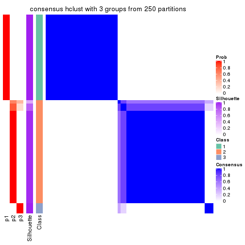
consensus_heatmap(res, k = 4)
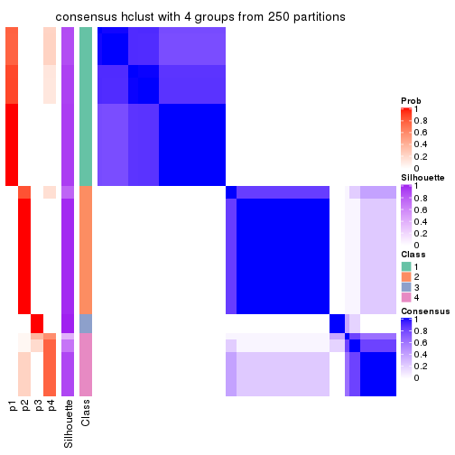
consensus_heatmap(res, k = 5)
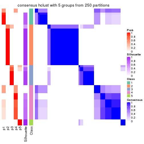
consensus_heatmap(res, k = 6)
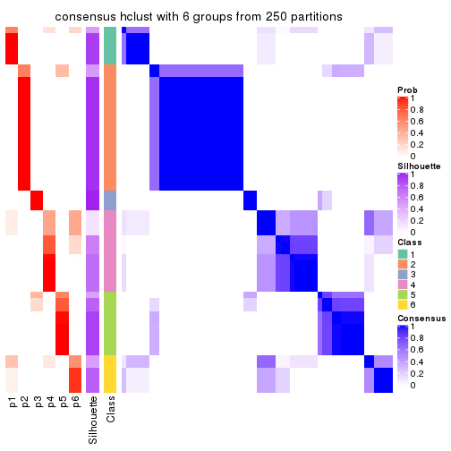
Heatmaps for the membership of samples in all partitions to see how consistent they are:
membership_heatmap(res, k = 2)

membership_heatmap(res, k = 3)
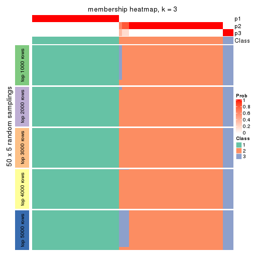
membership_heatmap(res, k = 4)
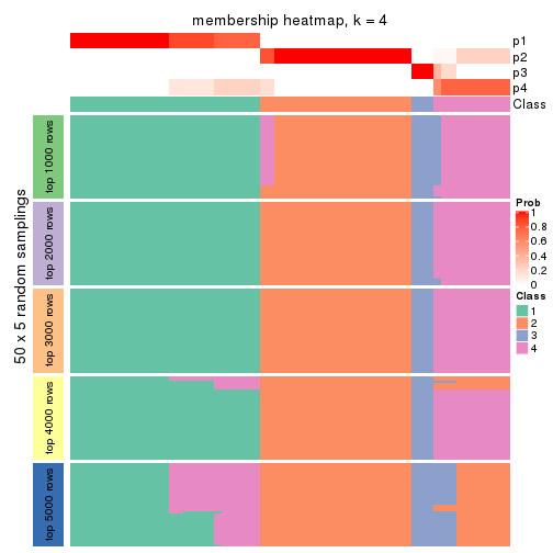
membership_heatmap(res, k = 5)
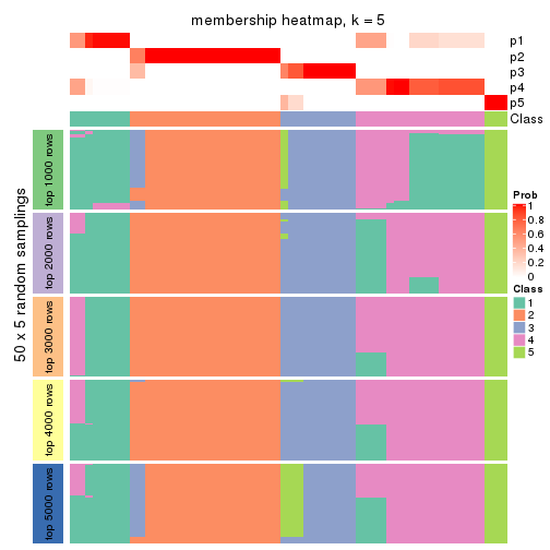
membership_heatmap(res, k = 6)
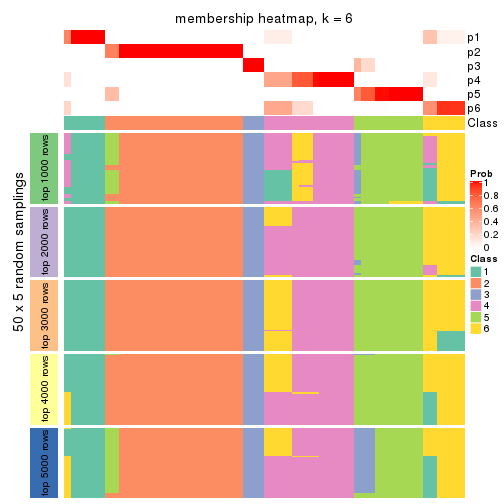
As soon as we have had the classes for columns, we can look for signatures which are significantly different between classes which can be candidate marks for certain classes. Following are the heatmaps for signatures.
Signature heatmaps where rows are scaled:
get_signatures(res, k = 2)

get_signatures(res, k = 3)
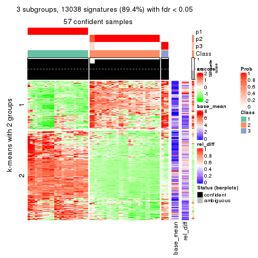
get_signatures(res, k = 4)
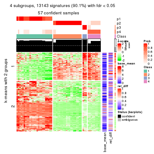
get_signatures(res, k = 5)
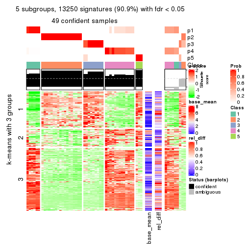
get_signatures(res, k = 6)
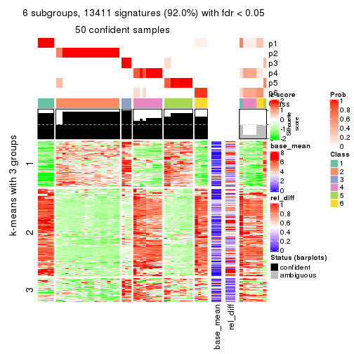
Signature heatmaps where rows are not scaled:
get_signatures(res, k = 2, scale_rows = FALSE)

get_signatures(res, k = 3, scale_rows = FALSE)
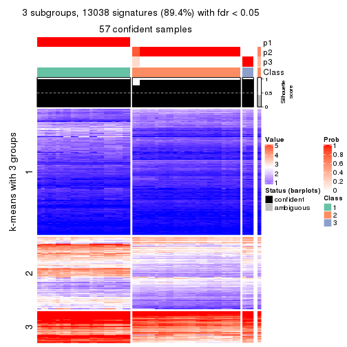
get_signatures(res, k = 4, scale_rows = FALSE)
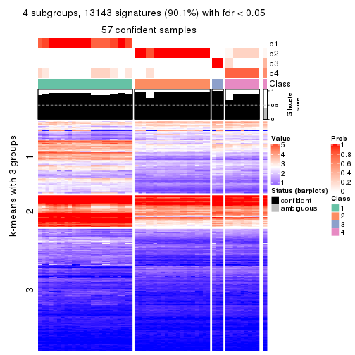
get_signatures(res, k = 5, scale_rows = FALSE)
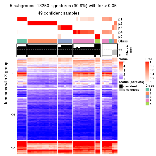
get_signatures(res, k = 6, scale_rows = FALSE)
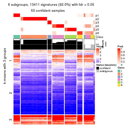
Compare the overlap of signatures from different k:
compare_signatures(res)
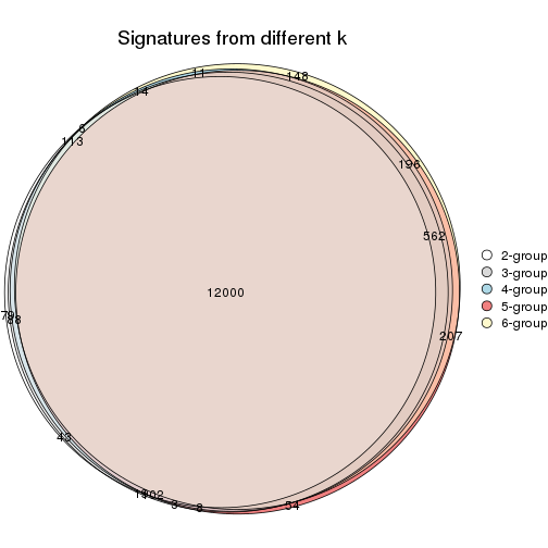
get_signature() returns a data frame invisibly. TO get the list of signatures, the function
call should be assigned to a variable explicitly. In following code, if plot argument is set
to FALSE, no heatmap is plotted while only the differential analysis is performed.
# code only for demonstration
tb = get_signature(res, k = ..., plot = FALSE)
An example of the output of tb is:
#>   which_row         fdr    mean_1    mean_2 scaled_mean_1 scaled_mean_2 km
#> 1        38 0.042760348  8.373488  9.131774    -0.5533452     0.5164555  1
#> 2        40 0.018707592  7.106213  8.469186    -0.6173731     0.5762149  1
#> 3        55 0.019134737 10.221463 11.207825    -0.6159697     0.5749050  1
#> 4        59 0.006059896  5.921854  7.869574    -0.6899429     0.6439467  1
#> 5        60 0.018055526  8.928898 10.211722    -0.6204761     0.5791110  1
#> 6        98 0.009384629 15.714769 14.887706     0.6635654    -0.6193277  2
...
The columns in tb are:
which_row: row indices corresponding to the input matrix.fdr: FDR for the differential test. mean_x: The mean value in group x.scaled_mean_x: The mean value in group x after rows are scaled.km: Row groups if k-means clustering is applied to rows.UMAP plot which shows how samples are separated.
dimension_reduction(res, k = 2, method = "UMAP")

dimension_reduction(res, k = 3, method = "UMAP")

dimension_reduction(res, k = 4, method = "UMAP")
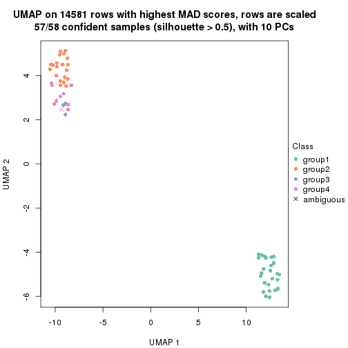
dimension_reduction(res, k = 5, method = "UMAP")
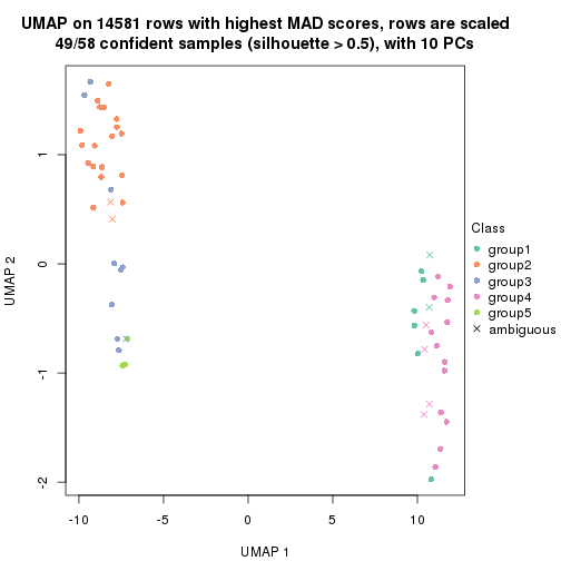
dimension_reduction(res, k = 6, method = "UMAP")
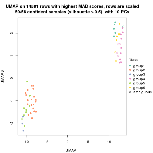
Following heatmap shows how subgroups are split when increasing k:
collect_classes(res)
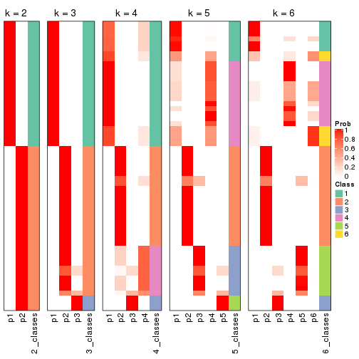
If matrix rows can be associated to genes, consider to use functional_enrichment(res,
...) to perform function enrichment for the signature genes. See this vignette for more detailed explanations.
The object with results only for a single top-value method and a single partition method can be extracted as:
res = res_list["MAD", "kmeans"]
# you can also extract it by
# res = res_list["MAD:kmeans"]
A summary of res and all the functions that can be applied to it:
res
#> A 'ConsensusPartition' object with k = 2, 3, 4, 5, 6.
#>   On a matrix with 14581 rows and 58 columns.
#>   Top rows (1000, 2000, 3000, 4000, 5000) are extracted by 'MAD' method.
#>   Subgroups are detected by 'kmeans' method.
#>   Performed in total 1250 partitions by row resampling.
#>   Best k for subgroups seems to be 2.
#>
#> Following methods can be applied to this 'ConsensusPartition' object:
#>  [1] "cola_report"             "collect_classes"         "collect_plots"
#>  [4] "collect_stats"           "colnames"                "compare_signatures"
#>  [7] "consensus_heatmap"       "dimension_reduction"     "functional_enrichment"
#> [10] "get_anno_col"            "get_anno"                "get_classes"
#> [13] "get_consensus"           "get_matrix"              "get_membership"
#> [16] "get_param"               "get_signatures"          "get_stats"
#> [19] "is_best_k"               "is_stable_k"             "membership_heatmap"
#> [22] "ncol"                    "nrow"                    "plot_ecdf"
#> [25] "rownames"                "select_partition_number" "show"
#> [28] "suggest_best_k"          "test_to_known_factors"
collect_plots() function collects all the plots made from res for all k (number of partitions)
into one single page to provide an easy and fast comparison between different k.
collect_plots(res)
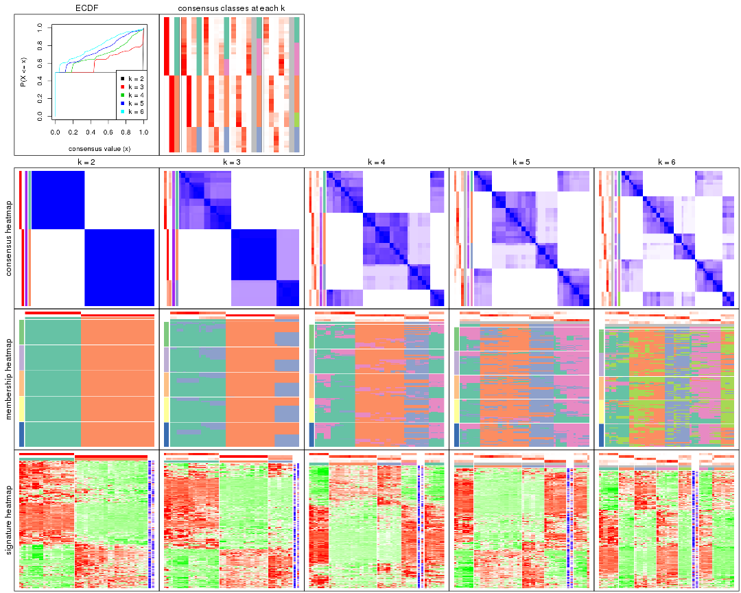
The plots are:
k and the heatmap of
predicted classes for each k.k.k.k.All the plots in panels can be made by individual functions and they are plotted later in this section.
select_partition_number() produces several plots showing different
statistics for choosing “optimized” k. There are following statistics:
k;k, the area increased is defined as \(A_k - A_{k-1}\).The detailed explanations of these statistics can be found in the cola vignette.
Generally speaking, lower PAC score, higher mean silhouette score or higher
concordance corresponds to better partition. Rand index and Jaccard index
measure how similar the current partition is compared to partition with k-1.
If they are too similar, we won't accept k is better than k-1.
select_partition_number(res)
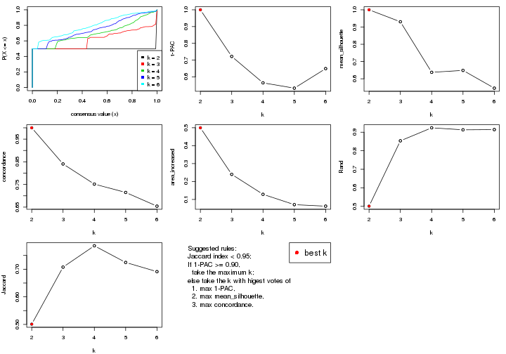
The numeric values for all these statistics can be obtained by get_stats().
get_stats(res)
#>   k 1-PAC mean_silhouette concordance area_increased  Rand Jaccard
#> 2 2 1.000           1.000       1.000         0.4996 0.501   0.501
#> 3 3 0.722           0.931       0.840         0.2399 0.854   0.708
#> 4 4 0.564           0.637       0.752         0.1286 0.924   0.785
#> 5 5 0.533           0.649       0.715         0.0710 0.913   0.725
#> 6 6 0.649           0.545       0.654         0.0625 0.914   0.691
suggest_best_k() suggests the best \(k\) based on these statistics. The rules are as follows:
suggest_best_k(res)
#> [1] 2
Following shows the table of the partitions (You need to click the show/hide
code output link to see it). The membership matrix (columns with name p*)
is inferred by
clue::cl_consensus()
function with the SE method. Basically the value in the membership matrix
represents the probability to belong to a certain group. The finall class
label for an item is determined with the group with highest probability it
belongs to.
In get_classes() function, the entropy is calculated from the membership
matrix and the silhouette score is calculated from the consensus matrix.
cbind(get_classes(res, k = 2), get_membership(res, k = 2))
#>           class entropy silhouette p1 p2
#> ERR789082     2       0          1  0  1
#> ERR789083     2       0          1  0  1
#> ERR789191     2       0          1  0  1
#> ERR789192     2       0          1  0  1
#> ERR789213     1       0          1  1  0
#> ERR789385     1       0          1  1  0
#> ERR789393     1       0          1  1  0
#> ERR789394     1       0          1  1  0
#> ERR789193     2       0          1  0  1
#> ERR789194     2       0          1  0  1
#> ERR789195     2       0          1  0  1
#> ERR789196     2       0          1  0  1
#> ERR789388     1       0          1  1  0
#> ERR789197     2       0          1  0  1
#> ERR789198     2       0          1  0  1
#> ERR789214     1       0          1  1  0
#> ERR789397     1       0          1  1  0
#> ERR789398     1       0          1  1  0
#> ERR789199     2       0          1  0  1
#> ERR789200     2       0          1  0  1
#> ERR789201     2       0          1  0  1
#> ERR789202     2       0          1  0  1
#> ERR789215     1       0          1  1  0
#> ERR789203     2       0          1  0  1
#> ERR789204     2       0          1  0  1
#> ERR789383     1       0          1  1  0
#> ERR789205     2       0          1  0  1
#> ERR789206     2       0          1  0  1
#> ERR789399     1       0          1  1  0
#> ERR789400     1       0          1  1  0
#> ERR789207     2       0          1  0  1
#> ERR789208     2       0          1  0  1
#> ERR789209     2       0          1  0  1
#> ERR789210     2       0          1  0  1
#> ERR789211     2       0          1  0  1
#> ERR789212     2       0          1  0  1
#> ERR789386     1       0          1  1  0
#> ERR789076     2       0          1  0  1
#> ERR789077     2       0          1  0  1
#> ERR789384     1       0          1  1  0
#> ERR789078     2       0          1  0  1
#> ERR789079     2       0          1  0  1
#> ERR789216     1       0          1  1  0
#> ERR789080     2       0          1  0  1
#> ERR789387     1       0          1  1  0
#> ERR789081     2       0          1  0  1
#> ERR789064     2       0          1  0  1
#> ERR779485     2       0          1  0  1
#> ERR789065     2       0          1  0  1
#> ERR789401     1       0          1  1  0
#> ERR789402     1       0          1  1  0
#> ERR789403     1       0          1  1  0
#> ERR789389     1       0          1  1  0
#> ERR789395     1       0          1  1  0
#> ERR789396     1       0          1  1  0
#> ERR789390     1       0          1  1  0
#> ERR789391     1       0          1  1  0
#> ERR789392     1       0          1  1  0
cbind(get_classes(res, k = 3), get_membership(res, k = 3))
#>           class entropy silhouette    p1    p2    p3
#> ERR789082     2  0.0000      0.999 0.000 1.000 0.000
#> ERR789083     2  0.0000      0.999 0.000 1.000 0.000
#> ERR789191     2  0.0000      0.999 0.000 1.000 0.000
#> ERR789192     2  0.0000      0.999 0.000 1.000 0.000
#> ERR789213     1  0.0424      0.850 0.992 0.000 0.008
#> ERR789385     1  0.0424      0.850 0.992 0.000 0.008
#> ERR789393     1  0.0424      0.852 0.992 0.000 0.008
#> ERR789394     1  0.0424      0.852 0.992 0.000 0.008
#> ERR789193     3  0.6244      0.991 0.000 0.440 0.560
#> ERR789194     3  0.6244      0.991 0.000 0.440 0.560
#> ERR789195     3  0.6244      0.990 0.000 0.440 0.560
#> ERR789196     3  0.6244      0.990 0.000 0.440 0.560
#> ERR789388     1  0.3686      0.865 0.860 0.000 0.140
#> ERR789197     2  0.0237      0.994 0.000 0.996 0.004
#> ERR789198     2  0.0237      0.994 0.000 0.996 0.004
#> ERR789214     1  0.0892      0.851 0.980 0.000 0.020
#> ERR789397     1  0.3551      0.865 0.868 0.000 0.132
#> ERR789398     1  0.3551      0.865 0.868 0.000 0.132
#> ERR789199     2  0.0237      0.994 0.000 0.996 0.004
#> ERR789200     2  0.0237      0.994 0.000 0.996 0.004
#> ERR789201     2  0.0000      0.999 0.000 1.000 0.000
#> ERR789202     2  0.0000      0.999 0.000 1.000 0.000
#> ERR789215     1  0.5016      0.860 0.760 0.000 0.240
#> ERR789203     3  0.6252      0.992 0.000 0.444 0.556
#> ERR789204     3  0.6252      0.992 0.000 0.444 0.556
#> ERR789383     1  0.6140      0.822 0.596 0.000 0.404
#> ERR789205     3  0.6252      0.992 0.000 0.444 0.556
#> ERR789206     3  0.6252      0.992 0.000 0.444 0.556
#> ERR789399     1  0.5810      0.846 0.664 0.000 0.336
#> ERR789400     1  0.5810      0.846 0.664 0.000 0.336
#> ERR789207     2  0.0000      0.999 0.000 1.000 0.000
#> ERR789208     2  0.0000      0.999 0.000 1.000 0.000
#> ERR789209     2  0.0000      0.999 0.000 1.000 0.000
#> ERR789210     2  0.0000      0.999 0.000 1.000 0.000
#> ERR789211     2  0.0000      0.999 0.000 1.000 0.000
#> ERR789212     2  0.0000      0.999 0.000 1.000 0.000
#> ERR789386     1  0.1163      0.849 0.972 0.000 0.028
#> ERR789076     3  0.6286      0.960 0.000 0.464 0.536
#> ERR789077     2  0.0000      0.999 0.000 1.000 0.000
#> ERR789384     1  0.0424      0.850 0.992 0.000 0.008
#> ERR789078     2  0.0000      0.999 0.000 1.000 0.000
#> ERR789079     2  0.0000      0.999 0.000 1.000 0.000
#> ERR789216     1  0.1163      0.849 0.972 0.000 0.028
#> ERR789080     2  0.0000      0.999 0.000 1.000 0.000
#> ERR789387     1  0.1163      0.849 0.972 0.000 0.028
#> ERR789081     2  0.0000      0.999 0.000 1.000 0.000
#> ERR789064     2  0.0000      0.999 0.000 1.000 0.000
#> ERR779485     3  0.6244      0.991 0.000 0.440 0.560
#> ERR789065     3  0.6244      0.991 0.000 0.440 0.560
#> ERR789401     1  0.6111      0.826 0.604 0.000 0.396
#> ERR789402     1  0.6095      0.826 0.608 0.000 0.392
#> ERR789403     1  0.6111      0.826 0.604 0.000 0.396
#> ERR789389     1  0.6062      0.830 0.616 0.000 0.384
#> ERR789395     1  0.6095      0.826 0.608 0.000 0.392
#> ERR789396     1  0.6095      0.826 0.608 0.000 0.392
#> ERR789390     1  0.5363      0.858 0.724 0.000 0.276
#> ERR789391     1  0.5363      0.858 0.724 0.000 0.276
#> ERR789392     1  0.0424      0.852 0.992 0.000 0.008
cbind(get_classes(res, k = 4), get_membership(res, k = 4))
#>           class entropy silhouette    p1    p2    p3    p4
#> ERR789082     2  0.2760      0.847 0.000 0.872 0.000 0.128
#> ERR789083     2  0.2760      0.847 0.000 0.872 0.000 0.128
#> ERR789191     2  0.3907      0.815 0.000 0.768 0.000 0.232
#> ERR789192     2  0.3907      0.815 0.000 0.768 0.000 0.232
#> ERR789213     4  0.5668      0.902 0.444 0.000 0.024 0.532
#> ERR789385     4  0.5668      0.902 0.444 0.000 0.024 0.532
#> ERR789393     4  0.6003      0.899 0.456 0.000 0.040 0.504
#> ERR789394     4  0.6003      0.899 0.456 0.000 0.040 0.504
#> ERR789193     3  0.5434      0.887 0.000 0.188 0.728 0.084
#> ERR789194     3  0.5434      0.887 0.000 0.188 0.728 0.084
#> ERR789195     3  0.4617      0.907 0.000 0.204 0.764 0.032
#> ERR789196     3  0.4617      0.907 0.000 0.204 0.764 0.032
#> ERR789388     1  0.6356     -0.230 0.596 0.000 0.084 0.320
#> ERR789197     2  0.3485      0.815 0.000 0.856 0.028 0.116
#> ERR789198     2  0.3485      0.815 0.000 0.856 0.028 0.116
#> ERR789214     1  0.6506     -0.755 0.472 0.000 0.072 0.456
#> ERR789397     1  0.6249     -0.250 0.592 0.000 0.072 0.336
#> ERR789398     1  0.6249     -0.250 0.592 0.000 0.072 0.336
#> ERR789199     2  0.3219      0.836 0.000 0.836 0.000 0.164
#> ERR789200     2  0.3219      0.836 0.000 0.836 0.000 0.164
#> ERR789201     2  0.3652      0.794 0.000 0.856 0.052 0.092
#> ERR789202     2  0.3652      0.794 0.000 0.856 0.052 0.092
#> ERR789215     1  0.5787      0.133 0.680 0.000 0.076 0.244
#> ERR789203     3  0.4387      0.909 0.000 0.200 0.776 0.024
#> ERR789204     3  0.4387      0.909 0.000 0.200 0.776 0.024
#> ERR789383     1  0.1724      0.569 0.948 0.000 0.032 0.020
#> ERR789205     3  0.5386      0.880 0.000 0.236 0.708 0.056
#> ERR789206     3  0.5386      0.880 0.000 0.236 0.708 0.056
#> ERR789399     1  0.3312      0.557 0.876 0.000 0.072 0.052
#> ERR789400     1  0.3312      0.557 0.876 0.000 0.072 0.052
#> ERR789207     2  0.1792      0.848 0.000 0.932 0.000 0.068
#> ERR789208     2  0.1792      0.848 0.000 0.932 0.000 0.068
#> ERR789209     2  0.3679      0.777 0.000 0.856 0.060 0.084
#> ERR789210     2  0.3679      0.777 0.000 0.856 0.060 0.084
#> ERR789211     2  0.2596      0.817 0.000 0.908 0.024 0.068
#> ERR789212     2  0.2596      0.817 0.000 0.908 0.024 0.068
#> ERR789386     4  0.6011      0.749 0.480 0.000 0.040 0.480
#> ERR789076     3  0.6747      0.638 0.000 0.372 0.528 0.100
#> ERR789077     2  0.3444      0.826 0.000 0.816 0.000 0.184
#> ERR789384     4  0.5590      0.848 0.456 0.000 0.020 0.524
#> ERR789078     2  0.3444      0.826 0.000 0.816 0.000 0.184
#> ERR789079     2  0.3356      0.827 0.000 0.824 0.000 0.176
#> ERR789216     1  0.6011     -0.797 0.480 0.000 0.040 0.480
#> ERR789080     2  0.3356      0.827 0.000 0.824 0.000 0.176
#> ERR789387     1  0.6011     -0.788 0.484 0.000 0.040 0.476
#> ERR789081     2  0.3356      0.827 0.000 0.824 0.000 0.176
#> ERR789064     2  0.0469      0.851 0.000 0.988 0.000 0.012
#> ERR779485     3  0.5434      0.887 0.000 0.188 0.728 0.084
#> ERR789065     3  0.4636      0.897 0.000 0.188 0.772 0.040
#> ERR789401     1  0.0921      0.580 0.972 0.000 0.028 0.000
#> ERR789402     1  0.1545      0.578 0.952 0.000 0.040 0.008
#> ERR789403     1  0.0921      0.580 0.972 0.000 0.028 0.000
#> ERR789389     1  0.1677      0.570 0.948 0.000 0.012 0.040
#> ERR789395     1  0.1545      0.578 0.952 0.000 0.040 0.008
#> ERR789396     1  0.1545      0.578 0.952 0.000 0.040 0.008
#> ERR789390     1  0.4274      0.499 0.820 0.000 0.072 0.108
#> ERR789391     1  0.4274      0.499 0.820 0.000 0.072 0.108
#> ERR789392     4  0.6003      0.899 0.456 0.000 0.040 0.504
cbind(get_classes(res, k = 5), get_membership(res, k = 5))
#>           class entropy silhouette    p1    p2    p3    p4 p5
#> ERR789082     2  0.4989      0.751 0.056 0.648 0.000 0.000 NA
#> ERR789083     2  0.4989      0.751 0.056 0.648 0.000 0.000 NA
#> ERR789191     2  0.5220      0.724 0.044 0.516 0.000 0.000 NA
#> ERR789192     2  0.5220      0.724 0.044 0.516 0.000 0.000 NA
#> ERR789213     4  0.2583      0.643 0.004 0.000 0.000 0.864 NA
#> ERR789385     4  0.2629      0.643 0.004 0.000 0.000 0.860 NA
#> ERR789393     4  0.3171      0.642 0.008 0.000 0.000 0.816 NA
#> ERR789394     4  0.3171      0.642 0.008 0.000 0.000 0.816 NA
#> ERR789193     3  0.4769      0.816 0.064 0.120 0.772 0.000 NA
#> ERR789194     3  0.4769      0.816 0.064 0.120 0.772 0.000 NA
#> ERR789195     3  0.4815      0.826 0.056 0.208 0.724 0.000 NA
#> ERR789196     3  0.4815      0.826 0.056 0.208 0.724 0.000 NA
#> ERR789388     4  0.6069      0.395 0.172 0.000 0.032 0.648 NA
#> ERR789197     2  0.5124      0.703 0.112 0.720 0.012 0.000 NA
#> ERR789198     2  0.5124      0.703 0.112 0.720 0.012 0.000 NA
#> ERR789214     4  0.3113      0.613 0.016 0.000 0.020 0.864 NA
#> ERR789397     4  0.6038      0.424 0.164 0.000 0.032 0.652 NA
#> ERR789398     4  0.6038      0.424 0.164 0.000 0.032 0.652 NA
#> ERR789199     2  0.5697      0.725 0.116 0.596 0.000 0.000 NA
#> ERR789200     2  0.5697      0.725 0.116 0.596 0.000 0.000 NA
#> ERR789201     2  0.3209      0.641 0.052 0.872 0.052 0.000 NA
#> ERR789202     2  0.3209      0.641 0.052 0.872 0.052 0.000 NA
#> ERR789215     4  0.6586     -0.223 0.308 0.000 0.032 0.540 NA
#> ERR789203     3  0.4199      0.842 0.040 0.180 0.772 0.000 NA
#> ERR789204     3  0.4199      0.842 0.040 0.180 0.772 0.000 NA
#> ERR789383     1  0.5798      0.760 0.612 0.000 0.024 0.296 NA
#> ERR789205     3  0.5230      0.806 0.064 0.268 0.660 0.000 NA
#> ERR789206     3  0.5230      0.806 0.064 0.268 0.660 0.000 NA
#> ERR789399     1  0.6942      0.608 0.476 0.000 0.044 0.356 NA
#> ERR789400     1  0.6942      0.608 0.476 0.000 0.044 0.356 NA
#> ERR789207     2  0.2890      0.744 0.004 0.836 0.000 0.000 NA
#> ERR789208     2  0.2890      0.744 0.004 0.836 0.000 0.000 NA
#> ERR789209     2  0.1770      0.649 0.008 0.936 0.048 0.000 NA
#> ERR789210     2  0.1770      0.649 0.008 0.936 0.048 0.000 NA
#> ERR789211     2  0.0324      0.692 0.004 0.992 0.000 0.000 NA
#> ERR789212     2  0.0324      0.692 0.004 0.992 0.000 0.000 NA
#> ERR789386     4  0.2170      0.625 0.020 0.000 0.020 0.924 NA
#> ERR789076     3  0.6419      0.495 0.032 0.436 0.452 0.000 NA
#> ERR789077     2  0.4440      0.710 0.004 0.528 0.000 0.000 NA
#> ERR789384     4  0.1173      0.641 0.004 0.000 0.012 0.964 NA
#> ERR789078     2  0.4440      0.710 0.004 0.528 0.000 0.000 NA
#> ERR789079     2  0.4727      0.710 0.016 0.532 0.000 0.000 NA
#> ERR789216     4  0.2170      0.625 0.020 0.000 0.020 0.924 NA
#> ERR789080     2  0.4727      0.710 0.016 0.532 0.000 0.000 NA
#> ERR789387     4  0.2249      0.622 0.020 0.000 0.020 0.920 NA
#> ERR789081     2  0.4727      0.710 0.016 0.532 0.000 0.000 NA
#> ERR789064     2  0.4031      0.762 0.044 0.772 0.000 0.000 NA
#> ERR779485     3  0.4769      0.816 0.064 0.120 0.772 0.000 NA
#> ERR789065     3  0.3554      0.830 0.024 0.120 0.836 0.000 NA
#> ERR789401     1  0.4193      0.821 0.684 0.000 0.012 0.304 NA
#> ERR789402     1  0.5460      0.810 0.620 0.000 0.024 0.316 NA
#> ERR789403     1  0.4193      0.821 0.684 0.000 0.012 0.304 NA
#> ERR789389     1  0.5600      0.767 0.584 0.000 0.016 0.348 NA
#> ERR789395     1  0.5460      0.810 0.620 0.000 0.024 0.316 NA
#> ERR789396     1  0.5460      0.810 0.620 0.000 0.024 0.316 NA
#> ERR789390     4  0.6982     -0.421 0.396 0.000 0.048 0.440 NA
#> ERR789391     4  0.6982     -0.421 0.396 0.000 0.048 0.440 NA
#> ERR789392     4  0.3171      0.642 0.008 0.000 0.000 0.816 NA
cbind(get_classes(res, k = 6), get_membership(res, k = 6))
#>           class entropy silhouette    p1    p2    p3    p4    p5 p6
#> ERR789082     2  0.4472     0.4717 0.028 0.708 0.000 0.000 0.228 NA
#> ERR789083     2  0.4472     0.4717 0.028 0.708 0.000 0.000 0.228 NA
#> ERR789191     2  0.2896     0.5723 0.028 0.868 0.000 0.000 0.076 NA
#> ERR789192     2  0.2896     0.5723 0.028 0.868 0.000 0.000 0.076 NA
#> ERR789213     4  0.0508     0.6616 0.000 0.000 0.000 0.984 0.004 NA
#> ERR789385     4  0.0000     0.6616 0.000 0.000 0.000 1.000 0.000 NA
#> ERR789393     4  0.1471     0.6563 0.000 0.000 0.000 0.932 0.004 NA
#> ERR789394     4  0.1471     0.6563 0.000 0.000 0.000 0.932 0.004 NA
#> ERR789193     3  0.5340     0.6972 0.000 0.044 0.564 0.000 0.040 NA
#> ERR789194     3  0.5340     0.6972 0.000 0.044 0.564 0.000 0.040 NA
#> ERR789195     3  0.4835     0.7334 0.016 0.048 0.748 0.000 0.120 NA
#> ERR789196     3  0.4835     0.7334 0.016 0.048 0.748 0.000 0.120 NA
#> ERR789388     4  0.6148     0.2849 0.168 0.000 0.000 0.464 0.020 NA
#> ERR789197     2  0.6546     0.0315 0.036 0.468 0.056 0.000 0.380 NA
#> ERR789198     2  0.6546     0.0315 0.036 0.468 0.056 0.000 0.380 NA
#> ERR789214     4  0.4532     0.6058 0.008 0.000 0.000 0.656 0.044 NA
#> ERR789397     4  0.5616     0.3410 0.164 0.000 0.000 0.508 0.000 NA
#> ERR789398     4  0.5616     0.3410 0.164 0.000 0.000 0.508 0.000 NA
#> ERR789199     2  0.5507     0.4412 0.048 0.620 0.000 0.000 0.256 NA
#> ERR789200     2  0.5507     0.4412 0.048 0.620 0.000 0.000 0.256 NA
#> ERR789201     5  0.6504     0.7371 0.004 0.336 0.244 0.000 0.400 NA
#> ERR789202     5  0.6504     0.7371 0.004 0.336 0.244 0.000 0.400 NA
#> ERR789215     4  0.7886    -0.2099 0.272 0.000 0.012 0.320 0.204 NA
#> ERR789203     3  0.1820     0.7512 0.000 0.044 0.928 0.000 0.012 NA
#> ERR789204     3  0.1820     0.7512 0.000 0.044 0.928 0.000 0.012 NA
#> ERR789383     1  0.6216     0.6455 0.620 0.000 0.016 0.144 0.148 NA
#> ERR789205     3  0.3066     0.6899 0.000 0.044 0.832 0.000 0.124 NA
#> ERR789206     3  0.3066     0.6899 0.000 0.044 0.832 0.000 0.124 NA
#> ERR789399     1  0.7534     0.5127 0.428 0.000 0.012 0.220 0.152 NA
#> ERR789400     1  0.7534     0.5127 0.428 0.000 0.012 0.220 0.152 NA
#> ERR789207     2  0.3756     0.0408 0.004 0.644 0.000 0.000 0.352 NA
#> ERR789208     2  0.3756     0.0408 0.004 0.644 0.000 0.000 0.352 NA
#> ERR789209     5  0.5634     0.7932 0.000 0.336 0.164 0.000 0.500 NA
#> ERR789210     5  0.5634     0.7932 0.000 0.336 0.164 0.000 0.500 NA
#> ERR789211     5  0.4892     0.6626 0.000 0.440 0.060 0.000 0.500 NA
#> ERR789212     5  0.4892     0.6626 0.000 0.440 0.060 0.000 0.500 NA
#> ERR789386     4  0.4996     0.6173 0.024 0.000 0.000 0.692 0.164 NA
#> ERR789076     3  0.6447     0.2715 0.020 0.188 0.524 0.000 0.248 NA
#> ERR789077     2  0.2190     0.5565 0.040 0.908 0.000 0.000 0.008 NA
#> ERR789384     4  0.3747     0.6503 0.000 0.000 0.000 0.784 0.112 NA
#> ERR789078     2  0.2190     0.5565 0.040 0.908 0.000 0.000 0.008 NA
#> ERR789079     2  0.2918     0.5473 0.032 0.864 0.000 0.000 0.020 NA
#> ERR789216     4  0.4996     0.6173 0.024 0.000 0.000 0.692 0.164 NA
#> ERR789080     2  0.2918     0.5473 0.032 0.864 0.000 0.000 0.020 NA
#> ERR789387     4  0.5069     0.6135 0.028 0.000 0.000 0.688 0.164 NA
#> ERR789081     2  0.2918     0.5473 0.032 0.864 0.000 0.000 0.020 NA
#> ERR789064     2  0.3934     0.3504 0.008 0.716 0.000 0.000 0.256 NA
#> ERR779485     3  0.5509     0.6972 0.004 0.044 0.564 0.000 0.044 NA
#> ERR789065     3  0.4617     0.7368 0.008 0.044 0.712 0.000 0.020 NA
#> ERR789401     1  0.2944     0.7070 0.832 0.000 0.008 0.148 0.000 NA
#> ERR789402     1  0.3800     0.7006 0.792 0.000 0.012 0.156 0.012 NA
#> ERR789403     1  0.2944     0.7070 0.832 0.000 0.008 0.148 0.000 NA
#> ERR789389     1  0.6043     0.6229 0.608 0.000 0.012 0.208 0.128 NA
#> ERR789395     1  0.3800     0.7006 0.792 0.000 0.012 0.156 0.012 NA
#> ERR789396     1  0.3800     0.7006 0.792 0.000 0.012 0.156 0.012 NA
#> ERR789390     1  0.6992     0.3102 0.372 0.000 0.008 0.336 0.044 NA
#> ERR789391     1  0.6992     0.3102 0.372 0.000 0.008 0.336 0.044 NA
#> ERR789392     4  0.1471     0.6563 0.000 0.000 0.000 0.932 0.004 NA
Heatmaps for the consensus matrix. It visualizes the probability of two samples to be in a same group.
consensus_heatmap(res, k = 2)

consensus_heatmap(res, k = 3)
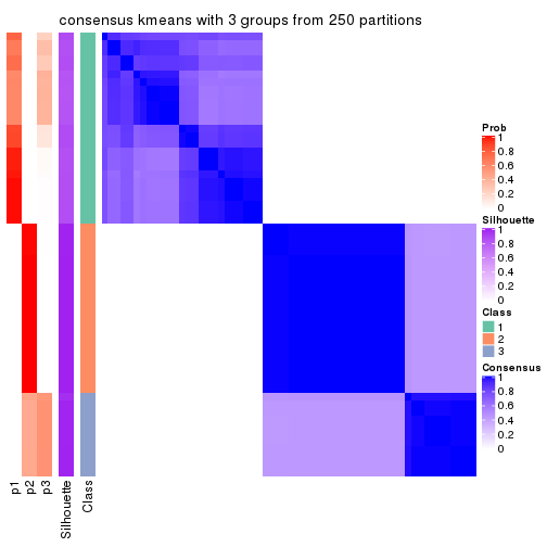
consensus_heatmap(res, k = 4)
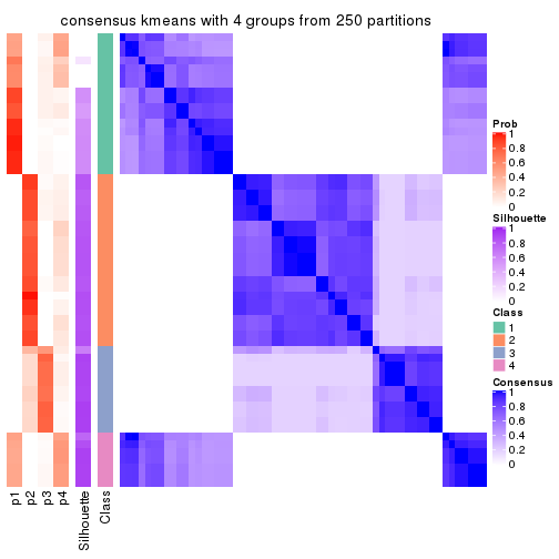
consensus_heatmap(res, k = 5)
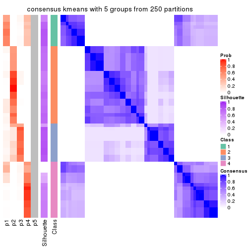
consensus_heatmap(res, k = 6)
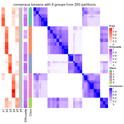
Heatmaps for the membership of samples in all partitions to see how consistent they are:
membership_heatmap(res, k = 2)

membership_heatmap(res, k = 3)
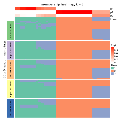
membership_heatmap(res, k = 4)
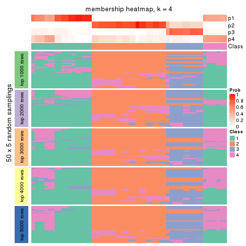
membership_heatmap(res, k = 5)
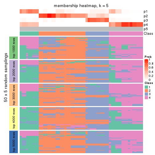
membership_heatmap(res, k = 6)
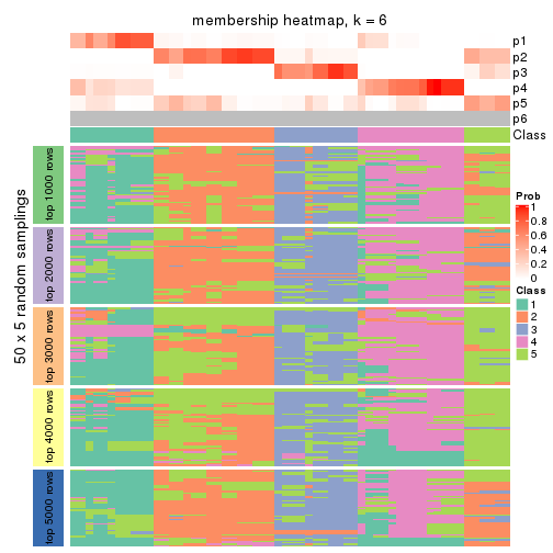
As soon as we have had the classes for columns, we can look for signatures which are significantly different between classes which can be candidate marks for certain classes. Following are the heatmaps for signatures.
Signature heatmaps where rows are scaled:
get_signatures(res, k = 2)

get_signatures(res, k = 3)
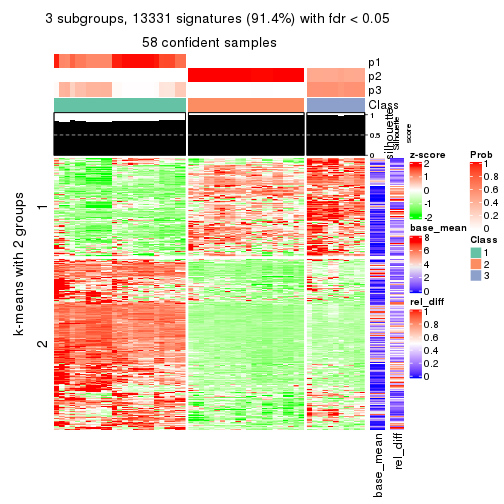
get_signatures(res, k = 4)
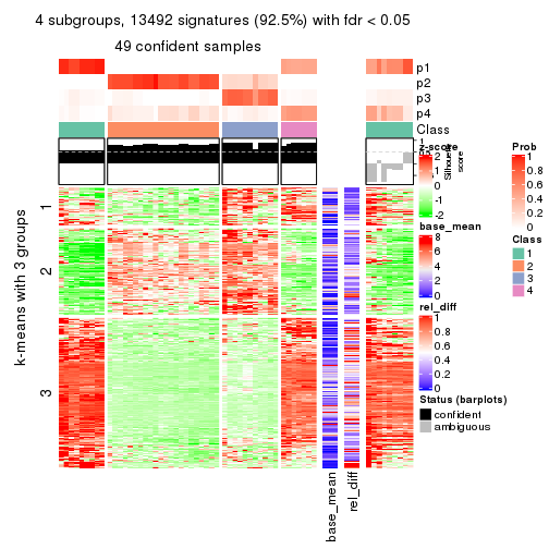
get_signatures(res, k = 5)
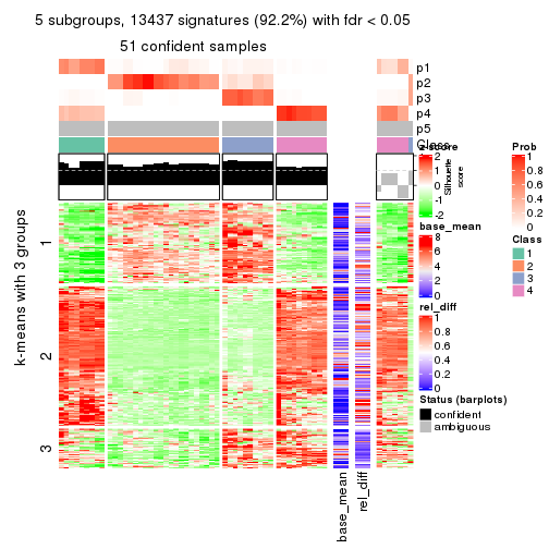
get_signatures(res, k = 6)
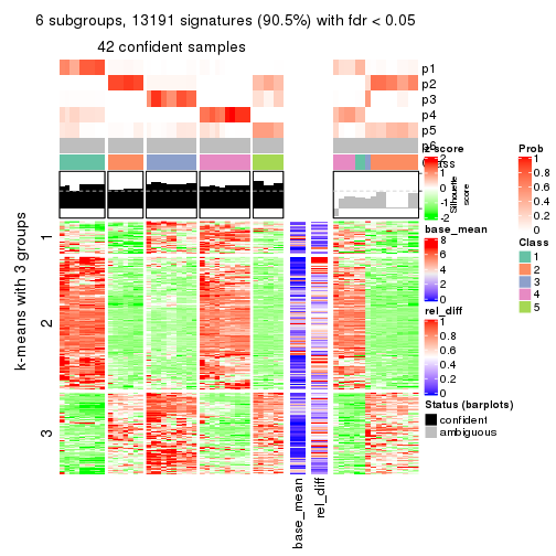
Signature heatmaps where rows are not scaled:
get_signatures(res, k = 2, scale_rows = FALSE)

get_signatures(res, k = 3, scale_rows = FALSE)
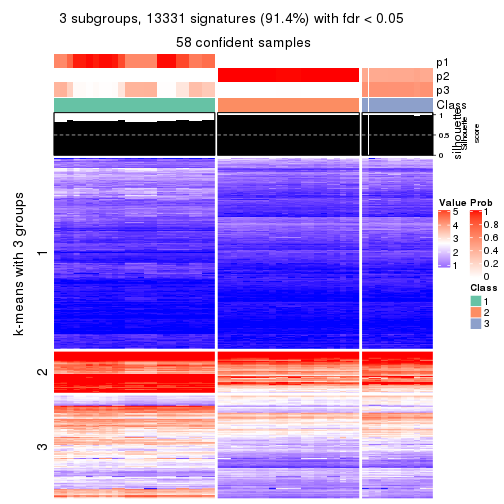
get_signatures(res, k = 4, scale_rows = FALSE)
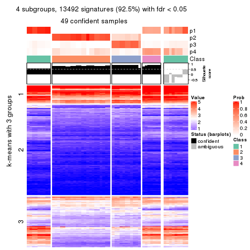
get_signatures(res, k = 5, scale_rows = FALSE)
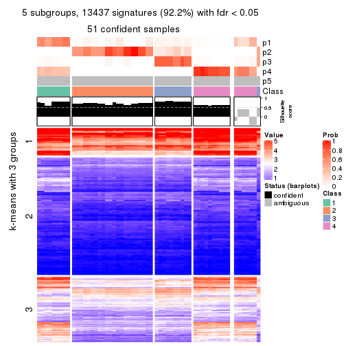
get_signatures(res, k = 6, scale_rows = FALSE)
Compare the overlap of signatures from different k:
compare_signatures(res)
get_signature() returns a data frame invisibly. TO get the list of signatures, the function
call should be assigned to a variable explicitly. In following code, if plot argument is set
to FALSE, no heatmap is plotted while only the differential analysis is performed.
# code only for demonstration
tb = get_signature(res, k = ..., plot = FALSE)
An example of the output of tb is:
#>   which_row         fdr    mean_1    mean_2 scaled_mean_1 scaled_mean_2 km
#> 1        38 0.042760348  8.373488  9.131774    -0.5533452     0.5164555  1
#> 2        40 0.018707592  7.106213  8.469186    -0.6173731     0.5762149  1
#> 3        55 0.019134737 10.221463 11.207825    -0.6159697     0.5749050  1
#> 4        59 0.006059896  5.921854  7.869574    -0.6899429     0.6439467  1
#> 5        60 0.018055526  8.928898 10.211722    -0.6204761     0.5791110  1
#> 6        98 0.009384629 15.714769 14.887706     0.6635654    -0.6193277  2
...
The columns in tb are:
which_row: row indices corresponding to the input matrix.fdr: FDR for the differential test. mean_x: The mean value in group x.scaled_mean_x: The mean value in group x after rows are scaled.km: Row groups if k-means clustering is applied to rows.UMAP plot which shows how samples are separated.
dimension_reduction(res, k = 2, method = "UMAP")

dimension_reduction(res, k = 3, method = "UMAP")
dimension_reduction(res, k = 4, method = "UMAP")

dimension_reduction(res, k = 5, method = "UMAP")
dimension_reduction(res, k = 6, method = "UMAP")
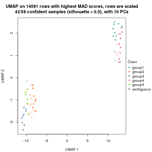
Following heatmap shows how subgroups are split when increasing k:
collect_classes(res)
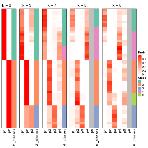
If matrix rows can be associated to genes, consider to use functional_enrichment(res,
...) to perform function enrichment for the signature genes. See this vignette for more detailed explanations.
The object with results only for a single top-value method and a single partition method can be extracted as:
res = res_list["MAD", "skmeans"]
# you can also extract it by
# res = res_list["MAD:skmeans"]
A summary of res and all the functions that can be applied to it:
res
#> A 'ConsensusPartition' object with k = 2, 3, 4, 5, 6.
#>   On a matrix with 14581 rows and 58 columns.
#>   Top rows (1000, 2000, 3000, 4000, 5000) are extracted by 'MAD' method.
#>   Subgroups are detected by 'skmeans' method.
#>   Performed in total 1250 partitions by row resampling.
#>   Best k for subgroups seems to be 3.
#>
#> Following methods can be applied to this 'ConsensusPartition' object:
#>  [1] "cola_report"             "collect_classes"         "collect_plots"
#>  [4] "collect_stats"           "colnames"                "compare_signatures"
#>  [7] "consensus_heatmap"       "dimension_reduction"     "functional_enrichment"
#> [10] "get_anno_col"            "get_anno"                "get_classes"
#> [13] "get_consensus"           "get_matrix"              "get_membership"
#> [16] "get_param"               "get_signatures"          "get_stats"
#> [19] "is_best_k"               "is_stable_k"             "membership_heatmap"
#> [22] "ncol"                    "nrow"                    "plot_ecdf"
#> [25] "rownames"                "select_partition_number" "show"
#> [28] "suggest_best_k"          "test_to_known_factors"
collect_plots() function collects all the plots made from res for all k (number of partitions)
into one single page to provide an easy and fast comparison between different k.
collect_plots(res)
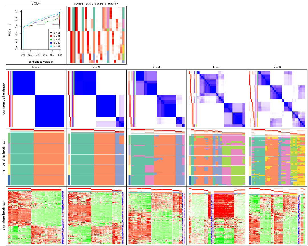
The plots are:
k and the heatmap of
predicted classes for each k.k.k.k.All the plots in panels can be made by individual functions and they are plotted later in this section.
select_partition_number() produces several plots showing different
statistics for choosing “optimized” k. There are following statistics:
k;k, the area increased is defined as \(A_k - A_{k-1}\).The detailed explanations of these statistics can be found in the cola vignette.
Generally speaking, lower PAC score, higher mean silhouette score or higher
concordance corresponds to better partition. Rand index and Jaccard index
measure how similar the current partition is compared to partition with k-1.
If they are too similar, we won't accept k is better than k-1.
select_partition_number(res)
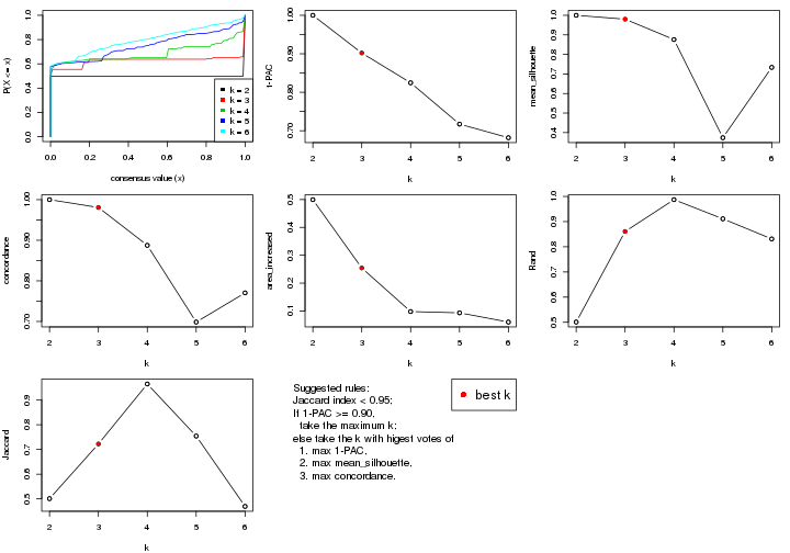
The numeric values for all these statistics can be obtained by get_stats().
get_stats(res)
#>   k 1-PAC mean_silhouette concordance area_increased  Rand Jaccard
#> 2 2 1.000           1.000       1.000         0.4996 0.501   0.501
#> 3 3 0.902           0.980       0.981         0.2542 0.861   0.722
#> 4 4 0.825           0.876       0.888         0.0978 0.987   0.965
#> 5 5 0.717           0.374       0.699         0.0932 0.911   0.754
#> 6 6 0.682           0.734       0.770         0.0601 0.831   0.470
suggest_best_k() suggests the best \(k\) based on these statistics. The rules are as follows:
suggest_best_k(res)
#> [1] 3
#> attr(,"optional")
#> [1] 2
There is also optional best \(k\) = 2 that is worth to check.
Following shows the table of the partitions (You need to click the show/hide
code output link to see it). The membership matrix (columns with name p*)
is inferred by
clue::cl_consensus()
function with the SE method. Basically the value in the membership matrix
represents the probability to belong to a certain group. The finall class
label for an item is determined with the group with highest probability it
belongs to.
In get_classes() function, the entropy is calculated from the membership
matrix and the silhouette score is calculated from the consensus matrix.
cbind(get_classes(res, k = 2), get_membership(res, k = 2))
#>           class entropy silhouette p1 p2
#> ERR789082     2       0          1  0  1
#> ERR789083     2       0          1  0  1
#> ERR789191     2       0          1  0  1
#> ERR789192     2       0          1  0  1
#> ERR789213     1       0          1  1  0
#> ERR789385     1       0          1  1  0
#> ERR789393     1       0          1  1  0
#> ERR789394     1       0          1  1  0
#> ERR789193     2       0          1  0  1
#> ERR789194     2       0          1  0  1
#> ERR789195     2       0          1  0  1
#> ERR789196     2       0          1  0  1
#> ERR789388     1       0          1  1  0
#> ERR789197     2       0          1  0  1
#> ERR789198     2       0          1  0  1
#> ERR789214     1       0          1  1  0
#> ERR789397     1       0          1  1  0
#> ERR789398     1       0          1  1  0
#> ERR789199     2       0          1  0  1
#> ERR789200     2       0          1  0  1
#> ERR789201     2       0          1  0  1
#> ERR789202     2       0          1  0  1
#> ERR789215     1       0          1  1  0
#> ERR789203     2       0          1  0  1
#> ERR789204     2       0          1  0  1
#> ERR789383     1       0          1  1  0
#> ERR789205     2       0          1  0  1
#> ERR789206     2       0          1  0  1
#> ERR789399     1       0          1  1  0
#> ERR789400     1       0          1  1  0
#> ERR789207     2       0          1  0  1
#> ERR789208     2       0          1  0  1
#> ERR789209     2       0          1  0  1
#> ERR789210     2       0          1  0  1
#> ERR789211     2       0          1  0  1
#> ERR789212     2       0          1  0  1
#> ERR789386     1       0          1  1  0
#> ERR789076     2       0          1  0  1
#> ERR789077     2       0          1  0  1
#> ERR789384     1       0          1  1  0
#> ERR789078     2       0          1  0  1
#> ERR789079     2       0          1  0  1
#> ERR789216     1       0          1  1  0
#> ERR789080     2       0          1  0  1
#> ERR789387     1       0          1  1  0
#> ERR789081     2       0          1  0  1
#> ERR789064     2       0          1  0  1
#> ERR779485     2       0          1  0  1
#> ERR789065     2       0          1  0  1
#> ERR789401     1       0          1  1  0
#> ERR789402     1       0          1  1  0
#> ERR789403     1       0          1  1  0
#> ERR789389     1       0          1  1  0
#> ERR789395     1       0          1  1  0
#> ERR789396     1       0          1  1  0
#> ERR789390     1       0          1  1  0
#> ERR789391     1       0          1  1  0
#> ERR789392     1       0          1  1  0
cbind(get_classes(res, k = 3), get_membership(res, k = 3))
#>           class entropy silhouette    p1    p2    p3
#> ERR789082     2  0.0000      1.000 0.000 1.000 0.000
#> ERR789083     2  0.0000      1.000 0.000 1.000 0.000
#> ERR789191     2  0.0000      1.000 0.000 1.000 0.000
#> ERR789192     2  0.0000      1.000 0.000 1.000 0.000
#> ERR789213     1  0.0237      0.998 0.996 0.000 0.004
#> ERR789385     1  0.0237      0.998 0.996 0.000 0.004
#> ERR789393     1  0.0237      0.998 0.996 0.000 0.004
#> ERR789394     1  0.0237      0.998 0.996 0.000 0.004
#> ERR789193     3  0.0237      0.879 0.000 0.004 0.996
#> ERR789194     3  0.0237      0.879 0.000 0.004 0.996
#> ERR789195     3  0.4121      0.905 0.000 0.168 0.832
#> ERR789196     3  0.4121      0.905 0.000 0.168 0.832
#> ERR789388     1  0.0000      0.999 1.000 0.000 0.000
#> ERR789197     2  0.0000      1.000 0.000 1.000 0.000
#> ERR789198     2  0.0000      1.000 0.000 1.000 0.000
#> ERR789214     1  0.0237      0.998 0.996 0.000 0.004
#> ERR789397     1  0.0000      0.999 1.000 0.000 0.000
#> ERR789398     1  0.0000      0.999 1.000 0.000 0.000
#> ERR789199     2  0.0000      1.000 0.000 1.000 0.000
#> ERR789200     2  0.0000      1.000 0.000 1.000 0.000
#> ERR789201     2  0.0000      1.000 0.000 1.000 0.000
#> ERR789202     2  0.0000      1.000 0.000 1.000 0.000
#> ERR789215     1  0.0000      0.999 1.000 0.000 0.000
#> ERR789203     3  0.4121      0.905 0.000 0.168 0.832
#> ERR789204     3  0.4121      0.905 0.000 0.168 0.832
#> ERR789383     1  0.0000      0.999 1.000 0.000 0.000
#> ERR789205     3  0.4504      0.882 0.000 0.196 0.804
#> ERR789206     3  0.4504      0.882 0.000 0.196 0.804
#> ERR789399     1  0.0000      0.999 1.000 0.000 0.000
#> ERR789400     1  0.0000      0.999 1.000 0.000 0.000
#> ERR789207     2  0.0000      1.000 0.000 1.000 0.000
#> ERR789208     2  0.0000      1.000 0.000 1.000 0.000
#> ERR789209     2  0.0000      1.000 0.000 1.000 0.000
#> ERR789210     2  0.0000      1.000 0.000 1.000 0.000
#> ERR789211     2  0.0000      1.000 0.000 1.000 0.000
#> ERR789212     2  0.0000      1.000 0.000 1.000 0.000
#> ERR789386     1  0.0237      0.998 0.996 0.000 0.004
#> ERR789076     2  0.0000      1.000 0.000 1.000 0.000
#> ERR789077     2  0.0000      1.000 0.000 1.000 0.000
#> ERR789384     1  0.0237      0.998 0.996 0.000 0.004
#> ERR789078     2  0.0000      1.000 0.000 1.000 0.000
#> ERR789079     2  0.0000      1.000 0.000 1.000 0.000
#> ERR789216     1  0.0237      0.998 0.996 0.000 0.004
#> ERR789080     2  0.0000      1.000 0.000 1.000 0.000
#> ERR789387     1  0.0237      0.998 0.996 0.000 0.004
#> ERR789081     2  0.0000      1.000 0.000 1.000 0.000
#> ERR789064     2  0.0000      1.000 0.000 1.000 0.000
#> ERR779485     3  0.0237      0.879 0.000 0.004 0.996
#> ERR789065     3  0.0237      0.879 0.000 0.004 0.996
#> ERR789401     1  0.0000      0.999 1.000 0.000 0.000
#> ERR789402     1  0.0000      0.999 1.000 0.000 0.000
#> ERR789403     1  0.0000      0.999 1.000 0.000 0.000
#> ERR789389     1  0.0000      0.999 1.000 0.000 0.000
#> ERR789395     1  0.0000      0.999 1.000 0.000 0.000
#> ERR789396     1  0.0000      0.999 1.000 0.000 0.000
#> ERR789390     1  0.0000      0.999 1.000 0.000 0.000
#> ERR789391     1  0.0000      0.999 1.000 0.000 0.000
#> ERR789392     1  0.0237      0.998 0.996 0.000 0.004
cbind(get_classes(res, k = 4), get_membership(res, k = 4))
#>           class entropy silhouette    p1    p2    p3    p4
#> ERR789082     2  0.0000      0.958 0.000 1.000 0.000 0.000
#> ERR789083     2  0.0000      0.958 0.000 1.000 0.000 0.000
#> ERR789191     2  0.0000      0.958 0.000 1.000 0.000 0.000
#> ERR789192     2  0.0000      0.958 0.000 1.000 0.000 0.000
#> ERR789213     1  0.4866      0.735 0.596 0.000 0.000 0.404
#> ERR789385     1  0.4866      0.735 0.596 0.000 0.000 0.404
#> ERR789393     1  0.4866      0.735 0.596 0.000 0.000 0.404
#> ERR789394     1  0.4866      0.735 0.596 0.000 0.000 0.404
#> ERR789193     4  0.4866      0.997 0.000 0.000 0.404 0.596
#> ERR789194     4  0.4866      0.997 0.000 0.000 0.404 0.596
#> ERR789195     3  0.0817      0.950 0.000 0.024 0.976 0.000
#> ERR789196     3  0.0817      0.950 0.000 0.024 0.976 0.000
#> ERR789388     1  0.1474      0.815 0.948 0.000 0.000 0.052
#> ERR789197     2  0.1637      0.937 0.000 0.940 0.060 0.000
#> ERR789198     2  0.1637      0.937 0.000 0.940 0.060 0.000
#> ERR789214     1  0.4866      0.735 0.596 0.000 0.000 0.404
#> ERR789397     1  0.2081      0.811 0.916 0.000 0.000 0.084
#> ERR789398     1  0.2081      0.811 0.916 0.000 0.000 0.084
#> ERR789199     2  0.0000      0.958 0.000 1.000 0.000 0.000
#> ERR789200     2  0.0000      0.958 0.000 1.000 0.000 0.000
#> ERR789201     2  0.2530      0.905 0.000 0.888 0.112 0.000
#> ERR789202     2  0.2530      0.905 0.000 0.888 0.112 0.000
#> ERR789215     1  0.0000      0.818 1.000 0.000 0.000 0.000
#> ERR789203     3  0.0804      0.960 0.000 0.008 0.980 0.012
#> ERR789204     3  0.0804      0.960 0.000 0.008 0.980 0.012
#> ERR789383     1  0.0000      0.818 1.000 0.000 0.000 0.000
#> ERR789205     3  0.0469      0.964 0.000 0.012 0.988 0.000
#> ERR789206     3  0.0469      0.964 0.000 0.012 0.988 0.000
#> ERR789399     1  0.0000      0.818 1.000 0.000 0.000 0.000
#> ERR789400     1  0.0000      0.818 1.000 0.000 0.000 0.000
#> ERR789207     2  0.0000      0.958 0.000 1.000 0.000 0.000
#> ERR789208     2  0.0000      0.958 0.000 1.000 0.000 0.000
#> ERR789209     2  0.3356      0.843 0.000 0.824 0.176 0.000
#> ERR789210     2  0.3356      0.843 0.000 0.824 0.176 0.000
#> ERR789211     2  0.1302      0.944 0.000 0.956 0.044 0.000
#> ERR789212     2  0.1302      0.944 0.000 0.956 0.044 0.000
#> ERR789386     1  0.4866      0.735 0.596 0.000 0.000 0.404
#> ERR789076     2  0.3074      0.868 0.000 0.848 0.152 0.000
#> ERR789077     2  0.0000      0.958 0.000 1.000 0.000 0.000
#> ERR789384     1  0.4866      0.735 0.596 0.000 0.000 0.404
#> ERR789078     2  0.0000      0.958 0.000 1.000 0.000 0.000
#> ERR789079     2  0.0000      0.958 0.000 1.000 0.000 0.000
#> ERR789216     1  0.4866      0.735 0.596 0.000 0.000 0.404
#> ERR789080     2  0.0000      0.958 0.000 1.000 0.000 0.000
#> ERR789387     1  0.4866      0.735 0.596 0.000 0.000 0.404
#> ERR789081     2  0.0000      0.958 0.000 1.000 0.000 0.000
#> ERR789064     2  0.0000      0.958 0.000 1.000 0.000 0.000
#> ERR779485     4  0.4877      0.994 0.000 0.000 0.408 0.592
#> ERR789065     3  0.0707      0.929 0.000 0.000 0.980 0.020
#> ERR789401     1  0.0000      0.818 1.000 0.000 0.000 0.000
#> ERR789402     1  0.0000      0.818 1.000 0.000 0.000 0.000
#> ERR789403     1  0.0000      0.818 1.000 0.000 0.000 0.000
#> ERR789389     1  0.0000      0.818 1.000 0.000 0.000 0.000
#> ERR789395     1  0.0000      0.818 1.000 0.000 0.000 0.000
#> ERR789396     1  0.0000      0.818 1.000 0.000 0.000 0.000
#> ERR789390     1  0.0000      0.818 1.000 0.000 0.000 0.000
#> ERR789391     1  0.0000      0.818 1.000 0.000 0.000 0.000
#> ERR789392     1  0.4866      0.735 0.596 0.000 0.000 0.404
cbind(get_classes(res, k = 5), get_membership(res, k = 5))
#>           class entropy silhouette    p1    p2    p3    p4    p5
#> ERR789082     2  0.2153    0.78975 0.000 0.916 0.040 0.000 0.044
#> ERR789083     2  0.2153    0.78975 0.000 0.916 0.040 0.000 0.044
#> ERR789191     2  0.1478    0.79173 0.000 0.936 0.000 0.000 0.064
#> ERR789192     2  0.1478    0.79173 0.000 0.936 0.000 0.000 0.064
#> ERR789213     4  0.4794    0.04966 0.032 0.000 0.000 0.624 0.344
#> ERR789385     4  0.4733    0.04906 0.028 0.000 0.000 0.624 0.348
#> ERR789393     4  0.4733    0.04906 0.028 0.000 0.000 0.624 0.348
#> ERR789394     4  0.4733    0.04906 0.028 0.000 0.000 0.624 0.348
#> ERR789193     1  0.0963    0.97588 0.964 0.000 0.036 0.000 0.000
#> ERR789194     1  0.0963    0.97588 0.964 0.000 0.036 0.000 0.000
#> ERR789195     3  0.3477    0.58511 0.000 0.056 0.832 0.000 0.112
#> ERR789196     3  0.3477    0.58511 0.000 0.056 0.832 0.000 0.112
#> ERR789388     5  0.4150    0.73997 0.000 0.000 0.000 0.388 0.612
#> ERR789197     2  0.5661    0.41051 0.000 0.608 0.272 0.000 0.120
#> ERR789198     2  0.5661    0.41051 0.000 0.608 0.272 0.000 0.120
#> ERR789214     4  0.4251    0.01062 0.004 0.000 0.000 0.624 0.372
#> ERR789397     5  0.3796    0.87395 0.000 0.000 0.000 0.300 0.700
#> ERR789398     5  0.3796    0.87395 0.000 0.000 0.000 0.300 0.700
#> ERR789199     2  0.0963    0.78938 0.000 0.964 0.000 0.000 0.036
#> ERR789200     2  0.0963    0.78938 0.000 0.964 0.000 0.000 0.036
#> ERR789201     2  0.5322    0.29137 0.000 0.552 0.392 0.000 0.056
#> ERR789202     2  0.5322    0.29137 0.000 0.552 0.392 0.000 0.056
#> ERR789215     4  0.4310   -0.13058 0.004 0.000 0.000 0.604 0.392
#> ERR789203     3  0.2674    0.46765 0.140 0.000 0.856 0.000 0.004
#> ERR789204     3  0.2674    0.46765 0.140 0.000 0.856 0.000 0.004
#> ERR789383     4  0.4196   -0.05959 0.004 0.000 0.000 0.640 0.356
#> ERR789205     3  0.0162    0.58439 0.000 0.000 0.996 0.000 0.004
#> ERR789206     3  0.0162    0.58439 0.000 0.000 0.996 0.000 0.004
#> ERR789399     4  0.4060   -0.06334 0.000 0.000 0.000 0.640 0.360
#> ERR789400     4  0.4060   -0.06334 0.000 0.000 0.000 0.640 0.360
#> ERR789207     2  0.1410    0.77496 0.000 0.940 0.000 0.000 0.060
#> ERR789208     2  0.1410    0.77496 0.000 0.940 0.000 0.000 0.060
#> ERR789209     3  0.5601   -0.02867 0.000 0.448 0.480 0.000 0.072
#> ERR789210     3  0.5601   -0.02867 0.000 0.448 0.480 0.000 0.072
#> ERR789211     2  0.5182    0.46579 0.000 0.632 0.300 0.000 0.068
#> ERR789212     2  0.5182    0.46579 0.000 0.632 0.300 0.000 0.068
#> ERR789386     4  0.4118    0.02113 0.004 0.000 0.000 0.660 0.336
#> ERR789076     3  0.6373   -0.06440 0.000 0.412 0.424 0.000 0.164
#> ERR789077     2  0.1544    0.79096 0.000 0.932 0.000 0.000 0.068
#> ERR789384     4  0.4225    0.03856 0.004 0.000 0.000 0.632 0.364
#> ERR789078     2  0.1544    0.79096 0.000 0.932 0.000 0.000 0.068
#> ERR789079     2  0.1544    0.79096 0.000 0.932 0.000 0.000 0.068
#> ERR789216     4  0.4101    0.01766 0.004 0.000 0.000 0.664 0.332
#> ERR789080     2  0.1544    0.79096 0.000 0.932 0.000 0.000 0.068
#> ERR789387     4  0.4066    0.00945 0.004 0.000 0.000 0.672 0.324
#> ERR789081     2  0.1544    0.79096 0.000 0.932 0.000 0.000 0.068
#> ERR789064     2  0.1444    0.77874 0.000 0.948 0.040 0.000 0.012
#> ERR779485     1  0.2388    0.95078 0.900 0.000 0.072 0.000 0.028
#> ERR789065     3  0.5010    0.29241 0.224 0.000 0.688 0.000 0.088
#> ERR789401     4  0.4196   -0.05959 0.004 0.000 0.000 0.640 0.356
#> ERR789402     4  0.4196   -0.05959 0.004 0.000 0.000 0.640 0.356
#> ERR789403     4  0.4196   -0.05959 0.004 0.000 0.000 0.640 0.356
#> ERR789389     4  0.4211   -0.06870 0.004 0.000 0.000 0.636 0.360
#> ERR789395     4  0.4196   -0.05959 0.004 0.000 0.000 0.640 0.356
#> ERR789396     4  0.4196   -0.05959 0.004 0.000 0.000 0.640 0.356
#> ERR789390     4  0.4101   -0.09149 0.000 0.000 0.000 0.628 0.372
#> ERR789391     4  0.4101   -0.09149 0.000 0.000 0.000 0.628 0.372
#> ERR789392     4  0.4733    0.04906 0.028 0.000 0.000 0.624 0.348
cbind(get_classes(res, k = 6), get_membership(res, k = 6))
#>           class entropy silhouette    p1    p2    p3    p4    p5    p6
#> ERR789082     2  0.2491      0.709 0.000 0.836 0.000 0.000 0.000 0.164
#> ERR789083     2  0.2491      0.709 0.000 0.836 0.000 0.000 0.000 0.164
#> ERR789191     2  0.0458      0.800 0.000 0.984 0.000 0.000 0.000 0.016
#> ERR789192     2  0.0458      0.800 0.000 0.984 0.000 0.000 0.000 0.016
#> ERR789213     4  0.2346      0.854 0.124 0.000 0.000 0.868 0.000 0.008
#> ERR789385     4  0.2092      0.854 0.124 0.000 0.000 0.876 0.000 0.000
#> ERR789393     4  0.2278      0.853 0.128 0.000 0.000 0.868 0.000 0.004
#> ERR789394     4  0.2278      0.853 0.128 0.000 0.000 0.868 0.000 0.004
#> ERR789193     3  0.0260      0.956 0.000 0.000 0.992 0.000 0.008 0.000
#> ERR789194     3  0.0260      0.956 0.000 0.000 0.992 0.000 0.008 0.000
#> ERR789195     5  0.4938      0.642 0.000 0.016 0.000 0.072 0.652 0.260
#> ERR789196     5  0.4938      0.642 0.000 0.016 0.000 0.072 0.652 0.260
#> ERR789388     1  0.5575      0.420 0.616 0.000 0.000 0.256 0.060 0.068
#> ERR789197     6  0.6544      0.508 0.000 0.344 0.000 0.072 0.124 0.460
#> ERR789198     6  0.6544      0.508 0.000 0.344 0.000 0.072 0.124 0.460
#> ERR789214     4  0.6407      0.774 0.184 0.000 0.004 0.580 0.128 0.104
#> ERR789397     1  0.5840      0.231 0.548 0.000 0.000 0.324 0.060 0.068
#> ERR789398     1  0.5840      0.231 0.548 0.000 0.000 0.324 0.060 0.068
#> ERR789199     2  0.2825      0.751 0.000 0.844 0.000 0.008 0.012 0.136
#> ERR789200     2  0.2825      0.751 0.000 0.844 0.000 0.008 0.012 0.136
#> ERR789201     6  0.4796      0.718 0.000 0.224 0.000 0.000 0.116 0.660
#> ERR789202     6  0.4796      0.718 0.000 0.224 0.000 0.000 0.116 0.660
#> ERR789215     1  0.4338      0.692 0.764 0.000 0.004 0.020 0.128 0.084
#> ERR789203     5  0.4243      0.742 0.000 0.000 0.104 0.000 0.732 0.164
#> ERR789204     5  0.4243      0.742 0.000 0.000 0.104 0.000 0.732 0.164
#> ERR789383     1  0.0508      0.852 0.984 0.000 0.000 0.004 0.000 0.012
#> ERR789205     5  0.3266      0.755 0.000 0.000 0.000 0.000 0.728 0.272
#> ERR789206     5  0.3266      0.755 0.000 0.000 0.000 0.000 0.728 0.272
#> ERR789399     1  0.1464      0.849 0.944 0.000 0.000 0.004 0.016 0.036
#> ERR789400     1  0.1464      0.849 0.944 0.000 0.000 0.004 0.016 0.036
#> ERR789207     2  0.3706      0.390 0.000 0.620 0.000 0.000 0.000 0.380
#> ERR789208     2  0.3706      0.390 0.000 0.620 0.000 0.000 0.000 0.380
#> ERR789209     6  0.4094      0.704 0.000 0.168 0.000 0.000 0.088 0.744
#> ERR789210     6  0.4094      0.704 0.000 0.168 0.000 0.000 0.088 0.744
#> ERR789211     6  0.3330      0.668 0.000 0.284 0.000 0.000 0.000 0.716
#> ERR789212     6  0.3330      0.668 0.000 0.284 0.000 0.000 0.000 0.716
#> ERR789386     4  0.6113      0.811 0.188 0.000 0.004 0.608 0.120 0.080
#> ERR789076     6  0.6542      0.506 0.000 0.268 0.000 0.040 0.224 0.468
#> ERR789077     2  0.0951      0.803 0.000 0.968 0.000 0.008 0.004 0.020
#> ERR789384     4  0.5619      0.834 0.136 0.000 0.004 0.668 0.120 0.072
#> ERR789078     2  0.0951      0.803 0.000 0.968 0.000 0.008 0.004 0.020
#> ERR789079     2  0.0972      0.806 0.000 0.964 0.000 0.008 0.000 0.028
#> ERR789216     4  0.6087      0.814 0.184 0.000 0.004 0.612 0.120 0.080
#> ERR789080     2  0.0972      0.806 0.000 0.964 0.000 0.008 0.000 0.028
#> ERR789387     4  0.6213      0.795 0.204 0.000 0.004 0.592 0.120 0.080
#> ERR789081     2  0.0972      0.806 0.000 0.964 0.000 0.008 0.000 0.028
#> ERR789064     2  0.3371      0.549 0.000 0.708 0.000 0.000 0.000 0.292
#> ERR779485     3  0.2945      0.910 0.000 0.000 0.868 0.040 0.028 0.064
#> ERR789065     5  0.5019      0.646 0.000 0.000 0.164 0.032 0.696 0.108
#> ERR789401     1  0.0146      0.853 0.996 0.000 0.000 0.000 0.004 0.000
#> ERR789402     1  0.0291      0.853 0.992 0.000 0.000 0.004 0.004 0.000
#> ERR789403     1  0.0146      0.853 0.996 0.000 0.000 0.000 0.004 0.000
#> ERR789389     1  0.1129      0.845 0.964 0.000 0.004 0.008 0.012 0.012
#> ERR789395     1  0.0291      0.853 0.992 0.000 0.000 0.004 0.004 0.000
#> ERR789396     1  0.0291      0.853 0.992 0.000 0.000 0.004 0.004 0.000
#> ERR789390     1  0.1577      0.846 0.940 0.000 0.000 0.008 0.016 0.036
#> ERR789391     1  0.1577      0.846 0.940 0.000 0.000 0.008 0.016 0.036
#> ERR789392     4  0.2278      0.853 0.128 0.000 0.000 0.868 0.000 0.004
Heatmaps for the consensus matrix. It visualizes the probability of two samples to be in a same group.
consensus_heatmap(res, k = 2)

consensus_heatmap(res, k = 3)
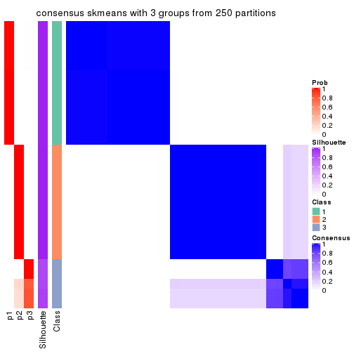
consensus_heatmap(res, k = 4)
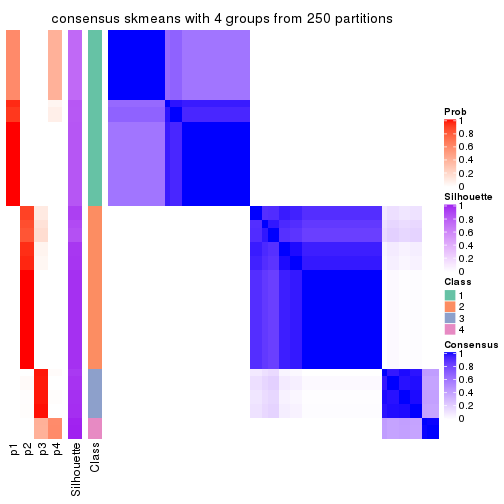
consensus_heatmap(res, k = 5)
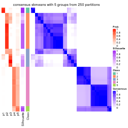
consensus_heatmap(res, k = 6)
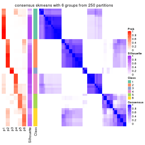
Heatmaps for the membership of samples in all partitions to see how consistent they are:
membership_heatmap(res, k = 2)

membership_heatmap(res, k = 3)
membership_heatmap(res, k = 4)
membership_heatmap(res, k = 5)
membership_heatmap(res, k = 6)
As soon as we have had the classes for columns, we can look for signatures which are significantly different between classes which can be candidate marks for certain classes. Following are the heatmaps for signatures.
Signature heatmaps where rows are scaled:
get_signatures(res, k = 2)

get_signatures(res, k = 3)
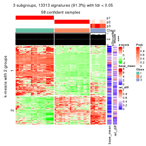
get_signatures(res, k = 4)
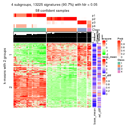
get_signatures(res, k = 5)
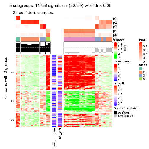
get_signatures(res, k = 6)
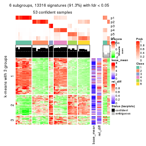
Signature heatmaps where rows are not scaled:
get_signatures(res, k = 2, scale_rows = FALSE)

get_signatures(res, k = 3, scale_rows = FALSE)
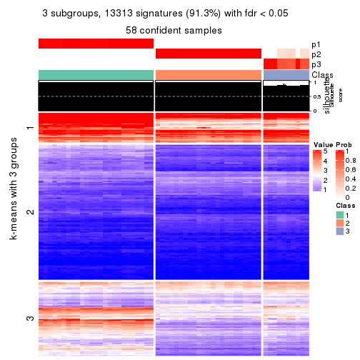
get_signatures(res, k = 4, scale_rows = FALSE)
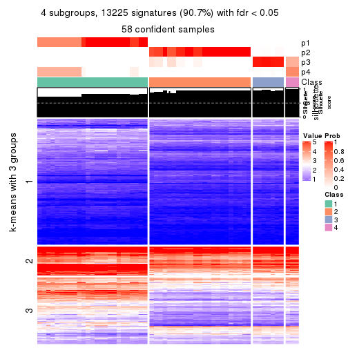
get_signatures(res, k = 5, scale_rows = FALSE)
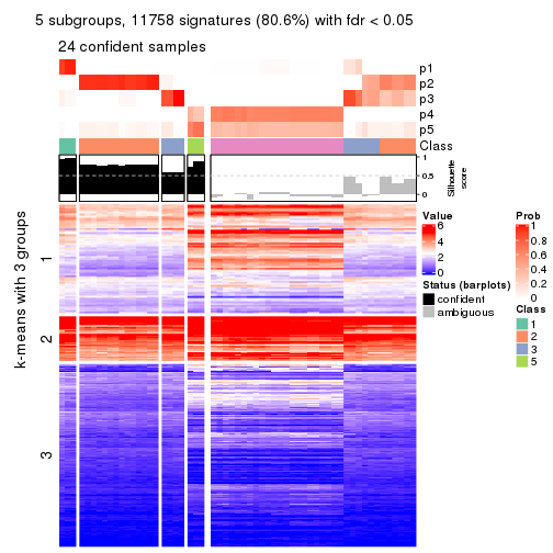
get_signatures(res, k = 6, scale_rows = FALSE)
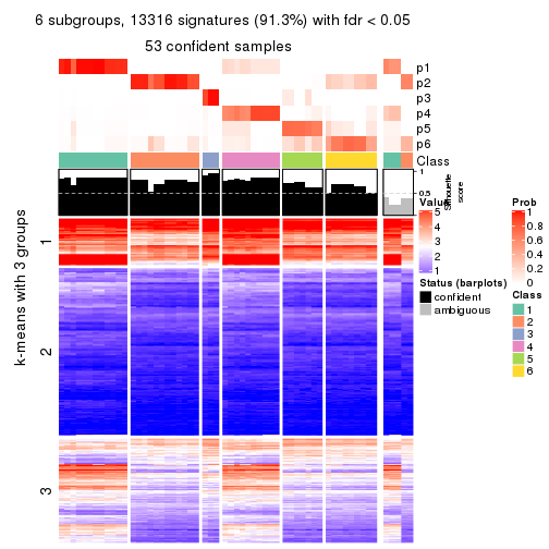
Compare the overlap of signatures from different k:
compare_signatures(res)
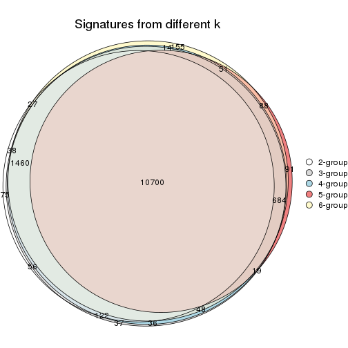
get_signature() returns a data frame invisibly. TO get the list of signatures, the function
call should be assigned to a variable explicitly. In following code, if plot argument is set
to FALSE, no heatmap is plotted while only the differential analysis is performed.
# code only for demonstration
tb = get_signature(res, k = ..., plot = FALSE)
An example of the output of tb is:
#>   which_row         fdr    mean_1    mean_2 scaled_mean_1 scaled_mean_2 km
#> 1        38 0.042760348  8.373488  9.131774    -0.5533452     0.5164555  1
#> 2        40 0.018707592  7.106213  8.469186    -0.6173731     0.5762149  1
#> 3        55 0.019134737 10.221463 11.207825    -0.6159697     0.5749050  1
#> 4        59 0.006059896  5.921854  7.869574    -0.6899429     0.6439467  1
#> 5        60 0.018055526  8.928898 10.211722    -0.6204761     0.5791110  1
#> 6        98 0.009384629 15.714769 14.887706     0.6635654    -0.6193277  2
...
The columns in tb are:
which_row: row indices corresponding to the input matrix.fdr: FDR for the differential test. mean_x: The mean value in group x.scaled_mean_x: The mean value in group x after rows are scaled.km: Row groups if k-means clustering is applied to rows.UMAP plot which shows how samples are separated.
dimension_reduction(res, k = 2, method = "UMAP")

dimension_reduction(res, k = 3, method = "UMAP")

dimension_reduction(res, k = 4, method = "UMAP")
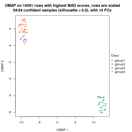
dimension_reduction(res, k = 5, method = "UMAP")
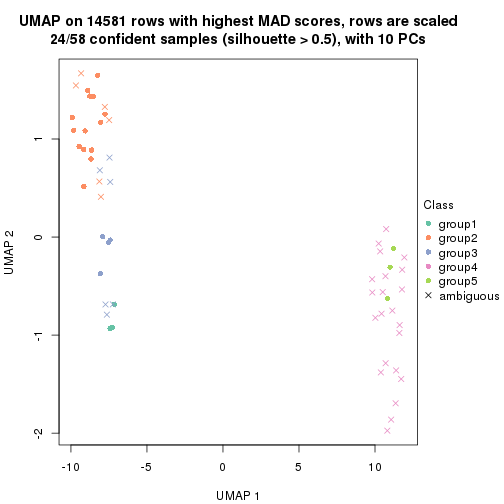
dimension_reduction(res, k = 6, method = "UMAP")
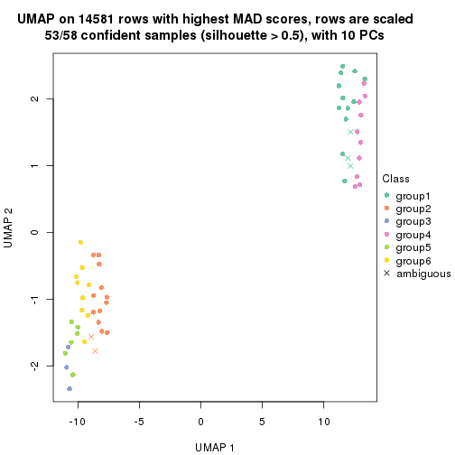
Following heatmap shows how subgroups are split when increasing k:
collect_classes(res)
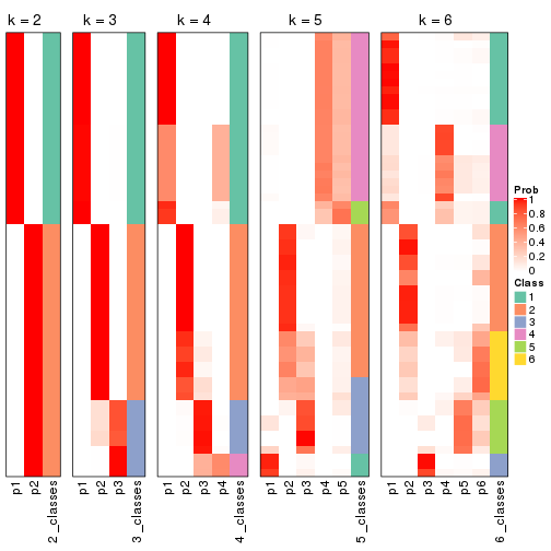
If matrix rows can be associated to genes, consider to use functional_enrichment(res,
...) to perform function enrichment for the signature genes. See this vignette for more detailed explanations.
The object with results only for a single top-value method and a single partition method can be extracted as:
res = res_list["MAD", "pam"]
# you can also extract it by
# res = res_list["MAD:pam"]
A summary of res and all the functions that can be applied to it:
res
#> A 'ConsensusPartition' object with k = 2, 3, 4, 5, 6.
#>   On a matrix with 14581 rows and 58 columns.
#>   Top rows (1000, 2000, 3000, 4000, 5000) are extracted by 'MAD' method.
#>   Subgroups are detected by 'pam' method.
#>   Performed in total 1250 partitions by row resampling.
#>   Best k for subgroups seems to be 2.
#>
#> Following methods can be applied to this 'ConsensusPartition' object:
#>  [1] "cola_report"             "collect_classes"         "collect_plots"
#>  [4] "collect_stats"           "colnames"                "compare_signatures"
#>  [7] "consensus_heatmap"       "dimension_reduction"     "functional_enrichment"
#> [10] "get_anno_col"            "get_anno"                "get_classes"
#> [13] "get_consensus"           "get_matrix"              "get_membership"
#> [16] "get_param"               "get_signatures"          "get_stats"
#> [19] "is_best_k"               "is_stable_k"             "membership_heatmap"
#> [22] "ncol"                    "nrow"                    "plot_ecdf"
#> [25] "rownames"                "select_partition_number" "show"
#> [28] "suggest_best_k"          "test_to_known_factors"
collect_plots() function collects all the plots made from res for all k (number of partitions)
into one single page to provide an easy and fast comparison between different k.
collect_plots(res)
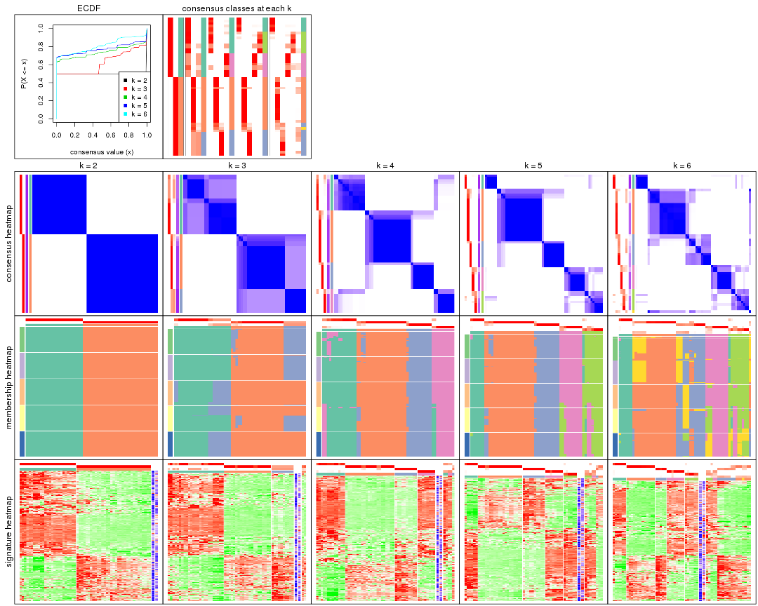
The plots are:
k and the heatmap of
predicted classes for each k.k.k.k.All the plots in panels can be made by individual functions and they are plotted later in this section.
select_partition_number() produces several plots showing different
statistics for choosing “optimized” k. There are following statistics:
k;k, the area increased is defined as \(A_k - A_{k-1}\).The detailed explanations of these statistics can be found in the cola vignette.
Generally speaking, lower PAC score, higher mean silhouette score or higher
concordance corresponds to better partition. Rand index and Jaccard index
measure how similar the current partition is compared to partition with k-1.
If they are too similar, we won't accept k is better than k-1.
select_partition_number(res)
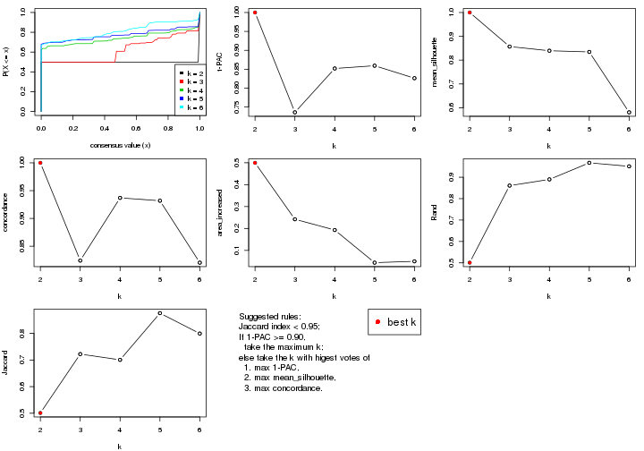
The numeric values for all these statistics can be obtained by get_stats().
get_stats(res)
#>   k 1-PAC mean_silhouette concordance area_increased  Rand Jaccard
#> 2 2 1.000           1.000       1.000         0.4996 0.501   0.501
#> 3 3 0.736           0.857       0.824         0.2420 0.861   0.722
#> 4 4 0.852           0.839       0.937         0.1929 0.890   0.701
#> 5 5 0.859           0.834       0.932         0.0440 0.967   0.876
#> 6 6 0.826           0.581       0.820         0.0501 0.951   0.800
suggest_best_k() suggests the best \(k\) based on these statistics. The rules are as follows:
suggest_best_k(res)
#> [1] 2
Following shows the table of the partitions (You need to click the show/hide
code output link to see it). The membership matrix (columns with name p*)
is inferred by
clue::cl_consensus()
function with the SE method. Basically the value in the membership matrix
represents the probability to belong to a certain group. The finall class
label for an item is determined with the group with highest probability it
belongs to.
In get_classes() function, the entropy is calculated from the membership
matrix and the silhouette score is calculated from the consensus matrix.
cbind(get_classes(res, k = 2), get_membership(res, k = 2))
#>           class entropy silhouette p1 p2
#> ERR789082     2       0          1  0  1
#> ERR789083     2       0          1  0  1
#> ERR789191     2       0          1  0  1
#> ERR789192     2       0          1  0  1
#> ERR789213     1       0          1  1  0
#> ERR789385     1       0          1  1  0
#> ERR789393     1       0          1  1  0
#> ERR789394     1       0          1  1  0
#> ERR789193     2       0          1  0  1
#> ERR789194     2       0          1  0  1
#> ERR789195     2       0          1  0  1
#> ERR789196     2       0          1  0  1
#> ERR789388     1       0          1  1  0
#> ERR789197     2       0          1  0  1
#> ERR789198     2       0          1  0  1
#> ERR789214     1       0          1  1  0
#> ERR789397     1       0          1  1  0
#> ERR789398     1       0          1  1  0
#> ERR789199     2       0          1  0  1
#> ERR789200     2       0          1  0  1
#> ERR789201     2       0          1  0  1
#> ERR789202     2       0          1  0  1
#> ERR789215     1       0          1  1  0
#> ERR789203     2       0          1  0  1
#> ERR789204     2       0          1  0  1
#> ERR789383     1       0          1  1  0
#> ERR789205     2       0          1  0  1
#> ERR789206     2       0          1  0  1
#> ERR789399     1       0          1  1  0
#> ERR789400     1       0          1  1  0
#> ERR789207     2       0          1  0  1
#> ERR789208     2       0          1  0  1
#> ERR789209     2       0          1  0  1
#> ERR789210     2       0          1  0  1
#> ERR789211     2       0          1  0  1
#> ERR789212     2       0          1  0  1
#> ERR789386     1       0          1  1  0
#> ERR789076     2       0          1  0  1
#> ERR789077     2       0          1  0  1
#> ERR789384     1       0          1  1  0
#> ERR789078     2       0          1  0  1
#> ERR789079     2       0          1  0  1
#> ERR789216     1       0          1  1  0
#> ERR789080     2       0          1  0  1
#> ERR789387     1       0          1  1  0
#> ERR789081     2       0          1  0  1
#> ERR789064     2       0          1  0  1
#> ERR779485     2       0          1  0  1
#> ERR789065     2       0          1  0  1
#> ERR789401     1       0          1  1  0
#> ERR789402     1       0          1  1  0
#> ERR789403     1       0          1  1  0
#> ERR789389     1       0          1  1  0
#> ERR789395     1       0          1  1  0
#> ERR789396     1       0          1  1  0
#> ERR789390     1       0          1  1  0
#> ERR789391     1       0          1  1  0
#> ERR789392     1       0          1  1  0
cbind(get_classes(res, k = 3), get_membership(res, k = 3))
#>           class entropy silhouette    p1    p2    p3
#> ERR789082     2  0.0000     0.9317 0.000 1.000 0.000
#> ERR789083     2  0.0000     0.9317 0.000 1.000 0.000
#> ERR789191     2  0.0000     0.9317 0.000 1.000 0.000
#> ERR789192     2  0.0000     0.9317 0.000 1.000 0.000
#> ERR789213     1  0.6291     0.7506 0.532 0.000 0.468
#> ERR789385     1  0.6291     0.7506 0.532 0.000 0.468
#> ERR789393     1  0.6291     0.7506 0.532 0.000 0.468
#> ERR789394     1  0.6291     0.7506 0.532 0.000 0.468
#> ERR789193     3  0.6295     1.0000 0.000 0.472 0.528
#> ERR789194     3  0.6295     1.0000 0.000 0.472 0.528
#> ERR789195     3  0.6295     1.0000 0.000 0.472 0.528
#> ERR789196     3  0.6295     1.0000 0.000 0.472 0.528
#> ERR789388     1  0.0000     0.8412 1.000 0.000 0.000
#> ERR789197     2  0.2625     0.7945 0.000 0.916 0.084
#> ERR789198     2  0.2625     0.7945 0.000 0.916 0.084
#> ERR789214     1  0.6291     0.7506 0.532 0.000 0.468
#> ERR789397     1  0.4235     0.8115 0.824 0.000 0.176
#> ERR789398     1  0.4235     0.8115 0.824 0.000 0.176
#> ERR789199     2  0.0000     0.9317 0.000 1.000 0.000
#> ERR789200     2  0.0000     0.9317 0.000 1.000 0.000
#> ERR789201     2  0.4399     0.4845 0.000 0.812 0.188
#> ERR789202     2  0.3816     0.6254 0.000 0.852 0.148
#> ERR789215     1  0.0000     0.8412 1.000 0.000 0.000
#> ERR789203     3  0.6295     1.0000 0.000 0.472 0.528
#> ERR789204     3  0.6295     1.0000 0.000 0.472 0.528
#> ERR789383     1  0.0237     0.8406 0.996 0.000 0.004
#> ERR789205     3  0.6295     1.0000 0.000 0.472 0.528
#> ERR789206     3  0.6295     1.0000 0.000 0.472 0.528
#> ERR789399     1  0.0000     0.8412 1.000 0.000 0.000
#> ERR789400     1  0.0000     0.8412 1.000 0.000 0.000
#> ERR789207     2  0.0000     0.9317 0.000 1.000 0.000
#> ERR789208     2  0.0000     0.9317 0.000 1.000 0.000
#> ERR789209     2  0.0000     0.9317 0.000 1.000 0.000
#> ERR789210     2  0.0000     0.9317 0.000 1.000 0.000
#> ERR789211     2  0.0000     0.9317 0.000 1.000 0.000
#> ERR789212     2  0.0000     0.9317 0.000 1.000 0.000
#> ERR789386     1  0.5497     0.7869 0.708 0.000 0.292
#> ERR789076     2  0.5254     0.0995 0.000 0.736 0.264
#> ERR789077     2  0.0000     0.9317 0.000 1.000 0.000
#> ERR789384     1  0.6291     0.7506 0.532 0.000 0.468
#> ERR789078     2  0.0000     0.9317 0.000 1.000 0.000
#> ERR789079     2  0.0000     0.9317 0.000 1.000 0.000
#> ERR789216     1  0.6291     0.7506 0.532 0.000 0.468
#> ERR789080     2  0.0000     0.9317 0.000 1.000 0.000
#> ERR789387     1  0.5497     0.7869 0.708 0.000 0.292
#> ERR789081     2  0.0000     0.9317 0.000 1.000 0.000
#> ERR789064     2  0.0000     0.9317 0.000 1.000 0.000
#> ERR779485     3  0.6295     1.0000 0.000 0.472 0.528
#> ERR789065     3  0.6295     1.0000 0.000 0.472 0.528
#> ERR789401     1  0.0237     0.8406 0.996 0.000 0.004
#> ERR789402     1  0.0237     0.8406 0.996 0.000 0.004
#> ERR789403     1  0.0237     0.8406 0.996 0.000 0.004
#> ERR789389     1  0.0237     0.8406 0.996 0.000 0.004
#> ERR789395     1  0.0237     0.8406 0.996 0.000 0.004
#> ERR789396     1  0.0237     0.8406 0.996 0.000 0.004
#> ERR789390     1  0.0000     0.8412 1.000 0.000 0.000
#> ERR789391     1  0.0000     0.8412 1.000 0.000 0.000
#> ERR789392     1  0.6291     0.7506 0.532 0.000 0.468
cbind(get_classes(res, k = 4), get_membership(res, k = 4))
#>           class entropy silhouette    p1    p2    p3    p4
#> ERR789082     2  0.0000      0.949 0.000 1.000 0.000 0.000
#> ERR789083     2  0.0000      0.949 0.000 1.000 0.000 0.000
#> ERR789191     2  0.0000      0.949 0.000 1.000 0.000 0.000
#> ERR789192     2  0.0000      0.949 0.000 1.000 0.000 0.000
#> ERR789213     4  0.0000      0.884 0.000 0.000 0.000 1.000
#> ERR789385     4  0.0000      0.884 0.000 0.000 0.000 1.000
#> ERR789393     4  0.0000      0.884 0.000 0.000 0.000 1.000
#> ERR789394     4  0.0000      0.884 0.000 0.000 0.000 1.000
#> ERR789193     3  0.0000      0.958 0.000 0.000 1.000 0.000
#> ERR789194     3  0.0000      0.958 0.000 0.000 1.000 0.000
#> ERR789195     3  0.0000      0.958 0.000 0.000 1.000 0.000
#> ERR789196     3  0.0000      0.958 0.000 0.000 1.000 0.000
#> ERR789388     1  0.3726      0.691 0.788 0.000 0.000 0.212
#> ERR789197     2  0.4564      0.509 0.000 0.672 0.328 0.000
#> ERR789198     2  0.4564      0.509 0.000 0.672 0.328 0.000
#> ERR789214     4  0.0000      0.884 0.000 0.000 0.000 1.000
#> ERR789397     4  0.4898      0.249 0.416 0.000 0.000 0.584
#> ERR789398     4  0.4898      0.249 0.416 0.000 0.000 0.584
#> ERR789199     2  0.0000      0.949 0.000 1.000 0.000 0.000
#> ERR789200     2  0.0000      0.949 0.000 1.000 0.000 0.000
#> ERR789201     2  0.3486      0.760 0.000 0.812 0.188 0.000
#> ERR789202     2  0.3024      0.810 0.000 0.852 0.148 0.000
#> ERR789215     1  0.0336      0.874 0.992 0.000 0.000 0.008
#> ERR789203     3  0.0000      0.958 0.000 0.000 1.000 0.000
#> ERR789204     3  0.0000      0.958 0.000 0.000 1.000 0.000
#> ERR789383     1  0.0000      0.872 1.000 0.000 0.000 0.000
#> ERR789205     3  0.0000      0.958 0.000 0.000 1.000 0.000
#> ERR789206     3  0.0000      0.958 0.000 0.000 1.000 0.000
#> ERR789399     1  0.0336      0.874 0.992 0.000 0.000 0.008
#> ERR789400     1  0.0336      0.874 0.992 0.000 0.000 0.008
#> ERR789207     2  0.0000      0.949 0.000 1.000 0.000 0.000
#> ERR789208     2  0.0000      0.949 0.000 1.000 0.000 0.000
#> ERR789209     2  0.0000      0.949 0.000 1.000 0.000 0.000
#> ERR789210     2  0.0000      0.949 0.000 1.000 0.000 0.000
#> ERR789211     2  0.0000      0.949 0.000 1.000 0.000 0.000
#> ERR789212     2  0.0000      0.949 0.000 1.000 0.000 0.000
#> ERR789386     1  0.4967      0.207 0.548 0.000 0.000 0.452
#> ERR789076     3  0.4585      0.458 0.000 0.332 0.668 0.000
#> ERR789077     2  0.0000      0.949 0.000 1.000 0.000 0.000
#> ERR789384     4  0.0000      0.884 0.000 0.000 0.000 1.000
#> ERR789078     2  0.0000      0.949 0.000 1.000 0.000 0.000
#> ERR789079     2  0.0000      0.949 0.000 1.000 0.000 0.000
#> ERR789216     4  0.0000      0.884 0.000 0.000 0.000 1.000
#> ERR789080     2  0.0000      0.949 0.000 1.000 0.000 0.000
#> ERR789387     1  0.4967      0.207 0.548 0.000 0.000 0.452
#> ERR789081     2  0.0000      0.949 0.000 1.000 0.000 0.000
#> ERR789064     2  0.0000      0.949 0.000 1.000 0.000 0.000
#> ERR779485     3  0.0000      0.958 0.000 0.000 1.000 0.000
#> ERR789065     3  0.0000      0.958 0.000 0.000 1.000 0.000
#> ERR789401     1  0.0000      0.872 1.000 0.000 0.000 0.000
#> ERR789402     1  0.1474      0.858 0.948 0.000 0.000 0.052
#> ERR789403     1  0.0000      0.872 1.000 0.000 0.000 0.000
#> ERR789389     1  0.3266      0.747 0.832 0.000 0.000 0.168
#> ERR789395     1  0.1211      0.864 0.960 0.000 0.000 0.040
#> ERR789396     1  0.1118      0.866 0.964 0.000 0.000 0.036
#> ERR789390     1  0.1022      0.867 0.968 0.000 0.000 0.032
#> ERR789391     1  0.1022      0.867 0.968 0.000 0.000 0.032
#> ERR789392     4  0.0000      0.884 0.000 0.000 0.000 1.000
cbind(get_classes(res, k = 5), get_membership(res, k = 5))
#>           class entropy silhouette    p1    p2    p3    p4    p5
#> ERR789082     2  0.0000      0.947 0.000 1.000 0.000 0.000 0.000
#> ERR789083     2  0.0000      0.947 0.000 1.000 0.000 0.000 0.000
#> ERR789191     2  0.0000      0.947 0.000 1.000 0.000 0.000 0.000
#> ERR789192     2  0.0000      0.947 0.000 1.000 0.000 0.000 0.000
#> ERR789213     4  0.0000      0.856 0.000 0.000 0.000 1.000 0.000
#> ERR789385     4  0.0000      0.856 0.000 0.000 0.000 1.000 0.000
#> ERR789393     4  0.0000      0.856 0.000 0.000 0.000 1.000 0.000
#> ERR789394     4  0.0000      0.856 0.000 0.000 0.000 1.000 0.000
#> ERR789193     3  0.0000      0.955 0.000 0.000 1.000 0.000 0.000
#> ERR789194     3  0.0000      0.955 0.000 0.000 1.000 0.000 0.000
#> ERR789195     3  0.0000      0.955 0.000 0.000 1.000 0.000 0.000
#> ERR789196     3  0.0000      0.955 0.000 0.000 1.000 0.000 0.000
#> ERR789388     5  0.4339      0.362 0.336 0.000 0.000 0.012 0.652
#> ERR789197     2  0.3949      0.500 0.000 0.668 0.332 0.000 0.000
#> ERR789198     2  0.3949      0.500 0.000 0.668 0.332 0.000 0.000
#> ERR789214     4  0.2648      0.739 0.000 0.000 0.000 0.848 0.152
#> ERR789397     4  0.4262      0.327 0.000 0.000 0.000 0.560 0.440
#> ERR789398     4  0.4262      0.327 0.000 0.000 0.000 0.560 0.440
#> ERR789199     2  0.0000      0.947 0.000 1.000 0.000 0.000 0.000
#> ERR789200     2  0.0000      0.947 0.000 1.000 0.000 0.000 0.000
#> ERR789201     2  0.3003      0.760 0.000 0.812 0.188 0.000 0.000
#> ERR789202     2  0.2605      0.809 0.000 0.852 0.148 0.000 0.000
#> ERR789215     5  0.2424      0.718 0.000 0.000 0.000 0.132 0.868
#> ERR789203     3  0.0000      0.955 0.000 0.000 1.000 0.000 0.000
#> ERR789204     3  0.0000      0.955 0.000 0.000 1.000 0.000 0.000
#> ERR789383     5  0.2648      0.694 0.152 0.000 0.000 0.000 0.848
#> ERR789205     3  0.0000      0.955 0.000 0.000 1.000 0.000 0.000
#> ERR789206     3  0.0000      0.955 0.000 0.000 1.000 0.000 0.000
#> ERR789399     5  0.0000      0.772 0.000 0.000 0.000 0.000 1.000
#> ERR789400     5  0.0000      0.772 0.000 0.000 0.000 0.000 1.000
#> ERR789207     2  0.0000      0.947 0.000 1.000 0.000 0.000 0.000
#> ERR789208     2  0.0000      0.947 0.000 1.000 0.000 0.000 0.000
#> ERR789209     2  0.0000      0.947 0.000 1.000 0.000 0.000 0.000
#> ERR789210     2  0.0000      0.947 0.000 1.000 0.000 0.000 0.000
#> ERR789211     2  0.0000      0.947 0.000 1.000 0.000 0.000 0.000
#> ERR789212     2  0.0000      0.947 0.000 1.000 0.000 0.000 0.000
#> ERR789386     5  0.4262      0.340 0.000 0.000 0.000 0.440 0.560
#> ERR789076     3  0.3932      0.468 0.000 0.328 0.672 0.000 0.000
#> ERR789077     2  0.0000      0.947 0.000 1.000 0.000 0.000 0.000
#> ERR789384     4  0.0000      0.856 0.000 0.000 0.000 1.000 0.000
#> ERR789078     2  0.0000      0.947 0.000 1.000 0.000 0.000 0.000
#> ERR789079     2  0.0000      0.947 0.000 1.000 0.000 0.000 0.000
#> ERR789216     4  0.0000      0.856 0.000 0.000 0.000 1.000 0.000
#> ERR789080     2  0.0000      0.947 0.000 1.000 0.000 0.000 0.000
#> ERR789387     5  0.4268      0.332 0.000 0.000 0.000 0.444 0.556
#> ERR789081     2  0.0000      0.947 0.000 1.000 0.000 0.000 0.000
#> ERR789064     2  0.0000      0.947 0.000 1.000 0.000 0.000 0.000
#> ERR779485     3  0.0000      0.955 0.000 0.000 1.000 0.000 0.000
#> ERR789065     3  0.0000      0.955 0.000 0.000 1.000 0.000 0.000
#> ERR789401     1  0.0000      0.985 1.000 0.000 0.000 0.000 0.000
#> ERR789402     1  0.0000      0.985 1.000 0.000 0.000 0.000 0.000
#> ERR789403     1  0.0000      0.985 1.000 0.000 0.000 0.000 0.000
#> ERR789389     1  0.1907      0.920 0.928 0.000 0.000 0.044 0.028
#> ERR789395     1  0.0000      0.985 1.000 0.000 0.000 0.000 0.000
#> ERR789396     1  0.0000      0.985 1.000 0.000 0.000 0.000 0.000
#> ERR789390     5  0.0162      0.771 0.000 0.000 0.000 0.004 0.996
#> ERR789391     5  0.0000      0.772 0.000 0.000 0.000 0.000 1.000
#> ERR789392     4  0.0000      0.856 0.000 0.000 0.000 1.000 0.000
cbind(get_classes(res, k = 6), get_membership(res, k = 6))
#>           class entropy silhouette    p1    p2    p3    p4    p5    p6
#> ERR789082     2  0.3563     0.1890 0.000 0.664 0.000 0.000 0.000 0.336
#> ERR789083     2  0.3563     0.1890 0.000 0.664 0.000 0.000 0.000 0.336
#> ERR789191     2  0.0363     0.7767 0.000 0.988 0.000 0.000 0.000 0.012
#> ERR789192     2  0.0363     0.7767 0.000 0.988 0.000 0.000 0.000 0.012
#> ERR789213     4  0.0000     0.8333 0.000 0.000 0.000 1.000 0.000 0.000
#> ERR789385     4  0.0000     0.8333 0.000 0.000 0.000 1.000 0.000 0.000
#> ERR789393     4  0.0000     0.8333 0.000 0.000 0.000 1.000 0.000 0.000
#> ERR789394     4  0.0000     0.8333 0.000 0.000 0.000 1.000 0.000 0.000
#> ERR789193     3  0.3864     0.4383 0.000 0.000 0.520 0.000 0.000 0.480
#> ERR789194     3  0.3864     0.4383 0.000 0.000 0.520 0.000 0.000 0.480
#> ERR789195     3  0.3717     0.2445 0.000 0.000 0.616 0.000 0.000 0.384
#> ERR789196     3  0.3717     0.2445 0.000 0.000 0.616 0.000 0.000 0.384
#> ERR789388     5  0.6039     0.2703 0.324 0.000 0.000 0.012 0.480 0.184
#> ERR789197     6  0.6005     0.0000 0.000 0.380 0.236 0.000 0.000 0.384
#> ERR789198     2  0.5983    -0.9815 0.000 0.388 0.228 0.000 0.000 0.384
#> ERR789214     4  0.4680     0.5960 0.000 0.000 0.000 0.684 0.132 0.184
#> ERR789397     4  0.5593     0.3968 0.000 0.000 0.000 0.536 0.280 0.184
#> ERR789398     4  0.5593     0.3968 0.000 0.000 0.000 0.536 0.280 0.184
#> ERR789199     2  0.3531     0.1996 0.000 0.672 0.000 0.000 0.000 0.328
#> ERR789200     2  0.3531     0.1996 0.000 0.672 0.000 0.000 0.000 0.328
#> ERR789201     3  0.4109     0.1229 0.000 0.412 0.576 0.000 0.000 0.012
#> ERR789202     3  0.4165     0.0589 0.000 0.452 0.536 0.000 0.000 0.012
#> ERR789215     5  0.1957     0.7058 0.000 0.000 0.000 0.112 0.888 0.000
#> ERR789203     3  0.0000     0.6201 0.000 0.000 1.000 0.000 0.000 0.000
#> ERR789204     3  0.0000     0.6201 0.000 0.000 1.000 0.000 0.000 0.000
#> ERR789383     5  0.2178     0.6735 0.132 0.000 0.000 0.000 0.868 0.000
#> ERR789205     3  0.0000     0.6201 0.000 0.000 1.000 0.000 0.000 0.000
#> ERR789206     3  0.0000     0.6201 0.000 0.000 1.000 0.000 0.000 0.000
#> ERR789399     5  0.0000     0.7412 0.000 0.000 0.000 0.000 1.000 0.000
#> ERR789400     5  0.0000     0.7412 0.000 0.000 0.000 0.000 1.000 0.000
#> ERR789207     2  0.0000     0.7798 0.000 1.000 0.000 0.000 0.000 0.000
#> ERR789208     2  0.0000     0.7798 0.000 1.000 0.000 0.000 0.000 0.000
#> ERR789209     2  0.0000     0.7798 0.000 1.000 0.000 0.000 0.000 0.000
#> ERR789210     2  0.0000     0.7798 0.000 1.000 0.000 0.000 0.000 0.000
#> ERR789211     2  0.0000     0.7798 0.000 1.000 0.000 0.000 0.000 0.000
#> ERR789212     2  0.0000     0.7798 0.000 1.000 0.000 0.000 0.000 0.000
#> ERR789386     5  0.3833     0.3720 0.000 0.000 0.000 0.444 0.556 0.000
#> ERR789076     3  0.4658     0.0996 0.000 0.048 0.568 0.000 0.000 0.384
#> ERR789077     2  0.0260     0.7785 0.000 0.992 0.000 0.000 0.000 0.008
#> ERR789384     4  0.0000     0.8333 0.000 0.000 0.000 1.000 0.000 0.000
#> ERR789078     2  0.0260     0.7785 0.000 0.992 0.000 0.000 0.000 0.008
#> ERR789079     2  0.0146     0.7797 0.000 0.996 0.000 0.000 0.000 0.004
#> ERR789216     4  0.0146     0.8317 0.000 0.000 0.000 0.996 0.000 0.004
#> ERR789080     2  0.0146     0.7797 0.000 0.996 0.000 0.000 0.000 0.004
#> ERR789387     5  0.3838     0.3648 0.000 0.000 0.000 0.448 0.552 0.000
#> ERR789081     2  0.0146     0.7797 0.000 0.996 0.000 0.000 0.000 0.004
#> ERR789064     2  0.3499     0.2288 0.000 0.680 0.000 0.000 0.000 0.320
#> ERR779485     3  0.3817     0.4489 0.000 0.000 0.568 0.000 0.000 0.432
#> ERR789065     3  0.0865     0.6093 0.000 0.000 0.964 0.000 0.000 0.036
#> ERR789401     1  0.0000     0.9846 1.000 0.000 0.000 0.000 0.000 0.000
#> ERR789402     1  0.0000     0.9846 1.000 0.000 0.000 0.000 0.000 0.000
#> ERR789403     1  0.0000     0.9846 1.000 0.000 0.000 0.000 0.000 0.000
#> ERR789389     1  0.1789     0.9194 0.924 0.000 0.000 0.044 0.032 0.000
#> ERR789395     1  0.0000     0.9846 1.000 0.000 0.000 0.000 0.000 0.000
#> ERR789396     1  0.0000     0.9846 1.000 0.000 0.000 0.000 0.000 0.000
#> ERR789390     5  0.2219     0.7132 0.000 0.000 0.000 0.000 0.864 0.136
#> ERR789391     5  0.2491     0.7008 0.000 0.000 0.000 0.000 0.836 0.164
#> ERR789392     4  0.0000     0.8333 0.000 0.000 0.000 1.000 0.000 0.000
Heatmaps for the consensus matrix. It visualizes the probability of two samples to be in a same group.
consensus_heatmap(res, k = 2)

consensus_heatmap(res, k = 3)
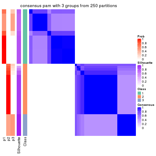
consensus_heatmap(res, k = 4)
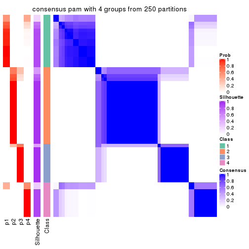
consensus_heatmap(res, k = 5)
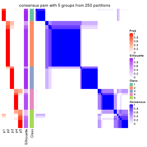
consensus_heatmap(res, k = 6)

Heatmaps for the membership of samples in all partitions to see how consistent they are:
membership_heatmap(res, k = 2)
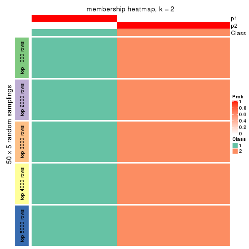
membership_heatmap(res, k = 3)
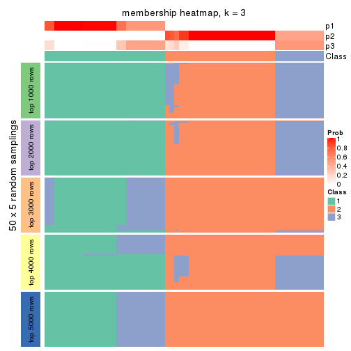
membership_heatmap(res, k = 4)
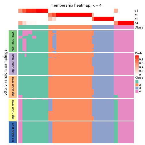
membership_heatmap(res, k = 5)
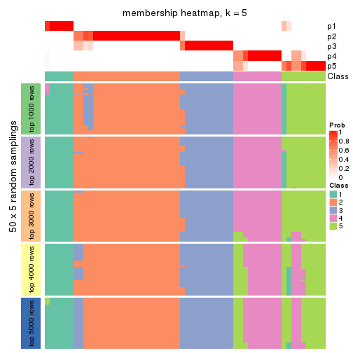
membership_heatmap(res, k = 6)
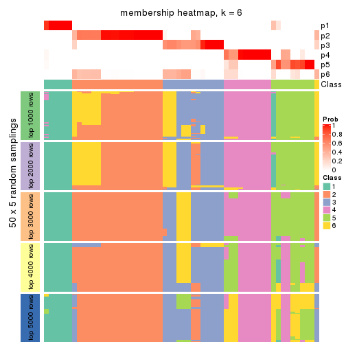
As soon as we have had the classes for columns, we can look for signatures which are significantly different between classes which can be candidate marks for certain classes. Following are the heatmaps for signatures.
Signature heatmaps where rows are scaled:
get_signatures(res, k = 2)

get_signatures(res, k = 3)
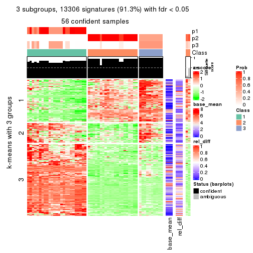
get_signatures(res, k = 4)
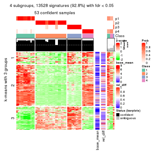
get_signatures(res, k = 5)
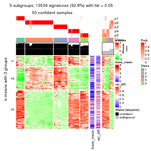
get_signatures(res, k = 6)
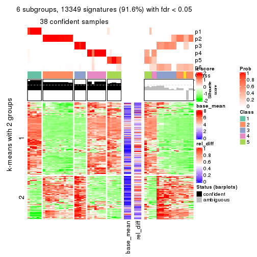
Signature heatmaps where rows are not scaled:
get_signatures(res, k = 2, scale_rows = FALSE)

get_signatures(res, k = 3, scale_rows = FALSE)
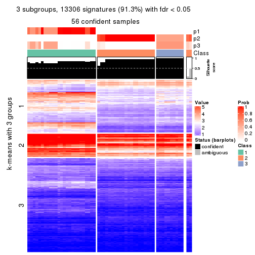
get_signatures(res, k = 4, scale_rows = FALSE)
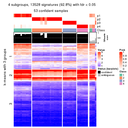
get_signatures(res, k = 5, scale_rows = FALSE)
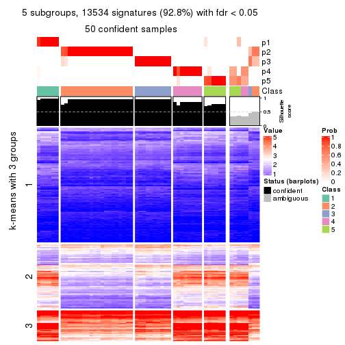
get_signatures(res, k = 6, scale_rows = FALSE)
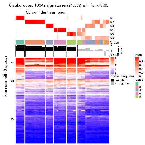
Compare the overlap of signatures from different k:
compare_signatures(res)
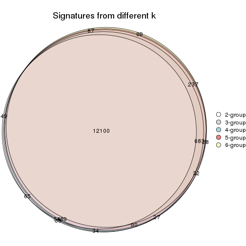
get_signature() returns a data frame invisibly. TO get the list of signatures, the function
call should be assigned to a variable explicitly. In following code, if plot argument is set
to FALSE, no heatmap is plotted while only the differential analysis is performed.
# code only for demonstration
tb = get_signature(res, k = ..., plot = FALSE)
An example of the output of tb is:
#>   which_row         fdr    mean_1    mean_2 scaled_mean_1 scaled_mean_2 km
#> 1        38 0.042760348  8.373488  9.131774    -0.5533452     0.5164555  1
#> 2        40 0.018707592  7.106213  8.469186    -0.6173731     0.5762149  1
#> 3        55 0.019134737 10.221463 11.207825    -0.6159697     0.5749050  1
#> 4        59 0.006059896  5.921854  7.869574    -0.6899429     0.6439467  1
#> 5        60 0.018055526  8.928898 10.211722    -0.6204761     0.5791110  1
#> 6        98 0.009384629 15.714769 14.887706     0.6635654    -0.6193277  2
...
The columns in tb are:
which_row: row indices corresponding to the input matrix.fdr: FDR for the differential test. mean_x: The mean value in group x.scaled_mean_x: The mean value in group x after rows are scaled.km: Row groups if k-means clustering is applied to rows.UMAP plot which shows how samples are separated.
dimension_reduction(res, k = 2, method = "UMAP")
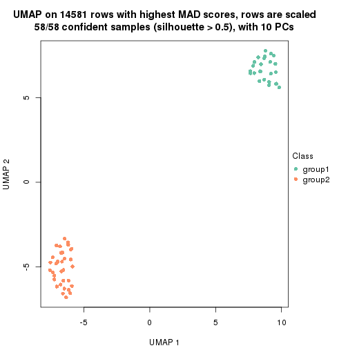
dimension_reduction(res, k = 3, method = "UMAP")
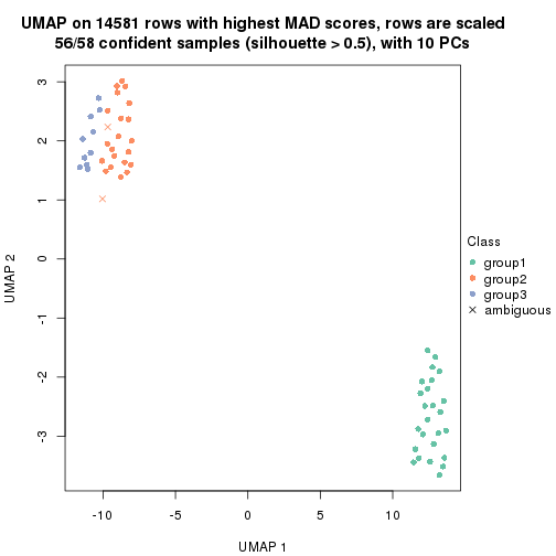
dimension_reduction(res, k = 4, method = "UMAP")
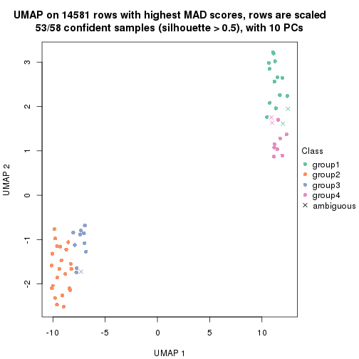
dimension_reduction(res, k = 5, method = "UMAP")
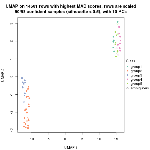
dimension_reduction(res, k = 6, method = "UMAP")
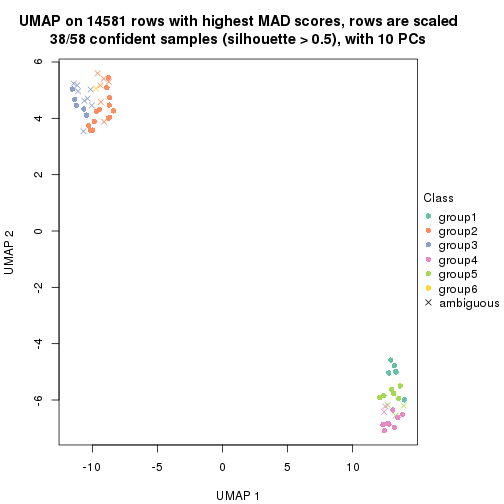
Following heatmap shows how subgroups are split when increasing k:
collect_classes(res)
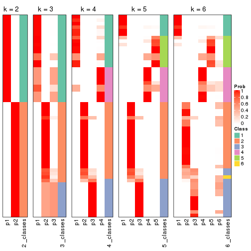
If matrix rows can be associated to genes, consider to use functional_enrichment(res,
...) to perform function enrichment for the signature genes. See this vignette for more detailed explanations.
The object with results only for a single top-value method and a single partition method can be extracted as:
res = res_list["MAD", "mclust"]
# you can also extract it by
# res = res_list["MAD:mclust"]
A summary of res and all the functions that can be applied to it:
res
#> A 'ConsensusPartition' object with k = 2, 3, 4, 5, 6.
#>   On a matrix with 14581 rows and 58 columns.
#>   Top rows (1000, 2000, 3000, 4000, 5000) are extracted by 'MAD' method.
#>   Subgroups are detected by 'mclust' method.
#>   Performed in total 1250 partitions by row resampling.
#>   Best k for subgroups seems to be 2.
#>
#> Following methods can be applied to this 'ConsensusPartition' object:
#>  [1] "cola_report"             "collect_classes"         "collect_plots"
#>  [4] "collect_stats"           "colnames"                "compare_signatures"
#>  [7] "consensus_heatmap"       "dimension_reduction"     "functional_enrichment"
#> [10] "get_anno_col"            "get_anno"                "get_classes"
#> [13] "get_consensus"           "get_matrix"              "get_membership"
#> [16] "get_param"               "get_signatures"          "get_stats"
#> [19] "is_best_k"               "is_stable_k"             "membership_heatmap"
#> [22] "ncol"                    "nrow"                    "plot_ecdf"
#> [25] "rownames"                "select_partition_number" "show"
#> [28] "suggest_best_k"          "test_to_known_factors"
collect_plots() function collects all the plots made from res for all k (number of partitions)
into one single page to provide an easy and fast comparison between different k.
collect_plots(res)
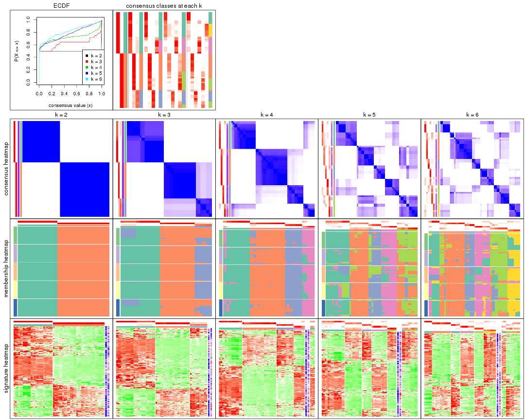
The plots are:
k and the heatmap of
predicted classes for each k.k.k.k.All the plots in panels can be made by individual functions and they are plotted later in this section.
select_partition_number() produces several plots showing different
statistics for choosing “optimized” k. There are following statistics:
k;k, the area increased is defined as \(A_k - A_{k-1}\).The detailed explanations of these statistics can be found in the cola vignette.
Generally speaking, lower PAC score, higher mean silhouette score or higher
concordance corresponds to better partition. Rand index and Jaccard index
measure how similar the current partition is compared to partition with k-1.
If they are too similar, we won't accept k is better than k-1.
select_partition_number(res)
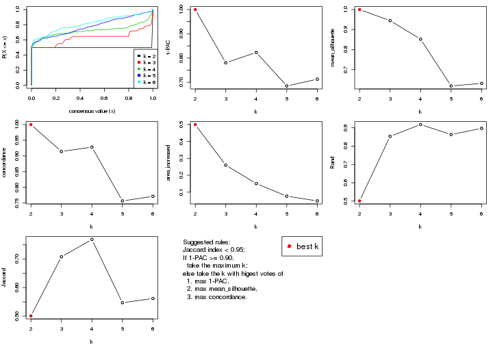
The numeric values for all these statistics can be obtained by get_stats().
get_stats(res)
#>   k 1-PAC mean_silhouette concordance area_increased  Rand Jaccard
#> 2 2 1.000           1.000       1.000         0.4996 0.501   0.501
#> 3 3 0.780           0.945       0.914         0.2594 0.854   0.708
#> 4 4 0.823           0.852       0.928         0.1504 0.918   0.768
#> 5 5 0.685           0.619       0.757         0.0762 0.863   0.547
#> 6 6 0.712           0.631       0.771         0.0481 0.897   0.562
suggest_best_k() suggests the best \(k\) based on these statistics. The rules are as follows:
suggest_best_k(res)
#> [1] 2
Following shows the table of the partitions (You need to click the show/hide
code output link to see it). The membership matrix (columns with name p*)
is inferred by
clue::cl_consensus()
function with the SE method. Basically the value in the membership matrix
represents the probability to belong to a certain group. The finall class
label for an item is determined with the group with highest probability it
belongs to.
In get_classes() function, the entropy is calculated from the membership
matrix and the silhouette score is calculated from the consensus matrix.
cbind(get_classes(res, k = 2), get_membership(res, k = 2))
#>           class entropy silhouette p1 p2
#> ERR789082     2       0          1  0  1
#> ERR789083     2       0          1  0  1
#> ERR789191     2       0          1  0  1
#> ERR789192     2       0          1  0  1
#> ERR789213     1       0          1  1  0
#> ERR789385     1       0          1  1  0
#> ERR789393     1       0          1  1  0
#> ERR789394     1       0          1  1  0
#> ERR789193     2       0          1  0  1
#> ERR789194     2       0          1  0  1
#> ERR789195     2       0          1  0  1
#> ERR789196     2       0          1  0  1
#> ERR789388     1       0          1  1  0
#> ERR789197     2       0          1  0  1
#> ERR789198     2       0          1  0  1
#> ERR789214     1       0          1  1  0
#> ERR789397     1       0          1  1  0
#> ERR789398     1       0          1  1  0
#> ERR789199     2       0          1  0  1
#> ERR789200     2       0          1  0  1
#> ERR789201     2       0          1  0  1
#> ERR789202     2       0          1  0  1
#> ERR789215     1       0          1  1  0
#> ERR789203     2       0          1  0  1
#> ERR789204     2       0          1  0  1
#> ERR789383     1       0          1  1  0
#> ERR789205     2       0          1  0  1
#> ERR789206     2       0          1  0  1
#> ERR789399     1       0          1  1  0
#> ERR789400     1       0          1  1  0
#> ERR789207     2       0          1  0  1
#> ERR789208     2       0          1  0  1
#> ERR789209     2       0          1  0  1
#> ERR789210     2       0          1  0  1
#> ERR789211     2       0          1  0  1
#> ERR789212     2       0          1  0  1
#> ERR789386     1       0          1  1  0
#> ERR789076     2       0          1  0  1
#> ERR789077     2       0          1  0  1
#> ERR789384     1       0          1  1  0
#> ERR789078     2       0          1  0  1
#> ERR789079     2       0          1  0  1
#> ERR789216     1       0          1  1  0
#> ERR789080     2       0          1  0  1
#> ERR789387     1       0          1  1  0
#> ERR789081     2       0          1  0  1
#> ERR789064     2       0          1  0  1
#> ERR779485     2       0          1  0  1
#> ERR789065     2       0          1  0  1
#> ERR789401     1       0          1  1  0
#> ERR789402     1       0          1  1  0
#> ERR789403     1       0          1  1  0
#> ERR789389     1       0          1  1  0
#> ERR789395     1       0          1  1  0
#> ERR789396     1       0          1  1  0
#> ERR789390     1       0          1  1  0
#> ERR789391     1       0          1  1  0
#> ERR789392     1       0          1  1  0
cbind(get_classes(res, k = 3), get_membership(res, k = 3))
#>           class entropy silhouette    p1    p2    p3
#> ERR789082     2  0.0237      0.992 0.000 0.996 0.004
#> ERR789083     2  0.0000      0.994 0.000 1.000 0.000
#> ERR789191     2  0.0000      0.994 0.000 1.000 0.000
#> ERR789192     2  0.0000      0.994 0.000 1.000 0.000
#> ERR789213     1  0.4555      0.896 0.800 0.000 0.200
#> ERR789385     1  0.4555      0.896 0.800 0.000 0.200
#> ERR789393     1  0.4555      0.896 0.800 0.000 0.200
#> ERR789394     1  0.4555      0.896 0.800 0.000 0.200
#> ERR789193     3  0.4504      0.919 0.000 0.196 0.804
#> ERR789194     3  0.4504      0.919 0.000 0.196 0.804
#> ERR789195     3  0.5216      0.933 0.000 0.260 0.740
#> ERR789196     3  0.5216      0.933 0.000 0.260 0.740
#> ERR789388     1  0.4399      0.900 0.812 0.000 0.188
#> ERR789197     2  0.0000      0.994 0.000 1.000 0.000
#> ERR789198     2  0.0000      0.994 0.000 1.000 0.000
#> ERR789214     1  0.4504      0.898 0.804 0.000 0.196
#> ERR789397     1  0.4504      0.898 0.804 0.000 0.196
#> ERR789398     1  0.4504      0.898 0.804 0.000 0.196
#> ERR789199     2  0.0424      0.989 0.000 0.992 0.008
#> ERR789200     2  0.0424      0.989 0.000 0.992 0.008
#> ERR789201     2  0.0747      0.981 0.000 0.984 0.016
#> ERR789202     2  0.0747      0.981 0.000 0.984 0.016
#> ERR789215     1  0.0000      0.930 1.000 0.000 0.000
#> ERR789203     3  0.5706      0.894 0.000 0.320 0.680
#> ERR789204     3  0.5706      0.894 0.000 0.320 0.680
#> ERR789383     1  0.0000      0.930 1.000 0.000 0.000
#> ERR789205     3  0.5254      0.934 0.000 0.264 0.736
#> ERR789206     3  0.5254      0.934 0.000 0.264 0.736
#> ERR789399     1  0.0000      0.930 1.000 0.000 0.000
#> ERR789400     1  0.0000      0.930 1.000 0.000 0.000
#> ERR789207     2  0.0000      0.994 0.000 1.000 0.000
#> ERR789208     2  0.0000      0.994 0.000 1.000 0.000
#> ERR789209     2  0.1163      0.965 0.000 0.972 0.028
#> ERR789210     2  0.0747      0.981 0.000 0.984 0.016
#> ERR789211     2  0.0000      0.994 0.000 1.000 0.000
#> ERR789212     2  0.0000      0.994 0.000 1.000 0.000
#> ERR789386     1  0.0000      0.930 1.000 0.000 0.000
#> ERR789076     3  0.5785      0.879 0.000 0.332 0.668
#> ERR789077     2  0.0000      0.994 0.000 1.000 0.000
#> ERR789384     1  0.3267      0.912 0.884 0.000 0.116
#> ERR789078     2  0.0000      0.994 0.000 1.000 0.000
#> ERR789079     2  0.0000      0.994 0.000 1.000 0.000
#> ERR789216     1  0.0000      0.930 1.000 0.000 0.000
#> ERR789080     2  0.0000      0.994 0.000 1.000 0.000
#> ERR789387     1  0.0000      0.930 1.000 0.000 0.000
#> ERR789081     2  0.0000      0.994 0.000 1.000 0.000
#> ERR789064     2  0.0000      0.994 0.000 1.000 0.000
#> ERR779485     3  0.4555      0.921 0.000 0.200 0.800
#> ERR789065     3  0.4750      0.929 0.000 0.216 0.784
#> ERR789401     1  0.0000      0.930 1.000 0.000 0.000
#> ERR789402     1  0.0000      0.930 1.000 0.000 0.000
#> ERR789403     1  0.0000      0.930 1.000 0.000 0.000
#> ERR789389     1  0.0000      0.930 1.000 0.000 0.000
#> ERR789395     1  0.0000      0.930 1.000 0.000 0.000
#> ERR789396     1  0.0000      0.930 1.000 0.000 0.000
#> ERR789390     1  0.2448      0.921 0.924 0.000 0.076
#> ERR789391     1  0.2448      0.921 0.924 0.000 0.076
#> ERR789392     1  0.4555      0.896 0.800 0.000 0.200
cbind(get_classes(res, k = 4), get_membership(res, k = 4))
#>           class entropy silhouette    p1    p2    p3    p4
#> ERR789082     2  0.0921      0.949 0.000 0.972 0.028 0.000
#> ERR789083     2  0.0817      0.950 0.000 0.976 0.024 0.000
#> ERR789191     2  0.0000      0.950 0.000 1.000 0.000 0.000
#> ERR789192     2  0.0000      0.950 0.000 1.000 0.000 0.000
#> ERR789213     4  0.2081      0.792 0.084 0.000 0.000 0.916
#> ERR789385     4  0.0592      0.809 0.016 0.000 0.000 0.984
#> ERR789393     4  0.0592      0.809 0.016 0.000 0.000 0.984
#> ERR789394     4  0.0592      0.809 0.016 0.000 0.000 0.984
#> ERR789193     3  0.0469      0.930 0.000 0.000 0.988 0.012
#> ERR789194     3  0.0469      0.930 0.000 0.000 0.988 0.012
#> ERR789195     3  0.1302      0.933 0.000 0.044 0.956 0.000
#> ERR789196     3  0.1302      0.933 0.000 0.044 0.956 0.000
#> ERR789388     1  0.4697      0.340 0.644 0.000 0.000 0.356
#> ERR789197     2  0.0469      0.951 0.000 0.988 0.012 0.000
#> ERR789198     2  0.0469      0.951 0.000 0.988 0.012 0.000
#> ERR789214     4  0.4916      0.373 0.424 0.000 0.000 0.576
#> ERR789397     4  0.4564      0.596 0.328 0.000 0.000 0.672
#> ERR789398     4  0.4564      0.596 0.328 0.000 0.000 0.672
#> ERR789199     2  0.1209      0.948 0.000 0.964 0.032 0.004
#> ERR789200     2  0.1209      0.948 0.000 0.964 0.032 0.004
#> ERR789201     2  0.3831      0.782 0.000 0.792 0.204 0.004
#> ERR789202     2  0.3831      0.782 0.000 0.792 0.204 0.004
#> ERR789215     1  0.2011      0.856 0.920 0.000 0.000 0.080
#> ERR789203     3  0.2466      0.903 0.000 0.096 0.900 0.004
#> ERR789204     3  0.2466      0.903 0.000 0.096 0.900 0.004
#> ERR789383     1  0.0000      0.902 1.000 0.000 0.000 0.000
#> ERR789205     3  0.1489      0.932 0.000 0.044 0.952 0.004
#> ERR789206     3  0.1302      0.933 0.000 0.044 0.956 0.000
#> ERR789399     1  0.0592      0.900 0.984 0.000 0.000 0.016
#> ERR789400     1  0.0592      0.900 0.984 0.000 0.000 0.016
#> ERR789207     2  0.1004      0.949 0.000 0.972 0.024 0.004
#> ERR789208     2  0.1004      0.949 0.000 0.972 0.024 0.004
#> ERR789209     2  0.3306      0.848 0.000 0.840 0.156 0.004
#> ERR789210     2  0.3668      0.812 0.000 0.808 0.188 0.004
#> ERR789211     2  0.1824      0.935 0.000 0.936 0.060 0.004
#> ERR789212     2  0.1398      0.946 0.000 0.956 0.040 0.004
#> ERR789386     1  0.1302      0.885 0.956 0.000 0.000 0.044
#> ERR789076     3  0.3074      0.849 0.000 0.152 0.848 0.000
#> ERR789077     2  0.0000      0.950 0.000 1.000 0.000 0.000
#> ERR789384     1  0.4999     -0.199 0.508 0.000 0.000 0.492
#> ERR789078     2  0.0000      0.950 0.000 1.000 0.000 0.000
#> ERR789079     2  0.0000      0.950 0.000 1.000 0.000 0.000
#> ERR789216     1  0.0592      0.899 0.984 0.000 0.000 0.016
#> ERR789080     2  0.0000      0.950 0.000 1.000 0.000 0.000
#> ERR789387     1  0.0336      0.901 0.992 0.000 0.000 0.008
#> ERR789081     2  0.0000      0.950 0.000 1.000 0.000 0.000
#> ERR789064     2  0.0592      0.951 0.000 0.984 0.016 0.000
#> ERR779485     3  0.0469      0.930 0.000 0.000 0.988 0.012
#> ERR789065     3  0.0469      0.930 0.000 0.000 0.988 0.012
#> ERR789401     1  0.0000      0.902 1.000 0.000 0.000 0.000
#> ERR789402     1  0.0000      0.902 1.000 0.000 0.000 0.000
#> ERR789403     1  0.0000      0.902 1.000 0.000 0.000 0.000
#> ERR789389     1  0.0000      0.902 1.000 0.000 0.000 0.000
#> ERR789395     1  0.0000      0.902 1.000 0.000 0.000 0.000
#> ERR789396     1  0.0000      0.902 1.000 0.000 0.000 0.000
#> ERR789390     1  0.2589      0.812 0.884 0.000 0.000 0.116
#> ERR789391     1  0.2589      0.812 0.884 0.000 0.000 0.116
#> ERR789392     4  0.0592      0.809 0.016 0.000 0.000 0.984
cbind(get_classes(res, k = 5), get_membership(res, k = 5))
#>           class entropy silhouette    p1    p2    p3    p4    p5
#> ERR789082     2  0.4418     0.7660 0.000 0.652 0.016 0.000 0.332
#> ERR789083     2  0.4418     0.7660 0.000 0.652 0.016 0.000 0.332
#> ERR789191     2  0.3730     0.8084 0.000 0.712 0.000 0.000 0.288
#> ERR789192     2  0.3730     0.8084 0.000 0.712 0.000 0.000 0.288
#> ERR789213     4  0.0798     0.8088 0.016 0.008 0.000 0.976 0.000
#> ERR789385     4  0.0000     0.8081 0.000 0.000 0.000 1.000 0.000
#> ERR789393     4  0.0162     0.8073 0.000 0.004 0.000 0.996 0.000
#> ERR789394     4  0.0162     0.8073 0.000 0.004 0.000 0.996 0.000
#> ERR789193     3  0.2102     0.8199 0.000 0.012 0.916 0.004 0.068
#> ERR789194     3  0.2102     0.8199 0.000 0.012 0.916 0.004 0.068
#> ERR789195     3  0.3301     0.7992 0.000 0.080 0.848 0.000 0.072
#> ERR789196     3  0.3301     0.7992 0.000 0.080 0.848 0.000 0.072
#> ERR789388     4  0.5321     0.5710 0.308 0.016 0.044 0.632 0.000
#> ERR789197     2  0.4390     0.6621 0.000 0.568 0.004 0.000 0.428
#> ERR789198     2  0.4390     0.6621 0.000 0.568 0.004 0.000 0.428
#> ERR789214     4  0.3582     0.7431 0.224 0.008 0.000 0.768 0.000
#> ERR789397     4  0.3663     0.7557 0.208 0.000 0.016 0.776 0.000
#> ERR789398     4  0.3696     0.7533 0.212 0.000 0.016 0.772 0.000
#> ERR789199     5  0.4482     0.0841 0.000 0.376 0.012 0.000 0.612
#> ERR789200     5  0.4482     0.0841 0.000 0.376 0.012 0.000 0.612
#> ERR789201     5  0.1809     0.6148 0.000 0.060 0.012 0.000 0.928
#> ERR789202     5  0.1809     0.6148 0.000 0.060 0.012 0.000 0.928
#> ERR789215     1  0.6555     0.6812 0.584 0.216 0.032 0.168 0.000
#> ERR789203     3  0.4632     0.4011 0.000 0.012 0.540 0.000 0.448
#> ERR789204     3  0.4632     0.4011 0.000 0.012 0.540 0.000 0.448
#> ERR789383     1  0.4762     0.7667 0.700 0.236 0.064 0.000 0.000
#> ERR789205     5  0.4574    -0.2732 0.000 0.012 0.412 0.000 0.576
#> ERR789206     5  0.4574    -0.2732 0.000 0.012 0.412 0.000 0.576
#> ERR789399     1  0.5272     0.7667 0.688 0.228 0.064 0.020 0.000
#> ERR789400     1  0.5272     0.7667 0.688 0.228 0.064 0.020 0.000
#> ERR789207     5  0.3659     0.4717 0.000 0.220 0.012 0.000 0.768
#> ERR789208     5  0.3659     0.4717 0.000 0.220 0.012 0.000 0.768
#> ERR789209     5  0.0451     0.6268 0.000 0.008 0.004 0.000 0.988
#> ERR789210     5  0.0451     0.6268 0.000 0.008 0.004 0.000 0.988
#> ERR789211     5  0.0992     0.6299 0.000 0.024 0.008 0.000 0.968
#> ERR789212     5  0.0992     0.6299 0.000 0.024 0.008 0.000 0.968
#> ERR789386     1  0.6197     0.6884 0.596 0.220 0.012 0.172 0.000
#> ERR789076     2  0.6714    -0.1582 0.000 0.420 0.312 0.000 0.268
#> ERR789077     2  0.3796     0.8114 0.000 0.700 0.000 0.000 0.300
#> ERR789384     4  0.4653     0.6016 0.288 0.024 0.008 0.680 0.000
#> ERR789078     2  0.3796     0.8114 0.000 0.700 0.000 0.000 0.300
#> ERR789079     2  0.3949     0.7959 0.000 0.668 0.000 0.000 0.332
#> ERR789216     1  0.6023     0.7111 0.616 0.224 0.012 0.148 0.000
#> ERR789080     2  0.3966     0.7949 0.000 0.664 0.000 0.000 0.336
#> ERR789387     1  0.5484     0.7517 0.668 0.224 0.012 0.096 0.000
#> ERR789081     2  0.3949     0.7959 0.000 0.668 0.000 0.000 0.332
#> ERR789064     5  0.4451    -0.5850 0.000 0.492 0.004 0.000 0.504
#> ERR779485     3  0.1942     0.8197 0.000 0.012 0.920 0.000 0.068
#> ERR789065     3  0.2971     0.7847 0.000 0.008 0.836 0.000 0.156
#> ERR789401     1  0.0932     0.7456 0.972 0.020 0.004 0.004 0.000
#> ERR789402     1  0.1059     0.7444 0.968 0.020 0.004 0.008 0.000
#> ERR789403     1  0.0932     0.7456 0.972 0.020 0.004 0.004 0.000
#> ERR789389     1  0.5008     0.7745 0.732 0.180 0.060 0.028 0.000
#> ERR789395     1  0.1059     0.7444 0.968 0.020 0.004 0.008 0.000
#> ERR789396     1  0.1059     0.7444 0.968 0.020 0.004 0.008 0.000
#> ERR789390     1  0.3790     0.5506 0.724 0.004 0.000 0.272 0.000
#> ERR789391     1  0.3790     0.5506 0.724 0.004 0.000 0.272 0.000
#> ERR789392     4  0.0162     0.8073 0.000 0.004 0.000 0.996 0.000
cbind(get_classes(res, k = 6), get_membership(res, k = 6))
#>           class entropy silhouette    p1    p2    p3    p4    p5    p6
#> ERR789082     2  0.0767     0.7949 0.000 0.976 0.004 0.000 0.008 0.012
#> ERR789083     2  0.0767     0.7949 0.000 0.976 0.004 0.000 0.008 0.012
#> ERR789191     2  0.0405     0.7968 0.000 0.988 0.000 0.000 0.004 0.008
#> ERR789192     2  0.0405     0.7968 0.000 0.988 0.000 0.000 0.004 0.008
#> ERR789213     4  0.2389     0.7259 0.008 0.000 0.000 0.864 0.000 0.128
#> ERR789385     4  0.0146     0.7427 0.000 0.000 0.000 0.996 0.000 0.004
#> ERR789393     4  0.0000     0.7417 0.000 0.000 0.000 1.000 0.000 0.000
#> ERR789394     4  0.0000     0.7417 0.000 0.000 0.000 1.000 0.000 0.000
#> ERR789193     3  0.0291     0.8360 0.000 0.000 0.992 0.004 0.004 0.000
#> ERR789194     3  0.0291     0.8360 0.000 0.000 0.992 0.004 0.004 0.000
#> ERR789195     3  0.4934     0.7438 0.000 0.212 0.660 0.000 0.124 0.004
#> ERR789196     3  0.4882     0.7512 0.000 0.204 0.668 0.000 0.124 0.004
#> ERR789388     4  0.4989     0.5929 0.252 0.000 0.000 0.628 0.000 0.120
#> ERR789197     2  0.2207     0.7689 0.000 0.900 0.076 0.000 0.016 0.008
#> ERR789198     2  0.2207     0.7689 0.000 0.900 0.076 0.000 0.016 0.008
#> ERR789214     4  0.5214     0.6170 0.216 0.000 0.000 0.612 0.000 0.172
#> ERR789397     4  0.4229     0.6686 0.220 0.000 0.000 0.712 0.000 0.068
#> ERR789398     4  0.4229     0.6686 0.220 0.000 0.000 0.712 0.000 0.068
#> ERR789199     2  0.4242     0.2002 0.000 0.572 0.004 0.000 0.412 0.012
#> ERR789200     2  0.4242     0.2002 0.000 0.572 0.004 0.000 0.412 0.012
#> ERR789201     5  0.2402     0.7097 0.000 0.120 0.012 0.000 0.868 0.000
#> ERR789202     5  0.2402     0.7097 0.000 0.120 0.012 0.000 0.868 0.000
#> ERR789215     6  0.1867     0.7777 0.064 0.000 0.000 0.020 0.000 0.916
#> ERR789203     5  0.5028     0.1166 0.000 0.020 0.420 0.000 0.524 0.036
#> ERR789204     5  0.5028     0.1166 0.000 0.020 0.420 0.000 0.524 0.036
#> ERR789383     6  0.2340     0.7931 0.148 0.000 0.000 0.000 0.000 0.852
#> ERR789205     5  0.4002     0.4709 0.000 0.008 0.220 0.000 0.736 0.036
#> ERR789206     5  0.4002     0.4709 0.000 0.008 0.220 0.000 0.736 0.036
#> ERR789399     6  0.2473     0.7976 0.136 0.000 0.000 0.008 0.000 0.856
#> ERR789400     6  0.2473     0.7976 0.136 0.000 0.000 0.008 0.000 0.856
#> ERR789207     5  0.4500    -0.0742 0.000 0.484 0.012 0.000 0.492 0.012
#> ERR789208     2  0.4500    -0.0468 0.000 0.492 0.012 0.000 0.484 0.012
#> ERR789209     5  0.2003     0.7124 0.000 0.116 0.000 0.000 0.884 0.000
#> ERR789210     5  0.2003     0.7124 0.000 0.116 0.000 0.000 0.884 0.000
#> ERR789211     5  0.2473     0.7001 0.000 0.136 0.000 0.000 0.856 0.008
#> ERR789212     5  0.2473     0.7001 0.000 0.136 0.000 0.000 0.856 0.008
#> ERR789386     6  0.3373     0.7772 0.248 0.000 0.000 0.008 0.000 0.744
#> ERR789076     2  0.6029    -0.0298 0.000 0.464 0.240 0.000 0.292 0.004
#> ERR789077     2  0.0767     0.7965 0.000 0.976 0.004 0.000 0.008 0.012
#> ERR789384     4  0.5672     0.4707 0.184 0.000 0.000 0.512 0.000 0.304
#> ERR789078     2  0.0665     0.7965 0.000 0.980 0.004 0.000 0.008 0.008
#> ERR789079     2  0.1624     0.7901 0.000 0.936 0.004 0.000 0.040 0.020
#> ERR789216     6  0.3518     0.7719 0.256 0.000 0.000 0.012 0.000 0.732
#> ERR789080     2  0.1624     0.7901 0.000 0.936 0.004 0.000 0.040 0.020
#> ERR789387     6  0.3151     0.7772 0.252 0.000 0.000 0.000 0.000 0.748
#> ERR789081     2  0.1624     0.7901 0.000 0.936 0.004 0.000 0.040 0.020
#> ERR789064     2  0.3876     0.7198 0.000 0.796 0.072 0.000 0.112 0.020
#> ERR779485     3  0.0291     0.8347 0.000 0.000 0.992 0.000 0.004 0.004
#> ERR789065     3  0.3098     0.7941 0.000 0.024 0.812 0.000 0.164 0.000
#> ERR789401     1  0.0000     0.7633 1.000 0.000 0.000 0.000 0.000 0.000
#> ERR789402     1  0.0146     0.7654 0.996 0.000 0.000 0.004 0.000 0.000
#> ERR789403     1  0.0000     0.7633 1.000 0.000 0.000 0.000 0.000 0.000
#> ERR789389     6  0.4940     0.5426 0.400 0.000 0.000 0.068 0.000 0.532
#> ERR789395     1  0.0146     0.7654 0.996 0.000 0.000 0.004 0.000 0.000
#> ERR789396     1  0.0146     0.7654 0.996 0.000 0.000 0.004 0.000 0.000
#> ERR789390     1  0.5278     0.0891 0.512 0.000 0.000 0.384 0.000 0.104
#> ERR789391     1  0.5278     0.0891 0.512 0.000 0.000 0.384 0.000 0.104
#> ERR789392     4  0.0000     0.7417 0.000 0.000 0.000 1.000 0.000 0.000
Heatmaps for the consensus matrix. It visualizes the probability of two samples to be in a same group.
consensus_heatmap(res, k = 2)
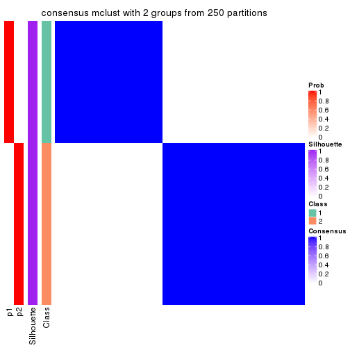
consensus_heatmap(res, k = 3)
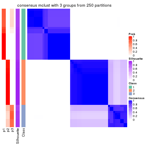
consensus_heatmap(res, k = 4)
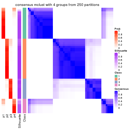
consensus_heatmap(res, k = 5)
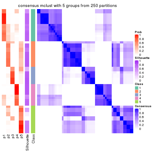
consensus_heatmap(res, k = 6)
Heatmaps for the membership of samples in all partitions to see how consistent they are:
membership_heatmap(res, k = 2)

membership_heatmap(res, k = 3)
membership_heatmap(res, k = 4)
membership_heatmap(res, k = 5)
membership_heatmap(res, k = 6)
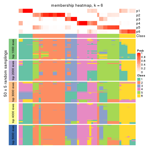
As soon as we have had the classes for columns, we can look for signatures which are significantly different between classes which can be candidate marks for certain classes. Following are the heatmaps for signatures.
Signature heatmaps where rows are scaled:
get_signatures(res, k = 2)

get_signatures(res, k = 3)
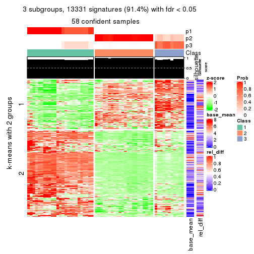
get_signatures(res, k = 4)
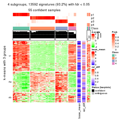
get_signatures(res, k = 5)
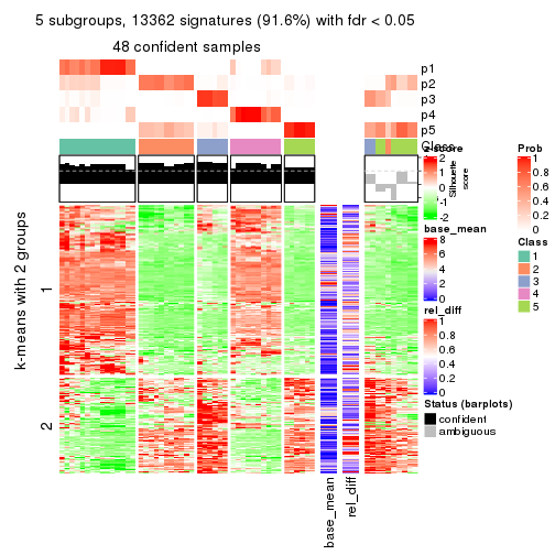
get_signatures(res, k = 6)
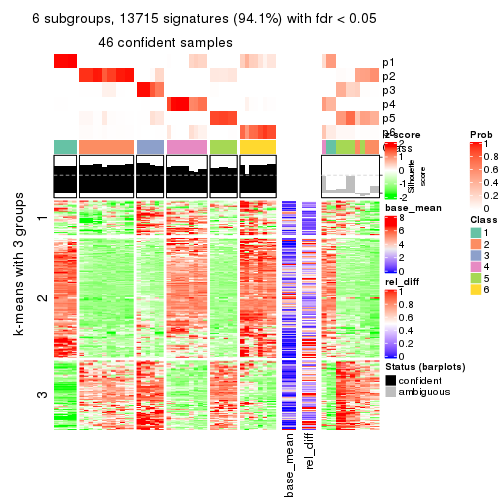
Signature heatmaps where rows are not scaled:
get_signatures(res, k = 2, scale_rows = FALSE)

get_signatures(res, k = 3, scale_rows = FALSE)
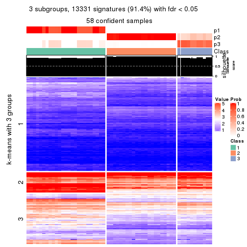
get_signatures(res, k = 4, scale_rows = FALSE)
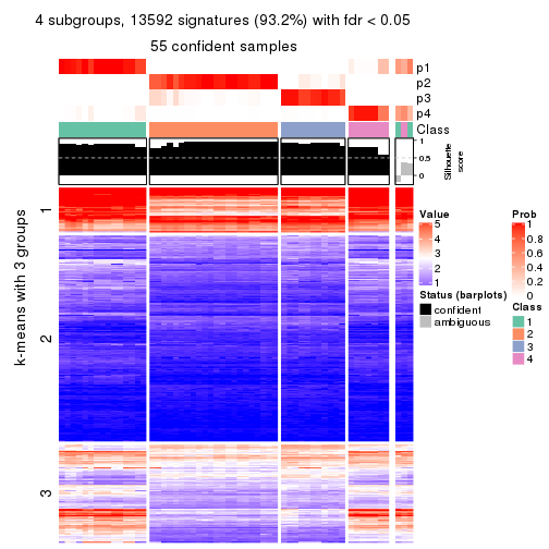
get_signatures(res, k = 5, scale_rows = FALSE)
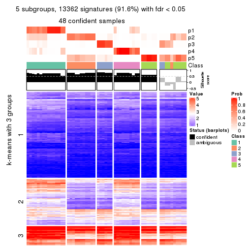
get_signatures(res, k = 6, scale_rows = FALSE)
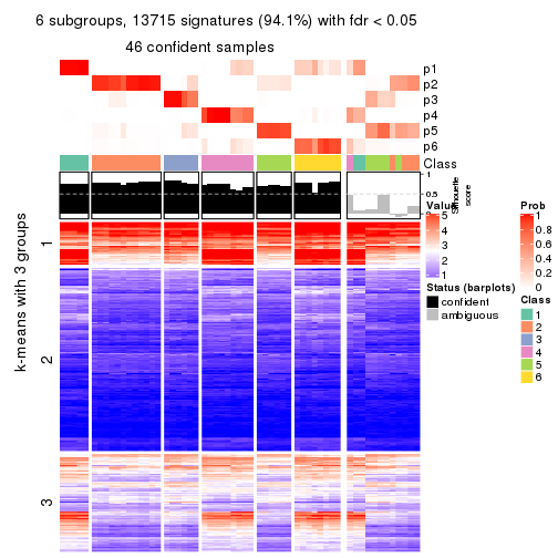
Compare the overlap of signatures from different k:
compare_signatures(res)
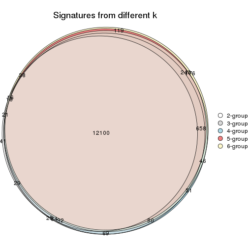
get_signature() returns a data frame invisibly. TO get the list of signatures, the function
call should be assigned to a variable explicitly. In following code, if plot argument is set
to FALSE, no heatmap is plotted while only the differential analysis is performed.
# code only for demonstration
tb = get_signature(res, k = ..., plot = FALSE)
An example of the output of tb is:
#> which_row fdr mean_1 mean_2 scaled_mean_1 scaled_mean_2 km
#> 1 38 0.042760348 8.373488 9.131774 -0.5533452 0.5164555 1
#> 2 40 0.018707592 7.106213 8.469186 -0.6173731 0.5762149 1
#> 3 55 0.019134737 10.221463 11.207825 -0.6159697 0.5749050 1
#> 4 59 0.006059896 5.921854 7.869574 -0.6899429 0.6439467 1
#> 5 60 0.018055526 8.928898 10.211722 -0.6204761 0.5791110 1
#> 6 98 0.009384629 15.714769 14.887706 0.6635654 -0.6193277 2
...
The columns in tb are:
which_row: row indices corresponding to the input matrix.fdr: FDR for the differential test. mean_x: The mean value in group x.scaled_mean_x: The mean value in group x after rows are scaled.km: Row groups if k-means clustering is applied to rows.UMAP plot which shows how samples are separated.
dimension_reduction(res, k = 2, method = "UMAP")
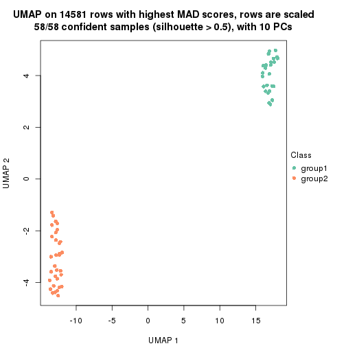
dimension_reduction(res, k = 3, method = "UMAP")

dimension_reduction(res, k = 4, method = "UMAP")
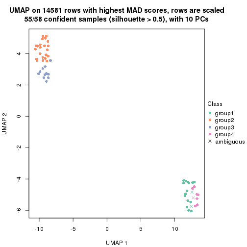
dimension_reduction(res, k = 5, method = "UMAP")
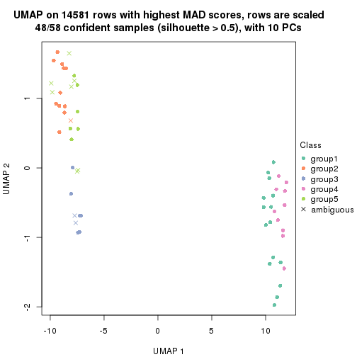
dimension_reduction(res, k = 6, method = "UMAP")
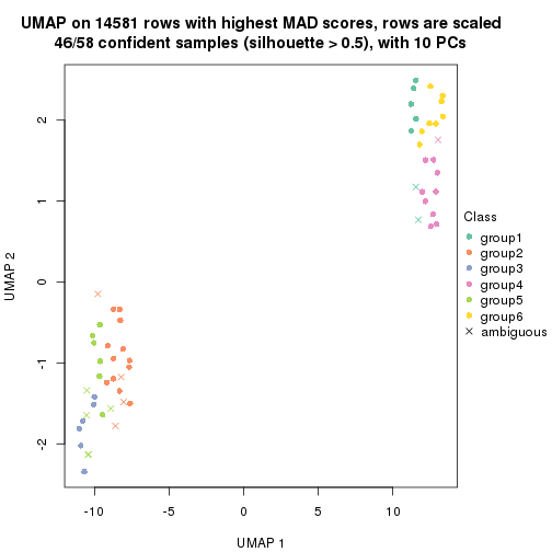
Following heatmap shows how subgroups are split when increasing k:
collect_classes(res)
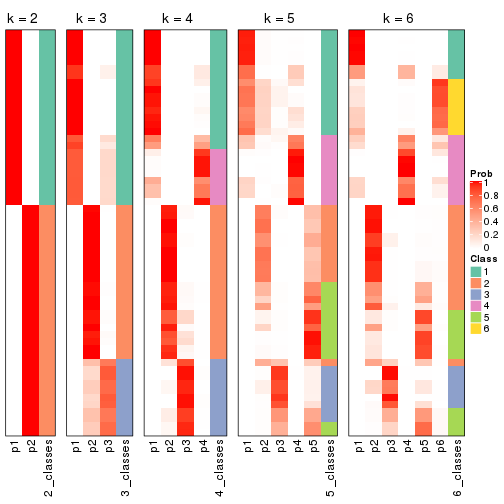
If matrix rows can be associated to genes, consider to use functional_enrichment(res,
...) to perform function enrichment for the signature genes. See this vignette for more detailed explanations.
The object with results only for a single top-value method and a single partition method can be extracted as:
res = res_list["MAD", "NMF"]
# you can also extract it by
# res = res_list["MAD:NMF"]
A summary of res and all the functions that can be applied to it:
res
#> A 'ConsensusPartition' object with k = 2, 3, 4, 5, 6.
#> On a matrix with 14581 rows and 58 columns.
#> Top rows (1000, 2000, 3000, 4000, 5000) are extracted by 'MAD' method.
#> Subgroups are detected by 'NMF' method.
#> Performed in total 1250 partitions by row resampling.
#> Best k for subgroups seems to be 4.
#>
#> Following methods can be applied to this 'ConsensusPartition' object:
#> [1] "cola_report" "collect_classes" "collect_plots"
#> [4] "collect_stats" "colnames" "compare_signatures"
#> [7] "consensus_heatmap" "dimension_reduction" "functional_enrichment"
#> [10] "get_anno_col" "get_anno" "get_classes"
#> [13] "get_consensus" "get_matrix" "get_membership"
#> [16] "get_param" "get_signatures" "get_stats"
#> [19] "is_best_k" "is_stable_k" "membership_heatmap"
#> [22] "ncol" "nrow" "plot_ecdf"
#> [25] "rownames" "select_partition_number" "show"
#> [28] "suggest_best_k" "test_to_known_factors"
collect_plots() function collects all the plots made from res for all k (number of partitions)
into one single page to provide an easy and fast comparison between different k.
collect_plots(res)
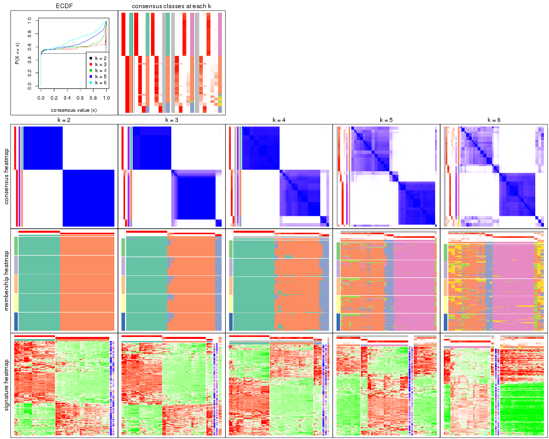
The plots are:
k and the heatmap of
predicted classes for each k.k.k.k.All the plots in panels can be made by individual functions and they are plotted later in this section.
select_partition_number() produces several plots showing different
statistics for choosing “optimized” k. There are following statistics:
k;k, the area increased is defined as \(A_k - A_{k-1}\).The detailed explanations of these statistics can be found in the cola vignette.
Generally speaking, lower PAC score, higher mean silhouette score or higher
concordance corresponds to better partition. Rand index and Jaccard index
measure how similar the current partition is compared to partition with k-1.
If they are too similar, we won't accept k is better than k-1.
select_partition_number(res)
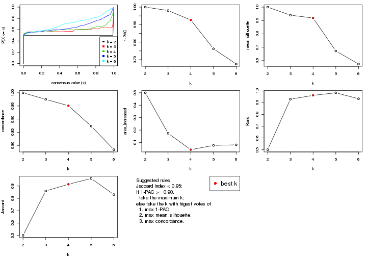
The numeric values for all these statistics can be obtained by get_stats().
get_stats(res)
#> k 1-PAC mean_silhouette concordance area_increased Rand Jaccard
#> 2 2 1.000 1.000 1.000 0.4996 0.501 0.501
#> 3 3 0.980 0.940 0.975 0.1741 0.930 0.860
#> 4 4 0.927 0.919 0.951 0.0425 0.962 0.914
#> 5 5 0.762 0.672 0.874 0.0767 0.984 0.961
#> 6 6 0.675 0.575 0.784 0.0817 0.933 0.831
suggest_best_k() suggests the best \(k\) based on these statistics. The rules are as follows:
suggest_best_k(res)
#> [1] 4
#> attr(,"optional")
#> [1] 2 3
There is also optional best \(k\) = 2 3 that is worth to check.
Following shows the table of the partitions (You need to click the show/hide
code output link to see it). The membership matrix (columns with name p*)
is inferred by
clue::cl_consensus()
function with the SE method. Basically the value in the membership matrix
represents the probability to belong to a certain group. The finall class
label for an item is determined with the group with highest probability it
belongs to.
In get_classes() function, the entropy is calculated from the membership
matrix and the silhouette score is calculated from the consensus matrix.
cbind(get_classes(res, k = 2), get_membership(res, k = 2))
#> class entropy silhouette p1 p2
#> ERR789082 2 0 1 0 1
#> ERR789083 2 0 1 0 1
#> ERR789191 2 0 1 0 1
#> ERR789192 2 0 1 0 1
#> ERR789213 1 0 1 1 0
#> ERR789385 1 0 1 1 0
#> ERR789393 1 0 1 1 0
#> ERR789394 1 0 1 1 0
#> ERR789193 2 0 1 0 1
#> ERR789194 2 0 1 0 1
#> ERR789195 2 0 1 0 1
#> ERR789196 2 0 1 0 1
#> ERR789388 1 0 1 1 0
#> ERR789197 2 0 1 0 1
#> ERR789198 2 0 1 0 1
#> ERR789214 1 0 1 1 0
#> ERR789397 1 0 1 1 0
#> ERR789398 1 0 1 1 0
#> ERR789199 2 0 1 0 1
#> ERR789200 2 0 1 0 1
#> ERR789201 2 0 1 0 1
#> ERR789202 2 0 1 0 1
#> ERR789215 1 0 1 1 0
#> ERR789203 2 0 1 0 1
#> ERR789204 2 0 1 0 1
#> ERR789383 1 0 1 1 0
#> ERR789205 2 0 1 0 1
#> ERR789206 2 0 1 0 1
#> ERR789399 1 0 1 1 0
#> ERR789400 1 0 1 1 0
#> ERR789207 2 0 1 0 1
#> ERR789208 2 0 1 0 1
#> ERR789209 2 0 1 0 1
#> ERR789210 2 0 1 0 1
#> ERR789211 2 0 1 0 1
#> ERR789212 2 0 1 0 1
#> ERR789386 1 0 1 1 0
#> ERR789076 2 0 1 0 1
#> ERR789077 2 0 1 0 1
#> ERR789384 1 0 1 1 0
#> ERR789078 2 0 1 0 1
#> ERR789079 2 0 1 0 1
#> ERR789216 1 0 1 1 0
#> ERR789080 2 0 1 0 1
#> ERR789387 1 0 1 1 0
#> ERR789081 2 0 1 0 1
#> ERR789064 2 0 1 0 1
#> ERR779485 2 0 1 0 1
#> ERR789065 2 0 1 0 1
#> ERR789401 1 0 1 1 0
#> ERR789402 1 0 1 1 0
#> ERR789403 1 0 1 1 0
#> ERR789389 1 0 1 1 0
#> ERR789395 1 0 1 1 0
#> ERR789396 1 0 1 1 0
#> ERR789390 1 0 1 1 0
#> ERR789391 1 0 1 1 0
#> ERR789392 1 0 1 1 0
cbind(get_classes(res, k = 3), get_membership(res, k = 3))
#> class entropy silhouette p1 p2 p3
#> ERR789082 2 0.0000 0.951 0.000 1.000 0.000
#> ERR789083 2 0.0000 0.951 0.000 1.000 0.000
#> ERR789191 2 0.0000 0.951 0.000 1.000 0.000
#> ERR789192 2 0.0000 0.951 0.000 1.000 0.000
#> ERR789213 1 0.0747 0.987 0.984 0.000 0.016
#> ERR789385 1 0.0592 0.990 0.988 0.000 0.012
#> ERR789393 1 0.0592 0.990 0.988 0.000 0.012
#> ERR789394 1 0.0592 0.990 0.988 0.000 0.012
#> ERR789193 3 0.0237 0.981 0.000 0.004 0.996
#> ERR789194 3 0.0237 0.981 0.000 0.004 0.996
#> ERR789195 2 0.6260 0.240 0.000 0.552 0.448
#> ERR789196 2 0.6252 0.252 0.000 0.556 0.444
#> ERR789388 1 0.0000 0.997 1.000 0.000 0.000
#> ERR789197 2 0.0000 0.951 0.000 1.000 0.000
#> ERR789198 2 0.0000 0.951 0.000 1.000 0.000
#> ERR789214 1 0.0000 0.997 1.000 0.000 0.000
#> ERR789397 1 0.0000 0.997 1.000 0.000 0.000
#> ERR789398 1 0.0000 0.997 1.000 0.000 0.000
#> ERR789199 2 0.0000 0.951 0.000 1.000 0.000
#> ERR789200 2 0.0000 0.951 0.000 1.000 0.000
#> ERR789201 2 0.0000 0.951 0.000 1.000 0.000
#> ERR789202 2 0.0000 0.951 0.000 1.000 0.000
#> ERR789215 1 0.0000 0.997 1.000 0.000 0.000
#> ERR789203 2 0.5138 0.666 0.000 0.748 0.252
#> ERR789204 2 0.3879 0.800 0.000 0.848 0.152
#> ERR789383 1 0.0000 0.997 1.000 0.000 0.000
#> ERR789205 2 0.0000 0.951 0.000 1.000 0.000
#> ERR789206 2 0.0000 0.951 0.000 1.000 0.000
#> ERR789399 1 0.0000 0.997 1.000 0.000 0.000
#> ERR789400 1 0.0000 0.997 1.000 0.000 0.000
#> ERR789207 2 0.0000 0.951 0.000 1.000 0.000
#> ERR789208 2 0.0000 0.951 0.000 1.000 0.000
#> ERR789209 2 0.0000 0.951 0.000 1.000 0.000
#> ERR789210 2 0.0000 0.951 0.000 1.000 0.000
#> ERR789211 2 0.0000 0.951 0.000 1.000 0.000
#> ERR789212 2 0.0000 0.951 0.000 1.000 0.000
#> ERR789386 1 0.0000 0.997 1.000 0.000 0.000
#> ERR789076 2 0.0747 0.938 0.000 0.984 0.016
#> ERR789077 2 0.0000 0.951 0.000 1.000 0.000
#> ERR789384 1 0.0000 0.997 1.000 0.000 0.000
#> ERR789078 2 0.0000 0.951 0.000 1.000 0.000
#> ERR789079 2 0.0000 0.951 0.000 1.000 0.000
#> ERR789216 1 0.0000 0.997 1.000 0.000 0.000
#> ERR789080 2 0.0000 0.951 0.000 1.000 0.000
#> ERR789387 1 0.0000 0.997 1.000 0.000 0.000
#> ERR789081 2 0.0000 0.951 0.000 1.000 0.000
#> ERR789064 2 0.0000 0.951 0.000 1.000 0.000
#> ERR779485 3 0.0592 0.980 0.000 0.012 0.988
#> ERR789065 3 0.1753 0.952 0.000 0.048 0.952
#> ERR789401 1 0.0000 0.997 1.000 0.000 0.000
#> ERR789402 1 0.0000 0.997 1.000 0.000 0.000
#> ERR789403 1 0.0000 0.997 1.000 0.000 0.000
#> ERR789389 1 0.0000 0.997 1.000 0.000 0.000
#> ERR789395 1 0.0000 0.997 1.000 0.000 0.000
#> ERR789396 1 0.0000 0.997 1.000 0.000 0.000
#> ERR789390 1 0.0000 0.997 1.000 0.000 0.000
#> ERR789391 1 0.0000 0.997 1.000 0.000 0.000
#> ERR789392 1 0.0592 0.990 0.988 0.000 0.012
cbind(get_classes(res, k = 4), get_membership(res, k = 4))
#> class entropy silhouette p1 p2 p3 p4
#> ERR789082 2 0.0817 0.934 0.000 0.976 0.000 NA
#> ERR789083 2 0.0817 0.934 0.000 0.976 0.000 NA
#> ERR789191 2 0.0817 0.934 0.000 0.976 0.000 NA
#> ERR789192 2 0.0817 0.934 0.000 0.976 0.000 NA
#> ERR789213 1 0.2032 0.951 0.936 0.000 0.036 NA
#> ERR789385 1 0.1042 0.979 0.972 0.000 0.008 NA
#> ERR789393 1 0.0895 0.982 0.976 0.000 0.004 NA
#> ERR789394 1 0.0895 0.982 0.976 0.000 0.004 NA
#> ERR789193 3 0.0592 0.834 0.000 0.000 0.984 NA
#> ERR789194 3 0.0592 0.834 0.000 0.000 0.984 NA
#> ERR789195 2 0.4868 0.644 0.000 0.720 0.256 NA
#> ERR789196 2 0.4609 0.701 0.000 0.752 0.224 NA
#> ERR789388 1 0.0336 0.990 0.992 0.000 0.000 NA
#> ERR789197 2 0.0817 0.934 0.000 0.976 0.000 NA
#> ERR789198 2 0.0817 0.934 0.000 0.976 0.000 NA
#> ERR789214 1 0.0469 0.989 0.988 0.000 0.000 NA
#> ERR789397 1 0.0469 0.989 0.988 0.000 0.000 NA
#> ERR789398 1 0.0469 0.989 0.988 0.000 0.000 NA
#> ERR789199 2 0.0921 0.933 0.000 0.972 0.000 NA
#> ERR789200 2 0.0921 0.933 0.000 0.972 0.000 NA
#> ERR789201 2 0.0336 0.934 0.000 0.992 0.008 NA
#> ERR789202 2 0.0336 0.934 0.000 0.992 0.008 NA
#> ERR789215 1 0.0336 0.990 0.992 0.000 0.000 NA
#> ERR789203 3 0.6033 0.560 0.000 0.316 0.620 NA
#> ERR789204 3 0.6186 0.488 0.000 0.352 0.584 NA
#> ERR789383 1 0.0469 0.987 0.988 0.000 0.000 NA
#> ERR789205 2 0.2198 0.917 0.000 0.920 0.008 NA
#> ERR789206 2 0.2124 0.919 0.000 0.924 0.008 NA
#> ERR789399 1 0.0336 0.990 0.992 0.000 0.000 NA
#> ERR789400 1 0.0336 0.990 0.992 0.000 0.000 NA
#> ERR789207 2 0.0524 0.933 0.000 0.988 0.008 NA
#> ERR789208 2 0.0524 0.933 0.000 0.988 0.008 NA
#> ERR789209 2 0.2198 0.909 0.000 0.920 0.008 NA
#> ERR789210 2 0.2342 0.904 0.000 0.912 0.008 NA
#> ERR789211 2 0.1890 0.917 0.000 0.936 0.008 NA
#> ERR789212 2 0.1807 0.919 0.000 0.940 0.008 NA
#> ERR789386 1 0.0336 0.990 0.992 0.000 0.000 NA
#> ERR789076 2 0.2319 0.904 0.000 0.924 0.040 NA
#> ERR789077 2 0.0188 0.933 0.000 0.996 0.000 NA
#> ERR789384 1 0.0000 0.991 1.000 0.000 0.000 NA
#> ERR789078 2 0.0188 0.933 0.000 0.996 0.000 NA
#> ERR789079 2 0.1211 0.920 0.000 0.960 0.000 NA
#> ERR789216 1 0.0188 0.991 0.996 0.000 0.000 NA
#> ERR789080 2 0.3610 0.761 0.000 0.800 0.000 NA
#> ERR789387 1 0.0336 0.989 0.992 0.000 0.000 NA
#> ERR789081 2 0.3219 0.807 0.000 0.836 0.000 NA
#> ERR789064 2 0.0188 0.933 0.000 0.996 0.000 NA
#> ERR779485 3 0.0188 0.834 0.000 0.000 0.996 NA
#> ERR789065 3 0.1022 0.830 0.000 0.032 0.968 NA
#> ERR789401 1 0.0000 0.991 1.000 0.000 0.000 NA
#> ERR789402 1 0.0000 0.991 1.000 0.000 0.000 NA
#> ERR789403 1 0.0000 0.991 1.000 0.000 0.000 NA
#> ERR789389 1 0.0336 0.989 0.992 0.000 0.000 NA
#> ERR789395 1 0.0000 0.991 1.000 0.000 0.000 NA
#> ERR789396 1 0.0000 0.991 1.000 0.000 0.000 NA
#> ERR789390 1 0.0188 0.991 0.996 0.000 0.000 NA
#> ERR789391 1 0.0188 0.991 0.996 0.000 0.000 NA
#> ERR789392 1 0.0895 0.982 0.976 0.000 0.004 NA
cbind(get_classes(res, k = 5), get_membership(res, k = 5))
#> class entropy silhouette p1 p2 p3 p4 p5
#> ERR789082 2 0.0579 0.6147 NA 0.984 0.000 0.000 0.008
#> ERR789083 2 0.0579 0.6147 NA 0.984 0.000 0.000 0.008
#> ERR789191 2 0.0566 0.6152 NA 0.984 0.000 0.000 0.004
#> ERR789192 2 0.0566 0.6152 NA 0.984 0.000 0.000 0.004
#> ERR789213 4 0.4262 0.7856 NA 0.000 0.124 0.776 0.000
#> ERR789385 4 0.2754 0.9015 NA 0.000 0.040 0.880 0.000
#> ERR789393 4 0.1956 0.9304 NA 0.000 0.008 0.916 0.000
#> ERR789394 4 0.1956 0.9304 NA 0.000 0.008 0.916 0.000
#> ERR789193 3 0.0703 0.7628 NA 0.000 0.976 0.000 0.000
#> ERR789194 3 0.0794 0.7608 NA 0.000 0.972 0.000 0.000
#> ERR789195 2 0.4914 0.1612 NA 0.672 0.284 0.000 0.016
#> ERR789196 2 0.4681 0.2032 NA 0.692 0.272 0.000 0.016
#> ERR789388 4 0.0290 0.9682 NA 0.000 0.000 0.992 0.000
#> ERR789197 2 0.1200 0.6084 NA 0.964 0.016 0.000 0.008
#> ERR789198 2 0.1095 0.6107 NA 0.968 0.012 0.000 0.008
#> ERR789214 4 0.0404 0.9678 NA 0.000 0.000 0.988 0.000
#> ERR789397 4 0.0404 0.9686 NA 0.000 0.000 0.988 0.000
#> ERR789398 4 0.0404 0.9686 NA 0.000 0.000 0.988 0.000
#> ERR789199 2 0.0703 0.6140 NA 0.976 0.000 0.000 0.000
#> ERR789200 2 0.0703 0.6140 NA 0.976 0.000 0.000 0.000
#> ERR789201 2 0.2747 0.6117 NA 0.884 0.012 0.000 0.088
#> ERR789202 2 0.2844 0.6116 NA 0.880 0.012 0.000 0.088
#> ERR789215 4 0.0771 0.9648 NA 0.000 0.000 0.976 0.004
#> ERR789203 3 0.7749 0.4219 NA 0.212 0.464 0.000 0.228
#> ERR789204 3 0.7769 0.4024 NA 0.224 0.460 0.000 0.220
#> ERR789383 4 0.0794 0.9642 NA 0.000 0.000 0.972 0.000
#> ERR789205 2 0.5235 0.3658 NA 0.728 0.040 0.000 0.160
#> ERR789206 2 0.5093 0.3857 NA 0.736 0.040 0.000 0.164
#> ERR789399 4 0.0703 0.9660 NA 0.000 0.000 0.976 0.000
#> ERR789400 4 0.0703 0.9660 NA 0.000 0.000 0.976 0.000
#> ERR789207 2 0.3048 0.5519 NA 0.820 0.004 0.000 0.176
#> ERR789208 2 0.2970 0.5567 NA 0.828 0.004 0.000 0.168
#> ERR789209 2 0.4602 0.3499 NA 0.640 0.016 0.000 0.340
#> ERR789210 2 0.4647 0.3208 NA 0.628 0.016 0.000 0.352
#> ERR789211 2 0.3980 0.4623 NA 0.708 0.008 0.000 0.284
#> ERR789212 2 0.4003 0.4557 NA 0.704 0.008 0.000 0.288
#> ERR789386 4 0.0290 0.9687 NA 0.000 0.000 0.992 0.000
#> ERR789076 2 0.6258 -0.0113 NA 0.592 0.156 0.000 0.236
#> ERR789077 2 0.3128 0.5357 NA 0.824 0.004 0.000 0.168
#> ERR789384 4 0.0992 0.9622 NA 0.000 0.008 0.968 0.000
#> ERR789078 2 0.3317 0.5082 NA 0.804 0.004 0.000 0.188
#> ERR789079 2 0.3844 0.3078 NA 0.736 0.004 0.000 0.256
#> ERR789216 4 0.0510 0.9684 NA 0.000 0.000 0.984 0.000
#> ERR789080 5 0.5234 0.0000 NA 0.460 0.000 0.000 0.496
#> ERR789387 4 0.0609 0.9673 NA 0.000 0.000 0.980 0.000
#> ERR789081 2 0.4947 -0.5620 NA 0.576 0.004 0.000 0.396
#> ERR789064 2 0.2763 0.5602 NA 0.848 0.004 0.000 0.148
#> ERR779485 3 0.0703 0.7670 NA 0.000 0.976 0.000 0.024
#> ERR789065 3 0.1661 0.7554 NA 0.036 0.940 0.000 0.024
#> ERR789401 4 0.0404 0.9683 NA 0.000 0.000 0.988 0.000
#> ERR789402 4 0.0404 0.9683 NA 0.000 0.000 0.988 0.000
#> ERR789403 4 0.0404 0.9683 NA 0.000 0.000 0.988 0.000
#> ERR789389 4 0.0404 0.9689 NA 0.000 0.000 0.988 0.000
#> ERR789395 4 0.0404 0.9683 NA 0.000 0.000 0.988 0.000
#> ERR789396 4 0.0510 0.9676 NA 0.000 0.000 0.984 0.000
#> ERR789390 4 0.0404 0.9688 NA 0.000 0.000 0.988 0.000
#> ERR789391 4 0.0404 0.9688 NA 0.000 0.000 0.988 0.000
#> ERR789392 4 0.1894 0.9330 NA 0.000 0.008 0.920 0.000
cbind(get_classes(res, k = 6), get_membership(res, k = 6))
#> class entropy silhouette p1 p2 p3 p4 p5 p6
#> ERR789082 2 0.2611 0.4743 NA 0.876 0.008 0.000 0.016 0.004
#> ERR789083 2 0.2567 0.4726 NA 0.876 0.008 0.000 0.012 0.004
#> ERR789191 2 0.2567 0.4701 NA 0.876 0.008 0.000 0.012 0.004
#> ERR789192 2 0.2662 0.4635 NA 0.868 0.008 0.000 0.012 0.004
#> ERR789213 4 0.4003 0.7937 NA 0.000 0.116 0.760 0.000 0.000
#> ERR789385 4 0.3297 0.8549 NA 0.000 0.068 0.820 0.000 0.000
#> ERR789393 4 0.2199 0.9141 NA 0.000 0.020 0.892 0.000 0.000
#> ERR789394 4 0.2333 0.9094 NA 0.000 0.024 0.884 0.000 0.000
#> ERR789193 3 0.0951 0.7021 NA 0.004 0.968 0.000 0.000 0.008
#> ERR789194 3 0.0922 0.6993 NA 0.004 0.968 0.000 0.000 0.004
#> ERR789195 3 0.6445 -0.0414 NA 0.420 0.432 0.000 0.028 0.084
#> ERR789196 2 0.6418 -0.1607 NA 0.448 0.404 0.000 0.028 0.088
#> ERR789388 4 0.0665 0.9400 NA 0.000 0.004 0.980 0.000 0.008
#> ERR789197 2 0.3383 0.4972 NA 0.856 0.032 0.000 0.036 0.052
#> ERR789198 2 0.3378 0.4968 NA 0.856 0.028 0.000 0.040 0.052
#> ERR789214 4 0.1149 0.9380 NA 0.000 0.008 0.960 0.000 0.008
#> ERR789397 4 0.0862 0.9391 NA 0.000 0.008 0.972 0.000 0.004
#> ERR789398 4 0.0862 0.9391 NA 0.000 0.008 0.972 0.000 0.004
#> ERR789199 2 0.4388 0.4406 NA 0.776 0.004 0.000 0.092 0.048
#> ERR789200 2 0.4230 0.4498 NA 0.788 0.004 0.000 0.092 0.048
#> ERR789201 2 0.4117 0.4086 NA 0.708 0.004 0.000 0.028 0.256
#> ERR789202 2 0.4022 0.4244 NA 0.724 0.004 0.000 0.028 0.240
#> ERR789215 4 0.0820 0.9414 NA 0.000 0.000 0.972 0.000 0.016
#> ERR789203 6 0.5800 0.1720 NA 0.144 0.328 0.000 0.012 0.516
#> ERR789204 6 0.6038 0.1812 NA 0.160 0.328 0.000 0.012 0.496
#> ERR789383 4 0.1934 0.9298 NA 0.000 0.000 0.916 0.000 0.040
#> ERR789205 2 0.6021 -0.0424 NA 0.472 0.088 0.000 0.016 0.404
#> ERR789206 2 0.5979 -0.0262 NA 0.480 0.084 0.000 0.016 0.400
#> ERR789399 4 0.1408 0.9343 NA 0.000 0.000 0.944 0.000 0.036
#> ERR789400 4 0.1408 0.9343 NA 0.000 0.000 0.944 0.000 0.036
#> ERR789207 2 0.4775 0.3344 NA 0.688 0.004 0.000 0.152 0.156
#> ERR789208 2 0.4741 0.3358 NA 0.692 0.004 0.000 0.152 0.152
#> ERR789209 6 0.6207 0.1497 NA 0.412 0.024 0.000 0.136 0.424
#> ERR789210 6 0.6231 0.1498 NA 0.408 0.024 0.000 0.140 0.424
#> ERR789211 2 0.6020 -0.1165 NA 0.504 0.016 0.000 0.144 0.332
#> ERR789212 2 0.5992 -0.1098 NA 0.508 0.016 0.000 0.140 0.332
#> ERR789386 4 0.1003 0.9376 NA 0.000 0.004 0.964 0.000 0.004
#> ERR789076 2 0.7148 -0.2389 NA 0.364 0.280 0.000 0.288 0.064
#> ERR789077 2 0.3171 0.3224 NA 0.784 0.000 0.000 0.204 0.012
#> ERR789384 4 0.2118 0.9320 NA 0.000 0.020 0.916 0.004 0.012
#> ERR789078 2 0.3705 0.2546 NA 0.740 0.004 0.000 0.236 0.020
#> ERR789079 2 0.3634 -0.1331 NA 0.644 0.000 0.000 0.356 0.000
#> ERR789216 4 0.1410 0.9348 NA 0.000 0.000 0.944 0.004 0.008
#> ERR789080 5 0.3767 0.7519 NA 0.276 0.000 0.000 0.708 0.004
#> ERR789387 4 0.1523 0.9352 NA 0.000 0.000 0.940 0.008 0.008
#> ERR789081 5 0.3915 0.7104 NA 0.412 0.000 0.000 0.584 0.004
#> ERR789064 2 0.2494 0.4361 NA 0.864 0.000 0.000 0.120 0.016
#> ERR779485 3 0.2274 0.6857 NA 0.012 0.892 0.000 0.008 0.088
#> ERR789065 3 0.3463 0.6372 NA 0.080 0.832 0.000 0.024 0.064
#> ERR789401 4 0.2003 0.9284 NA 0.000 0.000 0.912 0.000 0.044
#> ERR789402 4 0.2001 0.9278 NA 0.000 0.000 0.912 0.000 0.040
#> ERR789403 4 0.2003 0.9284 NA 0.000 0.000 0.912 0.000 0.044
#> ERR789389 4 0.1642 0.9398 NA 0.000 0.000 0.936 0.004 0.032
#> ERR789395 4 0.2001 0.9278 NA 0.000 0.000 0.912 0.000 0.040
#> ERR789396 4 0.2001 0.9278 NA 0.000 0.000 0.912 0.000 0.040
#> ERR789390 4 0.0820 0.9410 NA 0.000 0.000 0.972 0.000 0.012
#> ERR789391 4 0.0820 0.9410 NA 0.000 0.000 0.972 0.000 0.012
#> ERR789392 4 0.2250 0.9118 NA 0.000 0.020 0.888 0.000 0.000
Heatmaps for the consensus matrix. It visualizes the probability of two samples to be in a same group.
consensus_heatmap(res, k = 2)

consensus_heatmap(res, k = 3)
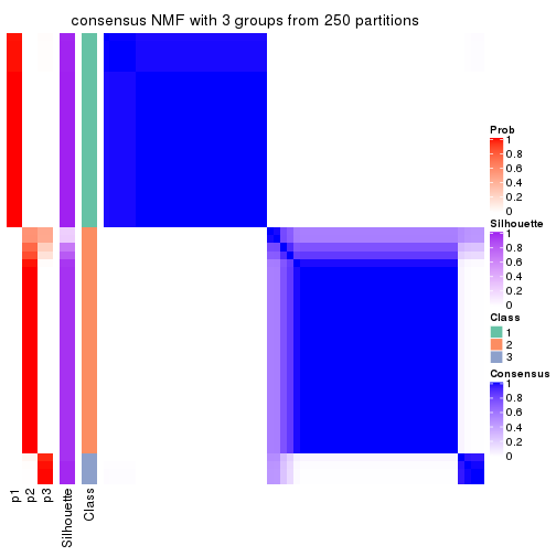
consensus_heatmap(res, k = 4)
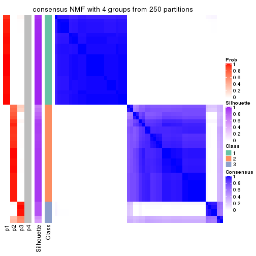
consensus_heatmap(res, k = 5)
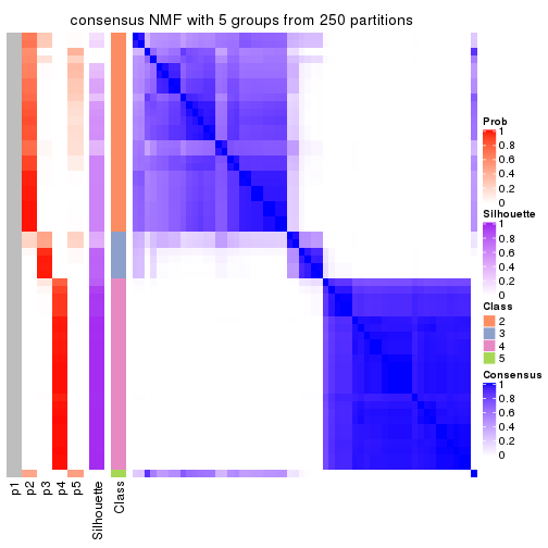
consensus_heatmap(res, k = 6)
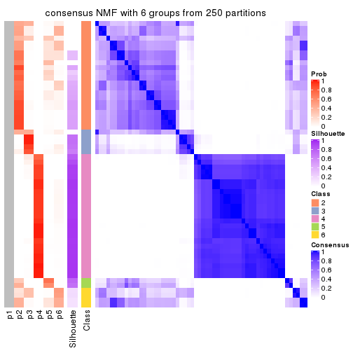
Heatmaps for the membership of samples in all partitions to see how consistent they are:
membership_heatmap(res, k = 2)

membership_heatmap(res, k = 3)
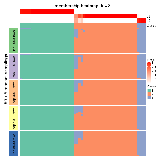
membership_heatmap(res, k = 4)

membership_heatmap(res, k = 5)
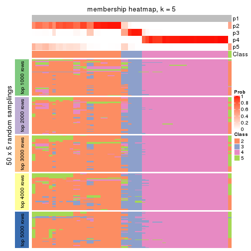
membership_heatmap(res, k = 6)
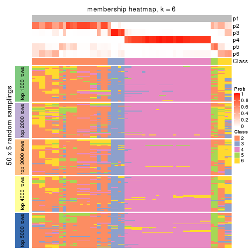
As soon as we have had the classes for columns, we can look for signatures which are significantly different between classes which can be candidate marks for certain classes. Following are the heatmaps for signatures.
Signature heatmaps where rows are scaled:
get_signatures(res, k = 2)

get_signatures(res, k = 3)
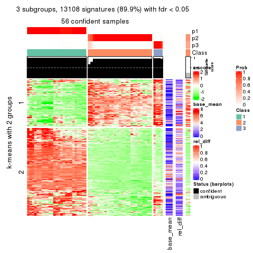
get_signatures(res, k = 4)
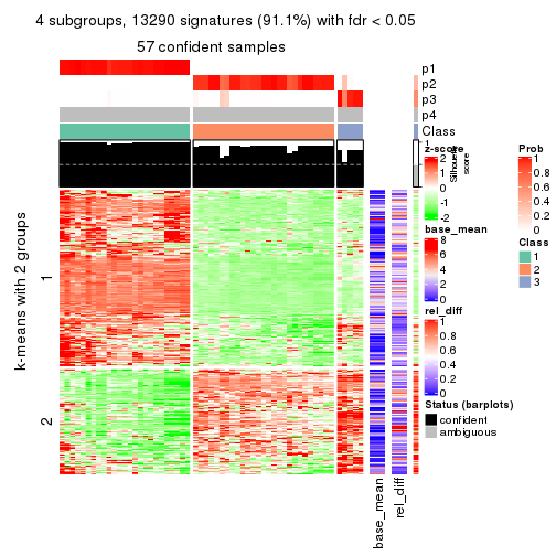
get_signatures(res, k = 5)
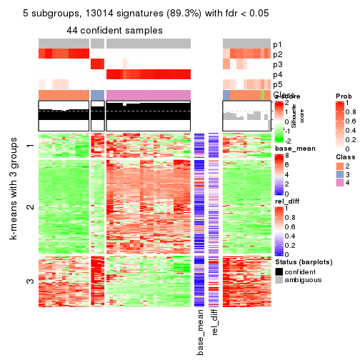
get_signatures(res, k = 6)
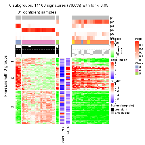
Signature heatmaps where rows are not scaled:
get_signatures(res, k = 2, scale_rows = FALSE)

get_signatures(res, k = 3, scale_rows = FALSE)
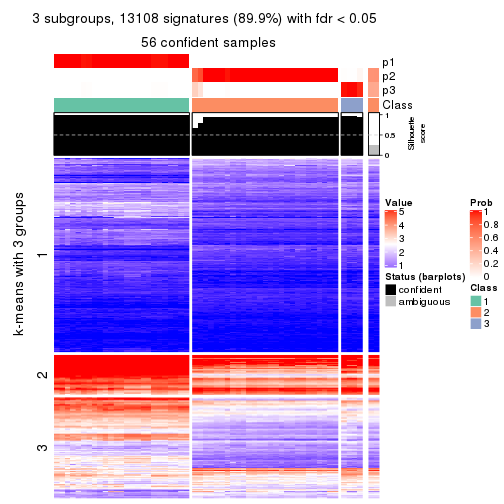
get_signatures(res, k = 4, scale_rows = FALSE)
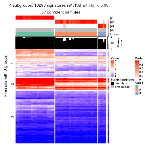
get_signatures(res, k = 5, scale_rows = FALSE)
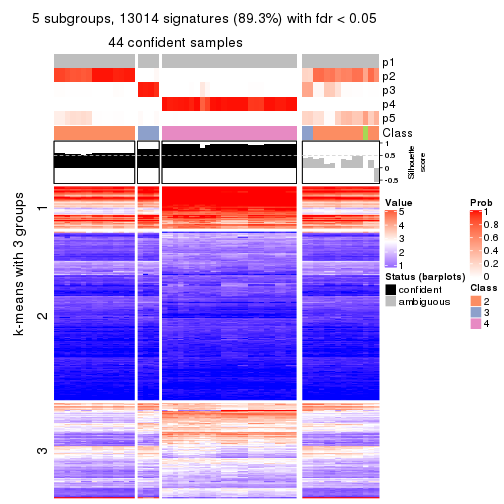
get_signatures(res, k = 6, scale_rows = FALSE)
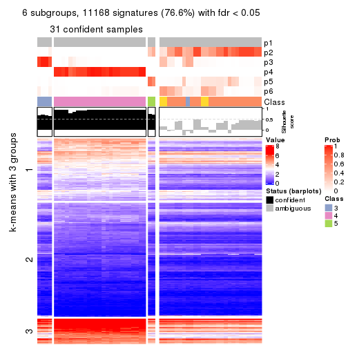
Compare the overlap of signatures from different k:
compare_signatures(res)
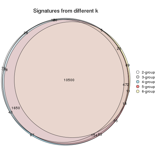
get_signature() returns a data frame invisibly. TO get the list of signatures, the function
call should be assigned to a variable explicitly. In following code, if plot argument is set
to FALSE, no heatmap is plotted while only the differential analysis is performed.
# code only for demonstration
tb = get_signature(res, k = ..., plot = FALSE)
An example of the output of tb is:
#> which_row fdr mean_1 mean_2 scaled_mean_1 scaled_mean_2 km
#> 1 38 0.042760348 8.373488 9.131774 -0.5533452 0.5164555 1
#> 2 40 0.018707592 7.106213 8.469186 -0.6173731 0.5762149 1
#> 3 55 0.019134737 10.221463 11.207825 -0.6159697 0.5749050 1
#> 4 59 0.006059896 5.921854 7.869574 -0.6899429 0.6439467 1
#> 5 60 0.018055526 8.928898 10.211722 -0.6204761 0.5791110 1
#> 6 98 0.009384629 15.714769 14.887706 0.6635654 -0.6193277 2
...
The columns in tb are:
which_row: row indices corresponding to the input matrix.fdr: FDR for the differential test. mean_x: The mean value in group x.scaled_mean_x: The mean value in group x after rows are scaled.km: Row groups if k-means clustering is applied to rows.UMAP plot which shows how samples are separated.
dimension_reduction(res, k = 2, method = "UMAP")

dimension_reduction(res, k = 3, method = "UMAP")
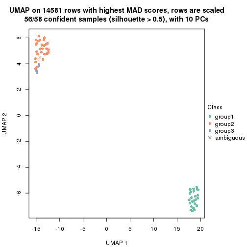
dimension_reduction(res, k = 4, method = "UMAP")

dimension_reduction(res, k = 5, method = "UMAP")
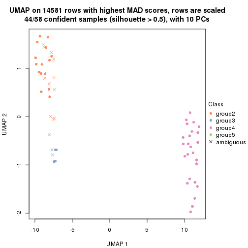
dimension_reduction(res, k = 6, method = "UMAP")
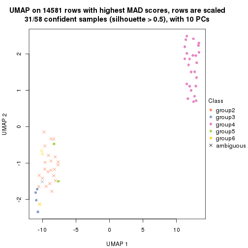
Following heatmap shows how subgroups are split when increasing k:
collect_classes(res)
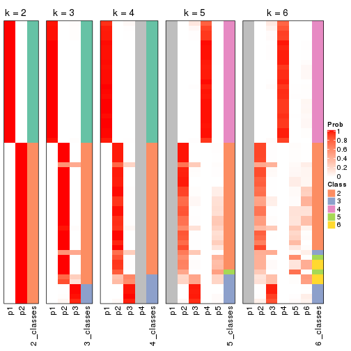
If matrix rows can be associated to genes, consider to use functional_enrichment(res,
...) to perform function enrichment for the signature genes. See this vignette for more detailed explanations.
The object with results only for a single top-value method and a single partition method can be extracted as:
res = res_list["ATC", "hclust"]
# you can also extract it by
# res = res_list["ATC:hclust"]
A summary of res and all the functions that can be applied to it:
res
#> A 'ConsensusPartition' object with k = 2, 3, 4, 5, 6.
#> On a matrix with 14581 rows and 58 columns.
#> Top rows (1000, 2000, 3000, 4000, 5000) are extracted by 'ATC' method.
#> Subgroups are detected by 'hclust' method.
#> Performed in total 1250 partitions by row resampling.
#> Best k for subgroups seems to be 5.
#>
#> Following methods can be applied to this 'ConsensusPartition' object:
#> [1] "cola_report" "collect_classes" "collect_plots"
#> [4] "collect_stats" "colnames" "compare_signatures"
#> [7] "consensus_heatmap" "dimension_reduction" "functional_enrichment"
#> [10] "get_anno_col" "get_anno" "get_classes"
#> [13] "get_consensus" "get_matrix" "get_membership"
#> [16] "get_param" "get_signatures" "get_stats"
#> [19] "is_best_k" "is_stable_k" "membership_heatmap"
#> [22] "ncol" "nrow" "plot_ecdf"
#> [25] "rownames" "select_partition_number" "show"
#> [28] "suggest_best_k" "test_to_known_factors"
collect_plots() function collects all the plots made from res for all k (number of partitions)
into one single page to provide an easy and fast comparison between different k.
collect_plots(res)
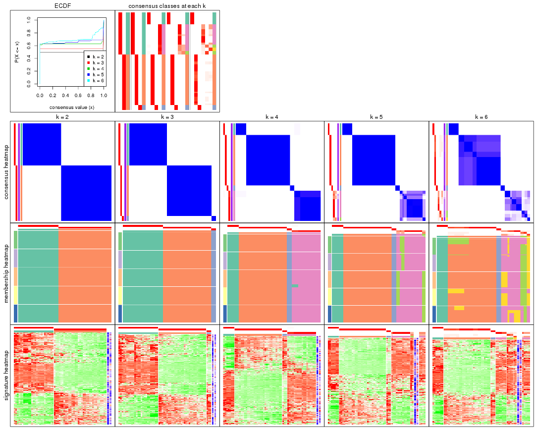
The plots are:
k and the heatmap of
predicted classes for each k.k.k.k.All the plots in panels can be made by individual functions and they are plotted later in this section.
select_partition_number() produces several plots showing different
statistics for choosing “optimized” k. There are following statistics:
k;k, the area increased is defined as \(A_k - A_{k-1}\).The detailed explanations of these statistics can be found in the cola vignette.
Generally speaking, lower PAC score, higher mean silhouette score or higher
concordance corresponds to better partition. Rand index and Jaccard index
measure how similar the current partition is compared to partition with k-1.
If they are too similar, we won't accept k is better than k-1.
select_partition_number(res)
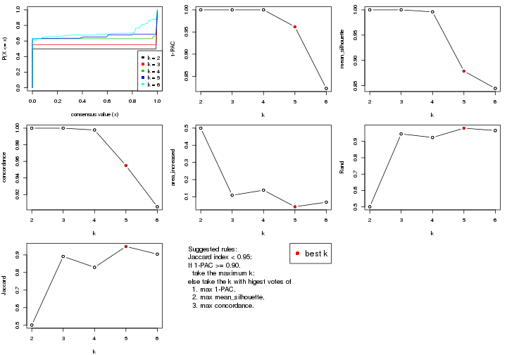
The numeric values for all these statistics can be obtained by get_stats().
get_stats(res)
#> k 1-PAC mean_silhouette concordance area_increased Rand Jaccard
#> 2 2 1.000 1.000 1.000 0.4996 0.501 0.501
#> 3 3 1.000 1.000 1.000 0.1089 0.946 0.891
#> 4 4 1.000 0.996 0.998 0.1384 0.924 0.829
#> 5 5 0.962 0.879 0.955 0.0419 0.981 0.948
#> 6 6 0.823 0.845 0.905 0.0685 0.966 0.904
suggest_best_k() suggests the best \(k\) based on these statistics. The rules are as follows:
suggest_best_k(res)
#> [1] 5
#> attr(,"optional")
#> [1] 2 3 4
There is also optional best \(k\) = 2 3 4 that is worth to check.
Following shows the table of the partitions (You need to click the show/hide
code output link to see it). The membership matrix (columns with name p*)
is inferred by
clue::cl_consensus()
function with the SE method. Basically the value in the membership matrix
represents the probability to belong to a certain group. The finall class
label for an item is determined with the group with highest probability it
belongs to.
In get_classes() function, the entropy is calculated from the membership
matrix and the silhouette score is calculated from the consensus matrix.
cbind(get_classes(res, k = 2), get_membership(res, k = 2))
#> class entropy silhouette p1 p2
#> ERR789082 2 0 1 0 1
#> ERR789083 2 0 1 0 1
#> ERR789191 2 0 1 0 1
#> ERR789192 2 0 1 0 1
#> ERR789213 1 0 1 1 0
#> ERR789385 1 0 1 1 0
#> ERR789393 1 0 1 1 0
#> ERR789394 1 0 1 1 0
#> ERR789193 2 0 1 0 1
#> ERR789194 2 0 1 0 1
#> ERR789195 2 0 1 0 1
#> ERR789196 2 0 1 0 1
#> ERR789388 1 0 1 1 0
#> ERR789197 2 0 1 0 1
#> ERR789198 2 0 1 0 1
#> ERR789214 1 0 1 1 0
#> ERR789397 1 0 1 1 0
#> ERR789398 1 0 1 1 0
#> ERR789199 2 0 1 0 1
#> ERR789200 2 0 1 0 1
#> ERR789201 2 0 1 0 1
#> ERR789202 2 0 1 0 1
#> ERR789215 1 0 1 1 0
#> ERR789203 2 0 1 0 1
#> ERR789204 2 0 1 0 1
#> ERR789383 1 0 1 1 0
#> ERR789205 2 0 1 0 1
#> ERR789206 2 0 1 0 1
#> ERR789399 1 0 1 1 0
#> ERR789400 1 0 1 1 0
#> ERR789207 2 0 1 0 1
#> ERR789208 2 0 1 0 1
#> ERR789209 2 0 1 0 1
#> ERR789210 2 0 1 0 1
#> ERR789211 2 0 1 0 1
#> ERR789212 2 0 1 0 1
#> ERR789386 1 0 1 1 0
#> ERR789076 2 0 1 0 1
#> ERR789077 2 0 1 0 1
#> ERR789384 1 0 1 1 0
#> ERR789078 2 0 1 0 1
#> ERR789079 2 0 1 0 1
#> ERR789216 1 0 1 1 0
#> ERR789080 2 0 1 0 1
#> ERR789387 1 0 1 1 0
#> ERR789081 2 0 1 0 1
#> ERR789064 2 0 1 0 1
#> ERR779485 2 0 1 0 1
#> ERR789065 2 0 1 0 1
#> ERR789401 1 0 1 1 0
#> ERR789402 1 0 1 1 0
#> ERR789403 1 0 1 1 0
#> ERR789389 1 0 1 1 0
#> ERR789395 1 0 1 1 0
#> ERR789396 1 0 1 1 0
#> ERR789390 1 0 1 1 0
#> ERR789391 1 0 1 1 0
#> ERR789392 1 0 1 1 0
cbind(get_classes(res, k = 3), get_membership(res, k = 3))
#> class entropy silhouette p1 p2 p3
#> ERR789082 2 0 1 0 1 0
#> ERR789083 2 0 1 0 1 0
#> ERR789191 2 0 1 0 1 0
#> ERR789192 2 0 1 0 1 0
#> ERR789213 1 0 1 1 0 0
#> ERR789385 1 0 1 1 0 0
#> ERR789393 1 0 1 1 0 0
#> ERR789394 1 0 1 1 0 0
#> ERR789193 3 0 1 0 0 1
#> ERR789194 3 0 1 0 0 1
#> ERR789195 2 0 1 0 1 0
#> ERR789196 2 0 1 0 1 0
#> ERR789388 1 0 1 1 0 0
#> ERR789197 2 0 1 0 1 0
#> ERR789198 2 0 1 0 1 0
#> ERR789214 1 0 1 1 0 0
#> ERR789397 1 0 1 1 0 0
#> ERR789398 1 0 1 1 0 0
#> ERR789199 2 0 1 0 1 0
#> ERR789200 2 0 1 0 1 0
#> ERR789201 2 0 1 0 1 0
#> ERR789202 2 0 1 0 1 0
#> ERR789215 1 0 1 1 0 0
#> ERR789203 2 0 1 0 1 0
#> ERR789204 2 0 1 0 1 0
#> ERR789383 1 0 1 1 0 0
#> ERR789205 2 0 1 0 1 0
#> ERR789206 2 0 1 0 1 0
#> ERR789399 1 0 1 1 0 0
#> ERR789400 1 0 1 1 0 0
#> ERR789207 2 0 1 0 1 0
#> ERR789208 2 0 1 0 1 0
#> ERR789209 2 0 1 0 1 0
#> ERR789210 2 0 1 0 1 0
#> ERR789211 2 0 1 0 1 0
#> ERR789212 2 0 1 0 1 0
#> ERR789386 1 0 1 1 0 0
#> ERR789076 2 0 1 0 1 0
#> ERR789077 2 0 1 0 1 0
#> ERR789384 1 0 1 1 0 0
#> ERR789078 2 0 1 0 1 0
#> ERR789079 2 0 1 0 1 0
#> ERR789216 1 0 1 1 0 0
#> ERR789080 2 0 1 0 1 0
#> ERR789387 1 0 1 1 0 0
#> ERR789081 2 0 1 0 1 0
#> ERR789064 2 0 1 0 1 0
#> ERR779485 3 0 1 0 0 1
#> ERR789065 2 0 1 0 1 0
#> ERR789401 1 0 1 1 0 0
#> ERR789402 1 0 1 1 0 0
#> ERR789403 1 0 1 1 0 0
#> ERR789389 1 0 1 1 0 0
#> ERR789395 1 0 1 1 0 0
#> ERR789396 1 0 1 1 0 0
#> ERR789390 1 0 1 1 0 0
#> ERR789391 1 0 1 1 0 0
#> ERR789392 1 0 1 1 0 0
cbind(get_classes(res, k = 4), get_membership(res, k = 4))
#> class entropy silhouette p1 p2 p3 p4
#> ERR789082 2 0.000 1.000 0.000 1 0 0.000
#> ERR789083 2 0.000 1.000 0.000 1 0 0.000
#> ERR789191 2 0.000 1.000 0.000 1 0 0.000
#> ERR789192 2 0.000 1.000 0.000 1 0 0.000
#> ERR789213 4 0.000 0.992 0.000 0 0 1.000
#> ERR789385 4 0.000 0.992 0.000 0 0 1.000
#> ERR789393 4 0.000 0.992 0.000 0 0 1.000
#> ERR789394 4 0.000 0.992 0.000 0 0 1.000
#> ERR789193 3 0.000 1.000 0.000 0 1 0.000
#> ERR789194 3 0.000 1.000 0.000 0 1 0.000
#> ERR789195 2 0.000 1.000 0.000 1 0 0.000
#> ERR789196 2 0.000 1.000 0.000 1 0 0.000
#> ERR789388 4 0.000 0.992 0.000 0 0 1.000
#> ERR789197 2 0.000 1.000 0.000 1 0 0.000
#> ERR789198 2 0.000 1.000 0.000 1 0 0.000
#> ERR789214 4 0.000 0.992 0.000 0 0 1.000
#> ERR789397 4 0.000 0.992 0.000 0 0 1.000
#> ERR789398 4 0.000 0.992 0.000 0 0 1.000
#> ERR789199 2 0.000 1.000 0.000 1 0 0.000
#> ERR789200 2 0.000 1.000 0.000 1 0 0.000
#> ERR789201 2 0.000 1.000 0.000 1 0 0.000
#> ERR789202 2 0.000 1.000 0.000 1 0 0.000
#> ERR789215 4 0.000 0.992 0.000 0 0 1.000
#> ERR789203 2 0.000 1.000 0.000 1 0 0.000
#> ERR789204 2 0.000 1.000 0.000 1 0 0.000
#> ERR789383 1 0.000 1.000 1.000 0 0 0.000
#> ERR789205 2 0.000 1.000 0.000 1 0 0.000
#> ERR789206 2 0.000 1.000 0.000 1 0 0.000
#> ERR789399 4 0.000 0.992 0.000 0 0 1.000
#> ERR789400 4 0.000 0.992 0.000 0 0 1.000
#> ERR789207 2 0.000 1.000 0.000 1 0 0.000
#> ERR789208 2 0.000 1.000 0.000 1 0 0.000
#> ERR789209 2 0.000 1.000 0.000 1 0 0.000
#> ERR789210 2 0.000 1.000 0.000 1 0 0.000
#> ERR789211 2 0.000 1.000 0.000 1 0 0.000
#> ERR789212 2 0.000 1.000 0.000 1 0 0.000
#> ERR789386 4 0.102 0.971 0.032 0 0 0.968
#> ERR789076 2 0.000 1.000 0.000 1 0 0.000
#> ERR789077 2 0.000 1.000 0.000 1 0 0.000
#> ERR789384 4 0.102 0.971 0.032 0 0 0.968
#> ERR789078 2 0.000 1.000 0.000 1 0 0.000
#> ERR789079 2 0.000 1.000 0.000 1 0 0.000
#> ERR789216 4 0.102 0.971 0.032 0 0 0.968
#> ERR789080 2 0.000 1.000 0.000 1 0 0.000
#> ERR789387 4 0.102 0.971 0.032 0 0 0.968
#> ERR789081 2 0.000 1.000 0.000 1 0 0.000
#> ERR789064 2 0.000 1.000 0.000 1 0 0.000
#> ERR779485 3 0.000 1.000 0.000 0 1 0.000
#> ERR789065 2 0.000 1.000 0.000 1 0 0.000
#> ERR789401 1 0.000 1.000 1.000 0 0 0.000
#> ERR789402 1 0.000 1.000 1.000 0 0 0.000
#> ERR789403 1 0.000 1.000 1.000 0 0 0.000
#> ERR789389 1 0.000 1.000 1.000 0 0 0.000
#> ERR789395 1 0.000 1.000 1.000 0 0 0.000
#> ERR789396 1 0.000 1.000 1.000 0 0 0.000
#> ERR789390 4 0.000 0.992 0.000 0 0 1.000
#> ERR789391 4 0.000 0.992 0.000 0 0 1.000
#> ERR789392 4 0.000 0.992 0.000 0 0 1.000
cbind(get_classes(res, k = 5), get_membership(res, k = 5))
#> class entropy silhouette p1 p2 p3 p4 p5
#> ERR789082 2 0.0000 1.000 0 1 0 0.000 0.000
#> ERR789083 2 0.0000 1.000 0 1 0 0.000 0.000
#> ERR789191 2 0.0000 1.000 0 1 0 0.000 0.000
#> ERR789192 2 0.0000 1.000 0 1 0 0.000 0.000
#> ERR789213 4 0.4182 0.351 0 0 0 0.600 0.400
#> ERR789385 4 0.0162 0.791 0 0 0 0.996 0.004
#> ERR789393 4 0.0162 0.791 0 0 0 0.996 0.004
#> ERR789394 4 0.0162 0.791 0 0 0 0.996 0.004
#> ERR789193 3 0.0000 1.000 0 0 1 0.000 0.000
#> ERR789194 3 0.0000 1.000 0 0 1 0.000 0.000
#> ERR789195 2 0.0000 1.000 0 1 0 0.000 0.000
#> ERR789196 2 0.0000 1.000 0 1 0 0.000 0.000
#> ERR789388 4 0.0000 0.792 0 0 0 1.000 0.000
#> ERR789197 2 0.0000 1.000 0 1 0 0.000 0.000
#> ERR789198 2 0.0000 1.000 0 1 0 0.000 0.000
#> ERR789214 4 0.4182 0.351 0 0 0 0.600 0.400
#> ERR789397 4 0.0000 0.792 0 0 0 1.000 0.000
#> ERR789398 4 0.0000 0.792 0 0 0 1.000 0.000
#> ERR789199 2 0.0000 1.000 0 1 0 0.000 0.000
#> ERR789200 2 0.0000 1.000 0 1 0 0.000 0.000
#> ERR789201 2 0.0000 1.000 0 1 0 0.000 0.000
#> ERR789202 2 0.0000 1.000 0 1 0 0.000 0.000
#> ERR789215 4 0.3109 0.583 0 0 0 0.800 0.200
#> ERR789203 2 0.0000 1.000 0 1 0 0.000 0.000
#> ERR789204 2 0.0000 1.000 0 1 0 0.000 0.000
#> ERR789383 1 0.0000 1.000 1 0 0 0.000 0.000
#> ERR789205 2 0.0000 1.000 0 1 0 0.000 0.000
#> ERR789206 2 0.0000 1.000 0 1 0 0.000 0.000
#> ERR789399 4 0.0000 0.792 0 0 0 1.000 0.000
#> ERR789400 4 0.0000 0.792 0 0 0 1.000 0.000
#> ERR789207 2 0.0000 1.000 0 1 0 0.000 0.000
#> ERR789208 2 0.0000 1.000 0 1 0 0.000 0.000
#> ERR789209 2 0.0000 1.000 0 1 0 0.000 0.000
#> ERR789210 2 0.0000 1.000 0 1 0 0.000 0.000
#> ERR789211 2 0.0000 1.000 0 1 0 0.000 0.000
#> ERR789212 2 0.0000 1.000 0 1 0 0.000 0.000
#> ERR789386 4 0.4192 -0.481 0 0 0 0.596 0.404
#> ERR789076 2 0.0000 1.000 0 1 0 0.000 0.000
#> ERR789077 2 0.0000 1.000 0 1 0 0.000 0.000
#> ERR789384 4 0.4192 -0.481 0 0 0 0.596 0.404
#> ERR789078 2 0.0000 1.000 0 1 0 0.000 0.000
#> ERR789079 2 0.0000 1.000 0 1 0 0.000 0.000
#> ERR789216 5 0.4138 0.970 0 0 0 0.384 0.616
#> ERR789080 2 0.0000 1.000 0 1 0 0.000 0.000
#> ERR789387 5 0.4182 0.969 0 0 0 0.400 0.600
#> ERR789081 2 0.0000 1.000 0 1 0 0.000 0.000
#> ERR789064 2 0.0000 1.000 0 1 0 0.000 0.000
#> ERR779485 3 0.0000 1.000 0 0 1 0.000 0.000
#> ERR789065 2 0.0000 1.000 0 1 0 0.000 0.000
#> ERR789401 1 0.0000 1.000 1 0 0 0.000 0.000
#> ERR789402 1 0.0000 1.000 1 0 0 0.000 0.000
#> ERR789403 1 0.0000 1.000 1 0 0 0.000 0.000
#> ERR789389 1 0.0000 1.000 1 0 0 0.000 0.000
#> ERR789395 1 0.0000 1.000 1 0 0 0.000 0.000
#> ERR789396 1 0.0000 1.000 1 0 0 0.000 0.000
#> ERR789390 4 0.0000 0.792 0 0 0 1.000 0.000
#> ERR789391 4 0.0000 0.792 0 0 0 1.000 0.000
#> ERR789392 4 0.0162 0.791 0 0 0 0.996 0.004
cbind(get_classes(res, k = 6), get_membership(res, k = 6))
#> class entropy silhouette p1 p2 p3 p4 p5 p6
#> ERR789082 2 0.000 0.941 0 1.000 0 0.000 0.000 0.000
#> ERR789083 2 0.000 0.941 0 1.000 0 0.000 0.000 0.000
#> ERR789191 2 0.000 0.941 0 1.000 0 0.000 0.000 0.000
#> ERR789192 2 0.000 0.941 0 1.000 0 0.000 0.000 0.000
#> ERR789213 6 0.181 1.000 0 0.000 0 0.100 0.000 0.900
#> ERR789385 4 0.387 0.229 0 0.000 0 0.512 0.000 0.488
#> ERR789393 4 0.387 0.229 0 0.000 0 0.512 0.000 0.488
#> ERR789394 4 0.387 0.229 0 0.000 0 0.512 0.000 0.488
#> ERR789193 3 0.000 1.000 0 0.000 1 0.000 0.000 0.000
#> ERR789194 3 0.000 1.000 0 0.000 1 0.000 0.000 0.000
#> ERR789195 2 0.332 0.882 0 0.820 0 0.000 0.080 0.100
#> ERR789196 2 0.332 0.882 0 0.820 0 0.000 0.080 0.100
#> ERR789388 4 0.200 0.681 0 0.000 0 0.884 0.000 0.116
#> ERR789197 2 0.000 0.941 0 1.000 0 0.000 0.000 0.000
#> ERR789198 2 0.000 0.941 0 1.000 0 0.000 0.000 0.000
#> ERR789214 6 0.181 1.000 0 0.000 0 0.100 0.000 0.900
#> ERR789397 4 0.200 0.681 0 0.000 0 0.884 0.000 0.116
#> ERR789398 4 0.200 0.681 0 0.000 0 0.884 0.000 0.116
#> ERR789199 2 0.000 0.941 0 1.000 0 0.000 0.000 0.000
#> ERR789200 2 0.000 0.941 0 1.000 0 0.000 0.000 0.000
#> ERR789201 2 0.267 0.908 0 0.868 0 0.000 0.080 0.052
#> ERR789202 2 0.267 0.908 0 0.868 0 0.000 0.080 0.052
#> ERR789215 4 0.279 0.447 0 0.000 0 0.800 0.000 0.200
#> ERR789203 2 0.332 0.882 0 0.820 0 0.000 0.080 0.100
#> ERR789204 2 0.332 0.882 0 0.820 0 0.000 0.080 0.100
#> ERR789383 1 0.000 1.000 1 0.000 0 0.000 0.000 0.000
#> ERR789205 2 0.267 0.908 0 0.868 0 0.000 0.080 0.052
#> ERR789206 2 0.267 0.908 0 0.868 0 0.000 0.080 0.052
#> ERR789399 4 0.000 0.682 0 0.000 0 1.000 0.000 0.000
#> ERR789400 4 0.000 0.682 0 0.000 0 1.000 0.000 0.000
#> ERR789207 2 0.000 0.941 0 1.000 0 0.000 0.000 0.000
#> ERR789208 2 0.000 0.941 0 1.000 0 0.000 0.000 0.000
#> ERR789209 2 0.000 0.941 0 1.000 0 0.000 0.000 0.000
#> ERR789210 2 0.000 0.941 0 1.000 0 0.000 0.000 0.000
#> ERR789211 2 0.000 0.941 0 1.000 0 0.000 0.000 0.000
#> ERR789212 2 0.000 0.941 0 1.000 0 0.000 0.000 0.000
#> ERR789386 5 0.435 0.776 0 0.000 0 0.128 0.724 0.148
#> ERR789076 2 0.332 0.882 0 0.820 0 0.000 0.080 0.100
#> ERR789077 2 0.000 0.941 0 1.000 0 0.000 0.000 0.000
#> ERR789384 5 0.435 0.776 0 0.000 0 0.128 0.724 0.148
#> ERR789078 2 0.000 0.941 0 1.000 0 0.000 0.000 0.000
#> ERR789079 2 0.156 0.925 0 0.920 0 0.000 0.080 0.000
#> ERR789216 5 0.195 0.800 0 0.000 0 0.076 0.908 0.016
#> ERR789080 2 0.156 0.925 0 0.920 0 0.000 0.080 0.000
#> ERR789387 5 0.156 0.804 0 0.000 0 0.080 0.920 0.000
#> ERR789081 2 0.156 0.925 0 0.920 0 0.000 0.080 0.000
#> ERR789064 2 0.000 0.941 0 1.000 0 0.000 0.000 0.000
#> ERR779485 3 0.000 1.000 0 0.000 1 0.000 0.000 0.000
#> ERR789065 2 0.332 0.882 0 0.820 0 0.000 0.080 0.100
#> ERR789401 1 0.000 1.000 1 0.000 0 0.000 0.000 0.000
#> ERR789402 1 0.000 1.000 1 0.000 0 0.000 0.000 0.000
#> ERR789403 1 0.000 1.000 1 0.000 0 0.000 0.000 0.000
#> ERR789389 1 0.000 1.000 1 0.000 0 0.000 0.000 0.000
#> ERR789395 1 0.000 1.000 1 0.000 0 0.000 0.000 0.000
#> ERR789396 1 0.000 1.000 1 0.000 0 0.000 0.000 0.000
#> ERR789390 4 0.000 0.682 0 0.000 0 1.000 0.000 0.000
#> ERR789391 4 0.000 0.682 0 0.000 0 1.000 0.000 0.000
#> ERR789392 4 0.387 0.229 0 0.000 0 0.512 0.000 0.488
Heatmaps for the consensus matrix. It visualizes the probability of two samples to be in a same group.
consensus_heatmap(res, k = 2)

consensus_heatmap(res, k = 3)
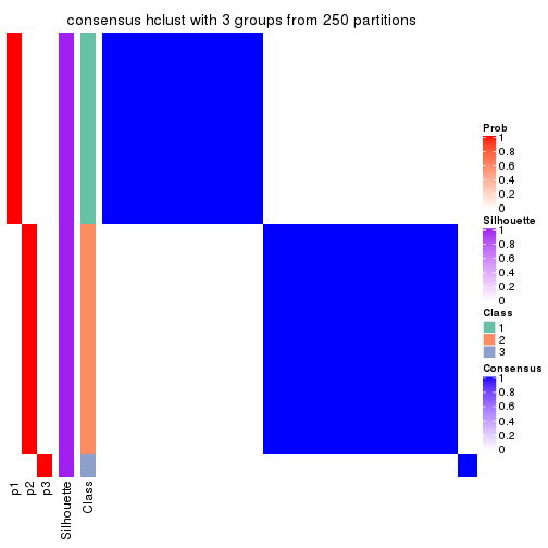
consensus_heatmap(res, k = 4)
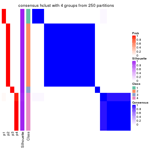
consensus_heatmap(res, k = 5)
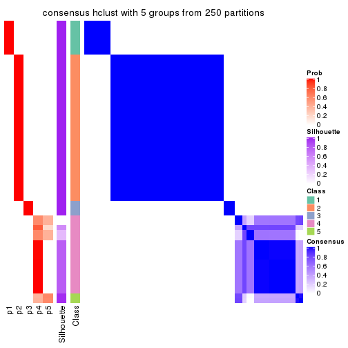
consensus_heatmap(res, k = 6)
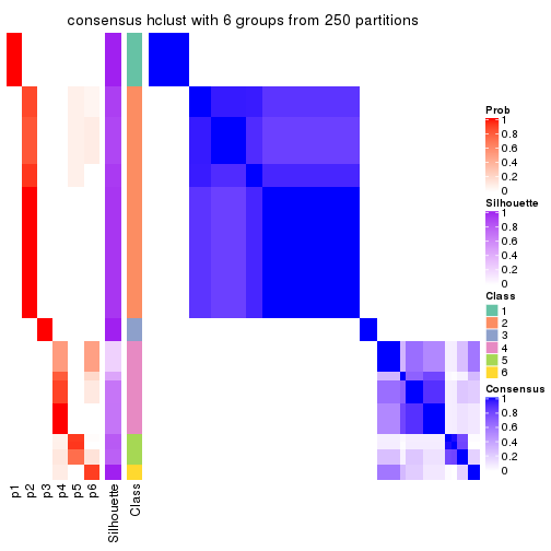
Heatmaps for the membership of samples in all partitions to see how consistent they are:
membership_heatmap(res, k = 2)

membership_heatmap(res, k = 3)

membership_heatmap(res, k = 4)
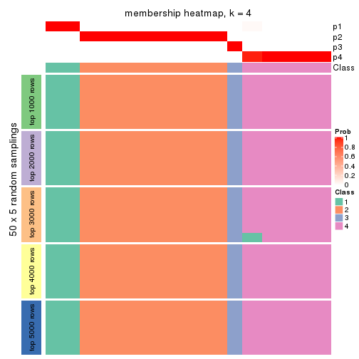
membership_heatmap(res, k = 5)
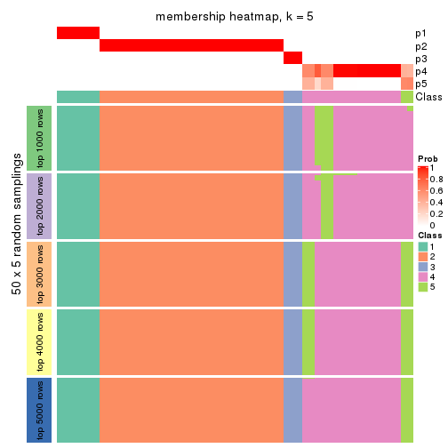
membership_heatmap(res, k = 6)
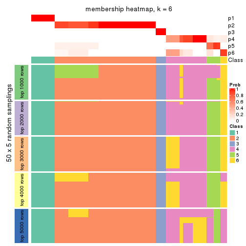
As soon as we have had the classes for columns, we can look for signatures which are significantly different between classes which can be candidate marks for certain classes. Following are the heatmaps for signatures.
Signature heatmaps where rows are scaled:
get_signatures(res, k = 2)

get_signatures(res, k = 3)

get_signatures(res, k = 4)
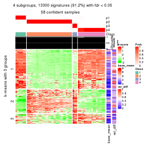
get_signatures(res, k = 5)
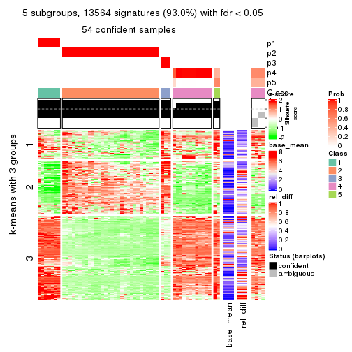
get_signatures(res, k = 6)
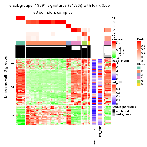
Signature heatmaps where rows are not scaled:
get_signatures(res, k = 2, scale_rows = FALSE)

get_signatures(res, k = 3, scale_rows = FALSE)
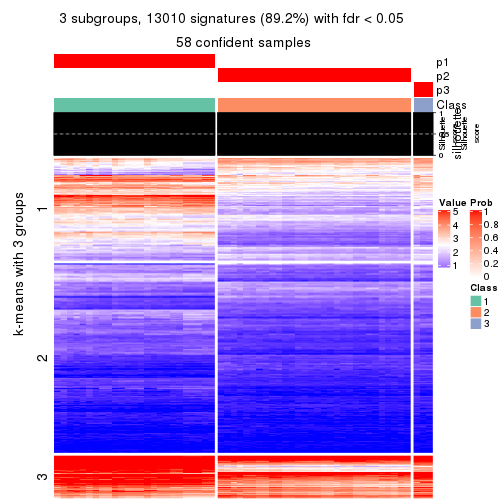
get_signatures(res, k = 4, scale_rows = FALSE)
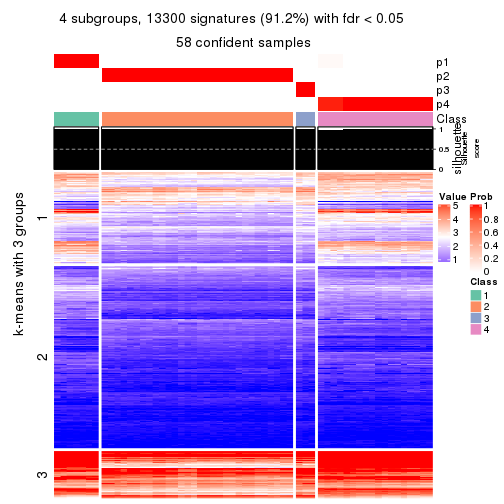
get_signatures(res, k = 5, scale_rows = FALSE)
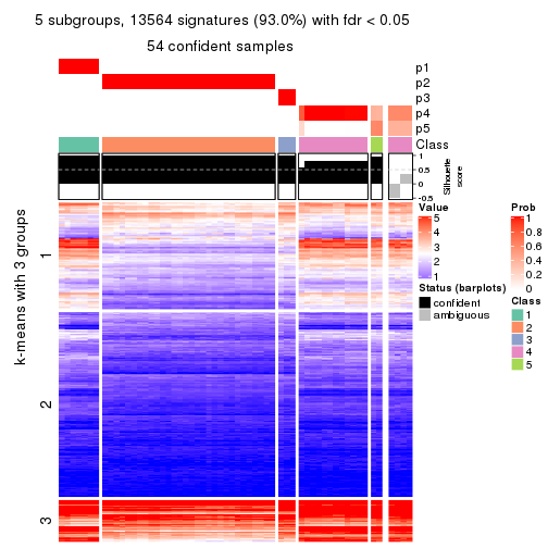
get_signatures(res, k = 6, scale_rows = FALSE)
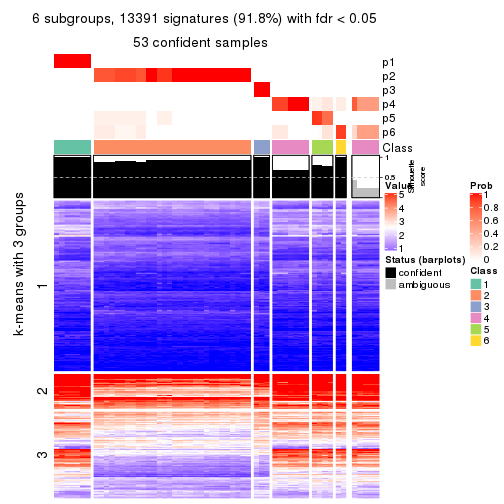
Compare the overlap of signatures from different k:
compare_signatures(res)
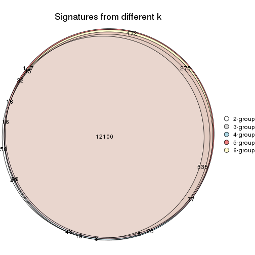
get_signature() returns a data frame invisibly. TO get the list of signatures, the function
call should be assigned to a variable explicitly. In following code, if plot argument is set
to FALSE, no heatmap is plotted while only the differential analysis is performed.
# code only for demonstration
tb = get_signature(res, k = ..., plot = FALSE)
An example of the output of tb is:
#> which_row fdr mean_1 mean_2 scaled_mean_1 scaled_mean_2 km
#> 1 38 0.042760348 8.373488 9.131774 -0.5533452 0.5164555 1
#> 2 40 0.018707592 7.106213 8.469186 -0.6173731 0.5762149 1
#> 3 55 0.019134737 10.221463 11.207825 -0.6159697 0.5749050 1
#> 4 59 0.006059896 5.921854 7.869574 -0.6899429 0.6439467 1
#> 5 60 0.018055526 8.928898 10.211722 -0.6204761 0.5791110 1
#> 6 98 0.009384629 15.714769 14.887706 0.6635654 -0.6193277 2
...
The columns in tb are:
which_row: row indices corresponding to the input matrix.fdr: FDR for the differential test. mean_x: The mean value in group x.scaled_mean_x: The mean value in group x after rows are scaled.km: Row groups if k-means clustering is applied to rows.UMAP plot which shows how samples are separated.
dimension_reduction(res, k = 2, method = "UMAP")

dimension_reduction(res, k = 3, method = "UMAP")
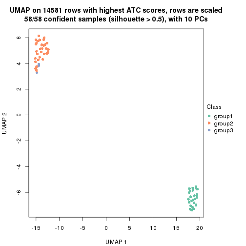
dimension_reduction(res, k = 4, method = "UMAP")

dimension_reduction(res, k = 5, method = "UMAP")
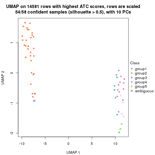
dimension_reduction(res, k = 6, method = "UMAP")
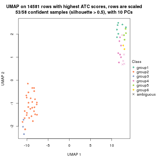
Following heatmap shows how subgroups are split when increasing k:
collect_classes(res)
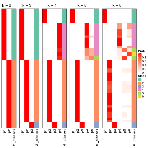
If matrix rows can be associated to genes, consider to use functional_enrichment(res,
...) to perform function enrichment for the signature genes. See this vignette for more detailed explanations.
The object with results only for a single top-value method and a single partition method can be extracted as:
res = res_list["ATC", "kmeans"]
# you can also extract it by
# res = res_list["ATC:kmeans"]
A summary of res and all the functions that can be applied to it:
res
#> A 'ConsensusPartition' object with k = 2, 3, 4, 5, 6.
#> On a matrix with 14581 rows and 58 columns.
#> Top rows (1000, 2000, 3000, 4000, 5000) are extracted by 'ATC' method.
#> Subgroups are detected by 'kmeans' method.
#> Performed in total 1250 partitions by row resampling.
#> Best k for subgroups seems to be 2.
#>
#> Following methods can be applied to this 'ConsensusPartition' object:
#> [1] "cola_report" "collect_classes" "collect_plots"
#> [4] "collect_stats" "colnames" "compare_signatures"
#> [7] "consensus_heatmap" "dimension_reduction" "functional_enrichment"
#> [10] "get_anno_col" "get_anno" "get_classes"
#> [13] "get_consensus" "get_matrix" "get_membership"
#> [16] "get_param" "get_signatures" "get_stats"
#> [19] "is_best_k" "is_stable_k" "membership_heatmap"
#> [22] "ncol" "nrow" "plot_ecdf"
#> [25] "rownames" "select_partition_number" "show"
#> [28] "suggest_best_k" "test_to_known_factors"
collect_plots() function collects all the plots made from res for all k (number of partitions)
into one single page to provide an easy and fast comparison between different k.
collect_plots(res)
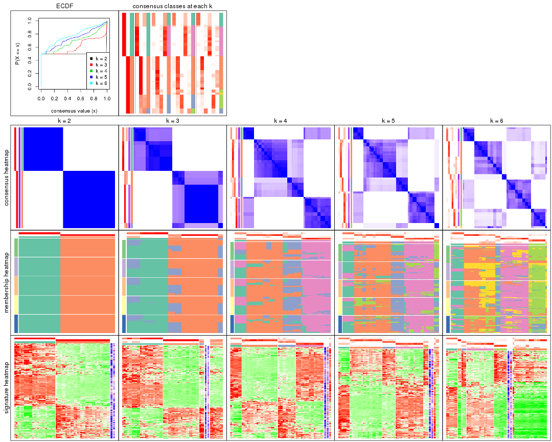
The plots are:
k and the heatmap of
predicted classes for each k.k.k.k.All the plots in panels can be made by individual functions and they are plotted later in this section.
select_partition_number() produces several plots showing different
statistics for choosing “optimized” k. There are following statistics:
k;k, the area increased is defined as \(A_k - A_{k-1}\).The detailed explanations of these statistics can be found in the cola vignette.
Generally speaking, lower PAC score, higher mean silhouette score or higher
concordance corresponds to better partition. Rand index and Jaccard index
measure how similar the current partition is compared to partition with k-1.
If they are too similar, we won't accept k is better than k-1.
select_partition_number(res)
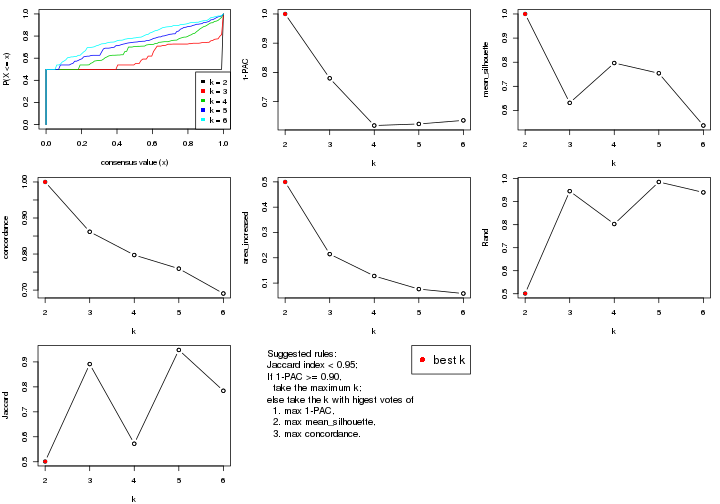
The numeric values for all these statistics can be obtained by get_stats().
get_stats(res)
#> k 1-PAC mean_silhouette concordance area_increased Rand Jaccard
#> 2 2 1.000 1.000 1.000 0.4996 0.501 0.501
#> 3 3 0.780 0.631 0.862 0.2145 0.946 0.891
#> 4 4 0.618 0.797 0.797 0.1281 0.803 0.572
#> 5 5 0.624 0.754 0.760 0.0763 0.985 0.948
#> 6 6 0.636 0.538 0.690 0.0588 0.940 0.784
suggest_best_k() suggests the best \(k\) based on these statistics. The rules are as follows:
suggest_best_k(res)
#> [1] 2
Following shows the table of the partitions (You need to click the show/hide
code output link to see it). The membership matrix (columns with name p*)
is inferred by
clue::cl_consensus()
function with the SE method. Basically the value in the membership matrix
represents the probability to belong to a certain group. The finall class
label for an item is determined with the group with highest probability it
belongs to.
In get_classes() function, the entropy is calculated from the membership
matrix and the silhouette score is calculated from the consensus matrix.
cbind(get_classes(res, k = 2), get_membership(res, k = 2))
#> class entropy silhouette p1 p2
#> ERR789082 2 0 1 0 1
#> ERR789083 2 0 1 0 1
#> ERR789191 2 0 1 0 1
#> ERR789192 2 0 1 0 1
#> ERR789213 1 0 1 1 0
#> ERR789385 1 0 1 1 0
#> ERR789393 1 0 1 1 0
#> ERR789394 1 0 1 1 0
#> ERR789193 2 0 1 0 1
#> ERR789194 2 0 1 0 1
#> ERR789195 2 0 1 0 1
#> ERR789196 2 0 1 0 1
#> ERR789388 1 0 1 1 0
#> ERR789197 2 0 1 0 1
#> ERR789198 2 0 1 0 1
#> ERR789214 1 0 1 1 0
#> ERR789397 1 0 1 1 0
#> ERR789398 1 0 1 1 0
#> ERR789199 2 0 1 0 1
#> ERR789200 2 0 1 0 1
#> ERR789201 2 0 1 0 1
#> ERR789202 2 0 1 0 1
#> ERR789215 1 0 1 1 0
#> ERR789203 2 0 1 0 1
#> ERR789204 2 0 1 0 1
#> ERR789383 1 0 1 1 0
#> ERR789205 2 0 1 0 1
#> ERR789206 2 0 1 0 1
#> ERR789399 1 0 1 1 0
#> ERR789400 1 0 1 1 0
#> ERR789207 2 0 1 0 1
#> ERR789208 2 0 1 0 1
#> ERR789209 2 0 1 0 1
#> ERR789210 2 0 1 0 1
#> ERR789211 2 0 1 0 1
#> ERR789212 2 0 1 0 1
#> ERR789386 1 0 1 1 0
#> ERR789076 2 0 1 0 1
#> ERR789077 2 0 1 0 1
#> ERR789384 1 0 1 1 0
#> ERR789078 2 0 1 0 1
#> ERR789079 2 0 1 0 1
#> ERR789216 1 0 1 1 0
#> ERR789080 2 0 1 0 1
#> ERR789387 1 0 1 1 0
#> ERR789081 2 0 1 0 1
#> ERR789064 2 0 1 0 1
#> ERR779485 2 0 1 0 1
#> ERR789065 2 0 1 0 1
#> ERR789401 1 0 1 1 0
#> ERR789402 1 0 1 1 0
#> ERR789403 1 0 1 1 0
#> ERR789389 1 0 1 1 0
#> ERR789395 1 0 1 1 0
#> ERR789396 1 0 1 1 0
#> ERR789390 1 0 1 1 0
#> ERR789391 1 0 1 1 0
#> ERR789392 1 0 1 1 0
cbind(get_classes(res, k = 3), get_membership(res, k = 3))
#> class entropy silhouette p1 p2 p3
#> ERR789082 2 0.0000 0.777 0.000 1.000 0.000
#> ERR789083 2 0.0000 0.777 0.000 1.000 0.000
#> ERR789191 2 0.0000 0.777 0.000 1.000 0.000
#> ERR789192 2 0.0000 0.777 0.000 1.000 0.000
#> ERR789213 1 0.0747 0.883 0.984 0.000 0.016
#> ERR789385 1 0.0747 0.883 0.984 0.000 0.016
#> ERR789393 1 0.0000 0.885 1.000 0.000 0.000
#> ERR789394 1 0.0000 0.885 1.000 0.000 0.000
#> ERR789193 3 0.6126 1.000 0.000 0.400 0.600
#> ERR789194 3 0.6126 1.000 0.000 0.400 0.600
#> ERR789195 2 0.6140 -0.426 0.000 0.596 0.404
#> ERR789196 2 0.6140 -0.426 0.000 0.596 0.404
#> ERR789388 1 0.0000 0.885 1.000 0.000 0.000
#> ERR789197 2 0.0000 0.777 0.000 1.000 0.000
#> ERR789198 2 0.0000 0.777 0.000 1.000 0.000
#> ERR789214 1 0.0747 0.883 0.984 0.000 0.016
#> ERR789397 1 0.0000 0.885 1.000 0.000 0.000
#> ERR789398 1 0.0000 0.885 1.000 0.000 0.000
#> ERR789199 2 0.0000 0.777 0.000 1.000 0.000
#> ERR789200 2 0.0000 0.777 0.000 1.000 0.000
#> ERR789201 2 0.0000 0.777 0.000 1.000 0.000
#> ERR789202 2 0.0000 0.777 0.000 1.000 0.000
#> ERR789215 1 0.1031 0.881 0.976 0.000 0.024
#> ERR789203 2 0.6295 -0.645 0.000 0.528 0.472
#> ERR789204 2 0.6295 -0.645 0.000 0.528 0.472
#> ERR789383 1 0.6062 0.747 0.616 0.000 0.384
#> ERR789205 2 0.6215 -0.505 0.000 0.572 0.428
#> ERR789206 2 0.6215 -0.505 0.000 0.572 0.428
#> ERR789399 1 0.1964 0.874 0.944 0.000 0.056
#> ERR789400 1 0.1964 0.874 0.944 0.000 0.056
#> ERR789207 2 0.0000 0.777 0.000 1.000 0.000
#> ERR789208 2 0.0000 0.777 0.000 1.000 0.000
#> ERR789209 2 0.0000 0.777 0.000 1.000 0.000
#> ERR789210 2 0.0000 0.777 0.000 1.000 0.000
#> ERR789211 2 0.0000 0.777 0.000 1.000 0.000
#> ERR789212 2 0.0000 0.777 0.000 1.000 0.000
#> ERR789386 1 0.1031 0.881 0.976 0.000 0.024
#> ERR789076 2 0.6280 -0.609 0.000 0.540 0.460
#> ERR789077 2 0.0000 0.777 0.000 1.000 0.000
#> ERR789384 1 0.1031 0.881 0.976 0.000 0.024
#> ERR789078 2 0.0000 0.777 0.000 1.000 0.000
#> ERR789079 2 0.0000 0.777 0.000 1.000 0.000
#> ERR789216 1 0.1031 0.881 0.976 0.000 0.024
#> ERR789080 2 0.0000 0.777 0.000 1.000 0.000
#> ERR789387 1 0.5859 0.773 0.656 0.000 0.344
#> ERR789081 2 0.0000 0.777 0.000 1.000 0.000
#> ERR789064 2 0.0000 0.777 0.000 1.000 0.000
#> ERR779485 3 0.6126 1.000 0.000 0.400 0.600
#> ERR789065 2 0.6309 -0.734 0.000 0.500 0.500
#> ERR789401 1 0.6026 0.750 0.624 0.000 0.376
#> ERR789402 1 0.6026 0.750 0.624 0.000 0.376
#> ERR789403 1 0.6026 0.750 0.624 0.000 0.376
#> ERR789389 1 0.6062 0.747 0.616 0.000 0.384
#> ERR789395 1 0.6026 0.750 0.624 0.000 0.376
#> ERR789396 1 0.6026 0.750 0.624 0.000 0.376
#> ERR789390 1 0.0000 0.885 1.000 0.000 0.000
#> ERR789391 1 0.0000 0.885 1.000 0.000 0.000
#> ERR789392 1 0.0000 0.885 1.000 0.000 0.000
cbind(get_classes(res, k = 4), get_membership(res, k = 4))
#> class entropy silhouette p1 p2 p3 p4
#> ERR789082 2 0.2859 0.855 0.112 0.880 0.008 0.000
#> ERR789083 2 0.2859 0.855 0.112 0.880 0.008 0.000
#> ERR789191 2 0.2976 0.852 0.120 0.872 0.008 0.000
#> ERR789192 2 0.2976 0.852 0.120 0.872 0.008 0.000
#> ERR789213 4 0.3335 0.810 0.020 0.000 0.120 0.860
#> ERR789385 4 0.3219 0.814 0.020 0.000 0.112 0.868
#> ERR789393 4 0.1302 0.816 0.000 0.000 0.044 0.956
#> ERR789394 4 0.1302 0.816 0.000 0.000 0.044 0.956
#> ERR789193 3 0.7114 0.710 0.252 0.188 0.560 0.000
#> ERR789194 3 0.7114 0.710 0.252 0.188 0.560 0.000
#> ERR789195 3 0.4585 0.792 0.000 0.332 0.668 0.000
#> ERR789196 3 0.4585 0.792 0.000 0.332 0.668 0.000
#> ERR789388 4 0.2125 0.824 0.004 0.000 0.076 0.920
#> ERR789197 2 0.3325 0.853 0.112 0.864 0.024 0.000
#> ERR789198 2 0.3325 0.853 0.112 0.864 0.024 0.000
#> ERR789214 4 0.3037 0.817 0.020 0.000 0.100 0.880
#> ERR789397 4 0.0921 0.819 0.000 0.000 0.028 0.972
#> ERR789398 4 0.0921 0.819 0.000 0.000 0.028 0.972
#> ERR789199 2 0.2976 0.852 0.120 0.872 0.008 0.000
#> ERR789200 2 0.2976 0.852 0.120 0.872 0.008 0.000
#> ERR789201 2 0.4567 0.535 0.016 0.740 0.244 0.000
#> ERR789202 2 0.4567 0.535 0.016 0.740 0.244 0.000
#> ERR789215 4 0.3441 0.792 0.024 0.000 0.120 0.856
#> ERR789203 3 0.4690 0.835 0.016 0.260 0.724 0.000
#> ERR789204 3 0.4690 0.835 0.016 0.260 0.724 0.000
#> ERR789383 1 0.5388 0.980 0.532 0.000 0.012 0.456
#> ERR789205 3 0.4564 0.801 0.000 0.328 0.672 0.000
#> ERR789206 3 0.4564 0.801 0.000 0.328 0.672 0.000
#> ERR789399 4 0.2924 0.673 0.100 0.000 0.016 0.884
#> ERR789400 4 0.2924 0.673 0.100 0.000 0.016 0.884
#> ERR789207 2 0.0336 0.850 0.008 0.992 0.000 0.000
#> ERR789208 2 0.0336 0.850 0.008 0.992 0.000 0.000
#> ERR789209 2 0.2760 0.751 0.000 0.872 0.128 0.000
#> ERR789210 2 0.2760 0.751 0.000 0.872 0.128 0.000
#> ERR789211 2 0.0592 0.849 0.000 0.984 0.016 0.000
#> ERR789212 2 0.0592 0.849 0.000 0.984 0.016 0.000
#> ERR789386 4 0.3441 0.791 0.024 0.000 0.120 0.856
#> ERR789076 3 0.4539 0.830 0.008 0.272 0.720 0.000
#> ERR789077 2 0.2944 0.851 0.128 0.868 0.004 0.000
#> ERR789384 4 0.3441 0.791 0.024 0.000 0.120 0.856
#> ERR789078 2 0.1004 0.845 0.024 0.972 0.004 0.000
#> ERR789079 2 0.1902 0.827 0.064 0.932 0.004 0.000
#> ERR789216 4 0.3441 0.791 0.024 0.000 0.120 0.856
#> ERR789080 2 0.4071 0.727 0.064 0.832 0.104 0.000
#> ERR789387 4 0.6668 -0.576 0.380 0.000 0.092 0.528
#> ERR789081 2 0.1902 0.827 0.064 0.932 0.004 0.000
#> ERR789064 2 0.2345 0.858 0.100 0.900 0.000 0.000
#> ERR779485 3 0.7114 0.710 0.252 0.188 0.560 0.000
#> ERR789065 3 0.4776 0.829 0.024 0.244 0.732 0.000
#> ERR789401 1 0.4977 0.990 0.540 0.000 0.000 0.460
#> ERR789402 1 0.5147 0.990 0.536 0.000 0.004 0.460
#> ERR789403 1 0.4977 0.990 0.540 0.000 0.000 0.460
#> ERR789389 1 0.5388 0.980 0.532 0.000 0.012 0.456
#> ERR789395 1 0.5147 0.990 0.536 0.000 0.004 0.460
#> ERR789396 1 0.5147 0.990 0.536 0.000 0.004 0.460
#> ERR789390 4 0.0657 0.815 0.004 0.000 0.012 0.984
#> ERR789391 4 0.0657 0.815 0.004 0.000 0.012 0.984
#> ERR789392 4 0.1302 0.816 0.000 0.000 0.044 0.956
cbind(get_classes(res, k = 5), get_membership(res, k = 5))
#> class entropy silhouette p1 p2 p3 p4 p5
#> ERR789082 2 0.236 0.763 0.104 0.888 0.000 0.000 0.008
#> ERR789083 2 0.236 0.763 0.104 0.888 0.000 0.000 0.008
#> ERR789191 2 0.306 0.757 0.128 0.848 0.000 0.000 0.024
#> ERR789192 2 0.306 0.757 0.128 0.848 0.000 0.000 0.024
#> ERR789213 4 0.289 0.751 0.000 0.000 0.000 0.824 0.176
#> ERR789385 4 0.273 0.757 0.000 0.000 0.000 0.840 0.160
#> ERR789393 4 0.372 0.761 0.012 0.000 0.000 0.760 0.228
#> ERR789394 4 0.372 0.761 0.012 0.000 0.000 0.760 0.228
#> ERR789193 5 0.566 0.998 0.000 0.080 0.408 0.000 0.512
#> ERR789194 5 0.566 0.998 0.000 0.080 0.408 0.000 0.512
#> ERR789195 3 0.349 0.901 0.008 0.212 0.780 0.000 0.000
#> ERR789196 3 0.349 0.901 0.008 0.212 0.780 0.000 0.000
#> ERR789388 4 0.146 0.788 0.008 0.000 0.008 0.952 0.032
#> ERR789197 2 0.296 0.758 0.112 0.864 0.016 0.000 0.008
#> ERR789198 2 0.296 0.758 0.112 0.864 0.016 0.000 0.008
#> ERR789214 4 0.236 0.782 0.000 0.000 0.024 0.900 0.076
#> ERR789397 4 0.291 0.786 0.012 0.000 0.008 0.864 0.116
#> ERR789398 4 0.291 0.786 0.012 0.000 0.008 0.864 0.116
#> ERR789199 2 0.287 0.756 0.128 0.856 0.000 0.000 0.016
#> ERR789200 2 0.287 0.756 0.128 0.856 0.000 0.000 0.016
#> ERR789201 2 0.574 -0.046 0.004 0.476 0.448 0.000 0.072
#> ERR789202 2 0.574 -0.046 0.004 0.476 0.448 0.000 0.072
#> ERR789215 4 0.242 0.760 0.000 0.000 0.024 0.896 0.080
#> ERR789203 3 0.350 0.884 0.008 0.160 0.816 0.000 0.016
#> ERR789204 3 0.350 0.884 0.008 0.160 0.816 0.000 0.016
#> ERR789383 1 0.477 0.954 0.660 0.000 0.012 0.308 0.020
#> ERR789205 3 0.330 0.906 0.000 0.204 0.792 0.000 0.004
#> ERR789206 3 0.330 0.906 0.000 0.204 0.792 0.000 0.004
#> ERR789399 4 0.400 0.733 0.076 0.000 0.004 0.804 0.116
#> ERR789400 4 0.400 0.733 0.076 0.000 0.004 0.804 0.116
#> ERR789207 2 0.305 0.753 0.064 0.864 0.000 0.000 0.072
#> ERR789208 2 0.305 0.753 0.064 0.864 0.000 0.000 0.072
#> ERR789209 2 0.468 0.575 0.004 0.720 0.220 0.000 0.056
#> ERR789210 2 0.468 0.575 0.004 0.720 0.220 0.000 0.056
#> ERR789211 2 0.297 0.753 0.020 0.884 0.040 0.000 0.056
#> ERR789212 2 0.297 0.753 0.020 0.884 0.040 0.000 0.056
#> ERR789386 4 0.287 0.757 0.000 0.000 0.040 0.872 0.088
#> ERR789076 3 0.301 0.894 0.008 0.160 0.832 0.000 0.000
#> ERR789077 2 0.380 0.742 0.128 0.820 0.016 0.000 0.036
#> ERR789384 4 0.287 0.757 0.000 0.000 0.040 0.872 0.088
#> ERR789078 2 0.440 0.727 0.108 0.788 0.016 0.000 0.088
#> ERR789079 2 0.521 0.682 0.160 0.716 0.016 0.000 0.108
#> ERR789216 4 0.287 0.757 0.000 0.000 0.040 0.872 0.088
#> ERR789080 2 0.641 0.608 0.160 0.644 0.088 0.000 0.108
#> ERR789387 4 0.674 -0.421 0.368 0.000 0.052 0.492 0.088
#> ERR789081 2 0.521 0.682 0.160 0.716 0.016 0.000 0.108
#> ERR789064 2 0.207 0.767 0.092 0.904 0.000 0.000 0.004
#> ERR779485 5 0.580 0.997 0.004 0.080 0.408 0.000 0.508
#> ERR789065 3 0.320 0.828 0.008 0.132 0.844 0.000 0.016
#> ERR789401 1 0.399 0.965 0.688 0.000 0.004 0.308 0.000
#> ERR789402 1 0.504 0.961 0.648 0.000 0.024 0.308 0.020
#> ERR789403 1 0.399 0.965 0.688 0.000 0.004 0.308 0.000
#> ERR789389 1 0.477 0.954 0.660 0.000 0.012 0.308 0.020
#> ERR789395 1 0.504 0.961 0.648 0.000 0.024 0.308 0.020
#> ERR789396 1 0.504 0.961 0.648 0.000 0.024 0.308 0.020
#> ERR789390 4 0.280 0.784 0.016 0.000 0.012 0.880 0.092
#> ERR789391 4 0.280 0.784 0.016 0.000 0.012 0.880 0.092
#> ERR789392 4 0.372 0.761 0.012 0.000 0.000 0.760 0.228
cbind(get_classes(res, k = 6), get_membership(res, k = 6))
#> class entropy silhouette p1 p2 p3 p4 p5 p6
#> ERR789082 2 0.0748 0.5008 0.016 0.976 0.000 0.000 0.004 0.004
#> ERR789083 2 0.0748 0.5008 0.016 0.976 0.000 0.000 0.004 0.004
#> ERR789191 2 0.1585 0.4847 0.036 0.940 0.012 0.000 0.000 0.012
#> ERR789192 2 0.1585 0.4847 0.036 0.940 0.012 0.000 0.000 0.012
#> ERR789213 4 0.5497 0.6855 0.004 0.000 0.076 0.584 0.024 0.312
#> ERR789385 4 0.4987 0.6908 0.004 0.000 0.068 0.608 0.004 0.316
#> ERR789393 4 0.3915 0.7039 0.004 0.000 0.052 0.756 0.000 0.188
#> ERR789394 4 0.3915 0.7039 0.004 0.000 0.052 0.756 0.000 0.188
#> ERR789193 3 0.4382 0.9877 0.000 0.060 0.676 0.000 0.264 0.000
#> ERR789194 3 0.4382 0.9877 0.000 0.060 0.676 0.000 0.264 0.000
#> ERR789195 5 0.3294 0.8003 0.032 0.128 0.004 0.000 0.828 0.008
#> ERR789196 5 0.3294 0.8003 0.032 0.128 0.004 0.000 0.828 0.008
#> ERR789388 4 0.3665 0.7316 0.000 0.000 0.052 0.800 0.012 0.136
#> ERR789197 2 0.2118 0.4840 0.016 0.920 0.008 0.000 0.036 0.020
#> ERR789198 2 0.2118 0.4840 0.016 0.920 0.008 0.000 0.036 0.020
#> ERR789214 4 0.5317 0.7216 0.004 0.000 0.092 0.668 0.036 0.200
#> ERR789397 4 0.1629 0.7396 0.004 0.000 0.024 0.940 0.004 0.028
#> ERR789398 4 0.1629 0.7396 0.004 0.000 0.024 0.940 0.004 0.028
#> ERR789199 2 0.1666 0.4882 0.036 0.936 0.020 0.000 0.000 0.008
#> ERR789200 2 0.1666 0.4882 0.036 0.936 0.020 0.000 0.000 0.008
#> ERR789201 5 0.5610 0.4115 0.008 0.260 0.008 0.000 0.592 0.132
#> ERR789202 5 0.5610 0.4115 0.008 0.260 0.008 0.000 0.592 0.132
#> ERR789215 4 0.5593 0.6808 0.016 0.000 0.124 0.660 0.028 0.172
#> ERR789203 5 0.3069 0.7722 0.012 0.088 0.028 0.000 0.860 0.012
#> ERR789204 5 0.3069 0.7722 0.012 0.088 0.028 0.000 0.860 0.012
#> ERR789383 1 0.4356 0.8766 0.728 0.000 0.040 0.212 0.008 0.012
#> ERR789205 5 0.2146 0.8062 0.004 0.116 0.000 0.000 0.880 0.000
#> ERR789206 5 0.2146 0.8062 0.004 0.116 0.000 0.000 0.880 0.000
#> ERR789399 4 0.2932 0.6731 0.080 0.000 0.028 0.868 0.004 0.020
#> ERR789400 4 0.2932 0.6731 0.080 0.000 0.028 0.868 0.004 0.020
#> ERR789207 2 0.4084 0.0348 0.000 0.588 0.000 0.000 0.012 0.400
#> ERR789208 2 0.4084 0.0348 0.000 0.588 0.000 0.000 0.012 0.400
#> ERR789209 2 0.6090 -0.0946 0.004 0.436 0.000 0.000 0.240 0.320
#> ERR789210 2 0.6090 -0.0946 0.004 0.436 0.000 0.000 0.240 0.320
#> ERR789211 2 0.4818 0.1212 0.004 0.588 0.000 0.000 0.056 0.352
#> ERR789212 2 0.4818 0.1212 0.004 0.588 0.000 0.000 0.056 0.352
#> ERR789386 4 0.5668 0.6657 0.016 0.000 0.176 0.620 0.008 0.180
#> ERR789076 5 0.3161 0.7906 0.040 0.092 0.000 0.000 0.848 0.020
#> ERR789077 2 0.4586 -0.0823 0.076 0.660 0.000 0.000 0.000 0.264
#> ERR789384 4 0.5590 0.6667 0.016 0.000 0.172 0.620 0.004 0.188
#> ERR789078 2 0.5050 -0.3393 0.076 0.572 0.004 0.000 0.000 0.348
#> ERR789079 2 0.5676 -0.7313 0.092 0.452 0.008 0.000 0.008 0.440
#> ERR789216 4 0.5619 0.6652 0.016 0.000 0.184 0.616 0.004 0.180
#> ERR789080 6 0.6561 0.0000 0.092 0.384 0.008 0.000 0.072 0.444
#> ERR789387 1 0.7528 0.3011 0.364 0.000 0.196 0.324 0.016 0.100
#> ERR789081 2 0.5676 -0.7313 0.092 0.452 0.008 0.000 0.008 0.440
#> ERR789064 2 0.0951 0.4976 0.008 0.968 0.000 0.000 0.004 0.020
#> ERR779485 3 0.4979 0.9755 0.020 0.060 0.660 0.000 0.256 0.004
#> ERR789065 5 0.3557 0.7422 0.040 0.076 0.028 0.000 0.840 0.016
#> ERR789401 1 0.3109 0.8980 0.772 0.000 0.000 0.224 0.004 0.000
#> ERR789402 1 0.3810 0.8974 0.748 0.000 0.008 0.224 0.012 0.008
#> ERR789403 1 0.3109 0.8980 0.772 0.000 0.000 0.224 0.004 0.000
#> ERR789389 1 0.4356 0.8766 0.728 0.000 0.040 0.212 0.008 0.012
#> ERR789395 1 0.3810 0.8974 0.748 0.000 0.008 0.224 0.012 0.008
#> ERR789396 1 0.3810 0.8974 0.748 0.000 0.008 0.224 0.012 0.008
#> ERR789390 4 0.0798 0.7370 0.004 0.000 0.004 0.976 0.012 0.004
#> ERR789391 4 0.0798 0.7370 0.004 0.000 0.004 0.976 0.012 0.004
#> ERR789392 4 0.3915 0.7039 0.004 0.000 0.052 0.756 0.000 0.188
Heatmaps for the consensus matrix. It visualizes the probability of two samples to be in a same group.
consensus_heatmap(res, k = 2)

consensus_heatmap(res, k = 3)
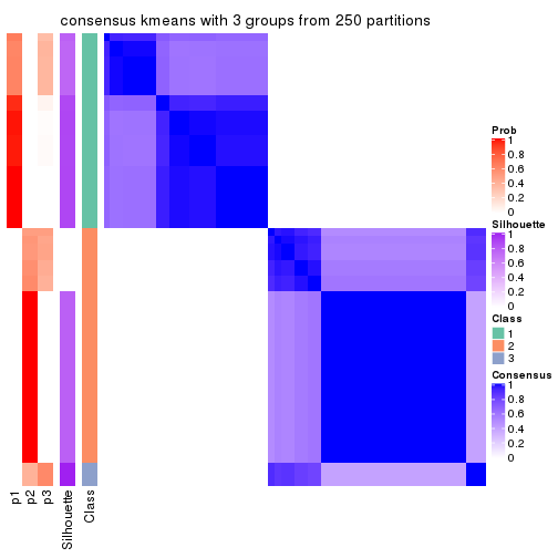
consensus_heatmap(res, k = 4)
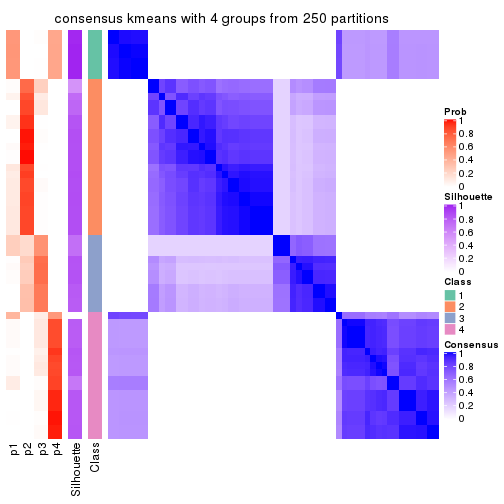
consensus_heatmap(res, k = 5)
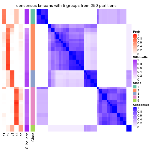
consensus_heatmap(res, k = 6)
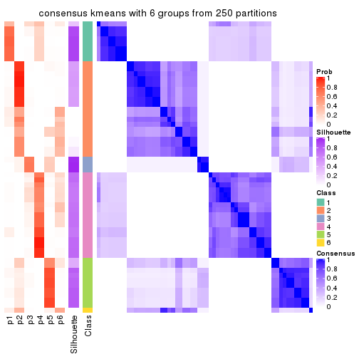
Heatmaps for the membership of samples in all partitions to see how consistent they are:
membership_heatmap(res, k = 2)

membership_heatmap(res, k = 3)
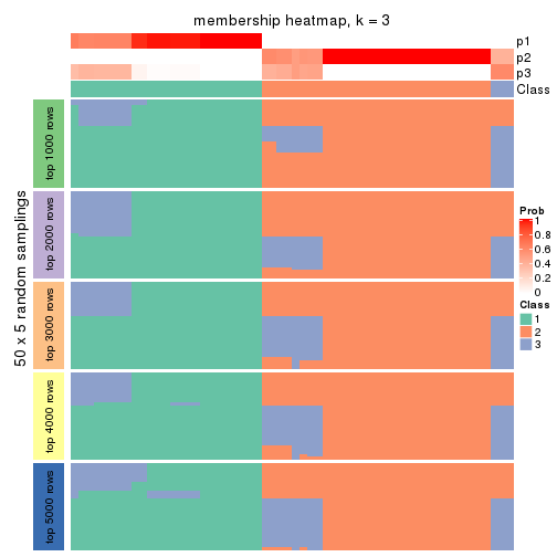
membership_heatmap(res, k = 4)
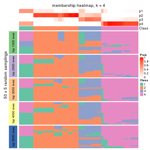
membership_heatmap(res, k = 5)
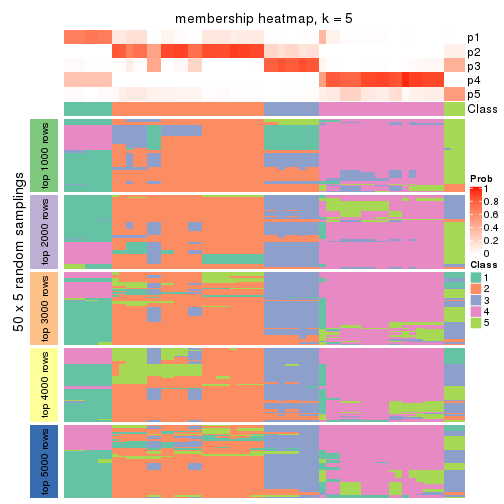
membership_heatmap(res, k = 6)
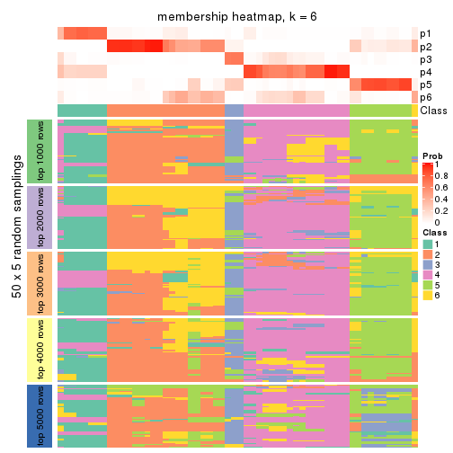
As soon as we have had the classes for columns, we can look for signatures which are significantly different between classes which can be candidate marks for certain classes. Following are the heatmaps for signatures.
Signature heatmaps where rows are scaled:
get_signatures(res, k = 2)

get_signatures(res, k = 3)
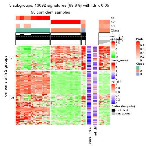
get_signatures(res, k = 4)
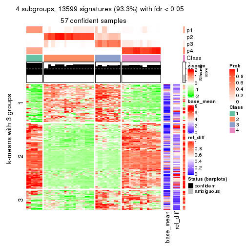
get_signatures(res, k = 5)
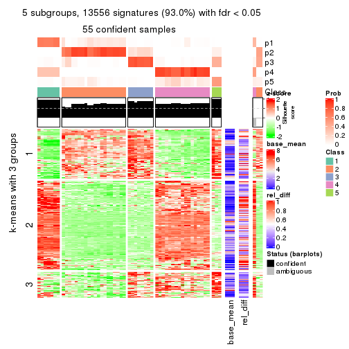
get_signatures(res, k = 6)
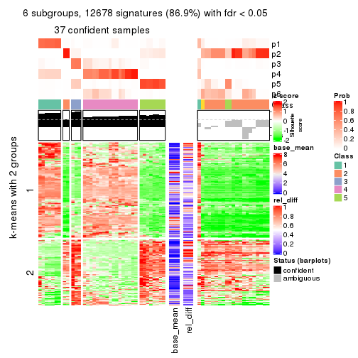
Signature heatmaps where rows are not scaled:
get_signatures(res, k = 2, scale_rows = FALSE)

get_signatures(res, k = 3, scale_rows = FALSE)
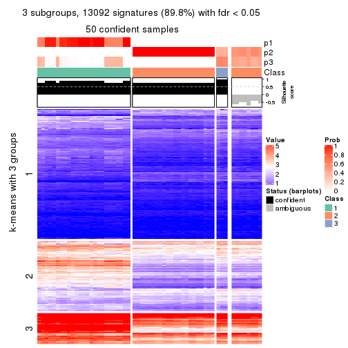
get_signatures(res, k = 4, scale_rows = FALSE)
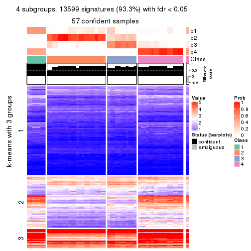
get_signatures(res, k = 5, scale_rows = FALSE)
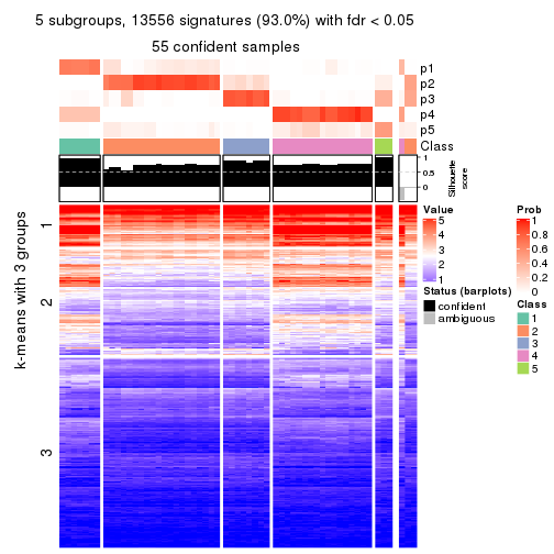
get_signatures(res, k = 6, scale_rows = FALSE)
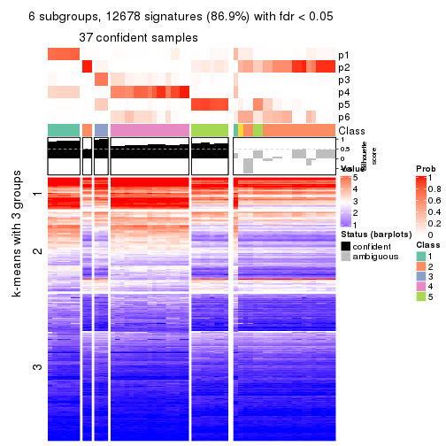
Compare the overlap of signatures from different k:
compare_signatures(res)
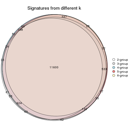
get_signature() returns a data frame invisibly. TO get the list of signatures, the function
call should be assigned to a variable explicitly. In following code, if plot argument is set
to FALSE, no heatmap is plotted while only the differential analysis is performed.
# code only for demonstration
tb = get_signature(res, k = ..., plot = FALSE)
An example of the output of tb is:
#> which_row fdr mean_1 mean_2 scaled_mean_1 scaled_mean_2 km
#> 1 38 0.042760348 8.373488 9.131774 -0.5533452 0.5164555 1
#> 2 40 0.018707592 7.106213 8.469186 -0.6173731 0.5762149 1
#> 3 55 0.019134737 10.221463 11.207825 -0.6159697 0.5749050 1
#> 4 59 0.006059896 5.921854 7.869574 -0.6899429 0.6439467 1
#> 5 60 0.018055526 8.928898 10.211722 -0.6204761 0.5791110 1
#> 6 98 0.009384629 15.714769 14.887706 0.6635654 -0.6193277 2
...
The columns in tb are:
which_row: row indices corresponding to the input matrix.fdr: FDR for the differential test. mean_x: The mean value in group x.scaled_mean_x: The mean value in group x after rows are scaled.km: Row groups if k-means clustering is applied to rows.UMAP plot which shows how samples are separated.
dimension_reduction(res, k = 2, method = "UMAP")

dimension_reduction(res, k = 3, method = "UMAP")
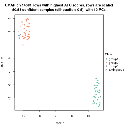
dimension_reduction(res, k = 4, method = "UMAP")
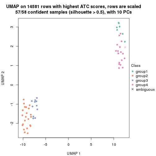
dimension_reduction(res, k = 5, method = "UMAP")
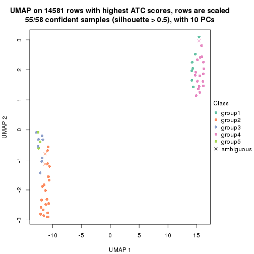
dimension_reduction(res, k = 6, method = "UMAP")
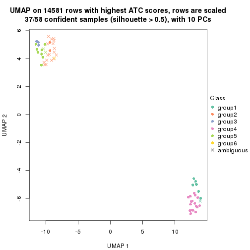
Following heatmap shows how subgroups are split when increasing k:
collect_classes(res)
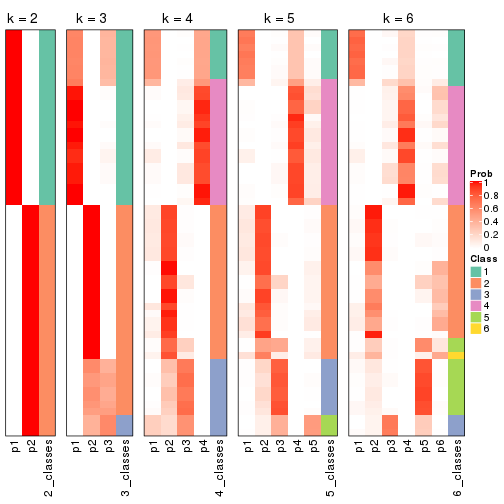
If matrix rows can be associated to genes, consider to use functional_enrichment(res,
...) to perform function enrichment for the signature genes. See this vignette for more detailed explanations.
The object with results only for a single top-value method and a single partition method can be extracted as:
res = res_list["ATC", "skmeans"]
# you can also extract it by
# res = res_list["ATC:skmeans"]
A summary of res and all the functions that can be applied to it:
res
#> A 'ConsensusPartition' object with k = 2, 3, 4, 5, 6.
#> On a matrix with 14581 rows and 58 columns.
#> Top rows (1000, 2000, 3000, 4000, 5000) are extracted by 'ATC' method.
#> Subgroups are detected by 'skmeans' method.
#> Performed in total 1250 partitions by row resampling.
#> Best k for subgroups seems to be 3.
#>
#> Following methods can be applied to this 'ConsensusPartition' object:
#> [1] "cola_report" "collect_classes" "collect_plots"
#> [4] "collect_stats" "colnames" "compare_signatures"
#> [7] "consensus_heatmap" "dimension_reduction" "functional_enrichment"
#> [10] "get_anno_col" "get_anno" "get_classes"
#> [13] "get_consensus" "get_matrix" "get_membership"
#> [16] "get_param" "get_signatures" "get_stats"
#> [19] "is_best_k" "is_stable_k" "membership_heatmap"
#> [22] "ncol" "nrow" "plot_ecdf"
#> [25] "rownames" "select_partition_number" "show"
#> [28] "suggest_best_k" "test_to_known_factors"
collect_plots() function collects all the plots made from res for all k (number of partitions)
into one single page to provide an easy and fast comparison between different k.
collect_plots(res)
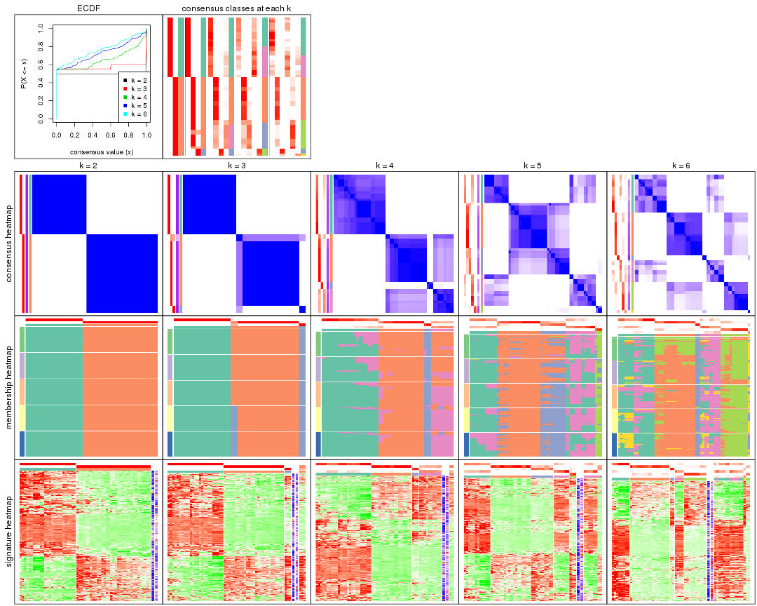
The plots are:
k and the heatmap of
predicted classes for each k.k.k.k.All the plots in panels can be made by individual functions and they are plotted later in this section.
select_partition_number() produces several plots showing different
statistics for choosing “optimized” k. There are following statistics:
k;k, the area increased is defined as \(A_k - A_{k-1}\).The detailed explanations of these statistics can be found in the cola vignette.
Generally speaking, lower PAC score, higher mean silhouette score or higher
concordance corresponds to better partition. Rand index and Jaccard index
measure how similar the current partition is compared to partition with k-1.
If they are too similar, we won't accept k is better than k-1.
select_partition_number(res)
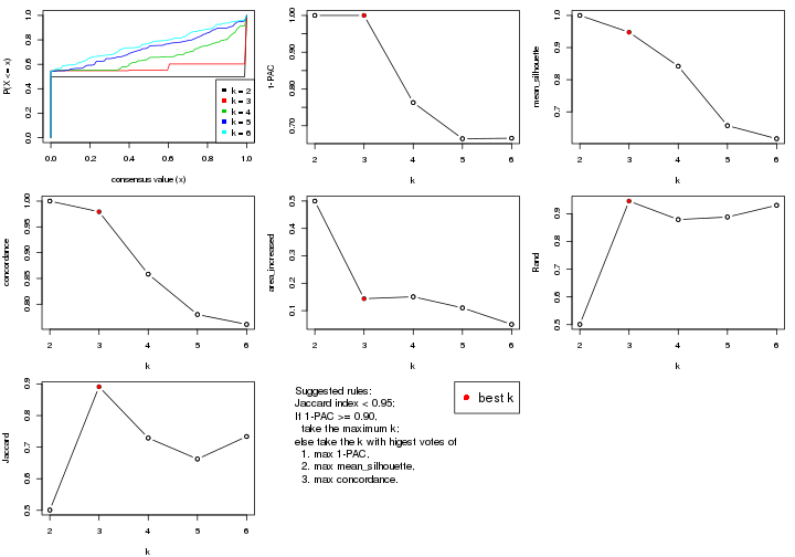
The numeric values for all these statistics can be obtained by get_stats().
get_stats(res)
#> k 1-PAC mean_silhouette concordance area_increased Rand Jaccard
#> 2 2 1.000 1.000 1.000 0.4996 0.501 0.501
#> 3 3 1.000 0.948 0.979 0.1437 0.946 0.891
#> 4 4 0.763 0.842 0.858 0.1506 0.879 0.729
#> 5 5 0.665 0.657 0.780 0.1102 0.888 0.662
#> 6 6 0.666 0.616 0.761 0.0499 0.930 0.734
suggest_best_k() suggests the best \(k\) based on these statistics. The rules are as follows:
suggest_best_k(res)
#> [1] 3
#> attr(,"optional")
#> [1] 2
There is also optional best \(k\) = 2 that is worth to check.
Following shows the table of the partitions (You need to click the show/hide
code output link to see it). The membership matrix (columns with name p*)
is inferred by
clue::cl_consensus()
function with the SE method. Basically the value in the membership matrix
represents the probability to belong to a certain group. The finall class
label for an item is determined with the group with highest probability it
belongs to.
In get_classes() function, the entropy is calculated from the membership
matrix and the silhouette score is calculated from the consensus matrix.
cbind(get_classes(res, k = 2), get_membership(res, k = 2))
#> class entropy silhouette p1 p2
#> ERR789082 2 0 1 0 1
#> ERR789083 2 0 1 0 1
#> ERR789191 2 0 1 0 1
#> ERR789192 2 0 1 0 1
#> ERR789213 1 0 1 1 0
#> ERR789385 1 0 1 1 0
#> ERR789393 1 0 1 1 0
#> ERR789394 1 0 1 1 0
#> ERR789193 2 0 1 0 1
#> ERR789194 2 0 1 0 1
#> ERR789195 2 0 1 0 1
#> ERR789196 2 0 1 0 1
#> ERR789388 1 0 1 1 0
#> ERR789197 2 0 1 0 1
#> ERR789198 2 0 1 0 1
#> ERR789214 1 0 1 1 0
#> ERR789397 1 0 1 1 0
#> ERR789398 1 0 1 1 0
#> ERR789199 2 0 1 0 1
#> ERR789200 2 0 1 0 1
#> ERR789201 2 0 1 0 1
#> ERR789202 2 0 1 0 1
#> ERR789215 1 0 1 1 0
#> ERR789203 2 0 1 0 1
#> ERR789204 2 0 1 0 1
#> ERR789383 1 0 1 1 0
#> ERR789205 2 0 1 0 1
#> ERR789206 2 0 1 0 1
#> ERR789399 1 0 1 1 0
#> ERR789400 1 0 1 1 0
#> ERR789207 2 0 1 0 1
#> ERR789208 2 0 1 0 1
#> ERR789209 2 0 1 0 1
#> ERR789210 2 0 1 0 1
#> ERR789211 2 0 1 0 1
#> ERR789212 2 0 1 0 1
#> ERR789386 1 0 1 1 0
#> ERR789076 2 0 1 0 1
#> ERR789077 2 0 1 0 1
#> ERR789384 1 0 1 1 0
#> ERR789078 2 0 1 0 1
#> ERR789079 2 0 1 0 1
#> ERR789216 1 0 1 1 0
#> ERR789080 2 0 1 0 1
#> ERR789387 1 0 1 1 0
#> ERR789081 2 0 1 0 1
#> ERR789064 2 0 1 0 1
#> ERR779485 2 0 1 0 1
#> ERR789065 2 0 1 0 1
#> ERR789401 1 0 1 1 0
#> ERR789402 1 0 1 1 0
#> ERR789403 1 0 1 1 0
#> ERR789389 1 0 1 1 0
#> ERR789395 1 0 1 1 0
#> ERR789396 1 0 1 1 0
#> ERR789390 1 0 1 1 0
#> ERR789391 1 0 1 1 0
#> ERR789392 1 0 1 1 0
cbind(get_classes(res, k = 3), get_membership(res, k = 3))
#> class entropy silhouette p1 p2 p3
#> ERR789082 2 0.000 0.957 0 1.0 0.0
#> ERR789083 2 0.000 0.957 0 1.0 0.0
#> ERR789191 2 0.000 0.957 0 1.0 0.0
#> ERR789192 2 0.000 0.957 0 1.0 0.0
#> ERR789213 1 0.000 1.000 1 0.0 0.0
#> ERR789385 1 0.000 1.000 1 0.0 0.0
#> ERR789393 1 0.000 1.000 1 0.0 0.0
#> ERR789394 1 0.000 1.000 1 0.0 0.0
#> ERR789193 3 0.000 1.000 0 0.0 1.0
#> ERR789194 3 0.000 1.000 0 0.0 1.0
#> ERR789195 2 0.000 0.957 0 1.0 0.0
#> ERR789196 2 0.000 0.957 0 1.0 0.0
#> ERR789388 1 0.000 1.000 1 0.0 0.0
#> ERR789197 2 0.000 0.957 0 1.0 0.0
#> ERR789198 2 0.000 0.957 0 1.0 0.0
#> ERR789214 1 0.000 1.000 1 0.0 0.0
#> ERR789397 1 0.000 1.000 1 0.0 0.0
#> ERR789398 1 0.000 1.000 1 0.0 0.0
#> ERR789199 2 0.000 0.957 0 1.0 0.0
#> ERR789200 2 0.000 0.957 0 1.0 0.0
#> ERR789201 2 0.000 0.957 0 1.0 0.0
#> ERR789202 2 0.000 0.957 0 1.0 0.0
#> ERR789215 1 0.000 1.000 1 0.0 0.0
#> ERR789203 2 0.613 0.379 0 0.6 0.4
#> ERR789204 2 0.613 0.379 0 0.6 0.4
#> ERR789383 1 0.000 1.000 1 0.0 0.0
#> ERR789205 2 0.000 0.957 0 1.0 0.0
#> ERR789206 2 0.000 0.957 0 1.0 0.0
#> ERR789399 1 0.000 1.000 1 0.0 0.0
#> ERR789400 1 0.000 1.000 1 0.0 0.0
#> ERR789207 2 0.000 0.957 0 1.0 0.0
#> ERR789208 2 0.000 0.957 0 1.0 0.0
#> ERR789209 2 0.000 0.957 0 1.0 0.0
#> ERR789210 2 0.000 0.957 0 1.0 0.0
#> ERR789211 2 0.000 0.957 0 1.0 0.0
#> ERR789212 2 0.000 0.957 0 1.0 0.0
#> ERR789386 1 0.000 1.000 1 0.0 0.0
#> ERR789076 2 0.000 0.957 0 1.0 0.0
#> ERR789077 2 0.000 0.957 0 1.0 0.0
#> ERR789384 1 0.000 1.000 1 0.0 0.0
#> ERR789078 2 0.000 0.957 0 1.0 0.0
#> ERR789079 2 0.000 0.957 0 1.0 0.0
#> ERR789216 1 0.000 1.000 1 0.0 0.0
#> ERR789080 2 0.000 0.957 0 1.0 0.0
#> ERR789387 1 0.000 1.000 1 0.0 0.0
#> ERR789081 2 0.000 0.957 0 1.0 0.0
#> ERR789064 2 0.000 0.957 0 1.0 0.0
#> ERR779485 3 0.000 1.000 0 0.0 1.0
#> ERR789065 2 0.613 0.379 0 0.6 0.4
#> ERR789401 1 0.000 1.000 1 0.0 0.0
#> ERR789402 1 0.000 1.000 1 0.0 0.0
#> ERR789403 1 0.000 1.000 1 0.0 0.0
#> ERR789389 1 0.000 1.000 1 0.0 0.0
#> ERR789395 1 0.000 1.000 1 0.0 0.0
#> ERR789396 1 0.000 1.000 1 0.0 0.0
#> ERR789390 1 0.000 1.000 1 0.0 0.0
#> ERR789391 1 0.000 1.000 1 0.0 0.0
#> ERR789392 1 0.000 1.000 1 0.0 0.0
cbind(get_classes(res, k = 4), get_membership(res, k = 4))
#> class entropy silhouette p1 p2 p3 p4
#> ERR789082 2 0.0000 0.901 0.000 1.000 0.000 0.000
#> ERR789083 2 0.0000 0.901 0.000 1.000 0.000 0.000
#> ERR789191 2 0.0000 0.901 0.000 1.000 0.000 0.000
#> ERR789192 2 0.0000 0.901 0.000 1.000 0.000 0.000
#> ERR789213 1 0.4477 0.807 0.688 0.000 0.000 0.312
#> ERR789385 1 0.4500 0.805 0.684 0.000 0.000 0.316
#> ERR789393 1 0.4193 0.807 0.732 0.000 0.000 0.268
#> ERR789394 1 0.4193 0.807 0.732 0.000 0.000 0.268
#> ERR789193 3 0.0707 0.979 0.000 0.000 0.980 0.020
#> ERR789194 3 0.0707 0.979 0.000 0.000 0.980 0.020
#> ERR789195 4 0.4843 0.914 0.000 0.396 0.000 0.604
#> ERR789196 4 0.4843 0.914 0.000 0.396 0.000 0.604
#> ERR789388 1 0.2589 0.893 0.884 0.000 0.000 0.116
#> ERR789197 2 0.2149 0.797 0.000 0.912 0.000 0.088
#> ERR789198 2 0.2149 0.797 0.000 0.912 0.000 0.088
#> ERR789214 1 0.3688 0.868 0.792 0.000 0.000 0.208
#> ERR789397 1 0.3569 0.852 0.804 0.000 0.000 0.196
#> ERR789398 1 0.3569 0.852 0.804 0.000 0.000 0.196
#> ERR789199 2 0.0000 0.901 0.000 1.000 0.000 0.000
#> ERR789200 2 0.0000 0.901 0.000 1.000 0.000 0.000
#> ERR789201 2 0.4713 -0.273 0.000 0.640 0.000 0.360
#> ERR789202 2 0.4697 -0.252 0.000 0.644 0.000 0.356
#> ERR789215 1 0.1474 0.893 0.948 0.000 0.000 0.052
#> ERR789203 4 0.5778 0.889 0.000 0.356 0.040 0.604
#> ERR789204 4 0.5778 0.889 0.000 0.356 0.040 0.604
#> ERR789383 1 0.1389 0.892 0.952 0.000 0.000 0.048
#> ERR789205 4 0.4888 0.911 0.000 0.412 0.000 0.588
#> ERR789206 4 0.4888 0.911 0.000 0.412 0.000 0.588
#> ERR789399 1 0.1022 0.897 0.968 0.000 0.000 0.032
#> ERR789400 1 0.1022 0.897 0.968 0.000 0.000 0.032
#> ERR789207 2 0.0000 0.901 0.000 1.000 0.000 0.000
#> ERR789208 2 0.0000 0.901 0.000 1.000 0.000 0.000
#> ERR789209 4 0.5000 0.799 0.000 0.496 0.000 0.504
#> ERR789210 4 0.5000 0.799 0.000 0.496 0.000 0.504
#> ERR789211 2 0.1637 0.841 0.000 0.940 0.000 0.060
#> ERR789212 2 0.1637 0.841 0.000 0.940 0.000 0.060
#> ERR789386 1 0.1389 0.892 0.952 0.000 0.000 0.048
#> ERR789076 4 0.4941 0.880 0.000 0.436 0.000 0.564
#> ERR789077 2 0.0336 0.898 0.000 0.992 0.000 0.008
#> ERR789384 1 0.1389 0.892 0.952 0.000 0.000 0.048
#> ERR789078 2 0.0336 0.898 0.000 0.992 0.000 0.008
#> ERR789079 2 0.0336 0.898 0.000 0.992 0.000 0.008
#> ERR789216 1 0.1389 0.892 0.952 0.000 0.000 0.048
#> ERR789080 2 0.0336 0.898 0.000 0.992 0.000 0.008
#> ERR789387 1 0.1389 0.892 0.952 0.000 0.000 0.048
#> ERR789081 2 0.0336 0.898 0.000 0.992 0.000 0.008
#> ERR789064 2 0.0336 0.898 0.000 0.992 0.000 0.008
#> ERR779485 3 0.1867 0.958 0.000 0.000 0.928 0.072
#> ERR789065 4 0.5778 0.889 0.000 0.356 0.040 0.604
#> ERR789401 1 0.0000 0.896 1.000 0.000 0.000 0.000
#> ERR789402 1 0.0000 0.896 1.000 0.000 0.000 0.000
#> ERR789403 1 0.0000 0.896 1.000 0.000 0.000 0.000
#> ERR789389 1 0.1389 0.892 0.952 0.000 0.000 0.048
#> ERR789395 1 0.0000 0.896 1.000 0.000 0.000 0.000
#> ERR789396 1 0.0000 0.896 1.000 0.000 0.000 0.000
#> ERR789390 1 0.2814 0.878 0.868 0.000 0.000 0.132
#> ERR789391 1 0.2814 0.878 0.868 0.000 0.000 0.132
#> ERR789392 1 0.4193 0.807 0.732 0.000 0.000 0.268
cbind(get_classes(res, k = 5), get_membership(res, k = 5))
#> class entropy silhouette p1 p2 p3 p4 p5
#> ERR789082 2 0.0162 0.865 0.004 0.996 0.000 0.000 0.000
#> ERR789083 2 0.0162 0.865 0.004 0.996 0.000 0.000 0.000
#> ERR789191 2 0.0162 0.865 0.004 0.996 0.000 0.000 0.000
#> ERR789192 2 0.0162 0.865 0.004 0.996 0.000 0.000 0.000
#> ERR789213 4 0.4527 0.504 0.392 0.000 0.012 0.596 0.000
#> ERR789385 4 0.4505 0.510 0.384 0.000 0.012 0.604 0.000
#> ERR789393 4 0.3210 0.578 0.212 0.000 0.000 0.788 0.000
#> ERR789394 4 0.3210 0.578 0.212 0.000 0.000 0.788 0.000
#> ERR789193 5 0.1671 0.915 0.000 0.000 0.076 0.000 0.924
#> ERR789194 5 0.1671 0.915 0.000 0.000 0.076 0.000 0.924
#> ERR789195 3 0.3366 0.848 0.000 0.232 0.768 0.000 0.000
#> ERR789196 3 0.3366 0.848 0.000 0.232 0.768 0.000 0.000
#> ERR789388 4 0.4213 0.110 0.308 0.000 0.012 0.680 0.000
#> ERR789197 2 0.3086 0.639 0.004 0.816 0.180 0.000 0.000
#> ERR789198 2 0.3086 0.639 0.004 0.816 0.180 0.000 0.000
#> ERR789214 4 0.3628 0.397 0.216 0.000 0.012 0.772 0.000
#> ERR789397 4 0.0000 0.548 0.000 0.000 0.000 1.000 0.000
#> ERR789398 4 0.0000 0.548 0.000 0.000 0.000 1.000 0.000
#> ERR789199 2 0.0162 0.865 0.004 0.996 0.000 0.000 0.000
#> ERR789200 2 0.0162 0.865 0.004 0.996 0.000 0.000 0.000
#> ERR789201 3 0.4307 0.499 0.000 0.500 0.500 0.000 0.000
#> ERR789202 2 0.4307 -0.557 0.000 0.504 0.496 0.000 0.000
#> ERR789215 1 0.4356 0.770 0.648 0.000 0.012 0.340 0.000
#> ERR789203 3 0.3336 0.846 0.000 0.228 0.772 0.000 0.000
#> ERR789204 3 0.3336 0.846 0.000 0.228 0.772 0.000 0.000
#> ERR789383 1 0.3913 0.786 0.676 0.000 0.000 0.324 0.000
#> ERR789205 3 0.3661 0.841 0.000 0.276 0.724 0.000 0.000
#> ERR789206 3 0.3661 0.841 0.000 0.276 0.724 0.000 0.000
#> ERR789399 4 0.4227 -0.611 0.420 0.000 0.000 0.580 0.000
#> ERR789400 4 0.4227 -0.611 0.420 0.000 0.000 0.580 0.000
#> ERR789207 2 0.0000 0.865 0.000 1.000 0.000 0.000 0.000
#> ERR789208 2 0.0000 0.865 0.000 1.000 0.000 0.000 0.000
#> ERR789209 3 0.4291 0.630 0.000 0.464 0.536 0.000 0.000
#> ERR789210 3 0.4291 0.630 0.000 0.464 0.536 0.000 0.000
#> ERR789211 2 0.2648 0.692 0.000 0.848 0.152 0.000 0.000
#> ERR789212 2 0.2648 0.692 0.000 0.848 0.152 0.000 0.000
#> ERR789386 1 0.4457 0.739 0.620 0.000 0.012 0.368 0.000
#> ERR789076 3 0.3949 0.713 0.000 0.332 0.668 0.000 0.000
#> ERR789077 2 0.1410 0.843 0.000 0.940 0.060 0.000 0.000
#> ERR789384 1 0.4505 0.716 0.604 0.000 0.012 0.384 0.000
#> ERR789078 2 0.1410 0.843 0.000 0.940 0.060 0.000 0.000
#> ERR789079 2 0.1410 0.843 0.000 0.940 0.060 0.000 0.000
#> ERR789216 1 0.4444 0.742 0.624 0.000 0.012 0.364 0.000
#> ERR789080 2 0.1410 0.843 0.000 0.940 0.060 0.000 0.000
#> ERR789387 1 0.3816 0.779 0.696 0.000 0.000 0.304 0.000
#> ERR789081 2 0.1410 0.843 0.000 0.940 0.060 0.000 0.000
#> ERR789064 2 0.1197 0.849 0.000 0.952 0.048 0.000 0.000
#> ERR779485 5 0.4496 0.825 0.092 0.000 0.156 0.000 0.752
#> ERR789065 3 0.3461 0.842 0.000 0.224 0.772 0.000 0.004
#> ERR789401 1 0.4305 0.728 0.512 0.000 0.000 0.488 0.000
#> ERR789402 1 0.4305 0.728 0.512 0.000 0.000 0.488 0.000
#> ERR789403 1 0.4305 0.728 0.512 0.000 0.000 0.488 0.000
#> ERR789389 1 0.3857 0.783 0.688 0.000 0.000 0.312 0.000
#> ERR789395 1 0.4305 0.728 0.512 0.000 0.000 0.488 0.000
#> ERR789396 1 0.4305 0.728 0.512 0.000 0.000 0.488 0.000
#> ERR789390 4 0.1851 0.452 0.088 0.000 0.000 0.912 0.000
#> ERR789391 4 0.1851 0.452 0.088 0.000 0.000 0.912 0.000
#> ERR789392 4 0.3210 0.578 0.212 0.000 0.000 0.788 0.000
cbind(get_classes(res, k = 6), get_membership(res, k = 6))
#> class entropy silhouette p1 p2 p3 p4 p5 p6
#> ERR789082 2 0.2135 0.8583 0.000 0.872 0.000 0.000 0.128 0.000
#> ERR789083 2 0.2135 0.8583 0.000 0.872 0.000 0.000 0.128 0.000
#> ERR789191 2 0.2234 0.8605 0.000 0.872 0.000 0.000 0.124 0.004
#> ERR789192 2 0.2234 0.8605 0.000 0.872 0.000 0.000 0.124 0.004
#> ERR789213 4 0.3078 0.4980 0.012 0.000 0.000 0.796 0.000 0.192
#> ERR789385 4 0.3629 0.5399 0.016 0.000 0.000 0.724 0.000 0.260
#> ERR789393 4 0.5508 0.6174 0.140 0.000 0.000 0.508 0.000 0.352
#> ERR789394 4 0.5508 0.6174 0.140 0.000 0.000 0.508 0.000 0.352
#> ERR789193 3 0.0632 1.0000 0.000 0.000 0.976 0.000 0.024 0.000
#> ERR789194 3 0.0632 1.0000 0.000 0.000 0.976 0.000 0.024 0.000
#> ERR789195 5 0.1204 0.7943 0.000 0.056 0.000 0.000 0.944 0.000
#> ERR789196 5 0.1204 0.7943 0.000 0.056 0.000 0.000 0.944 0.000
#> ERR789388 4 0.3923 -0.0321 0.372 0.000 0.000 0.620 0.000 0.008
#> ERR789197 2 0.3390 0.6503 0.000 0.704 0.000 0.000 0.296 0.000
#> ERR789198 2 0.3390 0.6503 0.000 0.704 0.000 0.000 0.296 0.000
#> ERR789214 4 0.2454 0.2780 0.160 0.000 0.000 0.840 0.000 0.000
#> ERR789397 4 0.5634 0.4580 0.348 0.000 0.000 0.492 0.000 0.160
#> ERR789398 4 0.5634 0.4580 0.348 0.000 0.000 0.492 0.000 0.160
#> ERR789199 2 0.2278 0.8594 0.000 0.868 0.000 0.000 0.128 0.004
#> ERR789200 2 0.2278 0.8594 0.000 0.868 0.000 0.000 0.128 0.004
#> ERR789201 5 0.3672 0.4769 0.000 0.368 0.000 0.000 0.632 0.000
#> ERR789202 5 0.3695 0.4583 0.000 0.376 0.000 0.000 0.624 0.000
#> ERR789215 1 0.4183 0.4833 0.508 0.000 0.000 0.480 0.000 0.012
#> ERR789203 5 0.1349 0.7934 0.000 0.056 0.004 0.000 0.940 0.000
#> ERR789204 5 0.1349 0.7934 0.000 0.056 0.004 0.000 0.940 0.000
#> ERR789383 1 0.2915 0.6078 0.808 0.000 0.000 0.184 0.000 0.008
#> ERR789205 5 0.1501 0.7980 0.000 0.076 0.000 0.000 0.924 0.000
#> ERR789206 5 0.1501 0.7980 0.000 0.076 0.000 0.000 0.924 0.000
#> ERR789399 1 0.4040 0.4164 0.756 0.000 0.000 0.132 0.000 0.112
#> ERR789400 1 0.4040 0.4164 0.756 0.000 0.000 0.132 0.000 0.112
#> ERR789207 2 0.2121 0.8592 0.000 0.892 0.000 0.000 0.096 0.012
#> ERR789208 2 0.2121 0.8592 0.000 0.892 0.000 0.000 0.096 0.012
#> ERR789209 5 0.3782 0.5370 0.000 0.360 0.000 0.000 0.636 0.004
#> ERR789210 5 0.3782 0.5370 0.000 0.360 0.000 0.000 0.636 0.004
#> ERR789211 2 0.3337 0.7008 0.000 0.736 0.000 0.000 0.260 0.004
#> ERR789212 2 0.3337 0.7008 0.000 0.736 0.000 0.000 0.260 0.004
#> ERR789386 1 0.4253 0.4909 0.524 0.000 0.000 0.460 0.000 0.016
#> ERR789076 5 0.4178 0.6329 0.000 0.316 0.004 0.004 0.660 0.016
#> ERR789077 2 0.0993 0.8074 0.000 0.964 0.000 0.012 0.000 0.024
#> ERR789384 1 0.4256 0.4880 0.520 0.000 0.000 0.464 0.000 0.016
#> ERR789078 2 0.0993 0.8074 0.000 0.964 0.000 0.012 0.000 0.024
#> ERR789079 2 0.0993 0.8074 0.000 0.964 0.000 0.012 0.000 0.024
#> ERR789216 1 0.4256 0.4876 0.520 0.000 0.000 0.464 0.000 0.016
#> ERR789080 2 0.0993 0.8074 0.000 0.964 0.000 0.012 0.000 0.024
#> ERR789387 1 0.3778 0.5710 0.696 0.000 0.000 0.288 0.000 0.016
#> ERR789081 2 0.0993 0.8074 0.000 0.964 0.000 0.012 0.000 0.024
#> ERR789064 2 0.1668 0.8455 0.000 0.928 0.000 0.004 0.060 0.008
#> ERR779485 6 0.4648 0.0000 0.000 0.000 0.340 0.000 0.056 0.604
#> ERR789065 5 0.1349 0.7934 0.000 0.056 0.004 0.000 0.940 0.000
#> ERR789401 1 0.0000 0.6234 1.000 0.000 0.000 0.000 0.000 0.000
#> ERR789402 1 0.0000 0.6234 1.000 0.000 0.000 0.000 0.000 0.000
#> ERR789403 1 0.0000 0.6234 1.000 0.000 0.000 0.000 0.000 0.000
#> ERR789389 1 0.3320 0.5979 0.772 0.000 0.000 0.212 0.000 0.016
#> ERR789395 1 0.0000 0.6234 1.000 0.000 0.000 0.000 0.000 0.000
#> ERR789396 1 0.0000 0.6234 1.000 0.000 0.000 0.000 0.000 0.000
#> ERR789390 1 0.5621 -0.3232 0.460 0.000 0.000 0.392 0.000 0.148
#> ERR789391 1 0.5621 -0.3232 0.460 0.000 0.000 0.392 0.000 0.148
#> ERR789392 4 0.5508 0.6174 0.140 0.000 0.000 0.508 0.000 0.352
Heatmaps for the consensus matrix. It visualizes the probability of two samples to be in a same group.
consensus_heatmap(res, k = 2)

consensus_heatmap(res, k = 3)
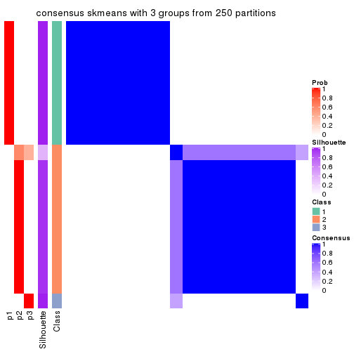
consensus_heatmap(res, k = 4)
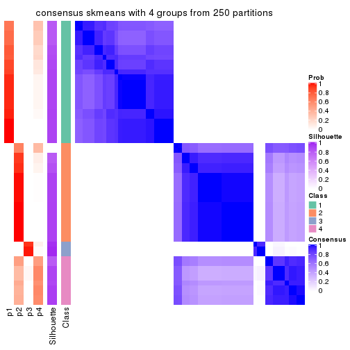
consensus_heatmap(res, k = 5)
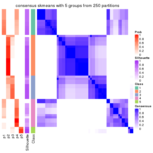
consensus_heatmap(res, k = 6)
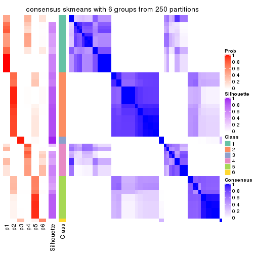
Heatmaps for the membership of samples in all partitions to see how consistent they are:
membership_heatmap(res, k = 2)

membership_heatmap(res, k = 3)
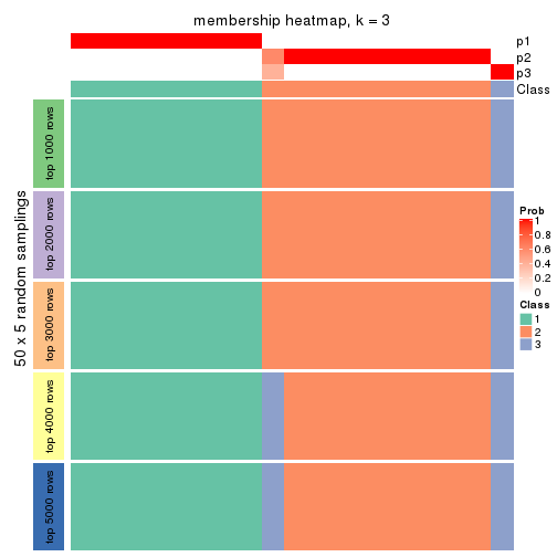
membership_heatmap(res, k = 4)
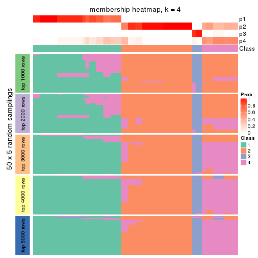
membership_heatmap(res, k = 5)
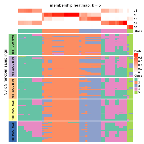
membership_heatmap(res, k = 6)
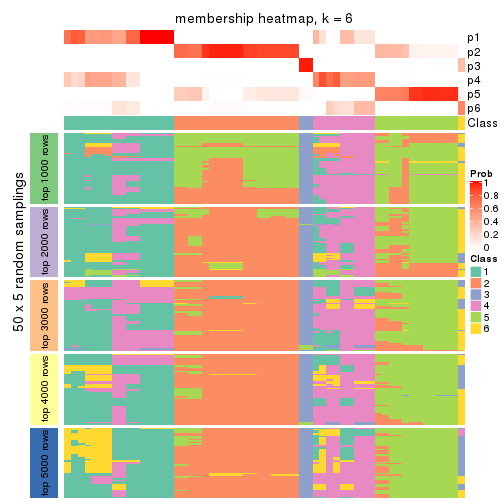
As soon as we have had the classes for columns, we can look for signatures which are significantly different between classes which can be candidate marks for certain classes. Following are the heatmaps for signatures.
Signature heatmaps where rows are scaled:
get_signatures(res, k = 2)

get_signatures(res, k = 3)
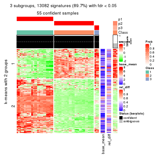
get_signatures(res, k = 4)
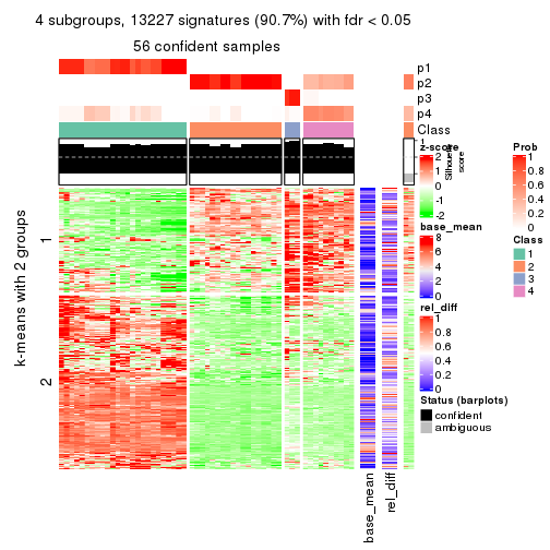
get_signatures(res, k = 5)
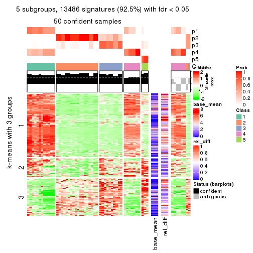
get_signatures(res, k = 6)
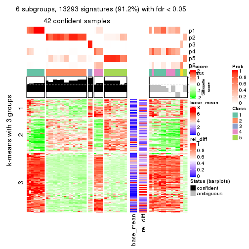
Signature heatmaps where rows are not scaled:
get_signatures(res, k = 2, scale_rows = FALSE)

get_signatures(res, k = 3, scale_rows = FALSE)
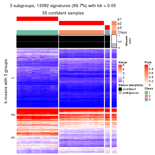
get_signatures(res, k = 4, scale_rows = FALSE)
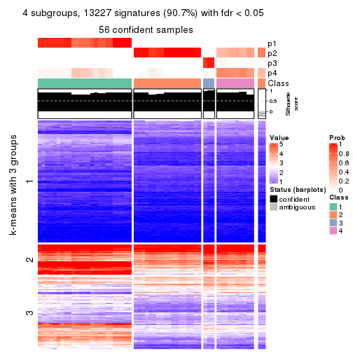
get_signatures(res, k = 5, scale_rows = FALSE)
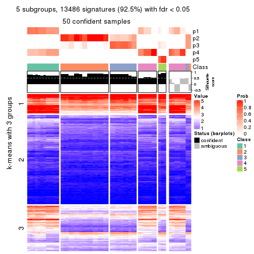
get_signatures(res, k = 6, scale_rows = FALSE)
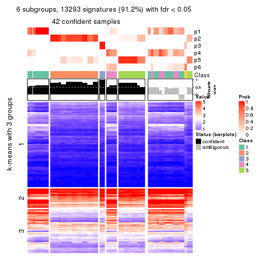
Compare the overlap of signatures from different k:
compare_signatures(res)
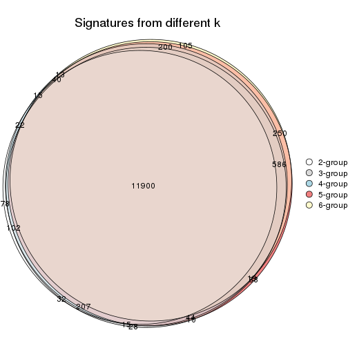
get_signature() returns a data frame invisibly. TO get the list of signatures, the function
call should be assigned to a variable explicitly. In following code, if plot argument is set
to FALSE, no heatmap is plotted while only the differential analysis is performed.
# code only for demonstration
tb = get_signature(res, k = ..., plot = FALSE)
An example of the output of tb is:
#> which_row fdr mean_1 mean_2 scaled_mean_1 scaled_mean_2 km
#> 1 38 0.042760348 8.373488 9.131774 -0.5533452 0.5164555 1
#> 2 40 0.018707592 7.106213 8.469186 -0.6173731 0.5762149 1
#> 3 55 0.019134737 10.221463 11.207825 -0.6159697 0.5749050 1
#> 4 59 0.006059896 5.921854 7.869574 -0.6899429 0.6439467 1
#> 5 60 0.018055526 8.928898 10.211722 -0.6204761 0.5791110 1
#> 6 98 0.009384629 15.714769 14.887706 0.6635654 -0.6193277 2
...
The columns in tb are:
which_row: row indices corresponding to the input matrix.fdr: FDR for the differential test. mean_x: The mean value in group x.scaled_mean_x: The mean value in group x after rows are scaled.km: Row groups if k-means clustering is applied to rows.UMAP plot which shows how samples are separated.
dimension_reduction(res, k = 2, method = "UMAP")

dimension_reduction(res, k = 3, method = "UMAP")
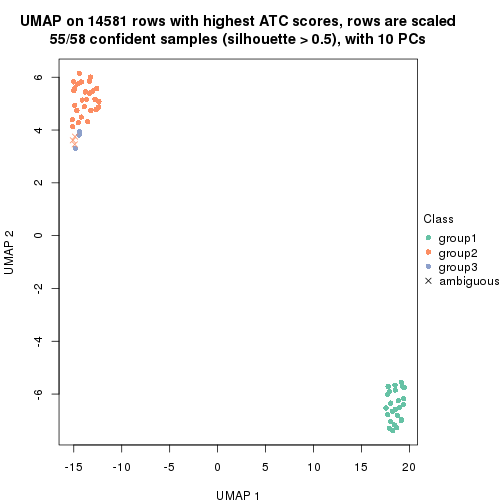
dimension_reduction(res, k = 4, method = "UMAP")
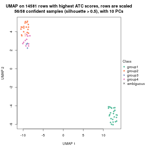
dimension_reduction(res, k = 5, method = "UMAP")
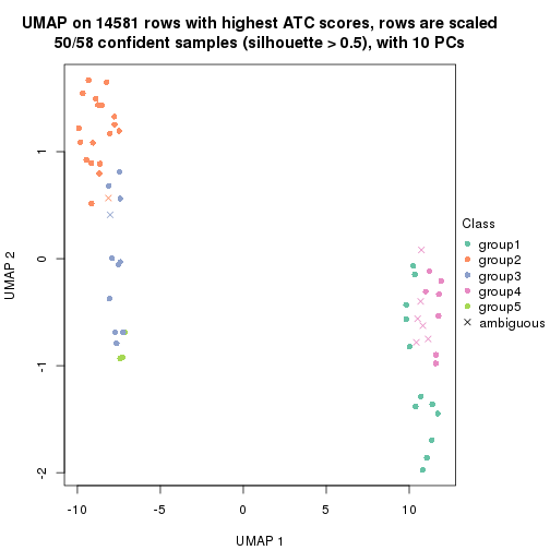
dimension_reduction(res, k = 6, method = "UMAP")

Following heatmap shows how subgroups are split when increasing k:
collect_classes(res)
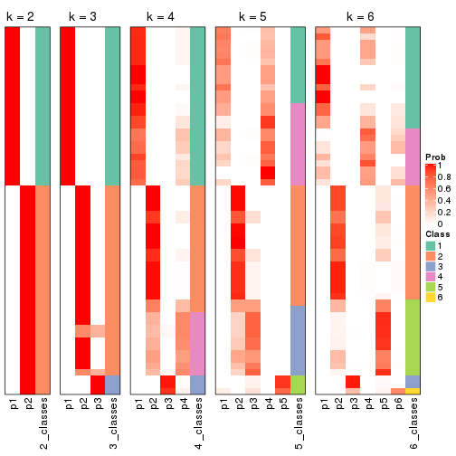
If matrix rows can be associated to genes, consider to use functional_enrichment(res,
...) to perform function enrichment for the signature genes. See this vignette for more detailed explanations.
The object with results only for a single top-value method and a single partition method can be extracted as:
res = res_list["ATC", "pam"]
# you can also extract it by
# res = res_list["ATC:pam"]
A summary of res and all the functions that can be applied to it:
res
#> A 'ConsensusPartition' object with k = 2, 3, 4, 5, 6.
#> On a matrix with 14581 rows and 58 columns.
#> Top rows (1000, 2000, 3000, 4000, 5000) are extracted by 'ATC' method.
#> Subgroups are detected by 'pam' method.
#> Performed in total 1250 partitions by row resampling.
#> Best k for subgroups seems to be 6.
#>
#> Following methods can be applied to this 'ConsensusPartition' object:
#> [1] "cola_report" "collect_classes" "collect_plots"
#> [4] "collect_stats" "colnames" "compare_signatures"
#> [7] "consensus_heatmap" "dimension_reduction" "functional_enrichment"
#> [10] "get_anno_col" "get_anno" "get_classes"
#> [13] "get_consensus" "get_matrix" "get_membership"
#> [16] "get_param" "get_signatures" "get_stats"
#> [19] "is_best_k" "is_stable_k" "membership_heatmap"
#> [22] "ncol" "nrow" "plot_ecdf"
#> [25] "rownames" "select_partition_number" "show"
#> [28] "suggest_best_k" "test_to_known_factors"
collect_plots() function collects all the plots made from res for all k (number of partitions)
into one single page to provide an easy and fast comparison between different k.
collect_plots(res)
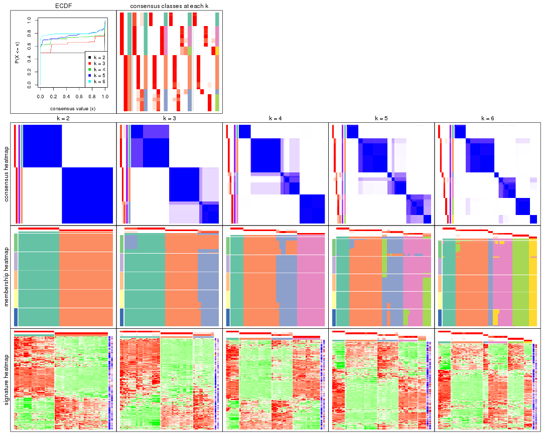
The plots are:
k and the heatmap of
predicted classes for each k.k.k.k.All the plots in panels can be made by individual functions and they are plotted later in this section.
select_partition_number() produces several plots showing different
statistics for choosing “optimized” k. There are following statistics:
k;k, the area increased is defined as \(A_k - A_{k-1}\).The detailed explanations of these statistics can be found in the cola vignette.
Generally speaking, lower PAC score, higher mean silhouette score or higher
concordance corresponds to better partition. Rand index and Jaccard index
measure how similar the current partition is compared to partition with k-1.
If they are too similar, we won't accept k is better than k-1.
select_partition_number(res)
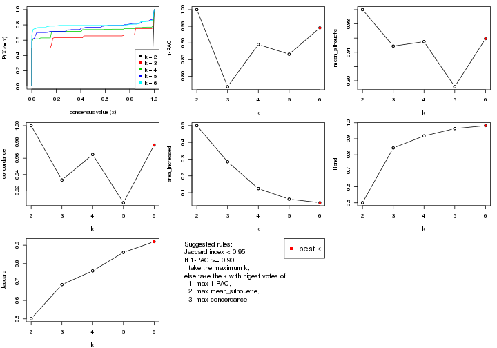
The numeric values for all these statistics can be obtained by get_stats().
get_stats(res)
#> k 1-PAC mean_silhouette concordance area_increased Rand Jaccard
#> 2 2 1.000 1.000 1.000 0.4996 0.501 0.501
#> 3 3 0.769 0.949 0.933 0.2842 0.843 0.686
#> 4 4 0.895 0.955 0.965 0.1243 0.918 0.761
#> 5 5 0.866 0.892 0.905 0.0611 0.964 0.861
#> 6 6 0.945 0.959 0.976 0.0403 0.982 0.919
suggest_best_k() suggests the best \(k\) based on these statistics. The rules are as follows:
suggest_best_k(res)
#> [1] 6
#> attr(,"optional")
#> [1] 2
There is also optional best \(k\) = 2 that is worth to check.
Following shows the table of the partitions (You need to click the show/hide
code output link to see it). The membership matrix (columns with name p*)
is inferred by
clue::cl_consensus()
function with the SE method. Basically the value in the membership matrix
represents the probability to belong to a certain group. The finall class
label for an item is determined with the group with highest probability it
belongs to.
In get_classes() function, the entropy is calculated from the membership
matrix and the silhouette score is calculated from the consensus matrix.
cbind(get_classes(res, k = 2), get_membership(res, k = 2))
#> class entropy silhouette p1 p2
#> ERR789082 2 0 1 0 1
#> ERR789083 2 0 1 0 1
#> ERR789191 2 0 1 0 1
#> ERR789192 2 0 1 0 1
#> ERR789213 1 0 1 1 0
#> ERR789385 1 0 1 1 0
#> ERR789393 1 0 1 1 0
#> ERR789394 1 0 1 1 0
#> ERR789193 2 0 1 0 1
#> ERR789194 2 0 1 0 1
#> ERR789195 2 0 1 0 1
#> ERR789196 2 0 1 0 1
#> ERR789388 1 0 1 1 0
#> ERR789197 2 0 1 0 1
#> ERR789198 2 0 1 0 1
#> ERR789214 1 0 1 1 0
#> ERR789397 1 0 1 1 0
#> ERR789398 1 0 1 1 0
#> ERR789199 2 0 1 0 1
#> ERR789200 2 0 1 0 1
#> ERR789201 2 0 1 0 1
#> ERR789202 2 0 1 0 1
#> ERR789215 1 0 1 1 0
#> ERR789203 2 0 1 0 1
#> ERR789204 2 0 1 0 1
#> ERR789383 1 0 1 1 0
#> ERR789205 2 0 1 0 1
#> ERR789206 2 0 1 0 1
#> ERR789399 1 0 1 1 0
#> ERR789400 1 0 1 1 0
#> ERR789207 2 0 1 0 1
#> ERR789208 2 0 1 0 1
#> ERR789209 2 0 1 0 1
#> ERR789210 2 0 1 0 1
#> ERR789211 2 0 1 0 1
#> ERR789212 2 0 1 0 1
#> ERR789386 1 0 1 1 0
#> ERR789076 2 0 1 0 1
#> ERR789077 2 0 1 0 1
#> ERR789384 1 0 1 1 0
#> ERR789078 2 0 1 0 1
#> ERR789079 2 0 1 0 1
#> ERR789216 1 0 1 1 0
#> ERR789080 2 0 1 0 1
#> ERR789387 1 0 1 1 0
#> ERR789081 2 0 1 0 1
#> ERR789064 2 0 1 0 1
#> ERR779485 2 0 1 0 1
#> ERR789065 2 0 1 0 1
#> ERR789401 1 0 1 1 0
#> ERR789402 1 0 1 1 0
#> ERR789403 1 0 1 1 0
#> ERR789389 1 0 1 1 0
#> ERR789395 1 0 1 1 0
#> ERR789396 1 0 1 1 0
#> ERR789390 1 0 1 1 0
#> ERR789391 1 0 1 1 0
#> ERR789392 1 0 1 1 0
cbind(get_classes(res, k = 3), get_membership(res, k = 3))
#> class entropy silhouette p1 p2 p3
#> ERR789082 2 0.0000 0.999 0.000 1.000 0.000
#> ERR789083 2 0.0000 0.999 0.000 1.000 0.000
#> ERR789191 2 0.0000 0.999 0.000 1.000 0.000
#> ERR789192 2 0.0000 0.999 0.000 1.000 0.000
#> ERR789213 1 0.0000 0.956 1.000 0.000 0.000
#> ERR789385 1 0.0000 0.956 1.000 0.000 0.000
#> ERR789393 1 0.0000 0.956 1.000 0.000 0.000
#> ERR789394 1 0.0000 0.956 1.000 0.000 0.000
#> ERR789193 3 0.3941 0.942 0.000 0.156 0.844
#> ERR789194 3 0.3941 0.942 0.000 0.156 0.844
#> ERR789195 3 0.4062 0.945 0.000 0.164 0.836
#> ERR789196 3 0.4062 0.945 0.000 0.164 0.836
#> ERR789388 1 0.0000 0.956 1.000 0.000 0.000
#> ERR789197 2 0.0000 0.999 0.000 1.000 0.000
#> ERR789198 2 0.0000 0.999 0.000 1.000 0.000
#> ERR789214 1 0.0000 0.956 1.000 0.000 0.000
#> ERR789397 1 0.0000 0.956 1.000 0.000 0.000
#> ERR789398 1 0.0000 0.956 1.000 0.000 0.000
#> ERR789199 2 0.0000 0.999 0.000 1.000 0.000
#> ERR789200 2 0.0000 0.999 0.000 1.000 0.000
#> ERR789201 3 0.6180 0.601 0.000 0.416 0.584
#> ERR789202 3 0.6180 0.601 0.000 0.416 0.584
#> ERR789215 1 0.0000 0.956 1.000 0.000 0.000
#> ERR789203 3 0.4062 0.945 0.000 0.164 0.836
#> ERR789204 3 0.4062 0.945 0.000 0.164 0.836
#> ERR789383 1 0.3941 0.903 0.844 0.000 0.156
#> ERR789205 3 0.4062 0.945 0.000 0.164 0.836
#> ERR789206 3 0.4062 0.945 0.000 0.164 0.836
#> ERR789399 1 0.0000 0.956 1.000 0.000 0.000
#> ERR789400 1 0.0000 0.956 1.000 0.000 0.000
#> ERR789207 2 0.0000 0.999 0.000 1.000 0.000
#> ERR789208 2 0.0000 0.999 0.000 1.000 0.000
#> ERR789209 2 0.0000 0.999 0.000 1.000 0.000
#> ERR789210 2 0.0000 0.999 0.000 1.000 0.000
#> ERR789211 2 0.0000 0.999 0.000 1.000 0.000
#> ERR789212 2 0.0000 0.999 0.000 1.000 0.000
#> ERR789386 1 0.0000 0.956 1.000 0.000 0.000
#> ERR789076 3 0.4062 0.945 0.000 0.164 0.836
#> ERR789077 2 0.0000 0.999 0.000 1.000 0.000
#> ERR789384 1 0.0000 0.956 1.000 0.000 0.000
#> ERR789078 2 0.0000 0.999 0.000 1.000 0.000
#> ERR789079 2 0.0000 0.999 0.000 1.000 0.000
#> ERR789216 1 0.0000 0.956 1.000 0.000 0.000
#> ERR789080 2 0.0747 0.979 0.000 0.984 0.016
#> ERR789387 1 0.3941 0.903 0.844 0.000 0.156
#> ERR789081 2 0.0000 0.999 0.000 1.000 0.000
#> ERR789064 2 0.0000 0.999 0.000 1.000 0.000
#> ERR779485 3 0.3941 0.942 0.000 0.156 0.844
#> ERR789065 3 0.4002 0.944 0.000 0.160 0.840
#> ERR789401 1 0.3941 0.903 0.844 0.000 0.156
#> ERR789402 1 0.3941 0.903 0.844 0.000 0.156
#> ERR789403 1 0.3941 0.903 0.844 0.000 0.156
#> ERR789389 1 0.3941 0.903 0.844 0.000 0.156
#> ERR789395 1 0.3941 0.903 0.844 0.000 0.156
#> ERR789396 1 0.3941 0.903 0.844 0.000 0.156
#> ERR789390 1 0.0000 0.956 1.000 0.000 0.000
#> ERR789391 1 0.0000 0.956 1.000 0.000 0.000
#> ERR789392 1 0.0000 0.956 1.000 0.000 0.000
cbind(get_classes(res, k = 4), get_membership(res, k = 4))
#> class entropy silhouette p1 p2 p3 p4
#> ERR789082 2 0.0000 0.999 0.000 1.000 0.000 0.000
#> ERR789083 2 0.0000 0.999 0.000 1.000 0.000 0.000
#> ERR789191 2 0.0000 0.999 0.000 1.000 0.000 0.000
#> ERR789192 2 0.0000 0.999 0.000 1.000 0.000 0.000
#> ERR789213 4 0.0000 0.998 0.000 0.000 0.000 1.000
#> ERR789385 4 0.0000 0.998 0.000 0.000 0.000 1.000
#> ERR789393 4 0.0000 0.998 0.000 0.000 0.000 1.000
#> ERR789394 4 0.0000 0.998 0.000 0.000 0.000 1.000
#> ERR789193 3 0.0000 0.783 0.000 0.000 1.000 0.000
#> ERR789194 3 0.0000 0.783 0.000 0.000 1.000 0.000
#> ERR789195 3 0.3172 0.884 0.000 0.160 0.840 0.000
#> ERR789196 3 0.3172 0.884 0.000 0.160 0.840 0.000
#> ERR789388 4 0.0188 0.998 0.004 0.000 0.000 0.996
#> ERR789197 2 0.0000 0.999 0.000 1.000 0.000 0.000
#> ERR789198 2 0.0000 0.999 0.000 1.000 0.000 0.000
#> ERR789214 4 0.0000 0.998 0.000 0.000 0.000 1.000
#> ERR789397 4 0.0188 0.998 0.004 0.000 0.000 0.996
#> ERR789398 4 0.0188 0.998 0.004 0.000 0.000 0.996
#> ERR789199 2 0.0000 0.999 0.000 1.000 0.000 0.000
#> ERR789200 2 0.0000 0.999 0.000 1.000 0.000 0.000
#> ERR789201 3 0.4888 0.549 0.000 0.412 0.588 0.000
#> ERR789202 3 0.4888 0.549 0.000 0.412 0.588 0.000
#> ERR789215 4 0.0188 0.998 0.004 0.000 0.000 0.996
#> ERR789203 3 0.3172 0.884 0.000 0.160 0.840 0.000
#> ERR789204 3 0.3172 0.884 0.000 0.160 0.840 0.000
#> ERR789383 1 0.0000 1.000 1.000 0.000 0.000 0.000
#> ERR789205 3 0.3172 0.884 0.000 0.160 0.840 0.000
#> ERR789206 3 0.3172 0.884 0.000 0.160 0.840 0.000
#> ERR789399 4 0.0188 0.998 0.004 0.000 0.000 0.996
#> ERR789400 4 0.0188 0.998 0.004 0.000 0.000 0.996
#> ERR789207 2 0.0000 0.999 0.000 1.000 0.000 0.000
#> ERR789208 2 0.0000 0.999 0.000 1.000 0.000 0.000
#> ERR789209 2 0.0000 0.999 0.000 1.000 0.000 0.000
#> ERR789210 2 0.0000 0.999 0.000 1.000 0.000 0.000
#> ERR789211 2 0.0000 0.999 0.000 1.000 0.000 0.000
#> ERR789212 2 0.0000 0.999 0.000 1.000 0.000 0.000
#> ERR789386 4 0.0000 0.998 0.000 0.000 0.000 1.000
#> ERR789076 3 0.3172 0.884 0.000 0.160 0.840 0.000
#> ERR789077 2 0.0000 0.999 0.000 1.000 0.000 0.000
#> ERR789384 4 0.0000 0.998 0.000 0.000 0.000 1.000
#> ERR789078 2 0.0000 0.999 0.000 1.000 0.000 0.000
#> ERR789079 2 0.0000 0.999 0.000 1.000 0.000 0.000
#> ERR789216 4 0.0000 0.998 0.000 0.000 0.000 1.000
#> ERR789080 2 0.0592 0.980 0.000 0.984 0.016 0.000
#> ERR789387 1 0.0000 1.000 1.000 0.000 0.000 0.000
#> ERR789081 2 0.0000 0.999 0.000 1.000 0.000 0.000
#> ERR789064 2 0.0000 0.999 0.000 1.000 0.000 0.000
#> ERR779485 3 0.0000 0.783 0.000 0.000 1.000 0.000
#> ERR789065 3 0.1716 0.832 0.000 0.064 0.936 0.000
#> ERR789401 1 0.0000 1.000 1.000 0.000 0.000 0.000
#> ERR789402 1 0.0000 1.000 1.000 0.000 0.000 0.000
#> ERR789403 1 0.0000 1.000 1.000 0.000 0.000 0.000
#> ERR789389 1 0.0000 1.000 1.000 0.000 0.000 0.000
#> ERR789395 1 0.0000 1.000 1.000 0.000 0.000 0.000
#> ERR789396 1 0.0000 1.000 1.000 0.000 0.000 0.000
#> ERR789390 4 0.0188 0.998 0.004 0.000 0.000 0.996
#> ERR789391 4 0.0188 0.998 0.004 0.000 0.000 0.996
#> ERR789392 4 0.0000 0.998 0.000 0.000 0.000 1.000
cbind(get_classes(res, k = 5), get_membership(res, k = 5))
#> class entropy silhouette p1 p2 p3 p4 p5
#> ERR789082 2 0.0000 0.978 0.000 1.000 0.000 0.000 0.000
#> ERR789083 2 0.0000 0.978 0.000 1.000 0.000 0.000 0.000
#> ERR789191 2 0.0000 0.978 0.000 1.000 0.000 0.000 0.000
#> ERR789192 2 0.0000 0.978 0.000 1.000 0.000 0.000 0.000
#> ERR789213 5 0.4182 1.000 0.000 0.000 0.000 0.400 0.600
#> ERR789385 5 0.4182 1.000 0.000 0.000 0.000 0.400 0.600
#> ERR789393 5 0.4182 1.000 0.000 0.000 0.000 0.400 0.600
#> ERR789394 5 0.4182 1.000 0.000 0.000 0.000 0.400 0.600
#> ERR789193 3 0.4182 0.625 0.000 0.000 0.600 0.000 0.400
#> ERR789194 3 0.4182 0.625 0.000 0.000 0.600 0.000 0.400
#> ERR789195 3 0.0794 0.848 0.000 0.028 0.972 0.000 0.000
#> ERR789196 3 0.0794 0.848 0.000 0.028 0.972 0.000 0.000
#> ERR789388 4 0.0000 0.876 0.000 0.000 0.000 1.000 0.000
#> ERR789197 2 0.0000 0.978 0.000 1.000 0.000 0.000 0.000
#> ERR789198 2 0.0000 0.978 0.000 1.000 0.000 0.000 0.000
#> ERR789214 4 0.0880 0.869 0.000 0.000 0.000 0.968 0.032
#> ERR789397 4 0.0880 0.869 0.000 0.000 0.000 0.968 0.032
#> ERR789398 4 0.0880 0.869 0.000 0.000 0.000 0.968 0.032
#> ERR789199 2 0.0000 0.978 0.000 1.000 0.000 0.000 0.000
#> ERR789200 2 0.0000 0.978 0.000 1.000 0.000 0.000 0.000
#> ERR789201 3 0.3684 0.606 0.000 0.280 0.720 0.000 0.000
#> ERR789202 3 0.3684 0.606 0.000 0.280 0.720 0.000 0.000
#> ERR789215 4 0.1197 0.848 0.000 0.000 0.000 0.952 0.048
#> ERR789203 3 0.0794 0.848 0.000 0.028 0.972 0.000 0.000
#> ERR789204 3 0.0794 0.848 0.000 0.028 0.972 0.000 0.000
#> ERR789383 1 0.0000 0.996 1.000 0.000 0.000 0.000 0.000
#> ERR789205 3 0.0794 0.848 0.000 0.028 0.972 0.000 0.000
#> ERR789206 3 0.0794 0.848 0.000 0.028 0.972 0.000 0.000
#> ERR789399 4 0.0000 0.876 0.000 0.000 0.000 1.000 0.000
#> ERR789400 4 0.0000 0.876 0.000 0.000 0.000 1.000 0.000
#> ERR789207 2 0.0290 0.978 0.000 0.992 0.008 0.000 0.000
#> ERR789208 2 0.0290 0.978 0.000 0.992 0.008 0.000 0.000
#> ERR789209 2 0.0290 0.978 0.000 0.992 0.008 0.000 0.000
#> ERR789210 2 0.0290 0.978 0.000 0.992 0.008 0.000 0.000
#> ERR789211 2 0.0290 0.978 0.000 0.992 0.008 0.000 0.000
#> ERR789212 2 0.0290 0.978 0.000 0.992 0.008 0.000 0.000
#> ERR789386 4 0.3003 0.626 0.000 0.000 0.000 0.812 0.188
#> ERR789076 3 0.0794 0.848 0.000 0.028 0.972 0.000 0.000
#> ERR789077 2 0.0000 0.978 0.000 1.000 0.000 0.000 0.000
#> ERR789384 4 0.3274 0.580 0.000 0.000 0.000 0.780 0.220
#> ERR789078 2 0.0290 0.978 0.000 0.992 0.008 0.000 0.000
#> ERR789079 2 0.2074 0.892 0.000 0.896 0.104 0.000 0.000
#> ERR789216 4 0.3210 0.594 0.000 0.000 0.000 0.788 0.212
#> ERR789080 2 0.2230 0.878 0.000 0.884 0.116 0.000 0.000
#> ERR789387 1 0.0880 0.968 0.968 0.000 0.000 0.032 0.000
#> ERR789081 2 0.2074 0.892 0.000 0.896 0.104 0.000 0.000
#> ERR789064 2 0.0000 0.978 0.000 1.000 0.000 0.000 0.000
#> ERR779485 3 0.4182 0.625 0.000 0.000 0.600 0.000 0.400
#> ERR789065 3 0.0290 0.835 0.000 0.008 0.992 0.000 0.000
#> ERR789401 1 0.0000 0.996 1.000 0.000 0.000 0.000 0.000
#> ERR789402 1 0.0000 0.996 1.000 0.000 0.000 0.000 0.000
#> ERR789403 1 0.0000 0.996 1.000 0.000 0.000 0.000 0.000
#> ERR789389 1 0.0000 0.996 1.000 0.000 0.000 0.000 0.000
#> ERR789395 1 0.0000 0.996 1.000 0.000 0.000 0.000 0.000
#> ERR789396 1 0.0000 0.996 1.000 0.000 0.000 0.000 0.000
#> ERR789390 4 0.0000 0.876 0.000 0.000 0.000 1.000 0.000
#> ERR789391 4 0.0000 0.876 0.000 0.000 0.000 1.000 0.000
#> ERR789392 5 0.4182 1.000 0.000 0.000 0.000 0.400 0.600
cbind(get_classes(res, k = 6), get_membership(res, k = 6))
#> class entropy silhouette p1 p2 p3 p4 p5 p6
#> ERR789082 2 0.000 0.974 0.000 1.000 0.000 0.000 0.000 0.000
#> ERR789083 2 0.000 0.974 0.000 1.000 0.000 0.000 0.000 0.000
#> ERR789191 2 0.000 0.974 0.000 1.000 0.000 0.000 0.000 0.000
#> ERR789192 2 0.000 0.974 0.000 1.000 0.000 0.000 0.000 0.000
#> ERR789213 6 0.000 0.988 0.000 0.000 0.000 0.000 0.000 1.000
#> ERR789385 6 0.026 0.997 0.000 0.000 0.000 0.008 0.000 0.992
#> ERR789393 6 0.026 0.997 0.000 0.000 0.000 0.008 0.000 0.992
#> ERR789394 6 0.026 0.997 0.000 0.000 0.000 0.008 0.000 0.992
#> ERR789193 3 0.026 1.000 0.000 0.000 0.992 0.000 0.008 0.000
#> ERR789194 3 0.026 1.000 0.000 0.000 0.992 0.000 0.008 0.000
#> ERR789195 5 0.000 0.997 0.000 0.000 0.000 0.000 1.000 0.000
#> ERR789196 5 0.000 0.997 0.000 0.000 0.000 0.000 1.000 0.000
#> ERR789388 4 0.000 0.922 0.000 0.000 0.000 1.000 0.000 0.000
#> ERR789197 2 0.000 0.974 0.000 1.000 0.000 0.000 0.000 0.000
#> ERR789198 2 0.000 0.974 0.000 1.000 0.000 0.000 0.000 0.000
#> ERR789214 4 0.079 0.920 0.000 0.000 0.000 0.968 0.000 0.032
#> ERR789397 4 0.079 0.920 0.000 0.000 0.000 0.968 0.000 0.032
#> ERR789398 4 0.079 0.920 0.000 0.000 0.000 0.968 0.000 0.032
#> ERR789199 2 0.000 0.974 0.000 1.000 0.000 0.000 0.000 0.000
#> ERR789200 2 0.000 0.974 0.000 1.000 0.000 0.000 0.000 0.000
#> ERR789201 5 0.026 0.989 0.000 0.008 0.000 0.000 0.992 0.000
#> ERR789202 5 0.026 0.989 0.000 0.008 0.000 0.000 0.992 0.000
#> ERR789215 4 0.146 0.904 0.000 0.000 0.008 0.936 0.000 0.056
#> ERR789203 5 0.000 0.997 0.000 0.000 0.000 0.000 1.000 0.000
#> ERR789204 5 0.000 0.997 0.000 0.000 0.000 0.000 1.000 0.000
#> ERR789383 1 0.000 0.993 1.000 0.000 0.000 0.000 0.000 0.000
#> ERR789205 5 0.000 0.997 0.000 0.000 0.000 0.000 1.000 0.000
#> ERR789206 5 0.000 0.997 0.000 0.000 0.000 0.000 1.000 0.000
#> ERR789399 4 0.000 0.922 0.000 0.000 0.000 1.000 0.000 0.000
#> ERR789400 4 0.000 0.922 0.000 0.000 0.000 1.000 0.000 0.000
#> ERR789207 2 0.026 0.974 0.000 0.992 0.000 0.000 0.008 0.000
#> ERR789208 2 0.026 0.974 0.000 0.992 0.000 0.000 0.008 0.000
#> ERR789209 2 0.026 0.974 0.000 0.992 0.000 0.000 0.008 0.000
#> ERR789210 2 0.026 0.974 0.000 0.992 0.000 0.000 0.008 0.000
#> ERR789211 2 0.026 0.974 0.000 0.992 0.000 0.000 0.008 0.000
#> ERR789212 2 0.026 0.974 0.000 0.992 0.000 0.000 0.008 0.000
#> ERR789386 4 0.301 0.802 0.000 0.000 0.008 0.796 0.000 0.196
#> ERR789076 5 0.000 0.997 0.000 0.000 0.000 0.000 1.000 0.000
#> ERR789077 2 0.000 0.974 0.000 1.000 0.000 0.000 0.000 0.000
#> ERR789384 4 0.324 0.784 0.000 0.000 0.008 0.764 0.000 0.228
#> ERR789078 2 0.026 0.974 0.000 0.992 0.000 0.000 0.008 0.000
#> ERR789079 2 0.205 0.871 0.000 0.880 0.000 0.000 0.120 0.000
#> ERR789216 4 0.319 0.790 0.000 0.000 0.008 0.772 0.000 0.220
#> ERR789080 2 0.222 0.853 0.000 0.864 0.000 0.000 0.136 0.000
#> ERR789387 1 0.131 0.947 0.952 0.000 0.008 0.032 0.000 0.008
#> ERR789081 2 0.205 0.871 0.000 0.880 0.000 0.000 0.120 0.000
#> ERR789064 2 0.000 0.974 0.000 1.000 0.000 0.000 0.000 0.000
#> ERR779485 3 0.026 1.000 0.000 0.000 0.992 0.000 0.008 0.000
#> ERR789065 5 0.000 0.997 0.000 0.000 0.000 0.000 1.000 0.000
#> ERR789401 1 0.000 0.993 1.000 0.000 0.000 0.000 0.000 0.000
#> ERR789402 1 0.000 0.993 1.000 0.000 0.000 0.000 0.000 0.000
#> ERR789403 1 0.000 0.993 1.000 0.000 0.000 0.000 0.000 0.000
#> ERR789389 1 0.000 0.993 1.000 0.000 0.000 0.000 0.000 0.000
#> ERR789395 1 0.000 0.993 1.000 0.000 0.000 0.000 0.000 0.000
#> ERR789396 1 0.000 0.993 1.000 0.000 0.000 0.000 0.000 0.000
#> ERR789390 4 0.000 0.922 0.000 0.000 0.000 1.000 0.000 0.000
#> ERR789391 4 0.000 0.922 0.000 0.000 0.000 1.000 0.000 0.000
#> ERR789392 6 0.026 0.997 0.000 0.000 0.000 0.008 0.000 0.992
Heatmaps for the consensus matrix. It visualizes the probability of two samples to be in a same group.
consensus_heatmap(res, k = 2)

consensus_heatmap(res, k = 3)
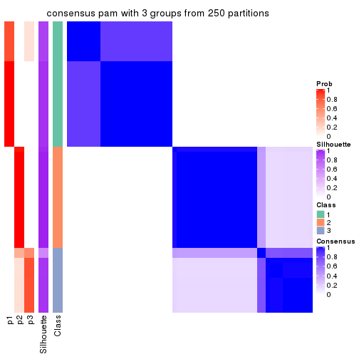
consensus_heatmap(res, k = 4)
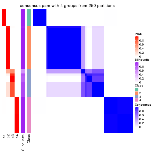
consensus_heatmap(res, k = 5)
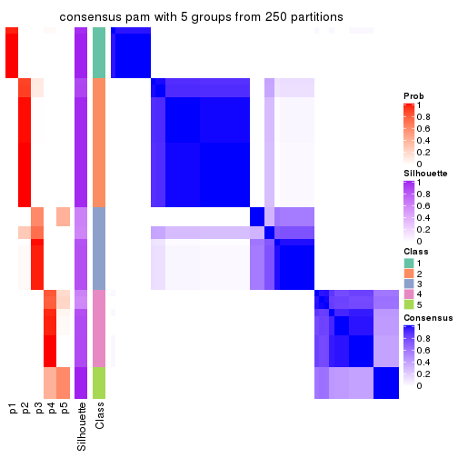
consensus_heatmap(res, k = 6)
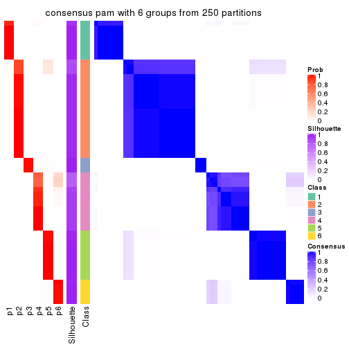
Heatmaps for the membership of samples in all partitions to see how consistent they are:
membership_heatmap(res, k = 2)

membership_heatmap(res, k = 3)
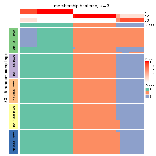
membership_heatmap(res, k = 4)
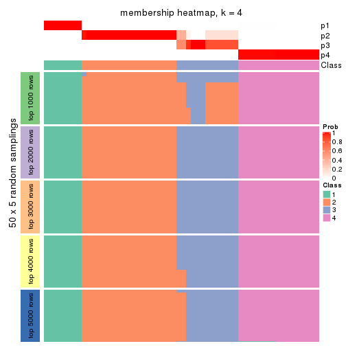
membership_heatmap(res, k = 5)
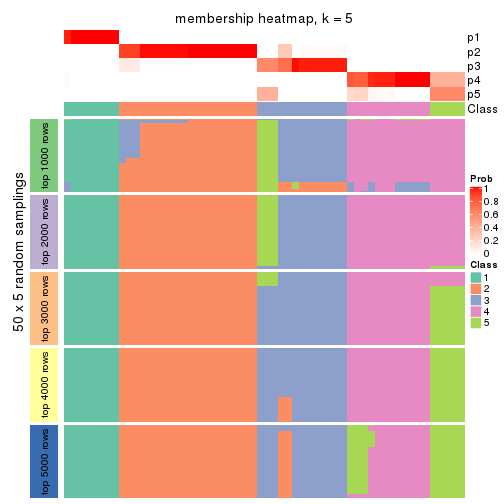
membership_heatmap(res, k = 6)
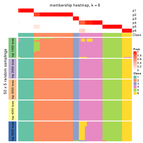
As soon as we have had the classes for columns, we can look for signatures which are significantly different between classes which can be candidate marks for certain classes. Following are the heatmaps for signatures.
Signature heatmaps where rows are scaled:
get_signatures(res, k = 2)

get_signatures(res, k = 3)
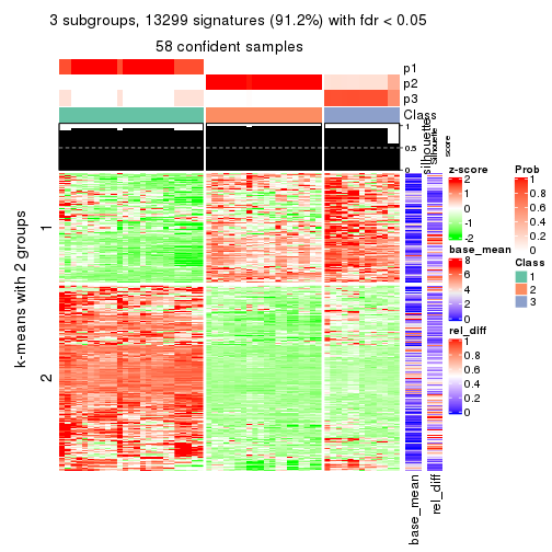
get_signatures(res, k = 4)
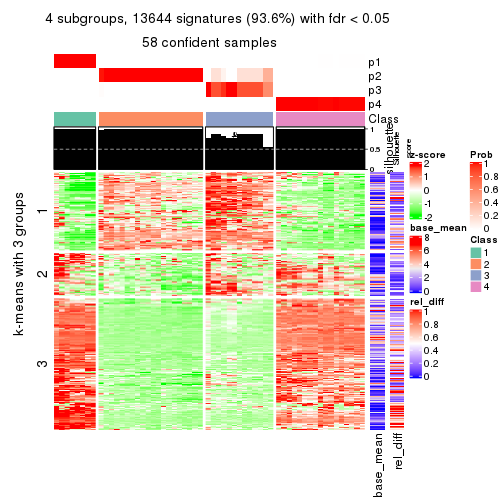
get_signatures(res, k = 5)
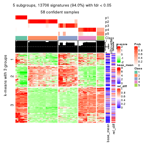
get_signatures(res, k = 6)
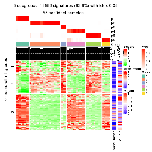
Signature heatmaps where rows are not scaled:
get_signatures(res, k = 2, scale_rows = FALSE)

get_signatures(res, k = 3, scale_rows = FALSE)
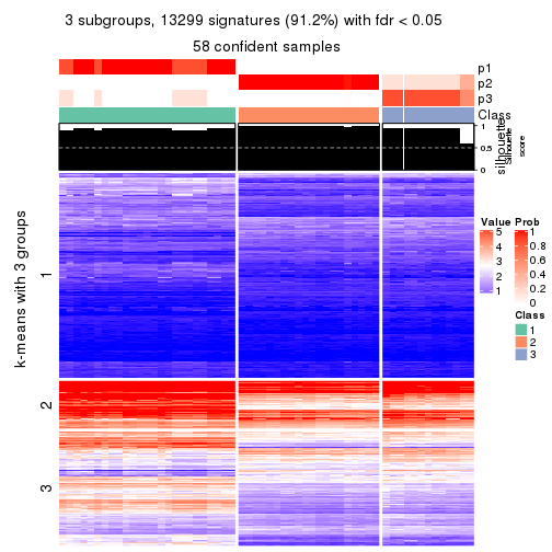
get_signatures(res, k = 4, scale_rows = FALSE)
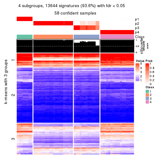
get_signatures(res, k = 5, scale_rows = FALSE)
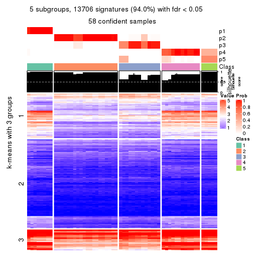
get_signatures(res, k = 6, scale_rows = FALSE)
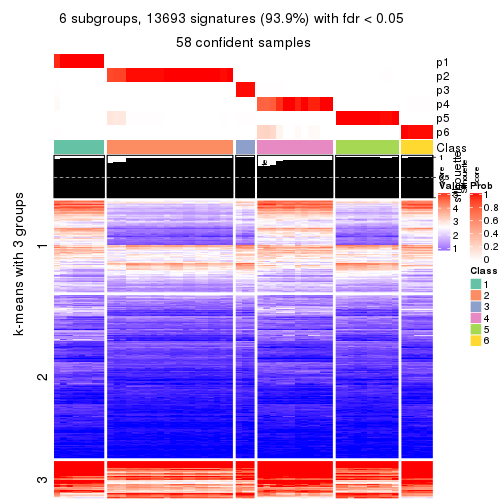
Compare the overlap of signatures from different k:
compare_signatures(res)
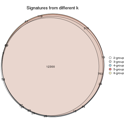
get_signature() returns a data frame invisibly. TO get the list of signatures, the function
call should be assigned to a variable explicitly. In following code, if plot argument is set
to FALSE, no heatmap is plotted while only the differential analysis is performed.
# code only for demonstration
tb = get_signature(res, k = ..., plot = FALSE)
An example of the output of tb is:
#> which_row fdr mean_1 mean_2 scaled_mean_1 scaled_mean_2 km
#> 1 38 0.042760348 8.373488 9.131774 -0.5533452 0.5164555 1
#> 2 40 0.018707592 7.106213 8.469186 -0.6173731 0.5762149 1
#> 3 55 0.019134737 10.221463 11.207825 -0.6159697 0.5749050 1
#> 4 59 0.006059896 5.921854 7.869574 -0.6899429 0.6439467 1
#> 5 60 0.018055526 8.928898 10.211722 -0.6204761 0.5791110 1
#> 6 98 0.009384629 15.714769 14.887706 0.6635654 -0.6193277 2
...
The columns in tb are:
which_row: row indices corresponding to the input matrix.fdr: FDR for the differential test. mean_x: The mean value in group x.scaled_mean_x: The mean value in group x after rows are scaled.km: Row groups if k-means clustering is applied to rows.UMAP plot which shows how samples are separated.
dimension_reduction(res, k = 2, method = "UMAP")
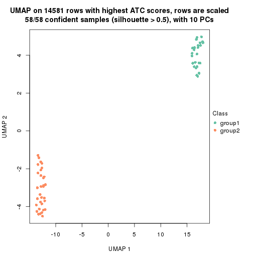
dimension_reduction(res, k = 3, method = "UMAP")
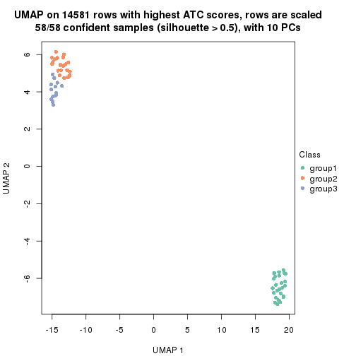
dimension_reduction(res, k = 4, method = "UMAP")
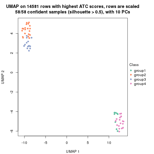
dimension_reduction(res, k = 5, method = "UMAP")
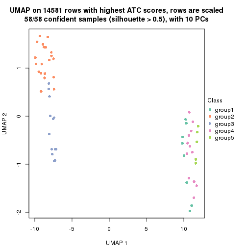
dimension_reduction(res, k = 6, method = "UMAP")
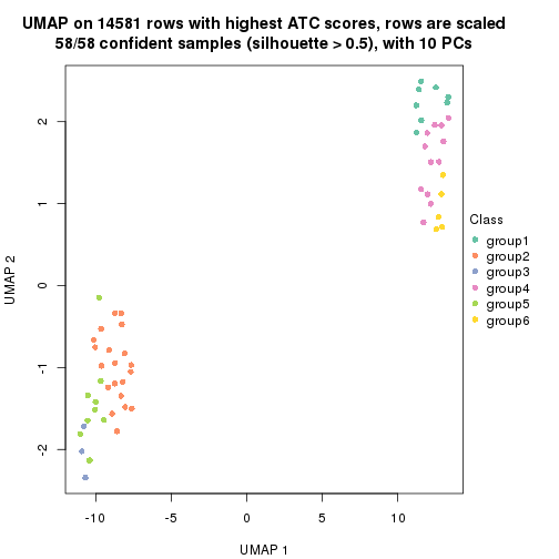
Following heatmap shows how subgroups are split when increasing k:
collect_classes(res)
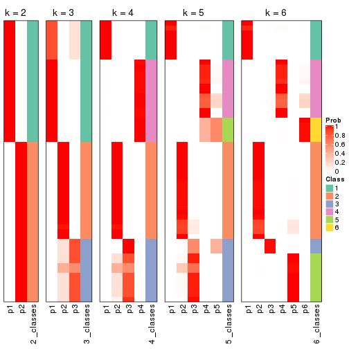
If matrix rows can be associated to genes, consider to use functional_enrichment(res,
...) to perform function enrichment for the signature genes. See this vignette for more detailed explanations.
The object with results only for a single top-value method and a single partition method can be extracted as:
res = res_list["ATC", "mclust"]
# you can also extract it by
# res = res_list["ATC:mclust"]
A summary of res and all the functions that can be applied to it:
res
#> A 'ConsensusPartition' object with k = 2, 3, 4, 5, 6.
#> On a matrix with 14581 rows and 58 columns.
#> Top rows (1000, 2000, 3000, 4000, 5000) are extracted by 'ATC' method.
#> Subgroups are detected by 'mclust' method.
#> Performed in total 1250 partitions by row resampling.
#> Best k for subgroups seems to be 2.
#>
#> Following methods can be applied to this 'ConsensusPartition' object:
#> [1] "cola_report" "collect_classes" "collect_plots"
#> [4] "collect_stats" "colnames" "compare_signatures"
#> [7] "consensus_heatmap" "dimension_reduction" "functional_enrichment"
#> [10] "get_anno_col" "get_anno" "get_classes"
#> [13] "get_consensus" "get_matrix" "get_membership"
#> [16] "get_param" "get_signatures" "get_stats"
#> [19] "is_best_k" "is_stable_k" "membership_heatmap"
#> [22] "ncol" "nrow" "plot_ecdf"
#> [25] "rownames" "select_partition_number" "show"
#> [28] "suggest_best_k" "test_to_known_factors"
collect_plots() function collects all the plots made from res for all k (number of partitions)
into one single page to provide an easy and fast comparison between different k.
collect_plots(res)
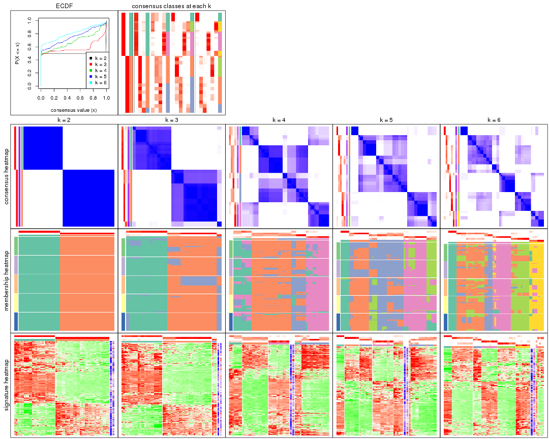
The plots are:
k and the heatmap of
predicted classes for each k.k.k.k.All the plots in panels can be made by individual functions and they are plotted later in this section.
select_partition_number() produces several plots showing different
statistics for choosing “optimized” k. There are following statistics:
k;k, the area increased is defined as \(A_k - A_{k-1}\).The detailed explanations of these statistics can be found in the cola vignette.
Generally speaking, lower PAC score, higher mean silhouette score or higher
concordance corresponds to better partition. Rand index and Jaccard index
measure how similar the current partition is compared to partition with k-1.
If they are too similar, we won't accept k is better than k-1.
select_partition_number(res)
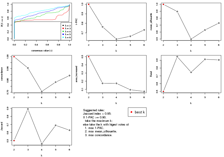
The numeric values for all these statistics can be obtained by get_stats().
get_stats(res)
#> k 1-PAC mean_silhouette concordance area_increased Rand Jaccard
#> 2 2 1.000 1.000 1.000 0.4996 0.501 0.501
#> 3 3 0.763 0.897 0.904 0.1734 0.946 0.891
#> 4 4 0.634 0.499 0.706 0.1732 0.746 0.462
#> 5 5 0.663 0.630 0.785 0.0951 0.912 0.689
#> 6 6 0.731 0.730 0.841 0.0746 0.904 0.629
suggest_best_k() suggests the best \(k\) based on these statistics. The rules are as follows:
suggest_best_k(res)
#> [1] 2
Following shows the table of the partitions (You need to click the show/hide
code output link to see it). The membership matrix (columns with name p*)
is inferred by
clue::cl_consensus()
function with the SE method. Basically the value in the membership matrix
represents the probability to belong to a certain group. The finall class
label for an item is determined with the group with highest probability it
belongs to.
In get_classes() function, the entropy is calculated from the membership
matrix and the silhouette score is calculated from the consensus matrix.
cbind(get_classes(res, k = 2), get_membership(res, k = 2))
#> class entropy silhouette p1 p2
#> ERR789082 2 0 1 0 1
#> ERR789083 2 0 1 0 1
#> ERR789191 2 0 1 0 1
#> ERR789192 2 0 1 0 1
#> ERR789213 1 0 1 1 0
#> ERR789385 1 0 1 1 0
#> ERR789393 1 0 1 1 0
#> ERR789394 1 0 1 1 0
#> ERR789193 2 0 1 0 1
#> ERR789194 2 0 1 0 1
#> ERR789195 2 0 1 0 1
#> ERR789196 2 0 1 0 1
#> ERR789388 1 0 1 1 0
#> ERR789197 2 0 1 0 1
#> ERR789198 2 0 1 0 1
#> ERR789214 1 0 1 1 0
#> ERR789397 1 0 1 1 0
#> ERR789398 1 0 1 1 0
#> ERR789199 2 0 1 0 1
#> ERR789200 2 0 1 0 1
#> ERR789201 2 0 1 0 1
#> ERR789202 2 0 1 0 1
#> ERR789215 1 0 1 1 0
#> ERR789203 2 0 1 0 1
#> ERR789204 2 0 1 0 1
#> ERR789383 1 0 1 1 0
#> ERR789205 2 0 1 0 1
#> ERR789206 2 0 1 0 1
#> ERR789399 1 0 1 1 0
#> ERR789400 1 0 1 1 0
#> ERR789207 2 0 1 0 1
#> ERR789208 2 0 1 0 1
#> ERR789209 2 0 1 0 1
#> ERR789210 2 0 1 0 1
#> ERR789211 2 0 1 0 1
#> ERR789212 2 0 1 0 1
#> ERR789386 1 0 1 1 0
#> ERR789076 2 0 1 0 1
#> ERR789077 2 0 1 0 1
#> ERR789384 1 0 1 1 0
#> ERR789078 2 0 1 0 1
#> ERR789079 2 0 1 0 1
#> ERR789216 1 0 1 1 0
#> ERR789080 2 0 1 0 1
#> ERR789387 1 0 1 1 0
#> ERR789081 2 0 1 0 1
#> ERR789064 2 0 1 0 1
#> ERR779485 2 0 1 0 1
#> ERR789065 2 0 1 0 1
#> ERR789401 1 0 1 1 0
#> ERR789402 1 0 1 1 0
#> ERR789403 1 0 1 1 0
#> ERR789389 1 0 1 1 0
#> ERR789395 1 0 1 1 0
#> ERR789396 1 0 1 1 0
#> ERR789390 1 0 1 1 0
#> ERR789391 1 0 1 1 0
#> ERR789392 1 0 1 1 0
cbind(get_classes(res, k = 3), get_membership(res, k = 3))
#> class entropy silhouette p1 p2 p3
#> ERR789082 2 0.0237 0.917 0.000 0.996 0.004
#> ERR789083 2 0.0237 0.917 0.000 0.996 0.004
#> ERR789191 2 0.0237 0.916 0.000 0.996 0.004
#> ERR789192 2 0.0237 0.916 0.000 0.996 0.004
#> ERR789213 1 0.2711 0.924 0.912 0.000 0.088
#> ERR789385 1 0.1643 0.937 0.956 0.000 0.044
#> ERR789393 1 0.1031 0.942 0.976 0.000 0.024
#> ERR789394 1 0.1031 0.942 0.976 0.000 0.024
#> ERR789193 3 0.3532 1.000 0.008 0.108 0.884
#> ERR789194 3 0.3532 1.000 0.008 0.108 0.884
#> ERR789195 2 0.5016 0.728 0.000 0.760 0.240
#> ERR789196 2 0.5016 0.728 0.000 0.760 0.240
#> ERR789388 1 0.0892 0.941 0.980 0.000 0.020
#> ERR789197 2 0.0000 0.917 0.000 1.000 0.000
#> ERR789198 2 0.0000 0.917 0.000 1.000 0.000
#> ERR789214 1 0.2711 0.924 0.912 0.000 0.088
#> ERR789397 1 0.0892 0.941 0.980 0.000 0.020
#> ERR789398 1 0.0892 0.941 0.980 0.000 0.020
#> ERR789199 2 0.0237 0.917 0.000 0.996 0.004
#> ERR789200 2 0.0237 0.917 0.000 0.996 0.004
#> ERR789201 2 0.0237 0.917 0.000 0.996 0.004
#> ERR789202 2 0.1031 0.907 0.000 0.976 0.024
#> ERR789215 1 0.2711 0.924 0.912 0.000 0.088
#> ERR789203 2 0.4702 0.757 0.000 0.788 0.212
#> ERR789204 2 0.4702 0.757 0.000 0.788 0.212
#> ERR789383 1 0.5058 0.722 0.756 0.000 0.244
#> ERR789205 2 0.5016 0.728 0.000 0.760 0.240
#> ERR789206 2 0.5016 0.728 0.000 0.760 0.240
#> ERR789399 1 0.0592 0.942 0.988 0.000 0.012
#> ERR789400 1 0.0592 0.942 0.988 0.000 0.012
#> ERR789207 2 0.0237 0.916 0.000 0.996 0.004
#> ERR789208 2 0.0237 0.916 0.000 0.996 0.004
#> ERR789209 2 0.0592 0.914 0.000 0.988 0.012
#> ERR789210 2 0.0237 0.917 0.000 0.996 0.004
#> ERR789211 2 0.0000 0.917 0.000 1.000 0.000
#> ERR789212 2 0.0000 0.917 0.000 1.000 0.000
#> ERR789386 1 0.2711 0.924 0.912 0.000 0.088
#> ERR789076 2 0.5016 0.728 0.000 0.760 0.240
#> ERR789077 2 0.0237 0.916 0.000 0.996 0.004
#> ERR789384 1 0.2711 0.924 0.912 0.000 0.088
#> ERR789078 2 0.0237 0.916 0.000 0.996 0.004
#> ERR789079 2 0.0424 0.915 0.000 0.992 0.008
#> ERR789216 1 0.2711 0.924 0.912 0.000 0.088
#> ERR789080 2 0.0424 0.915 0.000 0.992 0.008
#> ERR789387 1 0.2711 0.924 0.912 0.000 0.088
#> ERR789081 2 0.0424 0.915 0.000 0.992 0.008
#> ERR789064 2 0.0237 0.917 0.000 0.996 0.004
#> ERR779485 3 0.3532 1.000 0.008 0.108 0.884
#> ERR789065 2 0.5058 0.722 0.000 0.756 0.244
#> ERR789401 1 0.1411 0.937 0.964 0.000 0.036
#> ERR789402 1 0.1529 0.933 0.960 0.000 0.040
#> ERR789403 1 0.1529 0.936 0.960 0.000 0.040
#> ERR789389 1 0.4796 0.760 0.780 0.000 0.220
#> ERR789395 1 0.1031 0.939 0.976 0.000 0.024
#> ERR789396 1 0.1753 0.929 0.952 0.000 0.048
#> ERR789390 1 0.1031 0.941 0.976 0.000 0.024
#> ERR789391 1 0.1031 0.941 0.976 0.000 0.024
#> ERR789392 1 0.1031 0.942 0.976 0.000 0.024
cbind(get_classes(res, k = 4), get_membership(res, k = 4))
#> class entropy silhouette p1 p2 p3 p4
#> ERR789082 2 0.4998 0.816 0.000 0.512 0.488 0.000
#> ERR789083 2 0.4998 0.816 0.000 0.512 0.488 0.000
#> ERR789191 2 0.4804 0.888 0.000 0.616 0.384 0.000
#> ERR789192 2 0.4804 0.888 0.000 0.616 0.384 0.000
#> ERR789213 4 0.3311 0.751 0.172 0.000 0.000 0.828
#> ERR789385 4 0.2814 0.798 0.132 0.000 0.000 0.868
#> ERR789393 4 0.0000 0.857 0.000 0.000 0.000 1.000
#> ERR789394 4 0.0000 0.857 0.000 0.000 0.000 1.000
#> ERR789193 3 0.6123 0.128 0.372 0.056 0.572 0.000
#> ERR789194 3 0.6123 0.128 0.372 0.056 0.572 0.000
#> ERR789195 3 0.0000 0.412 0.000 0.000 1.000 0.000
#> ERR789196 3 0.0000 0.412 0.000 0.000 1.000 0.000
#> ERR789388 4 0.3649 0.688 0.204 0.000 0.000 0.796
#> ERR789197 2 0.4994 0.832 0.000 0.520 0.480 0.000
#> ERR789198 2 0.4994 0.832 0.000 0.520 0.480 0.000
#> ERR789214 4 0.3311 0.751 0.172 0.000 0.000 0.828
#> ERR789397 4 0.0000 0.857 0.000 0.000 0.000 1.000
#> ERR789398 4 0.0000 0.857 0.000 0.000 0.000 1.000
#> ERR789199 2 0.4989 0.838 0.000 0.528 0.472 0.000
#> ERR789200 2 0.4989 0.838 0.000 0.528 0.472 0.000
#> ERR789201 3 0.5151 -0.720 0.004 0.464 0.532 0.000
#> ERR789202 3 0.5126 -0.675 0.004 0.444 0.552 0.000
#> ERR789215 4 0.4830 0.292 0.392 0.000 0.000 0.608
#> ERR789203 3 0.6125 -0.506 0.048 0.436 0.516 0.000
#> ERR789204 3 0.6125 -0.506 0.048 0.436 0.516 0.000
#> ERR789383 1 0.4121 0.613 0.796 0.020 0.000 0.184
#> ERR789205 3 0.0469 0.406 0.000 0.012 0.988 0.000
#> ERR789206 3 0.0469 0.406 0.000 0.012 0.988 0.000
#> ERR789399 4 0.2530 0.785 0.112 0.000 0.000 0.888
#> ERR789400 4 0.2530 0.785 0.112 0.000 0.000 0.888
#> ERR789207 2 0.4790 0.887 0.000 0.620 0.380 0.000
#> ERR789208 2 0.4790 0.887 0.000 0.620 0.380 0.000
#> ERR789209 3 0.5360 -0.633 0.012 0.436 0.552 0.000
#> ERR789210 3 0.5353 -0.623 0.012 0.432 0.556 0.000
#> ERR789211 3 0.5360 -0.637 0.012 0.436 0.552 0.000
#> ERR789212 3 0.5383 -0.682 0.012 0.452 0.536 0.000
#> ERR789386 1 0.4843 0.419 0.604 0.000 0.000 0.396
#> ERR789076 3 0.1059 0.401 0.012 0.016 0.972 0.000
#> ERR789077 2 0.4804 0.888 0.000 0.616 0.384 0.000
#> ERR789384 1 0.4855 0.408 0.600 0.000 0.000 0.400
#> ERR789078 2 0.4790 0.887 0.000 0.620 0.380 0.000
#> ERR789079 2 0.4790 0.887 0.000 0.620 0.380 0.000
#> ERR789216 1 0.4843 0.419 0.604 0.000 0.000 0.396
#> ERR789080 2 0.4790 0.887 0.000 0.620 0.380 0.000
#> ERR789387 1 0.4382 0.552 0.704 0.000 0.000 0.296
#> ERR789081 2 0.4790 0.887 0.000 0.620 0.380 0.000
#> ERR789064 2 0.4996 0.825 0.000 0.516 0.484 0.000
#> ERR779485 3 0.6158 0.124 0.384 0.056 0.560 0.000
#> ERR789065 3 0.0188 0.412 0.000 0.004 0.996 0.000
#> ERR789401 1 0.7398 0.684 0.492 0.324 0.000 0.184
#> ERR789402 1 0.7426 0.685 0.488 0.324 0.000 0.188
#> ERR789403 1 0.7426 0.685 0.488 0.324 0.000 0.188
#> ERR789389 1 0.3806 0.610 0.824 0.020 0.000 0.156
#> ERR789395 1 0.7398 0.684 0.492 0.324 0.000 0.184
#> ERR789396 1 0.7398 0.684 0.492 0.324 0.000 0.184
#> ERR789390 4 0.0188 0.856 0.000 0.004 0.000 0.996
#> ERR789391 4 0.0188 0.856 0.000 0.004 0.000 0.996
#> ERR789392 4 0.0000 0.857 0.000 0.000 0.000 1.000
cbind(get_classes(res, k = 5), get_membership(res, k = 5))
#> class entropy silhouette p1 p2 p3 p4 p5
#> ERR789082 3 0.425 0.388 0.000 0.432 0.568 0.000 0.000
#> ERR789083 3 0.425 0.388 0.000 0.432 0.568 0.000 0.000
#> ERR789191 2 0.104 0.793 0.000 0.960 0.040 0.000 0.000
#> ERR789192 2 0.104 0.793 0.000 0.960 0.040 0.000 0.000
#> ERR789213 4 0.368 0.560 0.000 0.000 0.000 0.720 0.280
#> ERR789385 4 0.361 0.633 0.008 0.000 0.000 0.764 0.228
#> ERR789393 4 0.000 0.819 0.000 0.000 0.000 1.000 0.000
#> ERR789394 4 0.000 0.819 0.000 0.000 0.000 1.000 0.000
#> ERR789193 3 0.430 0.283 0.000 0.000 0.524 0.000 0.476
#> ERR789194 3 0.430 0.283 0.000 0.000 0.524 0.000 0.476
#> ERR789195 3 0.372 0.614 0.000 0.152 0.804 0.000 0.044
#> ERR789196 3 0.372 0.614 0.000 0.152 0.804 0.000 0.044
#> ERR789388 4 0.385 0.617 0.016 0.000 0.000 0.752 0.232
#> ERR789197 3 0.431 0.265 0.000 0.492 0.508 0.000 0.000
#> ERR789198 3 0.431 0.242 0.000 0.500 0.500 0.000 0.000
#> ERR789214 4 0.368 0.560 0.000 0.000 0.000 0.720 0.280
#> ERR789397 4 0.000 0.819 0.000 0.000 0.000 1.000 0.000
#> ERR789398 4 0.000 0.819 0.000 0.000 0.000 1.000 0.000
#> ERR789199 2 0.403 0.169 0.000 0.648 0.352 0.000 0.000
#> ERR789200 2 0.403 0.169 0.000 0.648 0.352 0.000 0.000
#> ERR789201 3 0.377 0.555 0.000 0.296 0.704 0.000 0.000
#> ERR789202 3 0.377 0.555 0.000 0.296 0.704 0.000 0.000
#> ERR789215 4 0.511 0.364 0.064 0.000 0.000 0.640 0.296
#> ERR789203 3 0.389 0.464 0.000 0.008 0.724 0.000 0.268
#> ERR789204 3 0.389 0.464 0.000 0.008 0.724 0.000 0.268
#> ERR789383 5 0.492 0.681 0.192 0.000 0.000 0.100 0.708
#> ERR789205 3 0.281 0.618 0.000 0.152 0.844 0.000 0.004
#> ERR789206 3 0.281 0.618 0.000 0.152 0.844 0.000 0.004
#> ERR789399 4 0.176 0.774 0.064 0.000 0.000 0.928 0.008
#> ERR789400 4 0.176 0.774 0.064 0.000 0.000 0.928 0.008
#> ERR789207 2 0.000 0.818 0.000 1.000 0.000 0.000 0.000
#> ERR789208 2 0.000 0.818 0.000 1.000 0.000 0.000 0.000
#> ERR789209 3 0.414 0.488 0.000 0.384 0.616 0.000 0.000
#> ERR789210 3 0.414 0.488 0.000 0.384 0.616 0.000 0.000
#> ERR789211 3 0.420 0.453 0.000 0.408 0.592 0.000 0.000
#> ERR789212 3 0.421 0.447 0.000 0.412 0.588 0.000 0.000
#> ERR789386 5 0.607 0.742 0.136 0.000 0.000 0.340 0.524
#> ERR789076 3 0.265 0.618 0.000 0.152 0.848 0.000 0.000
#> ERR789077 2 0.000 0.818 0.000 1.000 0.000 0.000 0.000
#> ERR789384 5 0.607 0.742 0.136 0.000 0.000 0.340 0.524
#> ERR789078 2 0.000 0.818 0.000 1.000 0.000 0.000 0.000
#> ERR789079 2 0.000 0.818 0.000 1.000 0.000 0.000 0.000
#> ERR789216 5 0.607 0.742 0.136 0.000 0.000 0.340 0.524
#> ERR789080 2 0.000 0.818 0.000 1.000 0.000 0.000 0.000
#> ERR789387 5 0.592 0.768 0.168 0.000 0.000 0.240 0.592
#> ERR789081 2 0.000 0.818 0.000 1.000 0.000 0.000 0.000
#> ERR789064 2 0.428 -0.222 0.000 0.548 0.452 0.000 0.000
#> ERR779485 3 0.430 0.273 0.000 0.000 0.516 0.000 0.484
#> ERR789065 3 0.387 0.605 0.000 0.140 0.800 0.000 0.060
#> ERR789401 1 0.000 1.000 1.000 0.000 0.000 0.000 0.000
#> ERR789402 1 0.000 1.000 1.000 0.000 0.000 0.000 0.000
#> ERR789403 1 0.000 1.000 1.000 0.000 0.000 0.000 0.000
#> ERR789389 5 0.492 0.681 0.192 0.000 0.000 0.100 0.708
#> ERR789395 1 0.000 1.000 1.000 0.000 0.000 0.000 0.000
#> ERR789396 1 0.000 1.000 1.000 0.000 0.000 0.000 0.000
#> ERR789390 4 0.000 0.819 0.000 0.000 0.000 1.000 0.000
#> ERR789391 4 0.000 0.819 0.000 0.000 0.000 1.000 0.000
#> ERR789392 4 0.000 0.819 0.000 0.000 0.000 1.000 0.000
cbind(get_classes(res, k = 6), get_membership(res, k = 6))
#> class entropy silhouette p1 p2 p3 p4 p5 p6
#> ERR789082 2 0.3999 0.6434 0.000 0.696 0.032 0.000 0.272 0.000
#> ERR789083 2 0.3999 0.6434 0.000 0.696 0.032 0.000 0.272 0.000
#> ERR789191 5 0.3752 0.7621 0.000 0.164 0.064 0.000 0.772 0.000
#> ERR789192 5 0.3752 0.7621 0.000 0.164 0.064 0.000 0.772 0.000
#> ERR789213 6 0.3244 0.6476 0.000 0.000 0.000 0.268 0.000 0.732
#> ERR789385 4 0.5400 -0.0123 0.064 0.000 0.020 0.488 0.000 0.428
#> ERR789393 4 0.0000 0.8987 0.000 0.000 0.000 1.000 0.000 0.000
#> ERR789394 4 0.0000 0.8987 0.000 0.000 0.000 1.000 0.000 0.000
#> ERR789193 3 0.1444 0.7795 0.000 0.072 0.928 0.000 0.000 0.000
#> ERR789194 3 0.1444 0.7795 0.000 0.072 0.928 0.000 0.000 0.000
#> ERR789195 2 0.2562 0.4732 0.000 0.828 0.172 0.000 0.000 0.000
#> ERR789196 2 0.2562 0.4732 0.000 0.828 0.172 0.000 0.000 0.000
#> ERR789388 4 0.4037 0.6557 0.064 0.000 0.000 0.736 0.000 0.200
#> ERR789197 2 0.4371 0.5650 0.000 0.620 0.036 0.000 0.344 0.000
#> ERR789198 2 0.4292 0.5739 0.000 0.628 0.032 0.000 0.340 0.000
#> ERR789214 6 0.3244 0.6476 0.000 0.000 0.000 0.268 0.000 0.732
#> ERR789397 4 0.0000 0.8987 0.000 0.000 0.000 1.000 0.000 0.000
#> ERR789398 4 0.0000 0.8987 0.000 0.000 0.000 1.000 0.000 0.000
#> ERR789199 5 0.4456 0.6109 0.000 0.268 0.064 0.000 0.668 0.000
#> ERR789200 5 0.4456 0.6109 0.000 0.268 0.064 0.000 0.668 0.000
#> ERR789201 2 0.3101 0.6979 0.000 0.756 0.000 0.000 0.244 0.000
#> ERR789202 2 0.3076 0.6991 0.000 0.760 0.000 0.000 0.240 0.000
#> ERR789215 6 0.4008 0.6696 0.064 0.000 0.000 0.196 0.000 0.740
#> ERR789203 3 0.3937 0.5870 0.000 0.424 0.572 0.000 0.004 0.000
#> ERR789204 3 0.3937 0.5870 0.000 0.424 0.572 0.000 0.004 0.000
#> ERR789383 6 0.3290 0.6094 0.252 0.000 0.004 0.000 0.000 0.744
#> ERR789205 2 0.1204 0.5862 0.000 0.944 0.056 0.000 0.000 0.000
#> ERR789206 2 0.1204 0.5862 0.000 0.944 0.056 0.000 0.000 0.000
#> ERR789399 4 0.1686 0.8610 0.064 0.000 0.000 0.924 0.000 0.012
#> ERR789400 4 0.1686 0.8610 0.064 0.000 0.000 0.924 0.000 0.012
#> ERR789207 5 0.1075 0.8499 0.000 0.048 0.000 0.000 0.952 0.000
#> ERR789208 5 0.1075 0.8499 0.000 0.048 0.000 0.000 0.952 0.000
#> ERR789209 2 0.4626 0.6652 0.000 0.652 0.076 0.000 0.272 0.000
#> ERR789210 2 0.4682 0.6637 0.000 0.640 0.076 0.000 0.284 0.000
#> ERR789211 2 0.3867 0.6548 0.000 0.660 0.012 0.000 0.328 0.000
#> ERR789212 2 0.3898 0.6487 0.000 0.652 0.012 0.000 0.336 0.000
#> ERR789386 6 0.0000 0.8049 0.000 0.000 0.000 0.000 0.000 1.000
#> ERR789076 2 0.1204 0.5906 0.000 0.944 0.056 0.000 0.000 0.000
#> ERR789077 5 0.1341 0.8504 0.000 0.024 0.028 0.000 0.948 0.000
#> ERR789384 6 0.0000 0.8049 0.000 0.000 0.000 0.000 0.000 1.000
#> ERR789078 5 0.0260 0.8567 0.000 0.008 0.000 0.000 0.992 0.000
#> ERR789079 5 0.0000 0.8570 0.000 0.000 0.000 0.000 1.000 0.000
#> ERR789216 6 0.0146 0.8044 0.000 0.000 0.004 0.000 0.000 0.996
#> ERR789080 5 0.0000 0.8570 0.000 0.000 0.000 0.000 1.000 0.000
#> ERR789387 6 0.0146 0.8044 0.000 0.000 0.004 0.000 0.000 0.996
#> ERR789081 5 0.0000 0.8570 0.000 0.000 0.000 0.000 1.000 0.000
#> ERR789064 2 0.3860 0.4567 0.000 0.528 0.000 0.000 0.472 0.000
#> ERR779485 3 0.1444 0.7795 0.000 0.072 0.928 0.000 0.000 0.000
#> ERR789065 2 0.2762 0.4250 0.000 0.804 0.196 0.000 0.000 0.000
#> ERR789401 1 0.0000 1.0000 1.000 0.000 0.000 0.000 0.000 0.000
#> ERR789402 1 0.0000 1.0000 1.000 0.000 0.000 0.000 0.000 0.000
#> ERR789403 1 0.0000 1.0000 1.000 0.000 0.000 0.000 0.000 0.000
#> ERR789389 6 0.3290 0.6094 0.252 0.000 0.004 0.000 0.000 0.744
#> ERR789395 1 0.0000 1.0000 1.000 0.000 0.000 0.000 0.000 0.000
#> ERR789396 1 0.0000 1.0000 1.000 0.000 0.000 0.000 0.000 0.000
#> ERR789390 4 0.0146 0.8977 0.004 0.000 0.000 0.996 0.000 0.000
#> ERR789391 4 0.0146 0.8977 0.004 0.000 0.000 0.996 0.000 0.000
#> ERR789392 4 0.0000 0.8987 0.000 0.000 0.000 1.000 0.000 0.000
Heatmaps for the consensus matrix. It visualizes the probability of two samples to be in a same group.
consensus_heatmap(res, k = 2)

consensus_heatmap(res, k = 3)
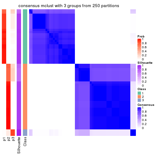
consensus_heatmap(res, k = 4)
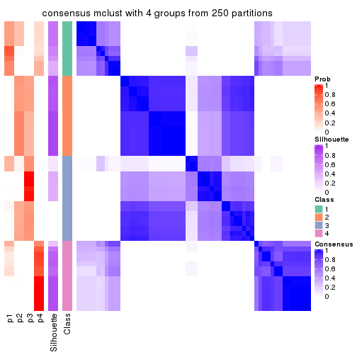
consensus_heatmap(res, k = 5)
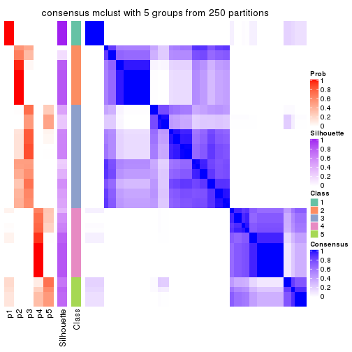
consensus_heatmap(res, k = 6)
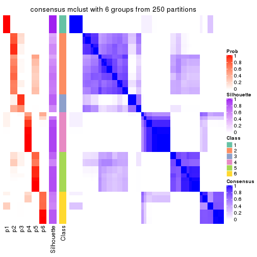
Heatmaps for the membership of samples in all partitions to see how consistent they are:
membership_heatmap(res, k = 2)

membership_heatmap(res, k = 3)
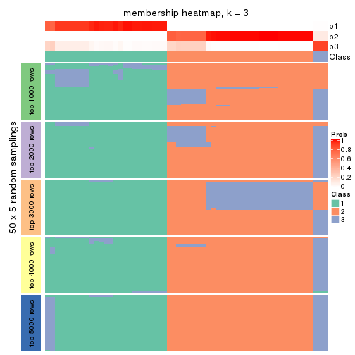
membership_heatmap(res, k = 4)
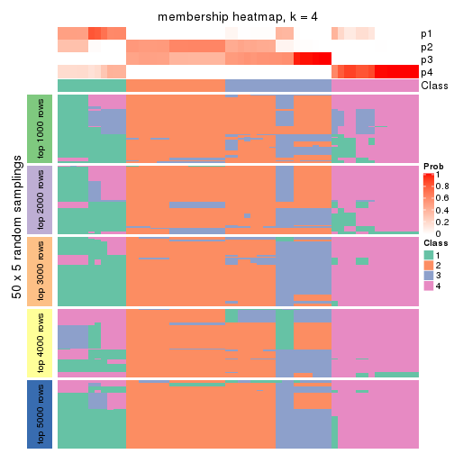
membership_heatmap(res, k = 5)
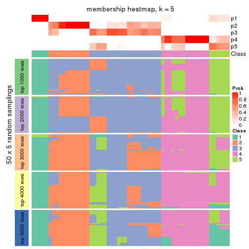
membership_heatmap(res, k = 6)
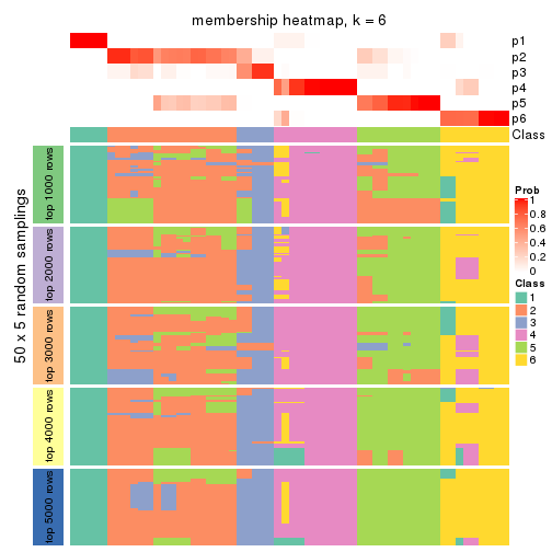
As soon as we have had the classes for columns, we can look for signatures which are significantly different between classes which can be candidate marks for certain classes. Following are the heatmaps for signatures.
Signature heatmaps where rows are scaled:
get_signatures(res, k = 2)

get_signatures(res, k = 3)
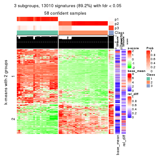
get_signatures(res, k = 4)
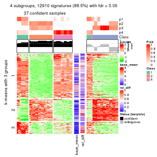
get_signatures(res, k = 5)
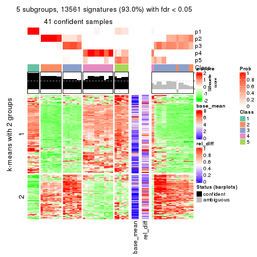
get_signatures(res, k = 6)
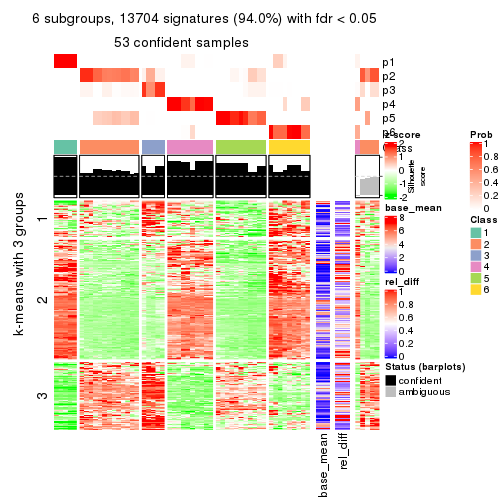
Signature heatmaps where rows are not scaled:
get_signatures(res, k = 2, scale_rows = FALSE)

get_signatures(res, k = 3, scale_rows = FALSE)
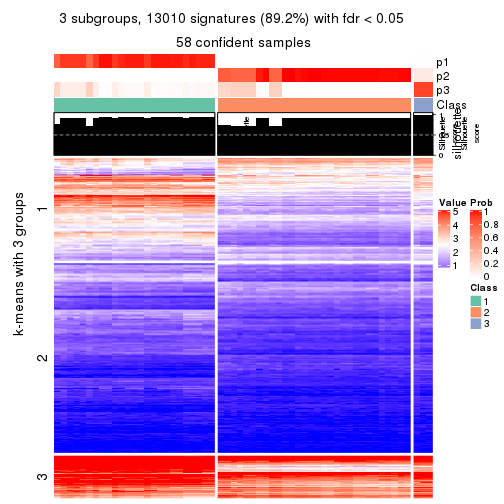
get_signatures(res, k = 4, scale_rows = FALSE)
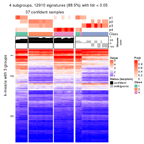
get_signatures(res, k = 5, scale_rows = FALSE)
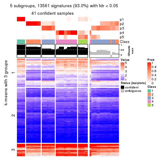
get_signatures(res, k = 6, scale_rows = FALSE)
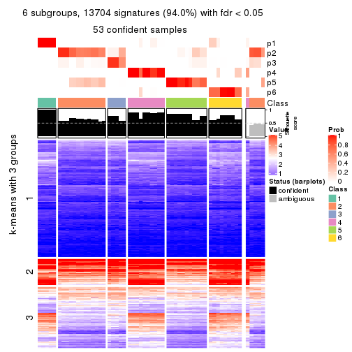
Compare the overlap of signatures from different k:
compare_signatures(res)
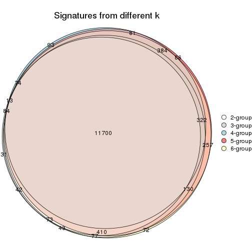
get_signature() returns a data frame invisibly. TO get the list of signatures, the function
call should be assigned to a variable explicitly. In following code, if plot argument is set
to FALSE, no heatmap is plotted while only the differential analysis is performed.
# code only for demonstration
tb = get_signature(res, k = ..., plot = FALSE)
An example of the output of tb is:
#> which_row fdr mean_1 mean_2 scaled_mean_1 scaled_mean_2 km
#> 1 38 0.042760348 8.373488 9.131774 -0.5533452 0.5164555 1
#> 2 40 0.018707592 7.106213 8.469186 -0.6173731 0.5762149 1
#> 3 55 0.019134737 10.221463 11.207825 -0.6159697 0.5749050 1
#> 4 59 0.006059896 5.921854 7.869574 -0.6899429 0.6439467 1
#> 5 60 0.018055526 8.928898 10.211722 -0.6204761 0.5791110 1
#> 6 98 0.009384629 15.714769 14.887706 0.6635654 -0.6193277 2
...
The columns in tb are:
which_row: row indices corresponding to the input matrix.fdr: FDR for the differential test. mean_x: The mean value in group x.scaled_mean_x: The mean value in group x after rows are scaled.km: Row groups if k-means clustering is applied to rows.UMAP plot which shows how samples are separated.
dimension_reduction(res, k = 2, method = "UMAP")

dimension_reduction(res, k = 3, method = "UMAP")

dimension_reduction(res, k = 4, method = "UMAP")
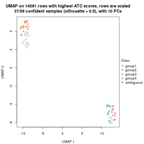
dimension_reduction(res, k = 5, method = "UMAP")
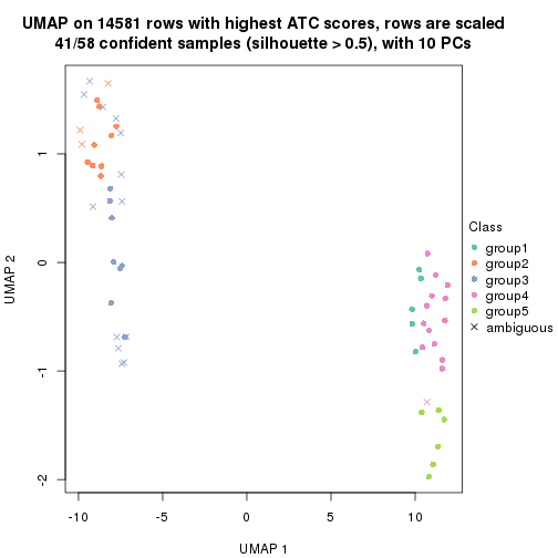
dimension_reduction(res, k = 6, method = "UMAP")
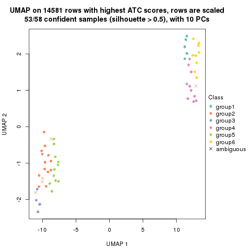
Following heatmap shows how subgroups are split when increasing k:
collect_classes(res)
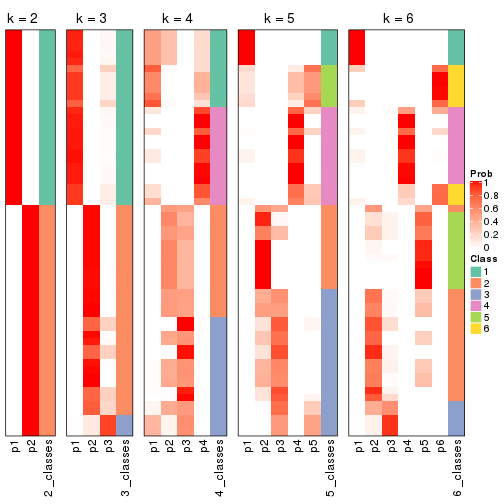
If matrix rows can be associated to genes, consider to use functional_enrichment(res,
...) to perform function enrichment for the signature genes. See this vignette for more detailed explanations.
The object with results only for a single top-value method and a single partition method can be extracted as:
res = res_list["ATC", "NMF"]
# you can also extract it by
# res = res_list["ATC:NMF"]
A summary of res and all the functions that can be applied to it:
res
#> A 'ConsensusPartition' object with k = 2, 3, 4, 5, 6.
#> On a matrix with 14581 rows and 58 columns.
#> Top rows (1000, 2000, 3000, 4000, 5000) are extracted by 'ATC' method.
#> Subgroups are detected by 'NMF' method.
#> Performed in total 1250 partitions by row resampling.
#> Best k for subgroups seems to be 4.
#>
#> Following methods can be applied to this 'ConsensusPartition' object:
#> [1] "cola_report" "collect_classes" "collect_plots"
#> [4] "collect_stats" "colnames" "compare_signatures"
#> [7] "consensus_heatmap" "dimension_reduction" "functional_enrichment"
#> [10] "get_anno_col" "get_anno" "get_classes"
#> [13] "get_consensus" "get_matrix" "get_membership"
#> [16] "get_param" "get_signatures" "get_stats"
#> [19] "is_best_k" "is_stable_k" "membership_heatmap"
#> [22] "ncol" "nrow" "plot_ecdf"
#> [25] "rownames" "select_partition_number" "show"
#> [28] "suggest_best_k" "test_to_known_factors"
collect_plots() function collects all the plots made from res for all k (number of partitions)
into one single page to provide an easy and fast comparison between different k.
collect_plots(res)
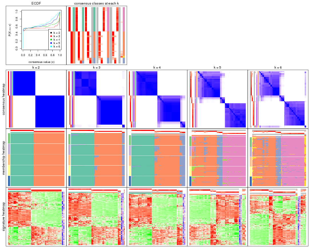
The plots are:
k and the heatmap of
predicted classes for each k.k.k.k.All the plots in panels can be made by individual functions and they are plotted later in this section.
select_partition_number() produces several plots showing different
statistics for choosing “optimized” k. There are following statistics:
k;k, the area increased is defined as \(A_k - A_{k-1}\).The detailed explanations of these statistics can be found in the cola vignette.
Generally speaking, lower PAC score, higher mean silhouette score or higher
concordance corresponds to better partition. Rand index and Jaccard index
measure how similar the current partition is compared to partition with k-1.
If they are too similar, we won't accept k is better than k-1.
select_partition_number(res)
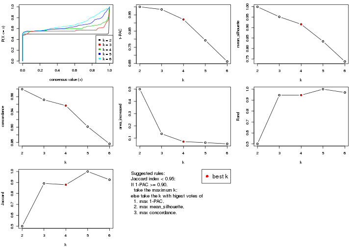
The numeric values for all these statistics can be obtained by get_stats().
get_stats(res)
#> k 1-PAC mean_silhouette concordance area_increased Rand Jaccard
#> 2 2 1.000 0.999 1.000 0.4997 0.501 0.501
#> 3 3 0.984 0.952 0.972 0.1355 0.946 0.891
#> 4 4 0.922 0.916 0.957 0.0718 0.946 0.880
#> 5 5 0.793 0.834 0.901 0.0635 1.000 1.000
#> 6 6 0.661 0.738 0.856 0.0535 0.970 0.925
suggest_best_k() suggests the best \(k\) based on these statistics. The rules are as follows:
suggest_best_k(res)
#> [1] 4
#> attr(,"optional")
#> [1] 2 3
There is also optional best \(k\) = 2 3 that is worth to check.
Following shows the table of the partitions (You need to click the show/hide
code output link to see it). The membership matrix (columns with name p*)
is inferred by
clue::cl_consensus()
function with the SE method. Basically the value in the membership matrix
represents the probability to belong to a certain group. The finall class
label for an item is determined with the group with highest probability it
belongs to.
In get_classes() function, the entropy is calculated from the membership
matrix and the silhouette score is calculated from the consensus matrix.
cbind(get_classes(res, k = 2), get_membership(res, k = 2))
#> class entropy silhouette p1 p2
#> ERR789082 2 0.000 0.999 0.00 1.00
#> ERR789083 2 0.000 0.999 0.00 1.00
#> ERR789191 2 0.000 0.999 0.00 1.00
#> ERR789192 2 0.000 0.999 0.00 1.00
#> ERR789213 1 0.000 1.000 1.00 0.00
#> ERR789385 1 0.000 1.000 1.00 0.00
#> ERR789393 1 0.000 1.000 1.00 0.00
#> ERR789394 1 0.000 1.000 1.00 0.00
#> ERR789193 2 0.000 0.999 0.00 1.00
#> ERR789194 2 0.000 0.999 0.00 1.00
#> ERR789195 2 0.000 0.999 0.00 1.00
#> ERR789196 2 0.000 0.999 0.00 1.00
#> ERR789388 1 0.000 1.000 1.00 0.00
#> ERR789197 2 0.000 0.999 0.00 1.00
#> ERR789198 2 0.000 0.999 0.00 1.00
#> ERR789214 1 0.000 1.000 1.00 0.00
#> ERR789397 1 0.000 1.000 1.00 0.00
#> ERR789398 1 0.000 1.000 1.00 0.00
#> ERR789199 2 0.000 0.999 0.00 1.00
#> ERR789200 2 0.000 0.999 0.00 1.00
#> ERR789201 2 0.000 0.999 0.00 1.00
#> ERR789202 2 0.000 0.999 0.00 1.00
#> ERR789215 1 0.000 1.000 1.00 0.00
#> ERR789203 2 0.000 0.999 0.00 1.00
#> ERR789204 2 0.000 0.999 0.00 1.00
#> ERR789383 1 0.000 1.000 1.00 0.00
#> ERR789205 2 0.000 0.999 0.00 1.00
#> ERR789206 2 0.000 0.999 0.00 1.00
#> ERR789399 1 0.000 1.000 1.00 0.00
#> ERR789400 1 0.000 1.000 1.00 0.00
#> ERR789207 2 0.000 0.999 0.00 1.00
#> ERR789208 2 0.000 0.999 0.00 1.00
#> ERR789209 2 0.000 0.999 0.00 1.00
#> ERR789210 2 0.000 0.999 0.00 1.00
#> ERR789211 2 0.000 0.999 0.00 1.00
#> ERR789212 2 0.000 0.999 0.00 1.00
#> ERR789386 1 0.000 1.000 1.00 0.00
#> ERR789076 2 0.000 0.999 0.00 1.00
#> ERR789077 2 0.000 0.999 0.00 1.00
#> ERR789384 1 0.000 1.000 1.00 0.00
#> ERR789078 2 0.000 0.999 0.00 1.00
#> ERR789079 2 0.000 0.999 0.00 1.00
#> ERR789216 1 0.000 1.000 1.00 0.00
#> ERR789080 2 0.000 0.999 0.00 1.00
#> ERR789387 1 0.000 1.000 1.00 0.00
#> ERR789081 2 0.000 0.999 0.00 1.00
#> ERR789064 2 0.000 0.999 0.00 1.00
#> ERR779485 2 0.141 0.980 0.02 0.98
#> ERR789065 2 0.000 0.999 0.00 1.00
#> ERR789401 1 0.000 1.000 1.00 0.00
#> ERR789402 1 0.000 1.000 1.00 0.00
#> ERR789403 1 0.000 1.000 1.00 0.00
#> ERR789389 1 0.000 1.000 1.00 0.00
#> ERR789395 1 0.000 1.000 1.00 0.00
#> ERR789396 1 0.000 1.000 1.00 0.00
#> ERR789390 1 0.000 1.000 1.00 0.00
#> ERR789391 1 0.000 1.000 1.00 0.00
#> ERR789392 1 0.000 1.000 1.00 0.00
cbind(get_classes(res, k = 3), get_membership(res, k = 3))
#> class entropy silhouette p1 p2 p3
#> ERR789082 2 0.0000 0.971 0.000 1.000 0.000
#> ERR789083 2 0.0000 0.971 0.000 1.000 0.000
#> ERR789191 2 0.0000 0.971 0.000 1.000 0.000
#> ERR789192 2 0.0000 0.971 0.000 1.000 0.000
#> ERR789213 1 0.3482 0.884 0.872 0.000 0.128
#> ERR789385 1 0.1529 0.964 0.960 0.000 0.040
#> ERR789393 1 0.1643 0.962 0.956 0.000 0.044
#> ERR789394 1 0.1753 0.960 0.952 0.000 0.048
#> ERR789193 3 0.3141 0.974 0.020 0.068 0.912
#> ERR789194 3 0.3234 0.972 0.020 0.072 0.908
#> ERR789195 2 0.1860 0.928 0.000 0.948 0.052
#> ERR789196 2 0.1753 0.932 0.000 0.952 0.048
#> ERR789388 1 0.0237 0.975 0.996 0.000 0.004
#> ERR789197 2 0.0000 0.971 0.000 1.000 0.000
#> ERR789198 2 0.0000 0.971 0.000 1.000 0.000
#> ERR789214 1 0.1753 0.960 0.952 0.000 0.048
#> ERR789397 1 0.1411 0.965 0.964 0.000 0.036
#> ERR789398 1 0.1529 0.964 0.960 0.000 0.040
#> ERR789199 2 0.0000 0.971 0.000 1.000 0.000
#> ERR789200 2 0.0000 0.971 0.000 1.000 0.000
#> ERR789201 2 0.0000 0.971 0.000 1.000 0.000
#> ERR789202 2 0.0000 0.971 0.000 1.000 0.000
#> ERR789215 1 0.0237 0.975 0.996 0.000 0.004
#> ERR789203 2 0.3619 0.837 0.000 0.864 0.136
#> ERR789204 2 0.3816 0.822 0.000 0.852 0.148
#> ERR789383 1 0.0892 0.971 0.980 0.000 0.020
#> ERR789205 2 0.0000 0.971 0.000 1.000 0.000
#> ERR789206 2 0.0000 0.971 0.000 1.000 0.000
#> ERR789399 1 0.0000 0.975 1.000 0.000 0.000
#> ERR789400 1 0.0000 0.975 1.000 0.000 0.000
#> ERR789207 2 0.0000 0.971 0.000 1.000 0.000
#> ERR789208 2 0.0000 0.971 0.000 1.000 0.000
#> ERR789209 2 0.0000 0.971 0.000 1.000 0.000
#> ERR789210 2 0.0000 0.971 0.000 1.000 0.000
#> ERR789211 2 0.0000 0.971 0.000 1.000 0.000
#> ERR789212 2 0.0000 0.971 0.000 1.000 0.000
#> ERR789386 1 0.0592 0.973 0.988 0.000 0.012
#> ERR789076 2 0.0000 0.971 0.000 1.000 0.000
#> ERR789077 2 0.0000 0.971 0.000 1.000 0.000
#> ERR789384 1 0.0747 0.972 0.984 0.000 0.016
#> ERR789078 2 0.0000 0.971 0.000 1.000 0.000
#> ERR789079 2 0.0000 0.971 0.000 1.000 0.000
#> ERR789216 1 0.0000 0.975 1.000 0.000 0.000
#> ERR789080 2 0.0000 0.971 0.000 1.000 0.000
#> ERR789387 1 0.0892 0.971 0.980 0.000 0.020
#> ERR789081 2 0.0000 0.971 0.000 1.000 0.000
#> ERR789064 2 0.0000 0.971 0.000 1.000 0.000
#> ERR779485 3 0.2176 0.956 0.020 0.032 0.948
#> ERR789065 2 0.6095 0.338 0.000 0.608 0.392
#> ERR789401 1 0.0892 0.971 0.980 0.000 0.020
#> ERR789402 1 0.0892 0.971 0.980 0.000 0.020
#> ERR789403 1 0.0892 0.971 0.980 0.000 0.020
#> ERR789389 1 0.0892 0.971 0.980 0.000 0.020
#> ERR789395 1 0.0892 0.971 0.980 0.000 0.020
#> ERR789396 1 0.0892 0.971 0.980 0.000 0.020
#> ERR789390 1 0.0000 0.975 1.000 0.000 0.000
#> ERR789391 1 0.0000 0.975 1.000 0.000 0.000
#> ERR789392 1 0.1753 0.960 0.952 0.000 0.048
cbind(get_classes(res, k = 4), get_membership(res, k = 4))
#> class entropy silhouette p1 p2 p3 p4
#> ERR789082 2 0.0188 0.944 0.000 0.996 0.004 NA
#> ERR789083 2 0.0188 0.944 0.000 0.996 0.004 NA
#> ERR789191 2 0.0188 0.944 0.000 0.996 0.004 NA
#> ERR789192 2 0.0188 0.944 0.000 0.996 0.004 NA
#> ERR789213 1 0.0376 0.980 0.992 0.000 0.004 NA
#> ERR789385 1 0.0188 0.981 0.996 0.000 0.000 NA
#> ERR789393 1 0.0188 0.981 0.996 0.000 0.000 NA
#> ERR789394 1 0.0188 0.981 0.996 0.000 0.000 NA
#> ERR789193 3 0.0657 0.858 0.000 0.012 0.984 NA
#> ERR789194 3 0.0524 0.857 0.000 0.008 0.988 NA
#> ERR789195 2 0.4222 0.611 0.000 0.728 0.272 NA
#> ERR789196 2 0.4454 0.536 0.000 0.692 0.308 NA
#> ERR789388 1 0.0188 0.981 0.996 0.000 0.000 NA
#> ERR789197 2 0.0188 0.944 0.000 0.996 0.004 NA
#> ERR789198 2 0.0188 0.944 0.000 0.996 0.004 NA
#> ERR789214 1 0.0188 0.981 0.996 0.000 0.000 NA
#> ERR789397 1 0.0336 0.980 0.992 0.000 0.000 NA
#> ERR789398 1 0.0336 0.980 0.992 0.000 0.000 NA
#> ERR789199 2 0.0188 0.944 0.000 0.996 0.004 NA
#> ERR789200 2 0.0188 0.944 0.000 0.996 0.004 NA
#> ERR789201 2 0.0188 0.944 0.000 0.996 0.004 NA
#> ERR789202 2 0.0188 0.944 0.000 0.996 0.004 NA
#> ERR789215 1 0.0000 0.981 1.000 0.000 0.000 NA
#> ERR789203 3 0.4277 0.691 0.000 0.280 0.720 NA
#> ERR789204 3 0.4277 0.691 0.000 0.280 0.720 NA
#> ERR789383 1 0.1118 0.968 0.964 0.000 0.000 NA
#> ERR789205 2 0.2216 0.869 0.000 0.908 0.092 NA
#> ERR789206 2 0.2814 0.824 0.000 0.868 0.132 NA
#> ERR789399 1 0.0188 0.981 0.996 0.000 0.000 NA
#> ERR789400 1 0.0188 0.981 0.996 0.000 0.000 NA
#> ERR789207 2 0.0000 0.944 0.000 1.000 0.000 NA
#> ERR789208 2 0.0000 0.944 0.000 1.000 0.000 NA
#> ERR789209 2 0.0188 0.943 0.000 0.996 0.004 NA
#> ERR789210 2 0.0000 0.944 0.000 1.000 0.000 NA
#> ERR789211 2 0.0000 0.944 0.000 1.000 0.000 NA
#> ERR789212 2 0.0000 0.944 0.000 1.000 0.000 NA
#> ERR789386 1 0.0707 0.977 0.980 0.000 0.000 NA
#> ERR789076 2 0.4770 0.565 0.000 0.700 0.288 NA
#> ERR789077 2 0.0000 0.944 0.000 1.000 0.000 NA
#> ERR789384 1 0.0469 0.981 0.988 0.000 0.000 NA
#> ERR789078 2 0.0188 0.942 0.000 0.996 0.000 NA
#> ERR789079 2 0.0469 0.937 0.000 0.988 0.000 NA
#> ERR789216 1 0.1474 0.961 0.948 0.000 0.000 NA
#> ERR789080 2 0.2053 0.884 0.000 0.924 0.004 NA
#> ERR789387 1 0.3610 0.816 0.800 0.000 0.000 NA
#> ERR789081 2 0.1118 0.920 0.000 0.964 0.000 NA
#> ERR789064 2 0.0000 0.944 0.000 1.000 0.000 NA
#> ERR779485 3 0.0376 0.853 0.000 0.004 0.992 NA
#> ERR789065 3 0.2216 0.846 0.000 0.092 0.908 NA
#> ERR789401 1 0.0469 0.979 0.988 0.000 0.000 NA
#> ERR789402 1 0.0707 0.977 0.980 0.000 0.000 NA
#> ERR789403 1 0.0336 0.980 0.992 0.000 0.000 NA
#> ERR789389 1 0.2216 0.926 0.908 0.000 0.000 NA
#> ERR789395 1 0.0707 0.977 0.980 0.000 0.000 NA
#> ERR789396 1 0.0707 0.977 0.980 0.000 0.000 NA
#> ERR789390 1 0.0188 0.981 0.996 0.000 0.000 NA
#> ERR789391 1 0.0188 0.981 0.996 0.000 0.000 NA
#> ERR789392 1 0.0188 0.981 0.996 0.000 0.000 NA
cbind(get_classes(res, k = 5), get_membership(res, k = 5))
#> class entropy silhouette p1 p2 p3 p4 p5
#> ERR789082 2 0.0162 0.871 NA 0.996 0.004 0.000 0.000
#> ERR789083 2 0.0162 0.871 NA 0.996 0.004 0.000 0.000
#> ERR789191 2 0.0162 0.871 NA 0.996 0.004 0.000 0.000
#> ERR789192 2 0.0162 0.871 NA 0.996 0.004 0.000 0.000
#> ERR789213 4 0.3635 0.815 NA 0.000 0.004 0.748 0.248
#> ERR789385 4 0.3109 0.855 NA 0.000 0.000 0.800 0.200
#> ERR789393 4 0.2891 0.870 NA 0.000 0.000 0.824 0.176
#> ERR789394 4 0.2966 0.864 NA 0.000 0.000 0.816 0.184
#> ERR789193 3 0.0510 0.856 NA 0.000 0.984 0.000 0.016
#> ERR789194 3 0.0510 0.856 NA 0.000 0.984 0.000 0.016
#> ERR789195 2 0.4060 0.408 NA 0.640 0.360 0.000 0.000
#> ERR789196 2 0.4114 0.364 NA 0.624 0.376 0.000 0.000
#> ERR789388 4 0.0510 0.942 NA 0.000 0.000 0.984 0.016
#> ERR789197 2 0.0290 0.871 NA 0.992 0.008 0.000 0.000
#> ERR789198 2 0.0290 0.871 NA 0.992 0.008 0.000 0.000
#> ERR789214 4 0.1197 0.938 NA 0.000 0.000 0.952 0.048
#> ERR789397 4 0.0703 0.941 NA 0.000 0.000 0.976 0.024
#> ERR789398 4 0.0703 0.941 NA 0.000 0.000 0.976 0.024
#> ERR789199 2 0.0162 0.871 NA 0.996 0.004 0.000 0.000
#> ERR789200 2 0.0162 0.871 NA 0.996 0.004 0.000 0.000
#> ERR789201 2 0.0932 0.867 NA 0.972 0.020 0.000 0.004
#> ERR789202 2 0.0932 0.867 NA 0.972 0.020 0.000 0.004
#> ERR789215 4 0.0794 0.943 NA 0.000 0.000 0.972 0.028
#> ERR789203 3 0.4244 0.654 NA 0.268 0.712 0.000 0.004
#> ERR789204 3 0.4314 0.632 NA 0.280 0.700 0.000 0.004
#> ERR789383 4 0.1444 0.934 NA 0.000 0.000 0.948 0.040
#> ERR789205 2 0.2833 0.778 NA 0.852 0.140 0.000 0.004
#> ERR789206 2 0.3167 0.739 NA 0.820 0.172 0.000 0.004
#> ERR789399 4 0.0510 0.941 NA 0.000 0.000 0.984 0.016
#> ERR789400 4 0.0510 0.941 NA 0.000 0.000 0.984 0.016
#> ERR789207 2 0.1365 0.866 NA 0.952 0.004 0.000 0.004
#> ERR789208 2 0.1365 0.866 NA 0.952 0.004 0.000 0.004
#> ERR789209 2 0.2284 0.856 NA 0.912 0.028 0.000 0.004
#> ERR789210 2 0.2125 0.858 NA 0.920 0.024 0.000 0.004
#> ERR789211 2 0.1644 0.862 NA 0.940 0.008 0.000 0.004
#> ERR789212 2 0.1644 0.862 NA 0.940 0.008 0.000 0.004
#> ERR789386 4 0.1282 0.941 NA 0.000 0.000 0.952 0.044
#> ERR789076 2 0.6109 0.300 NA 0.532 0.320 0.000 0.000
#> ERR789077 2 0.1478 0.856 NA 0.936 0.000 0.000 0.000
#> ERR789384 4 0.1764 0.933 NA 0.000 0.000 0.928 0.064
#> ERR789078 2 0.1544 0.854 NA 0.932 0.000 0.000 0.000
#> ERR789079 2 0.2852 0.777 NA 0.828 0.000 0.000 0.000
#> ERR789216 4 0.2359 0.926 NA 0.000 0.000 0.904 0.060
#> ERR789080 2 0.4306 0.353 NA 0.508 0.000 0.000 0.000
#> ERR789387 4 0.3521 0.858 NA 0.000 0.000 0.820 0.040
#> ERR789081 2 0.4074 0.557 NA 0.636 0.000 0.000 0.000
#> ERR789064 2 0.0880 0.867 NA 0.968 0.000 0.000 0.000
#> ERR779485 3 0.0451 0.853 NA 0.000 0.988 0.000 0.008
#> ERR789065 3 0.1568 0.849 NA 0.036 0.944 0.000 0.000
#> ERR789401 4 0.0671 0.942 NA 0.000 0.000 0.980 0.016
#> ERR789402 4 0.0992 0.939 NA 0.000 0.000 0.968 0.024
#> ERR789403 4 0.0566 0.942 NA 0.000 0.000 0.984 0.012
#> ERR789389 4 0.2077 0.926 NA 0.000 0.000 0.920 0.040
#> ERR789395 4 0.0898 0.939 NA 0.000 0.000 0.972 0.020
#> ERR789396 4 0.0955 0.939 NA 0.000 0.000 0.968 0.028
#> ERR789390 4 0.0290 0.942 NA 0.000 0.000 0.992 0.008
#> ERR789391 4 0.0162 0.942 NA 0.000 0.000 0.996 0.004
#> ERR789392 4 0.2966 0.864 NA 0.000 0.000 0.816 0.184
cbind(get_classes(res, k = 6), get_membership(res, k = 6))
#> class entropy silhouette p1 p2 p3 p4 p5 p6
#> ERR789082 2 0.0146 0.7706 NA 0.996 0.000 0.000 NA 0.004
#> ERR789083 2 0.0146 0.7706 NA 0.996 0.000 0.000 NA 0.004
#> ERR789191 2 0.0146 0.7706 NA 0.996 0.000 0.000 NA 0.004
#> ERR789192 2 0.0146 0.7706 NA 0.996 0.000 0.000 NA 0.004
#> ERR789213 4 0.4134 0.7316 NA 0.000 0.016 0.640 NA 0.000
#> ERR789385 4 0.3895 0.7821 NA 0.000 0.004 0.696 NA 0.000
#> ERR789393 4 0.3470 0.8275 NA 0.000 0.000 0.772 NA 0.000
#> ERR789394 4 0.3500 0.8245 NA 0.000 0.000 0.768 NA 0.000
#> ERR789193 3 0.0976 0.7386 NA 0.008 0.968 0.000 NA 0.000
#> ERR789194 3 0.1167 0.7382 NA 0.008 0.960 0.000 NA 0.000
#> ERR789195 2 0.3942 0.3435 NA 0.624 0.368 0.000 NA 0.004
#> ERR789196 2 0.4041 0.2306 NA 0.584 0.408 0.000 NA 0.004
#> ERR789388 4 0.2070 0.9013 NA 0.000 0.000 0.896 NA 0.000
#> ERR789197 2 0.0000 0.7710 NA 1.000 0.000 0.000 NA 0.000
#> ERR789198 2 0.0000 0.7710 NA 1.000 0.000 0.000 NA 0.000
#> ERR789214 4 0.2692 0.8884 NA 0.000 0.000 0.840 NA 0.000
#> ERR789397 4 0.1866 0.9021 NA 0.000 0.000 0.908 NA 0.000
#> ERR789398 4 0.1753 0.9026 NA 0.000 0.000 0.912 NA 0.000
#> ERR789199 2 0.0000 0.7710 NA 1.000 0.000 0.000 NA 0.000
#> ERR789200 2 0.0000 0.7710 NA 1.000 0.000 0.000 NA 0.000
#> ERR789201 2 0.2325 0.7364 NA 0.892 0.048 0.000 NA 0.000
#> ERR789202 2 0.2328 0.7350 NA 0.892 0.052 0.000 NA 0.000
#> ERR789215 4 0.2237 0.9020 NA 0.000 0.000 0.896 NA 0.004
#> ERR789203 3 0.4637 0.4755 NA 0.308 0.628 0.000 NA 0.000
#> ERR789204 3 0.4844 0.4605 NA 0.312 0.608 0.000 NA 0.000
#> ERR789383 4 0.1578 0.8981 NA 0.000 0.000 0.936 NA 0.004
#> ERR789205 2 0.3572 0.5988 NA 0.764 0.204 0.000 NA 0.000
#> ERR789206 2 0.3566 0.5802 NA 0.752 0.224 0.000 NA 0.000
#> ERR789399 4 0.1003 0.9034 NA 0.000 0.000 0.964 NA 0.000
#> ERR789400 4 0.1003 0.9034 NA 0.000 0.000 0.964 NA 0.000
#> ERR789207 2 0.2822 0.7211 NA 0.856 0.004 0.000 NA 0.032
#> ERR789208 2 0.2747 0.7232 NA 0.860 0.004 0.000 NA 0.028
#> ERR789209 2 0.3879 0.6849 NA 0.788 0.052 0.000 NA 0.020
#> ERR789210 2 0.3973 0.6821 NA 0.784 0.048 0.000 NA 0.028
#> ERR789211 2 0.3084 0.7085 NA 0.832 0.008 0.000 NA 0.024
#> ERR789212 2 0.3001 0.7110 NA 0.840 0.008 0.000 NA 0.024
#> ERR789386 4 0.2070 0.9007 NA 0.000 0.000 0.892 NA 0.000
#> ERR789076 2 0.6641 -0.1464 NA 0.456 0.296 0.000 NA 0.212
#> ERR789077 2 0.2655 0.6726 NA 0.848 0.000 0.000 NA 0.140
#> ERR789384 4 0.2442 0.8898 NA 0.000 0.000 0.852 NA 0.004
#> ERR789078 2 0.2833 0.6609 NA 0.836 0.000 0.000 NA 0.148
#> ERR789079 2 0.3706 -0.0126 NA 0.620 0.000 0.000 NA 0.380
#> ERR789216 4 0.3235 0.8799 NA 0.000 0.000 0.824 NA 0.032
#> ERR789080 6 0.2996 0.7764 NA 0.228 0.000 0.000 NA 0.772
#> ERR789387 4 0.4656 0.7361 NA 0.000 0.000 0.704 NA 0.212
#> ERR789081 6 0.3620 0.7662 NA 0.352 0.000 0.000 NA 0.648
#> ERR789064 2 0.1141 0.7535 NA 0.948 0.000 0.000 NA 0.052
#> ERR779485 3 0.0653 0.7357 NA 0.004 0.980 0.000 NA 0.000
#> ERR789065 3 0.1942 0.7252 NA 0.064 0.916 0.000 NA 0.012
#> ERR789401 4 0.0520 0.9037 NA 0.000 0.000 0.984 NA 0.000
#> ERR789402 4 0.0622 0.9035 NA 0.000 0.000 0.980 NA 0.000
#> ERR789403 4 0.0520 0.9037 NA 0.000 0.000 0.984 NA 0.000
#> ERR789389 4 0.1875 0.8989 NA 0.000 0.000 0.928 NA 0.020
#> ERR789395 4 0.0717 0.9028 NA 0.000 0.000 0.976 NA 0.000
#> ERR789396 4 0.0717 0.9028 NA 0.000 0.000 0.976 NA 0.000
#> ERR789390 4 0.0717 0.9059 NA 0.000 0.000 0.976 NA 0.000
#> ERR789391 4 0.0717 0.9059 NA 0.000 0.000 0.976 NA 0.000
#> ERR789392 4 0.3500 0.8245 NA 0.000 0.000 0.768 NA 0.000
Heatmaps for the consensus matrix. It visualizes the probability of two samples to be in a same group.
consensus_heatmap(res, k = 2)
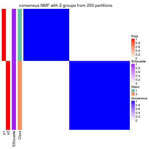
consensus_heatmap(res, k = 3)
consensus_heatmap(res, k = 4)
consensus_heatmap(res, k = 5)
consensus_heatmap(res, k = 6)
Heatmaps for the membership of samples in all partitions to see how consistent they are:
membership_heatmap(res, k = 2)

membership_heatmap(res, k = 3)

membership_heatmap(res, k = 4)
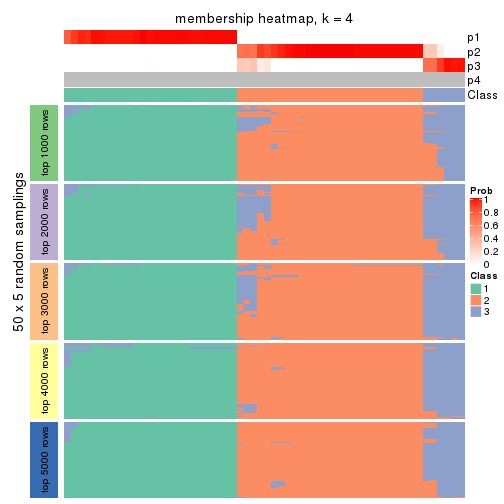
membership_heatmap(res, k = 5)
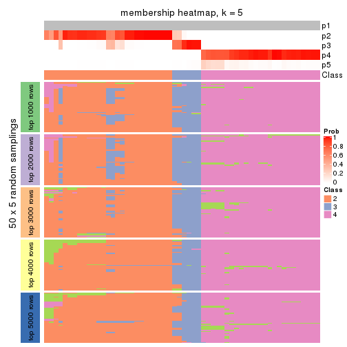
membership_heatmap(res, k = 6)
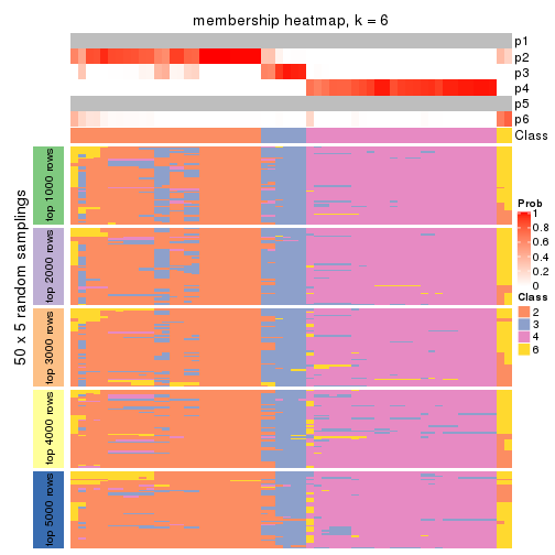
As soon as we have had the classes for columns, we can look for signatures which are significantly different between classes which can be candidate marks for certain classes. Following are the heatmaps for signatures.
Signature heatmaps where rows are scaled:
get_signatures(res, k = 2)

get_signatures(res, k = 3)
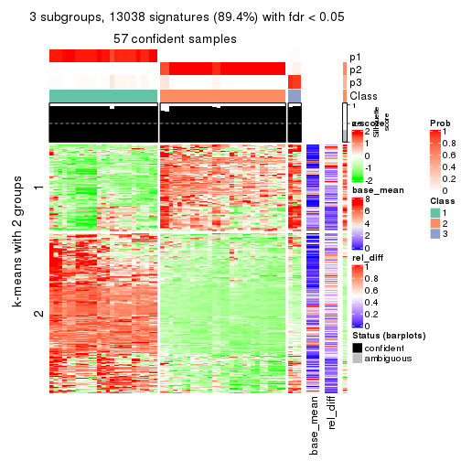
get_signatures(res, k = 4)
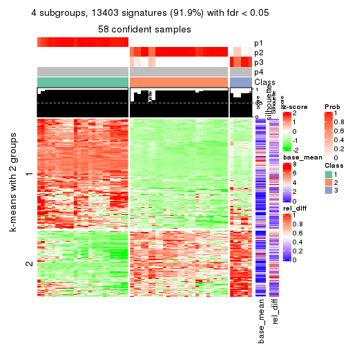
get_signatures(res, k = 5)
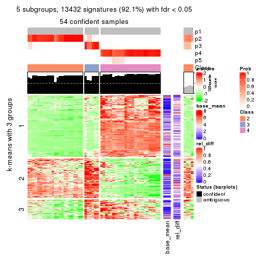
get_signatures(res, k = 6)
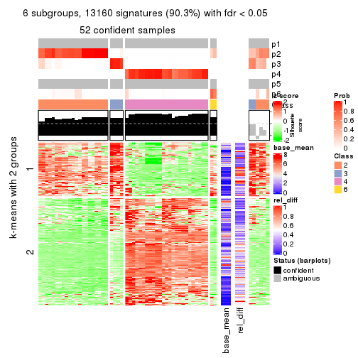
Signature heatmaps where rows are not scaled:
get_signatures(res, k = 2, scale_rows = FALSE)

get_signatures(res, k = 3, scale_rows = FALSE)
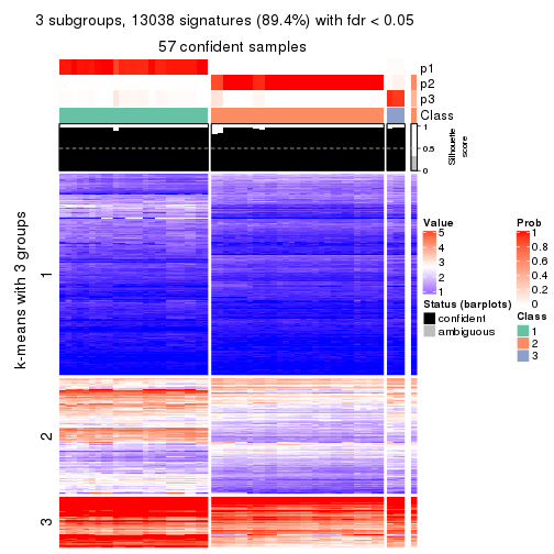
get_signatures(res, k = 4, scale_rows = FALSE)
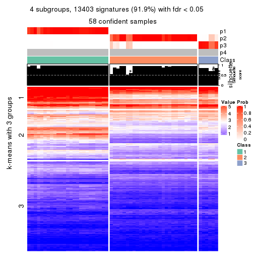
get_signatures(res, k = 5, scale_rows = FALSE)
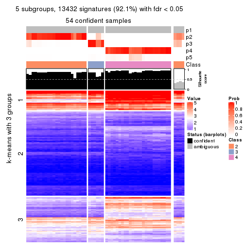
get_signatures(res, k = 6, scale_rows = FALSE)
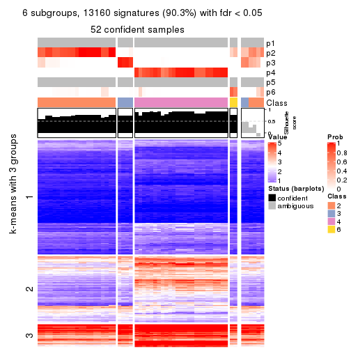
Compare the overlap of signatures from different k:
compare_signatures(res)
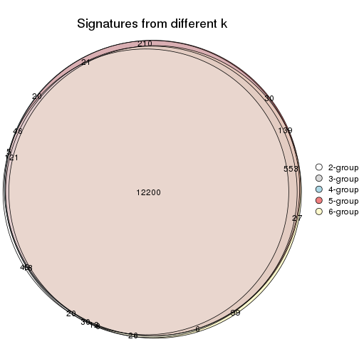
get_signature() returns a data frame invisibly. TO get the list of signatures, the function
call should be assigned to a variable explicitly. In following code, if plot argument is set
to FALSE, no heatmap is plotted while only the differential analysis is performed.
# code only for demonstration
tb = get_signature(res, k = ..., plot = FALSE)
An example of the output of tb is:
#> which_row fdr mean_1 mean_2 scaled_mean_1 scaled_mean_2 km
#> 1 38 0.042760348 8.373488 9.131774 -0.5533452 0.5164555 1
#> 2 40 0.018707592 7.106213 8.469186 -0.6173731 0.5762149 1
#> 3 55 0.019134737 10.221463 11.207825 -0.6159697 0.5749050 1
#> 4 59 0.006059896 5.921854 7.869574 -0.6899429 0.6439467 1
#> 5 60 0.018055526 8.928898 10.211722 -0.6204761 0.5791110 1
#> 6 98 0.009384629 15.714769 14.887706 0.6635654 -0.6193277 2
...
The columns in tb are:
which_row: row indices corresponding to the input matrix.fdr: FDR for the differential test. mean_x: The mean value in group x.scaled_mean_x: The mean value in group x after rows are scaled.km: Row groups if k-means clustering is applied to rows.UMAP plot which shows how samples are separated.
dimension_reduction(res, k = 2, method = "UMAP")
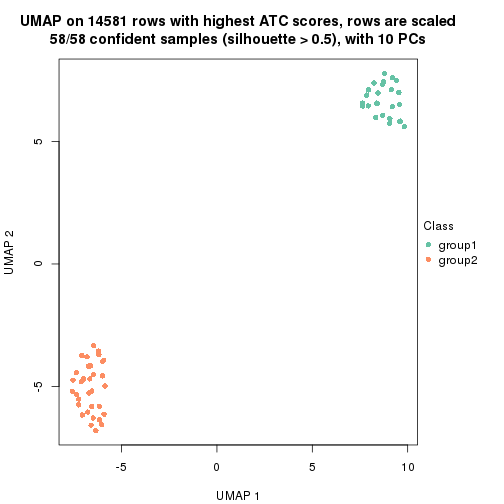
dimension_reduction(res, k = 3, method = "UMAP")
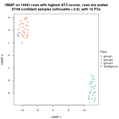
dimension_reduction(res, k = 4, method = "UMAP")
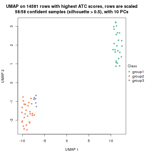
dimension_reduction(res, k = 5, method = "UMAP")
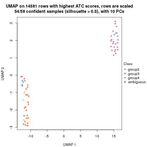
dimension_reduction(res, k = 6, method = "UMAP")
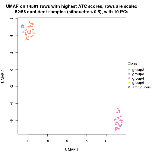
Following heatmap shows how subgroups are split when increasing k:
collect_classes(res)
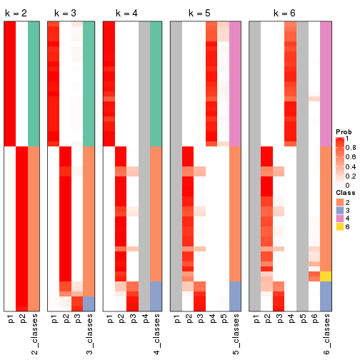
If matrix rows can be associated to genes, consider to use functional_enrichment(res,
...) to perform function enrichment for the signature genes. See this vignette for more detailed explanations.
sessionInfo()
#> R version 3.6.0 (2019-04-26)
#> Platform: x86_64-pc-linux-gnu (64-bit)
#> Running under: CentOS Linux 7 (Core)
#>
#> Matrix products: default
#> BLAS: /usr/lib64/libblas.so.3.4.2
#> LAPACK: /usr/lib64/liblapack.so.3.4.2
#>
#> locale:
#> [1] LC_CTYPE=en_GB.UTF-8 LC_NUMERIC=C LC_TIME=en_GB.UTF-8
#> [4] LC_COLLATE=en_GB.UTF-8 LC_MONETARY=en_GB.UTF-8 LC_MESSAGES=en_GB.UTF-8
#> [7] LC_PAPER=en_GB.UTF-8 LC_NAME=C LC_ADDRESS=C
#> [10] LC_TELEPHONE=C LC_MEASUREMENT=en_GB.UTF-8 LC_IDENTIFICATION=C
#>
#> attached base packages:
#> [1] grid stats graphics grDevices utils datasets methods base
#>
#> other attached packages:
#> [1] genefilter_1.66.0 ComplexHeatmap_2.3.1 markdown_1.1 knitr_1.26
#> [5] GetoptLong_0.1.7 cola_1.3.2
#>
#> loaded via a namespace (and not attached):
#> [1] circlize_0.4.8 shape_1.4.4 xfun_0.11 slam_0.1-46
#> [5] lattice_0.20-38 splines_3.6.0 colorspace_1.4-1 vctrs_0.2.0
#> [9] stats4_3.6.0 blob_1.2.0 XML_3.98-1.20 survival_2.44-1.1
#> [13] rlang_0.4.2 pillar_1.4.2 DBI_1.0.0 BiocGenerics_0.30.0
#> [17] bit64_0.9-7 RColorBrewer_1.1-2 matrixStats_0.55.0 stringr_1.4.0
#> [21] GlobalOptions_0.1.1 evaluate_0.14 memoise_1.1.0 Biobase_2.44.0
#> [25] IRanges_2.18.3 parallel_3.6.0 AnnotationDbi_1.46.1 highr_0.8
#> [29] Rcpp_1.0.3 xtable_1.8-4 backports_1.1.5 S4Vectors_0.22.1
#> [33] annotate_1.62.0 skmeans_0.2-11 bit_1.1-14 microbenchmark_1.4-7
#> [37] brew_1.0-6 impute_1.58.0 rjson_0.2.20 png_0.1-7
#> [41] digest_0.6.23 stringi_1.4.3 polyclip_1.10-0 clue_0.3-57
#> [45] tools_3.6.0 bitops_1.0-6 magrittr_1.5 eulerr_6.0.0
#> [49] RCurl_1.95-4.12 RSQLite_2.1.4 tibble_2.1.3 cluster_2.1.0
#> [53] crayon_1.3.4 pkgconfig_2.0.3 zeallot_0.1.0 Matrix_1.2-17
#> [57] xml2_1.2.2 httr_1.4.1 R6_2.4.1 mclust_5.4.5
#> [61] compiler_3.6.0