
Date: 2019-12-25 23:05:51 CET, cola version: 1.3.2
Document is loading...
All available functions which can be applied to this res_list object:
res_list
#> A 'ConsensusPartitionList' object with 24 methods.
#>   On a matrix with 14662 rows and 56 columns.
#>   Top rows are extracted by 'SD, CV, MAD, ATC' methods.
#>   Subgroups are detected by 'hclust, kmeans, skmeans, pam, mclust, NMF' method.
#>   Number of partitions are tried for k = 2, 3, 4, 5, 6.
#>   Performed in total 30000 partitions by row resampling.
#>
#> Following methods can be applied to this 'ConsensusPartitionList' object:
#>  [1] "cola_report"           "collect_classes"       "collect_plots"         "collect_stats"
#>  [5] "colnames"              "functional_enrichment" "get_anno_col"          "get_anno"
#>  [9] "get_classes"           "get_matrix"            "get_membership"        "get_stats"
#> [13] "is_best_k"             "is_stable_k"           "ncol"                  "nrow"
#> [17] "rownames"              "show"                  "suggest_best_k"        "test_to_known_factors"
#> [21] "top_rows_heatmap"      "top_rows_overlap"
#>
#> You can get result for a single method by, e.g. object["SD", "hclust"] or object["SD:hclust"]
#> or a subset of methods by object[c("SD", "CV")], c("hclust", "kmeans")]
The call of run_all_consensus_partition_methods() was:
#> run_all_consensus_partition_methods(data = mat, mc.cores = 4)
Dimension of the input matrix:
mat = get_matrix(res_list)
dim(mat)
#> [1] 14662 56
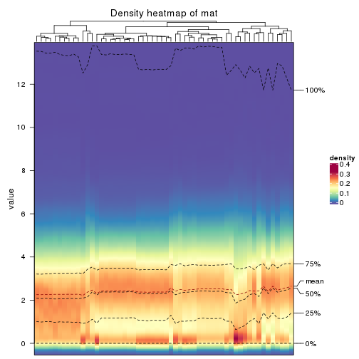
The density distribution for each sample is visualized as in one column in the following heatmap. The clustering is based on the distance which is the Kolmogorov-Smirnov statistic between two distributions.
library(ComplexHeatmap)
densityHeatmap(mat, ylab = "value", cluster_columns = TRUE, show_column_names = FALSE,
    mc.cores = 4)
Folowing table shows the best k (number of partitions) for each combination
of top-value methods and partition methods. Clicking on the method name in
the table goes to the section for a single combination of methods.
The cola vignette explains the definition of the metrics used for determining the best number of partitions.
suggest_best_k(res_list)
| The best k | 1-PAC | Mean silhouette | Concordance | Optional k | ||
|---|---|---|---|---|---|---|
| SD:pam | 6 | 1.000 | 0.951 | 0.981 | ** | 2,4,5 |
| CV:pam | 6 | 1.000 | 0.950 | 0.982 | ** | 2,4,5 |
| ATC:pam | 6 | 1.000 | 0.965 | 0.989 | ** | 2,3,4,5 |
| ATC:NMF | 2 | 1.000 | 0.993 | 0.997 | ** | |
| ATC:skmeans | 3 | 0.992 | 0.975 | 0.965 | ** | 2 |
| MAD:pam | 6 | 0.982 | 0.950 | 0.980 | ** | 2,4,5 |
| CV:hclust | 4 | 0.971 | 0.972 | 0.984 | ** | 3 |
| CV:mclust | 6 | 0.970 | 0.944 | 0.971 | ** | 3,4,5 |
| SD:hclust | 6 | 0.939 | 0.963 | 0.964 | * | 3 |
| ATC:hclust | 4 | 0.935 | 0.921 | 0.950 | * | |
| MAD:skmeans | 3 | 0.932 | 0.860 | 0.928 | * | 2 |
| SD:kmeans | 2 | 0.923 | 0.902 | 0.940 | * | |
| CV:skmeans | 6 | 0.919 | 0.847 | 0.893 | * | 2,3,4,5 |
| CV:NMF | 6 | 0.915 | 0.944 | 0.947 | * | 2,4,5 |
| SD:skmeans | 6 | 0.911 | 0.776 | 0.875 | * | 2,4,5 |
| SD:NMF | 6 | 0.907 | 0.877 | 0.929 | * | 2,4 |
| ATC:mclust | 6 | 0.906 | 0.840 | 0.928 | * | 2 |
| MAD:mclust | 6 | 0.904 | 0.903 | 0.937 | * | 2 |
| MAD:NMF | 5 | 0.902 | 0.897 | 0.933 | * | 2,4 |
| SD:mclust | 4 | 0.828 | 0.923 | 0.955 | ||
| MAD:hclust | 3 | 0.792 | 0.804 | 0.906 | ||
| MAD:kmeans | 2 | 0.642 | 0.894 | 0.921 | ||
| ATC:kmeans | 2 | 0.572 | 0.962 | 0.960 | ||
| CV:kmeans | 2 | 0.353 | 0.851 | 0.862 |
**: 1-PAC > 0.95, *: 1-PAC > 0.9
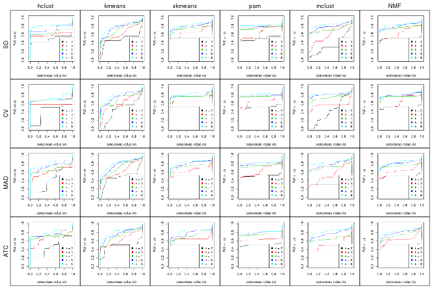
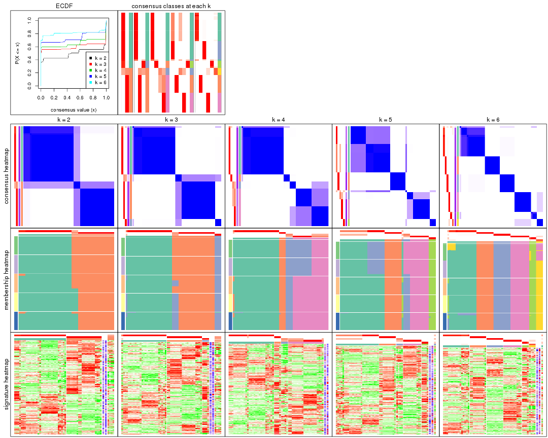
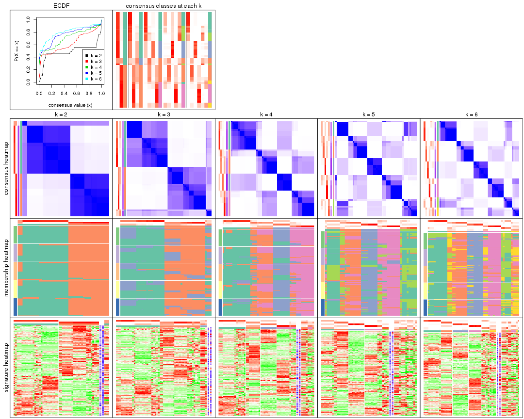
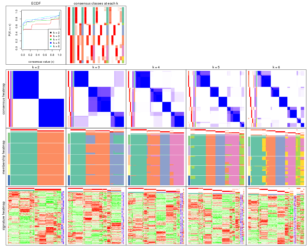
Cumulative distribution function curves of consensus matrix for all methods.
collect_plots(res_list, fun = plot_ecdf)
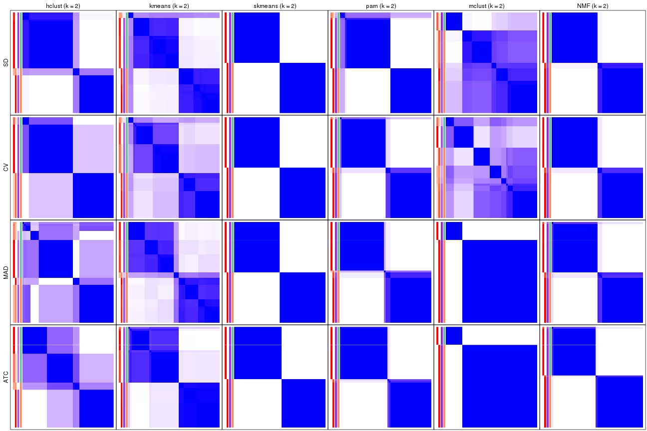
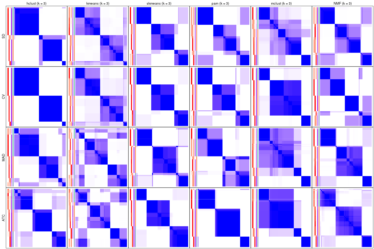
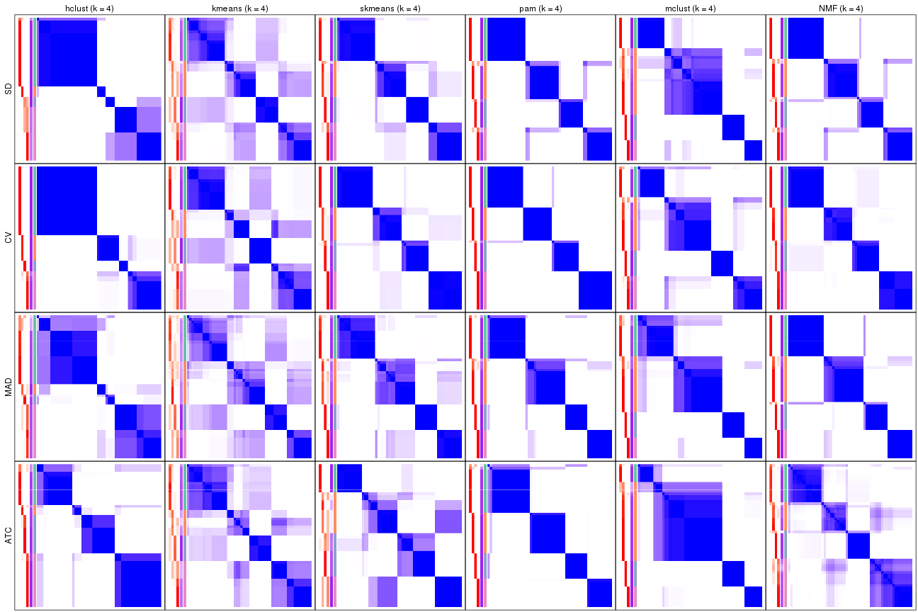
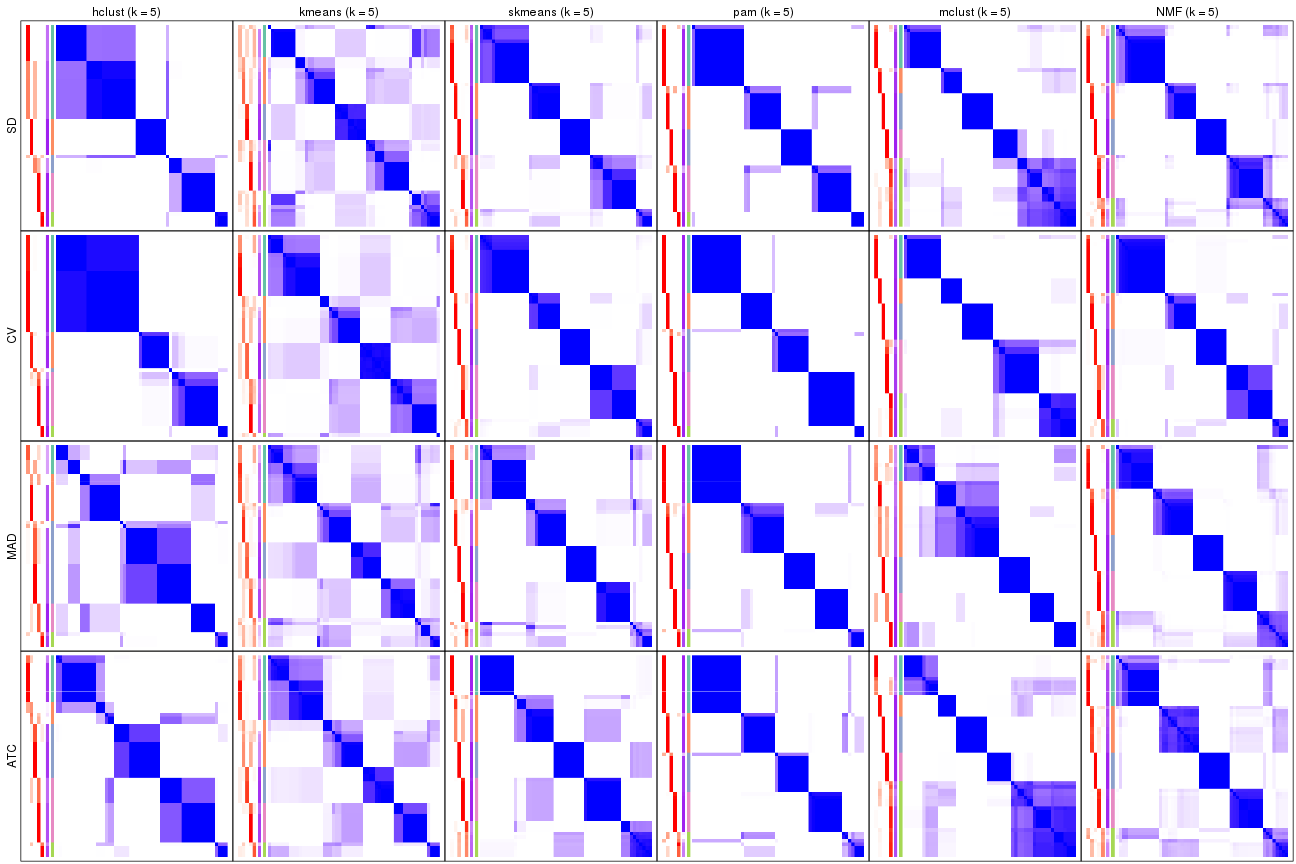
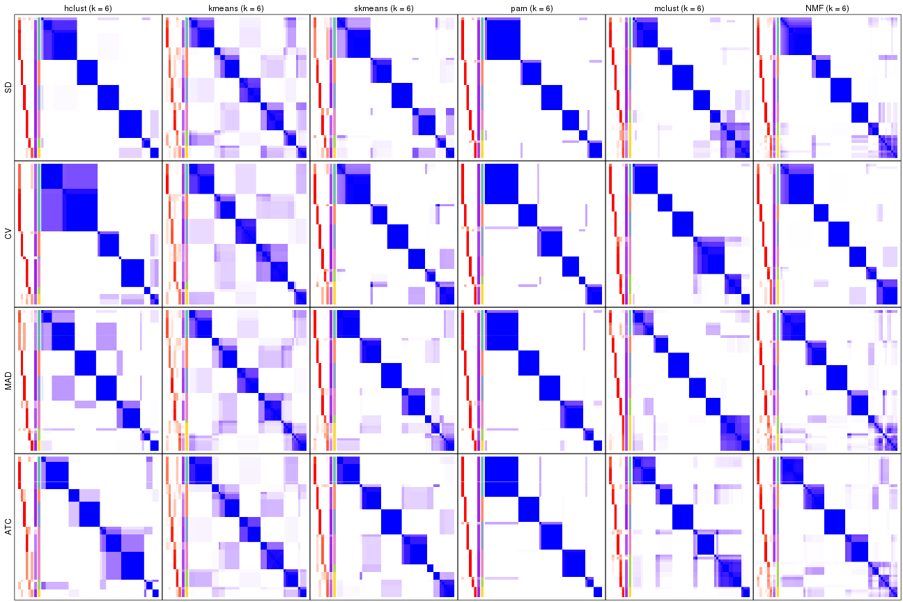
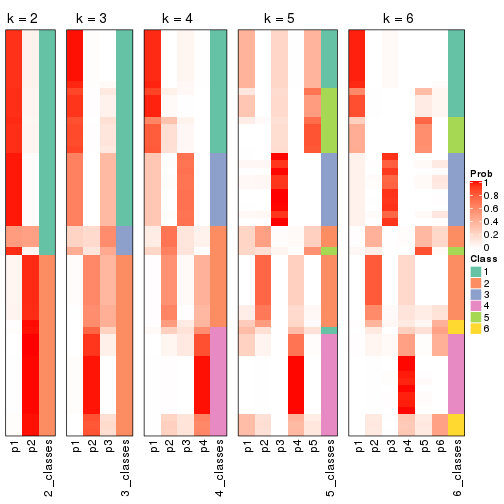
Consensus heatmaps for all methods. (What is a consensus heatmap?)
collect_plots(res_list, k = 2, fun = consensus_heatmap, mc.cores = 4)
collect_plots(res_list, k = 3, fun = consensus_heatmap, mc.cores = 4)
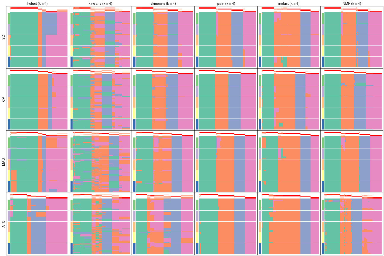
collect_plots(res_list, k = 4, fun = consensus_heatmap, mc.cores = 4)
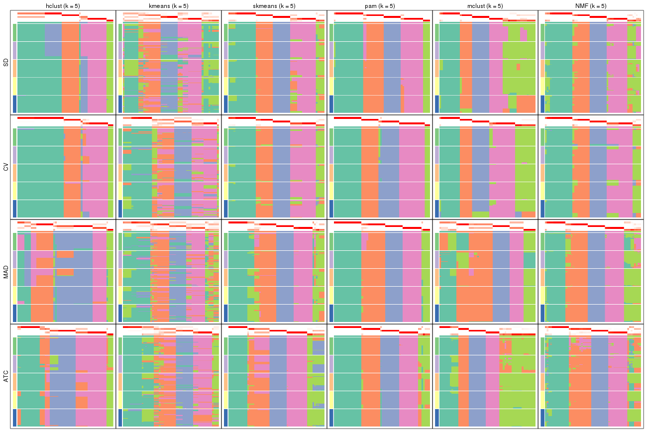
collect_plots(res_list, k = 5, fun = consensus_heatmap, mc.cores = 4)
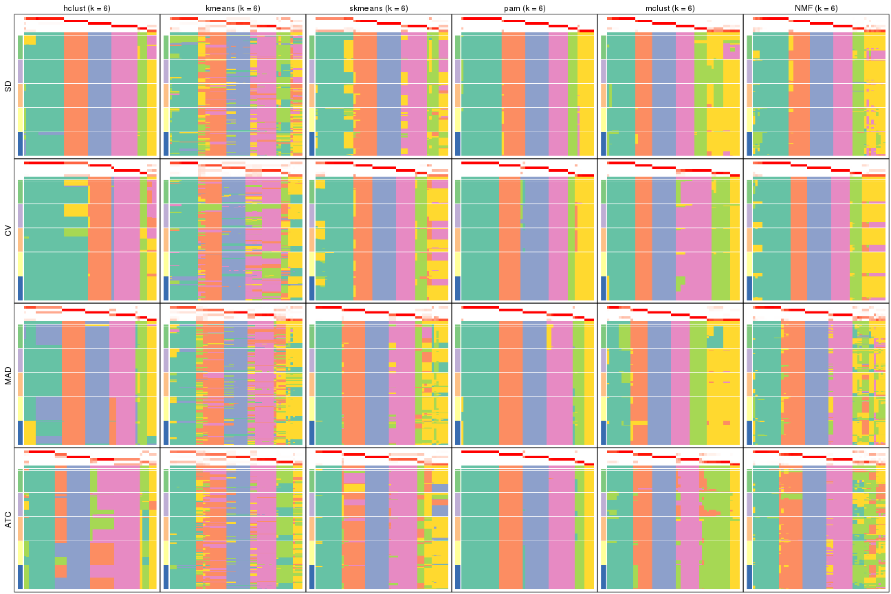
collect_plots(res_list, k = 6, fun = consensus_heatmap, mc.cores = 4)
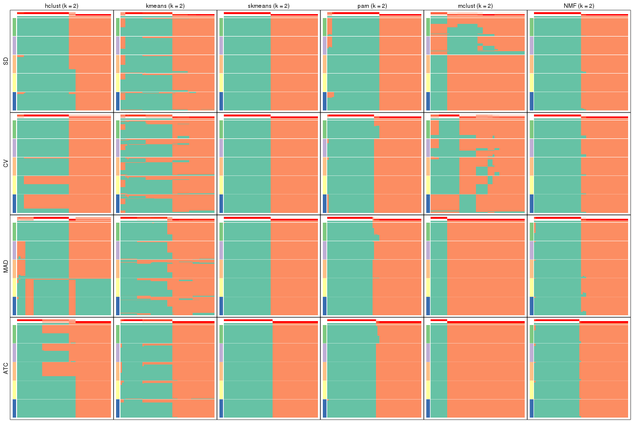
Membership heatmaps for all methods. (What is a membership heatmap?)
collect_plots(res_list, k = 2, fun = membership_heatmap, mc.cores = 4)
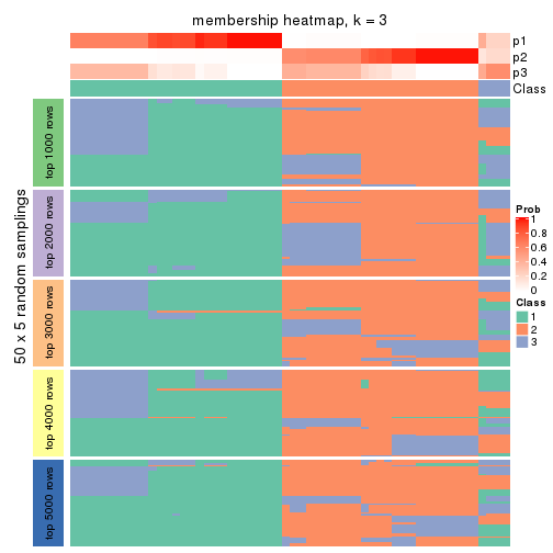
collect_plots(res_list, k = 3, fun = membership_heatmap, mc.cores = 4)

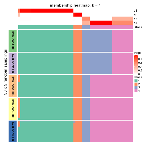
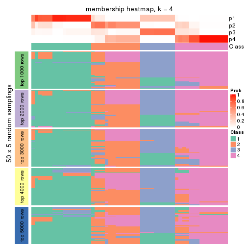
collect_plots(res_list, k = 4, fun = membership_heatmap, mc.cores = 4)
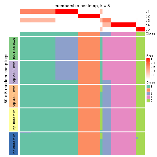
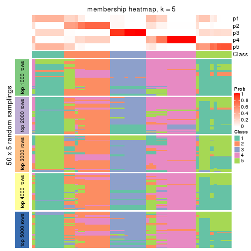
collect_plots(res_list, k = 5, fun = membership_heatmap, mc.cores = 4)
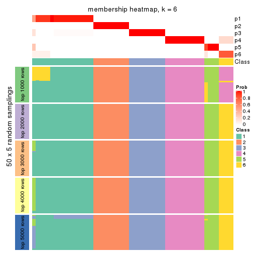
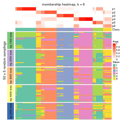
collect_plots(res_list, k = 6, fun = membership_heatmap, mc.cores = 4)
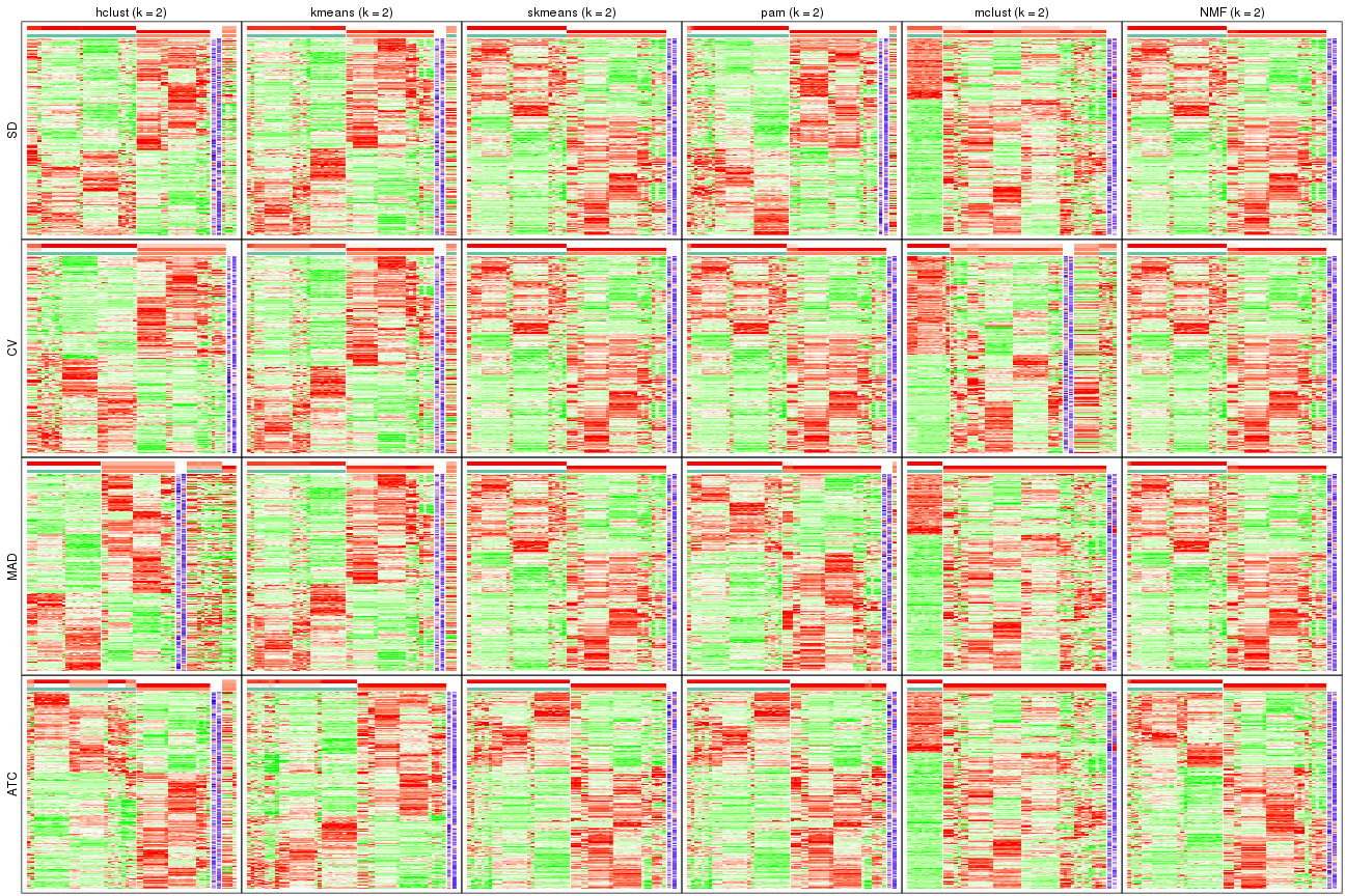
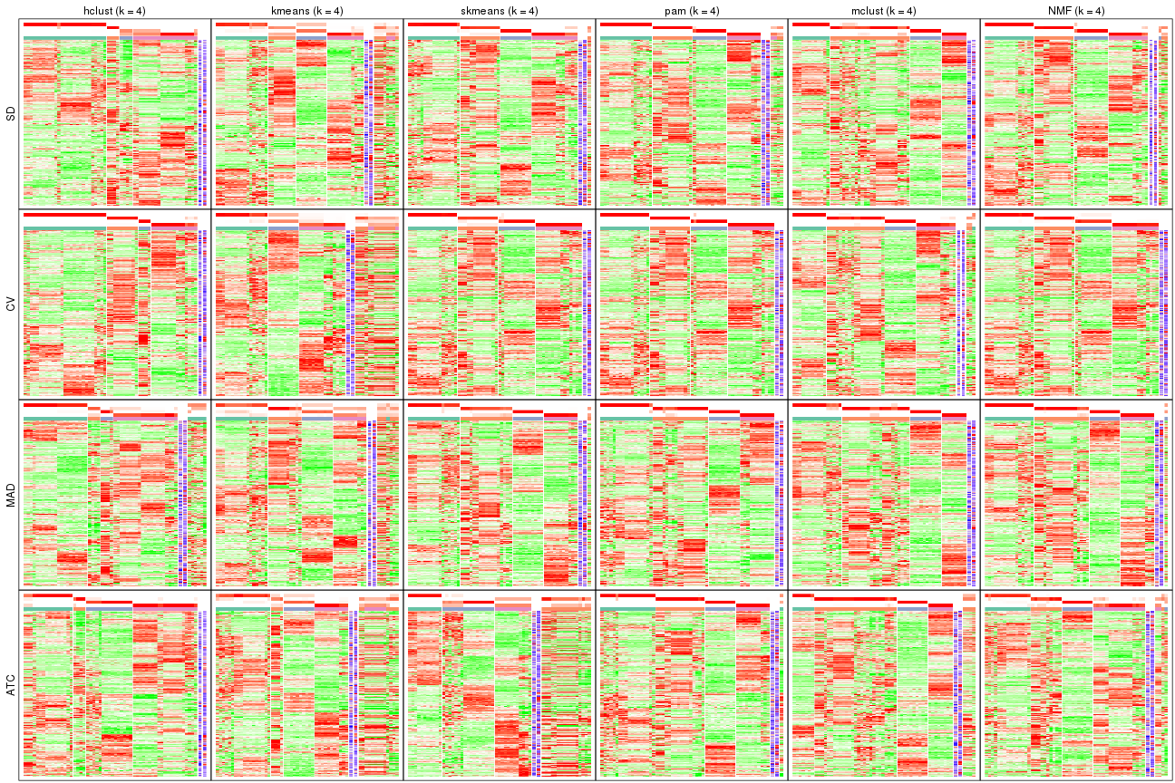
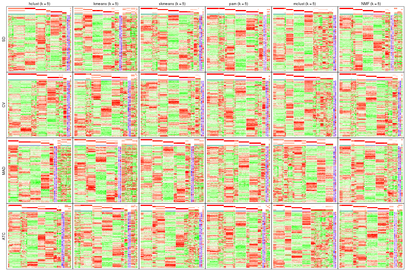
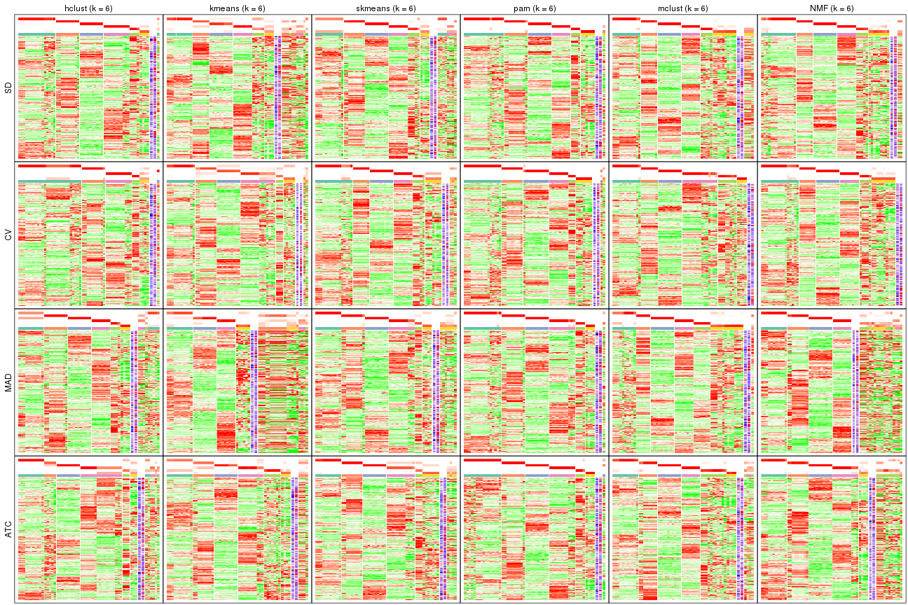
Signature heatmaps for all methods. (What is a signature heatmap?)
Note in following heatmaps, rows are scaled.
collect_plots(res_list, k = 2, fun = get_signatures, mc.cores = 4)
collect_plots(res_list, k = 3, fun = get_signatures, mc.cores = 4)

collect_plots(res_list, k = 4, fun = get_signatures, mc.cores = 4)
collect_plots(res_list, k = 5, fun = get_signatures, mc.cores = 4)
collect_plots(res_list, k = 6, fun = get_signatures, mc.cores = 4)
The statistics used for measuring the stability of consensus partitioning. (How are they defined?)
get_stats(res_list, k = 2)
#>             k 1-PAC mean_silhouette concordance area_increased  Rand Jaccard
#> SD:NMF      2 1.000           0.995       0.997          0.509 0.491   0.491
#> CV:NMF      2 1.000           0.989       0.995          0.509 0.491   0.491
#> MAD:NMF     2 1.000           0.984       0.992          0.509 0.491   0.491
#> ATC:NMF     2 1.000           0.993       0.997          0.509 0.492   0.492
#> SD:skmeans  2 1.000           1.000       1.000          0.510 0.491   0.491
#> CV:skmeans  2 1.000           1.000       1.000          0.510 0.491   0.491
#> MAD:skmeans 2 1.000           1.000       1.000          0.510 0.491   0.491
#> ATC:skmeans 2 1.000           1.000       1.000          0.509 0.492   0.492
#> SD:mclust   2 0.442           0.857       0.800          0.347 0.701   0.701
#> CV:mclust   2 0.214           0.694       0.810          0.417 0.569   0.569
#> MAD:mclust  2 1.000           1.000       1.000          0.299 0.701   0.701
#> ATC:mclust  2 1.000           1.000       1.000          0.299 0.701   0.701
#> SD:kmeans   2 0.923           0.902       0.940          0.491 0.497   0.497
#> CV:kmeans   2 0.353           0.851       0.863          0.450 0.497   0.497
#> MAD:kmeans  2 0.642           0.894       0.921          0.489 0.491   0.491
#> ATC:kmeans  2 0.572           0.962       0.960          0.487 0.497   0.497
#> SD:pam      2 1.000           0.952       0.980          0.506 0.497   0.497
#> CV:pam      2 0.962           0.973       0.988          0.509 0.491   0.491
#> MAD:pam     2 1.000           0.977       0.990          0.509 0.492   0.492
#> ATC:pam     2 1.000           0.989       0.995          0.508 0.492   0.492
#> SD:hclust   2 0.865           0.919       0.967          0.493 0.497   0.497
#> CV:hclust   2 0.492           0.959       0.880          0.413 0.497   0.497
#> MAD:hclust  2 0.425           0.684       0.779          0.418 0.497   0.497
#> ATC:hclust  2 0.544           0.738       0.875          0.458 0.497   0.497
get_stats(res_list, k = 3)
#>             k 1-PAC mean_silhouette concordance area_increased  Rand Jaccard
#> SD:NMF      3 0.734           0.851       0.768          0.253 0.875   0.746
#> CV:NMF      3 0.748           0.771       0.820          0.277 0.847   0.694
#> MAD:NMF     3 0.766           0.925       0.916          0.234 0.854   0.713
#> ATC:NMF     3 0.721           0.920       0.913          0.251 0.857   0.715
#> SD:skmeans  3 0.741           0.905       0.908          0.286 0.803   0.617
#> CV:skmeans  3 1.000           0.979       0.976          0.292 0.803   0.617
#> MAD:skmeans 3 0.932           0.860       0.928          0.265 0.831   0.665
#> ATC:skmeans 3 0.992           0.975       0.965          0.267 0.816   0.642
#> SD:mclust   3 0.546           0.715       0.845          0.774 0.659   0.514
#> CV:mclust   3 1.000           0.970       0.976          0.357 0.679   0.516
#> MAD:mclust  3 0.522           0.799       0.841          0.828 0.803   0.719
#> ATC:mclust  3 0.667           0.923       0.930          0.703 0.803   0.719
#> SD:kmeans   3 0.619           0.679       0.772          0.274 0.930   0.859
#> CV:kmeans   3 0.610           0.727       0.803          0.354 0.930   0.859
#> MAD:kmeans  3 0.618           0.574       0.737          0.292 0.842   0.687
#> ATC:kmeans  3 0.630           0.503       0.705          0.307 0.848   0.694
#> SD:pam      3 0.730           0.786       0.780          0.283 0.845   0.689
#> CV:pam      3 0.737           0.918       0.927          0.288 0.803   0.617
#> MAD:pam     3 0.687           0.714       0.774          0.249 0.864   0.723
#> ATC:pam     3 1.000           0.970       0.988          0.250 0.877   0.749
#> SD:hclust   3 0.913           0.900       0.960          0.213 0.930   0.859
#> CV:hclust   3 1.000           1.000       1.000          0.390 0.930   0.859
#> MAD:hclust  3 0.792           0.804       0.906          0.467 0.865   0.734
#> ATC:hclust  3 0.694           0.905       0.912          0.406 0.748   0.532
get_stats(res_list, k = 4)
#>             k 1-PAC mean_silhouette concordance area_increased  Rand Jaccard
#> SD:NMF      4 0.946           0.901       0.962         0.1856 0.873   0.654
#> CV:NMF      4 1.000           0.984       0.977         0.1630 0.870   0.642
#> MAD:NMF     4 0.964           0.946       0.977         0.1965 0.855   0.625
#> ATC:NMF     4 0.774           0.815       0.901         0.1663 0.844   0.597
#> SD:skmeans  4 0.915           0.924       0.951         0.1429 0.831   0.552
#> CV:skmeans  4 0.908           0.970       0.970         0.1437 0.860   0.611
#> MAD:skmeans 4 0.850           0.912       0.928         0.1570 0.844   0.589
#> ATC:skmeans 4 0.751           0.695       0.786         0.1277 0.840   0.579
#> SD:mclust   4 0.828           0.923       0.955         0.1609 0.742   0.439
#> CV:mclust   4 0.946           0.901       0.959         0.3073 0.823   0.594
#> MAD:mclust  4 0.874           0.921       0.962         0.3204 0.771   0.546
#> ATC:mclust  4 0.886           0.920       0.964         0.2915 0.859   0.720
#> SD:kmeans   4 0.637           0.749       0.780         0.1331 0.766   0.484
#> CV:kmeans   4 0.664           0.720       0.777         0.1461 0.790   0.527
#> MAD:kmeans  4 0.558           0.700       0.716         0.1238 0.738   0.401
#> ATC:kmeans  4 0.586           0.712       0.750         0.1241 0.781   0.467
#> SD:pam      4 0.965           0.919       0.970         0.1636 0.854   0.600
#> CV:pam      4 1.000           0.988       0.995         0.1594 0.860   0.611
#> MAD:pam     4 0.948           0.951       0.977         0.1827 0.839   0.581
#> ATC:pam     4 1.000           0.962       0.986         0.1787 0.886   0.690
#> SD:hclust   4 0.896           0.867       0.914         0.0875 0.945   0.872
#> CV:hclust   4 0.971           0.972       0.984         0.1684 0.903   0.772
#> MAD:hclust  4 0.807           0.827       0.895         0.0928 0.990   0.973
#> ATC:hclust  4 0.935           0.921       0.950         0.1079 0.958   0.873
get_stats(res_list, k = 5)
#>             k 1-PAC mean_silhouette concordance area_increased  Rand Jaccard
#> SD:NMF      5 0.882           0.800       0.914        0.05787 0.936   0.744
#> CV:NMF      5 0.908           0.915       0.938        0.04873 0.964   0.851
#> MAD:NMF     5 0.902           0.897       0.933        0.07232 0.901   0.631
#> ATC:NMF     5 0.820           0.835       0.879        0.06381 0.873   0.556
#> SD:skmeans  5 0.908           0.878       0.922        0.06040 0.961   0.843
#> CV:skmeans  5 0.927           0.945       0.953        0.05125 0.964   0.851
#> MAD:skmeans 5 0.853           0.748       0.893        0.07420 0.932   0.737
#> ATC:skmeans 5 0.848           0.876       0.868        0.07609 0.916   0.673
#> SD:mclust   5 0.817           0.888       0.904        0.10201 0.914   0.713
#> CV:mclust   5 0.967           0.951       0.954        0.08458 0.904   0.652
#> MAD:mclust  5 0.800           0.850       0.874        0.07989 0.940   0.785
#> ATC:mclust  5 0.813           0.875       0.923        0.16877 0.830   0.554
#> SD:kmeans   5 0.618           0.604       0.665        0.07794 0.925   0.706
#> CV:kmeans   5 0.658           0.677       0.753        0.07841 0.945   0.797
#> MAD:kmeans  5 0.619           0.657       0.733        0.07745 0.929   0.726
#> ATC:kmeans  5 0.709           0.721       0.780        0.07141 0.907   0.674
#> SD:pam      5 0.970           0.911       0.968        0.04069 0.968   0.870
#> CV:pam      5 1.000           0.970       0.989        0.02784 0.981   0.919
#> MAD:pam     5 0.969           0.954       0.979        0.05102 0.951   0.807
#> ATC:pam     5 0.949           0.892       0.953        0.05738 0.919   0.696
#> SD:hclust   5 0.863           0.841       0.889        0.12930 0.909   0.757
#> CV:hclust   5 0.964           0.937       0.971        0.00888 0.998   0.994
#> MAD:hclust  5 0.724           0.724       0.833        0.10493 0.862   0.640
#> ATC:hclust  5 0.839           0.778       0.890        0.07038 0.934   0.773
get_stats(res_list, k = 6)
#>             k 1-PAC mean_silhouette concordance area_increased  Rand Jaccard
#> SD:NMF      6 0.907           0.877       0.929         0.0372 0.936   0.704
#> CV:NMF      6 0.915           0.944       0.947         0.0420 0.936   0.717
#> MAD:NMF     6 0.885           0.702       0.841         0.0324 0.947   0.733
#> ATC:NMF     6 0.856           0.784       0.840         0.0491 0.927   0.661
#> SD:skmeans  6 0.911           0.776       0.875         0.0419 0.971   0.865
#> CV:skmeans  6 0.919           0.847       0.893         0.0414 0.944   0.746
#> MAD:skmeans 6 0.866           0.845       0.904         0.0386 0.918   0.634
#> ATC:skmeans 6 0.840           0.879       0.858         0.0446 0.981   0.896
#> SD:mclust   6 0.893           0.873       0.925         0.0617 0.955   0.789
#> CV:mclust   6 0.970           0.944       0.971         0.0326 0.979   0.894
#> MAD:mclust  6 0.904           0.903       0.937         0.0697 0.936   0.719
#> ATC:mclust  6 0.906           0.840       0.928         0.0714 0.901   0.601
#> SD:kmeans   6 0.673           0.668       0.736         0.0525 0.925   0.653
#> CV:kmeans   6 0.684           0.820       0.758         0.0565 0.938   0.743
#> MAD:kmeans  6 0.693           0.574       0.742         0.0531 0.902   0.586
#> ATC:kmeans  6 0.776           0.800       0.801         0.0555 0.950   0.772
#> SD:pam      6 1.000           0.951       0.981         0.0440 0.955   0.795
#> CV:pam      6 1.000           0.950       0.982         0.0475 0.953   0.792
#> MAD:pam     6 0.982           0.950       0.980         0.0373 0.974   0.875
#> ATC:pam     6 1.000           0.965       0.989         0.0235 0.984   0.919
#> SD:hclust   6 0.939           0.963       0.964         0.1026 0.883   0.606
#> CV:hclust   6 0.823           0.892       0.909         0.0590 0.971   0.913
#> MAD:hclust  6 0.825           0.794       0.846         0.0780 0.829   0.437
#> ATC:hclust  6 0.837           0.758       0.826         0.0471 0.923   0.713
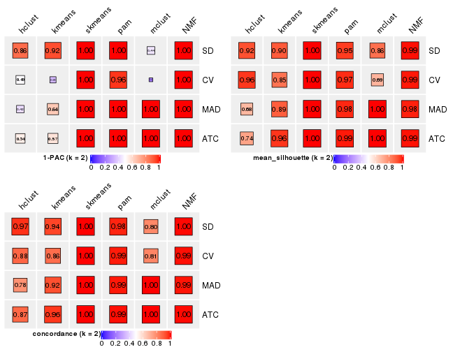
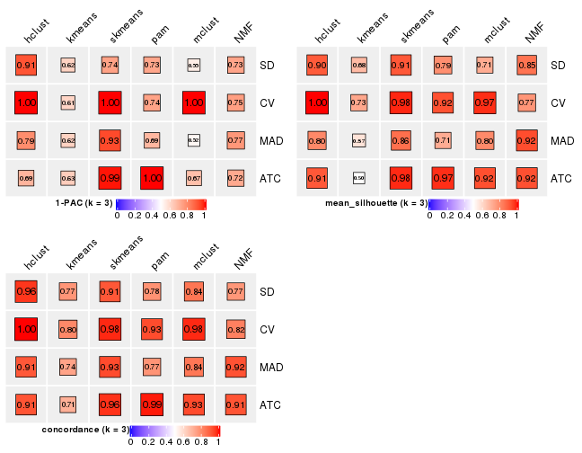
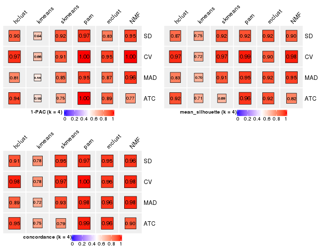
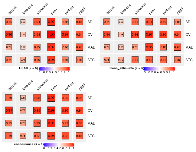
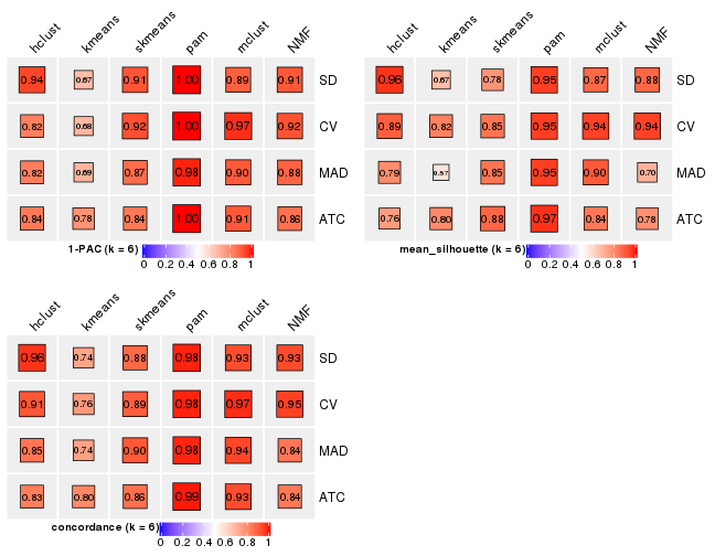
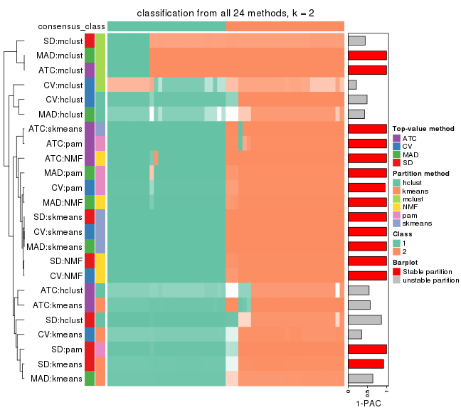
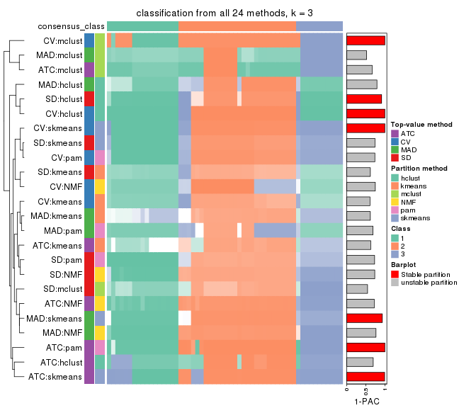
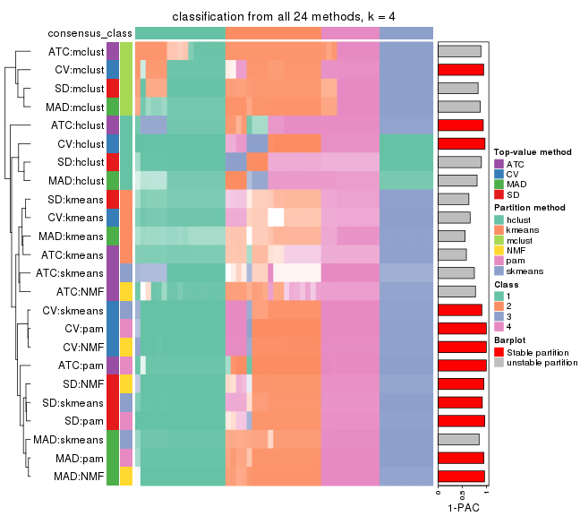
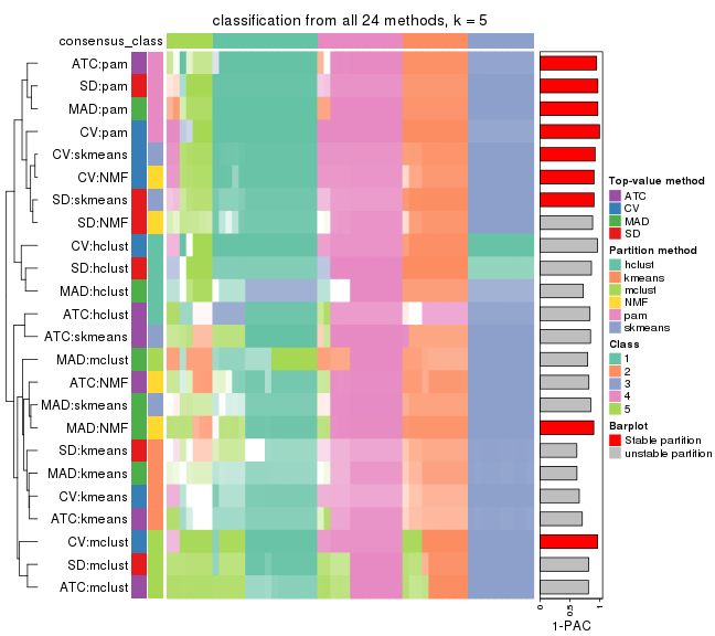
Following heatmap plots the partition for each combination of methods and the lightness correspond to the silhouette scores for samples in each method. On top the consensus subgroup is inferred from all methods by taking the mean silhouette scores as weight.
collect_stats(res_list, k = 2)
collect_stats(res_list, k = 3)
collect_stats(res_list, k = 4)
collect_stats(res_list, k = 5)
collect_stats(res_list, k = 6)
Collect partitions from all methods:
collect_classes(res_list, k = 2)
collect_classes(res_list, k = 3)
collect_classes(res_list, k = 4)
collect_classes(res_list, k = 5)
collect_classes(res_list, k = 6)
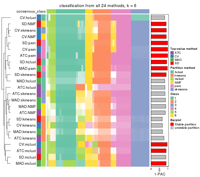
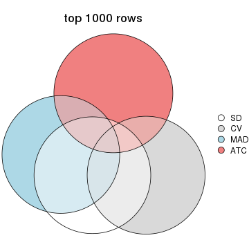
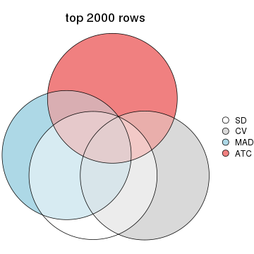
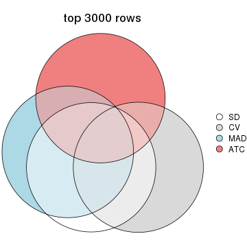
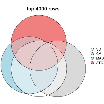
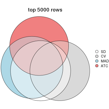
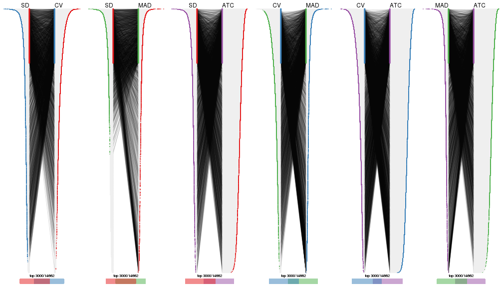
Overlap of top rows from different top-row methods:
top_rows_overlap(res_list, top_n = 1000, method = "euler")
top_rows_overlap(res_list, top_n = 2000, method = "euler")
top_rows_overlap(res_list, top_n = 3000, method = "euler")
top_rows_overlap(res_list, top_n = 4000, method = "euler")
top_rows_overlap(res_list, top_n = 5000, method = "euler")
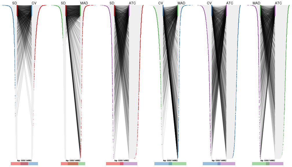
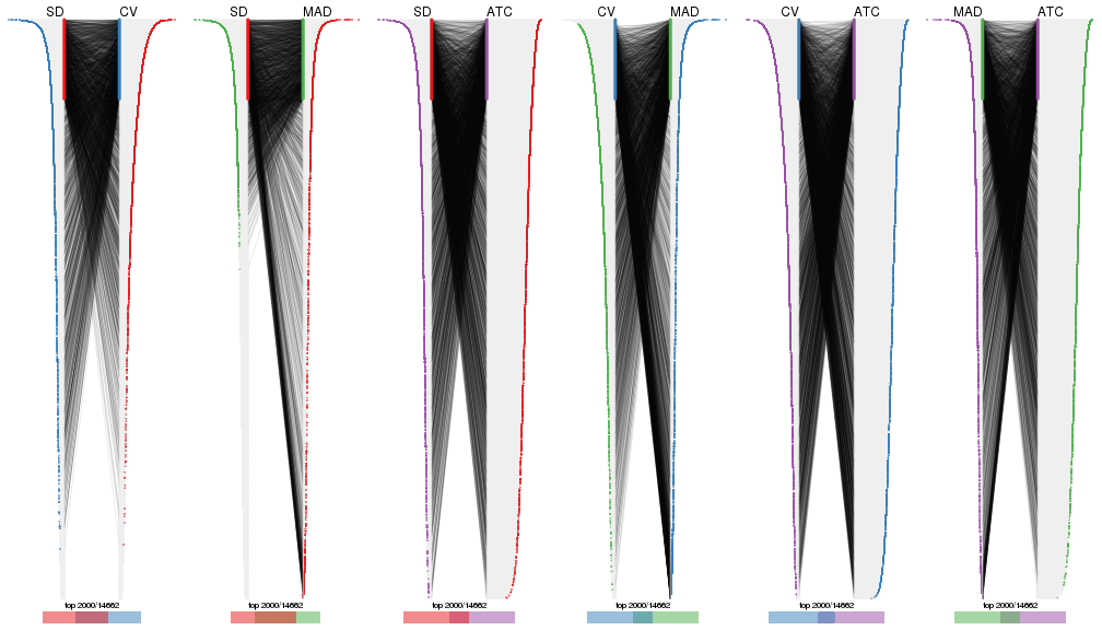
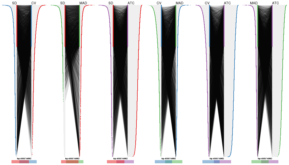
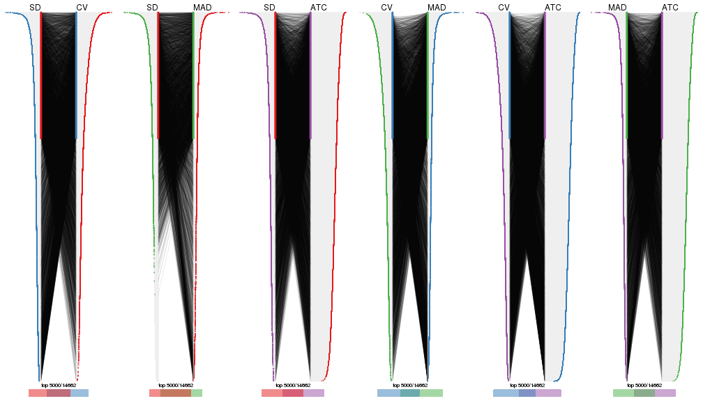
Also visualize the correspondance of rankings between different top-row methods:
top_rows_overlap(res_list, top_n = 1000, method = "correspondance")
top_rows_overlap(res_list, top_n = 2000, method = "correspondance")
top_rows_overlap(res_list, top_n = 3000, method = "correspondance")
top_rows_overlap(res_list, top_n = 4000, method = "correspondance")
top_rows_overlap(res_list, top_n = 5000, method = "correspondance")
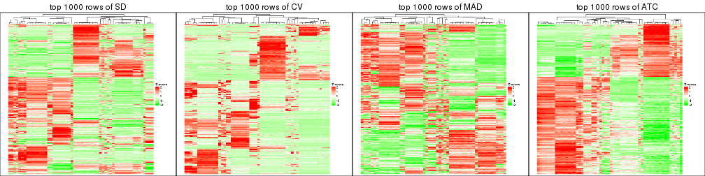
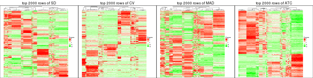
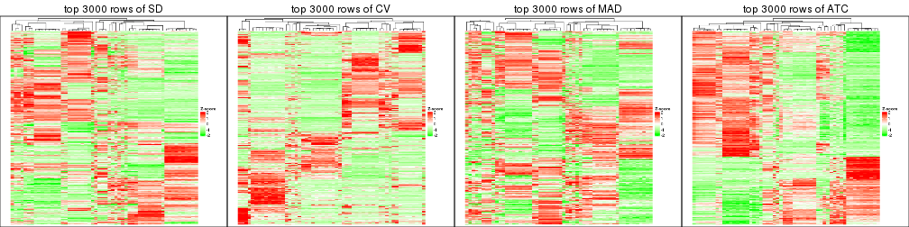
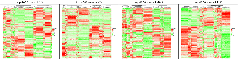
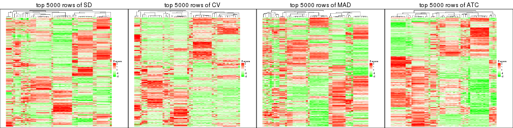
Heatmaps of the top rows:
top_rows_heatmap(res_list, top_n = 1000)
top_rows_heatmap(res_list, top_n = 2000)
top_rows_heatmap(res_list, top_n = 3000)
top_rows_heatmap(res_list, top_n = 4000)
top_rows_heatmap(res_list, top_n = 5000)
The object with results only for a single top-value method and a single partition method can be extracted as:
res = res_list["SD", "hclust"]
# you can also extract it by
# res = res_list["SD:hclust"]
A summary of res and all the functions that can be applied to it:
res
#> A 'ConsensusPartition' object with k = 2, 3, 4, 5, 6.
#>   On a matrix with 14662 rows and 56 columns.
#>   Top rows (1000, 2000, 3000, 4000, 5000) are extracted by 'SD' method.
#>   Subgroups are detected by 'hclust' method.
#>   Performed in total 1250 partitions by row resampling.
#>   Best k for subgroups seems to be 6.
#>
#> Following methods can be applied to this 'ConsensusPartition' object:
#>  [1] "cola_report"             "collect_classes"         "collect_plots"
#>  [4] "collect_stats"           "colnames"                "compare_signatures"
#>  [7] "consensus_heatmap"       "dimension_reduction"     "functional_enrichment"
#> [10] "get_anno_col"            "get_anno"                "get_classes"
#> [13] "get_consensus"           "get_matrix"              "get_membership"
#> [16] "get_param"               "get_signatures"          "get_stats"
#> [19] "is_best_k"               "is_stable_k"             "membership_heatmap"
#> [22] "ncol"                    "nrow"                    "plot_ecdf"
#> [25] "rownames"                "select_partition_number" "show"
#> [28] "suggest_best_k"          "test_to_known_factors"
collect_plots() function collects all the plots made from res for all k (number of partitions)
into one single page to provide an easy and fast comparison between different k.
collect_plots(res)
The plots are:
k and the heatmap of
predicted classes for each k.k.k.k.All the plots in panels can be made by individual functions and they are plotted later in this section.
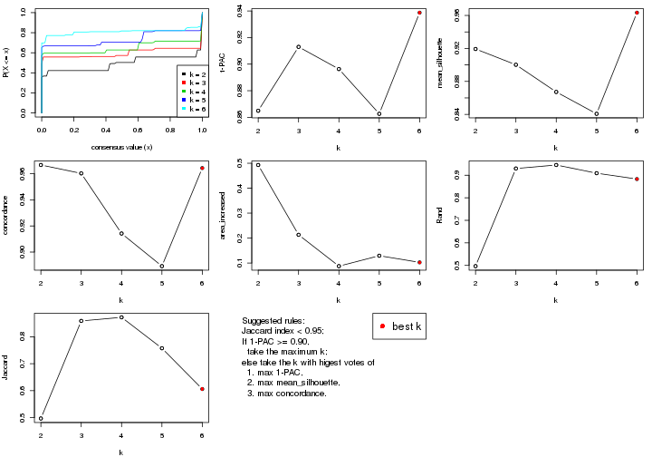
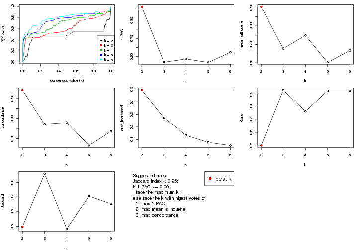
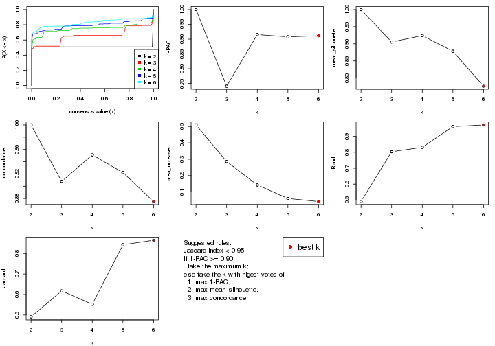
select_partition_number() produces several plots showing different
statistics for choosing “optimized” k. There are following statistics:
k;k, the area increased is defined as \(A_k - A_{k-1}\).The detailed explanations of these statistics can be found in the cola vignette.
Generally speaking, lower PAC score, higher mean silhouette score or higher
concordance corresponds to better partition. Rand index and Jaccard index
measure how similar the current partition is compared to partition with k-1.
If they are too similar, we won't accept k is better than k-1.
select_partition_number(res)
The numeric values for all these statistics can be obtained by get_stats().
get_stats(res)
#>   k 1-PAC mean_silhouette concordance area_increased  Rand Jaccard
#> 2 2 0.865           0.919       0.967         0.4929 0.497   0.497
#> 3 3 0.913           0.900       0.960         0.2131 0.930   0.859
#> 4 4 0.896           0.867       0.914         0.0875 0.945   0.872
#> 5 5 0.863           0.841       0.889         0.1293 0.909   0.757
#> 6 6 0.939           0.963       0.964         0.1026 0.883   0.606
suggest_best_k() suggests the best \(k\) based on these statistics. The rules are as follows:
suggest_best_k(res)
#> [1] 6
#> attr(,"optional")
#> [1] 3
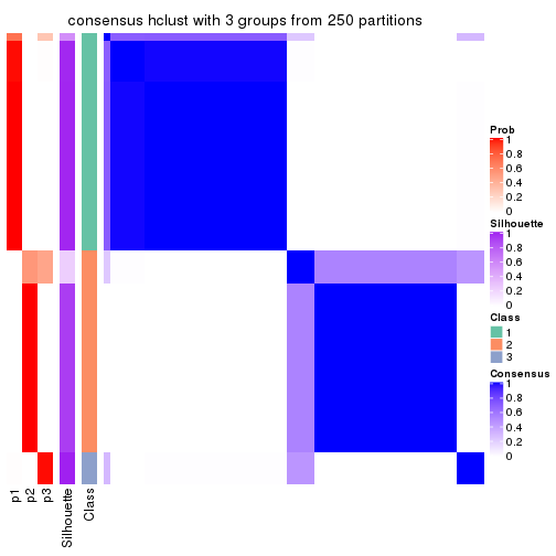
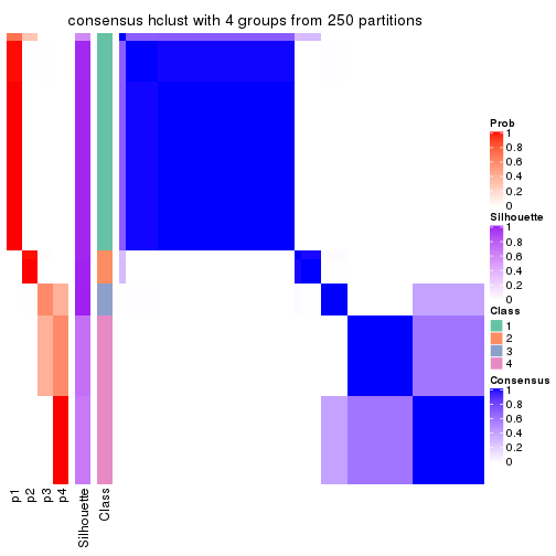
There is also optional best \(k\) = 3 that is worth to check.
Following shows the table of the partitions (You need to click the show/hide
code output link to see it). The membership matrix (columns with name p*)
is inferred by
clue::cl_consensus()
function with the SE method. Basically the value in the membership matrix
represents the probability to belong to a certain group. The finall class
label for an item is determined with the group with highest probability it
belongs to.
In get_classes() function, the entropy is calculated from the membership
matrix and the silhouette score is calculated from the consensus matrix.
cbind(get_classes(res, k = 2), get_membership(res, k = 2))
#>           class entropy silhouette    p1    p2
#> SRR073723     1  0.0672      0.987 0.992 0.008
#> SRR073724     1  0.0000      0.994 1.000 0.000
#> SRR073725     1  0.0000      0.994 1.000 0.000
#> SRR073726     2  0.9833      0.344 0.424 0.576
#> SRR073727     1  0.0000      0.994 1.000 0.000
#> SRR073728     1  0.2423      0.959 0.960 0.040
#> SRR073729     1  0.2423      0.959 0.960 0.040
#> SRR073730     1  0.2423      0.959 0.960 0.040
#> SRR073731     2  0.0000      0.926 0.000 1.000
#> SRR073732     2  0.0000      0.926 0.000 1.000
#> SRR073733     2  0.0000      0.926 0.000 1.000
#> SRR073734     2  0.0000      0.926 0.000 1.000
#> SRR073735     2  0.0000      0.926 0.000 1.000
#> SRR073736     2  0.0000      0.926 0.000 1.000
#> SRR073737     2  0.0000      0.926 0.000 1.000
#> SRR073738     1  0.0000      0.994 1.000 0.000
#> SRR073739     1  0.0000      0.994 1.000 0.000
#> SRR073740     1  0.0000      0.994 1.000 0.000
#> SRR073741     1  0.0000      0.994 1.000 0.000
#> SRR073742     1  0.0000      0.994 1.000 0.000
#> SRR073743     1  0.0000      0.994 1.000 0.000
#> SRR073744     1  0.0000      0.994 1.000 0.000
#> SRR073745     1  0.0000      0.994 1.000 0.000
#> SRR073746     1  0.0000      0.994 1.000 0.000
#> SRR073747     1  0.0000      0.994 1.000 0.000
#> SRR073748     1  0.0000      0.994 1.000 0.000
#> SRR073749     1  0.0000      0.994 1.000 0.000
#> SRR073750     1  0.0000      0.994 1.000 0.000
#> SRR073751     1  0.2423      0.959 0.960 0.040
#> SRR073752     2  0.0000      0.926 0.000 1.000
#> SRR073753     2  0.0000      0.926 0.000 1.000
#> SRR073754     2  0.9833      0.344 0.424 0.576
#> SRR073755     2  0.0000      0.926 0.000 1.000
#> SRR073756     2  0.0000      0.926 0.000 1.000
#> SRR073758     2  0.0000      0.926 0.000 1.000
#> SRR073759     2  0.0000      0.926 0.000 1.000
#> SRR073760     2  0.0000      0.926 0.000 1.000
#> SRR073761     2  0.0000      0.926 0.000 1.000
#> SRR073763     2  0.0000      0.926 0.000 1.000
#> SRR073764     2  0.0000      0.926 0.000 1.000
#> SRR073765     2  0.0000      0.926 0.000 1.000
#> SRR073766     2  0.0000      0.926 0.000 1.000
#> SRR073767     2  0.0000      0.926 0.000 1.000
#> SRR073768     2  0.0000      0.926 0.000 1.000
#> SRR073769     1  0.0000      0.994 1.000 0.000
#> SRR073770     1  0.0000      0.994 1.000 0.000
#> SRR073771     1  0.0000      0.994 1.000 0.000
#> SRR073772     1  0.0000      0.994 1.000 0.000
#> SRR073773     1  0.0000      0.994 1.000 0.000
#> SRR073774     1  0.0000      0.994 1.000 0.000
#> SRR073775     1  0.0000      0.994 1.000 0.000
#> SRR073776     1  0.0000      0.994 1.000 0.000
#> SRR073777     1  0.0000      0.994 1.000 0.000
#> SRR073778     1  0.0000      0.994 1.000 0.000
#> SRR073779     2  0.9833      0.344 0.424 0.576
#> SRR073780     2  0.9833      0.344 0.424 0.576
cbind(get_classes(res, k = 3), get_membership(res, k = 3))
#>           class entropy silhouette    p1    p2    p3
#> SRR073723     1  0.5529      0.561 0.704 0.000 0.296
#> SRR073724     1  0.0424      0.981 0.992 0.000 0.008
#> SRR073725     1  0.0424      0.981 0.992 0.000 0.008
#> SRR073726     2  0.6286      0.244 0.000 0.536 0.464
#> SRR073727     1  0.0424      0.981 0.992 0.000 0.008
#> SRR073728     3  0.0424      1.000 0.008 0.000 0.992
#> SRR073729     3  0.0424      1.000 0.008 0.000 0.992
#> SRR073730     3  0.0424      1.000 0.008 0.000 0.992
#> SRR073731     2  0.0000      0.917 0.000 1.000 0.000
#> SRR073732     2  0.0000      0.917 0.000 1.000 0.000
#> SRR073733     2  0.0000      0.917 0.000 1.000 0.000
#> SRR073734     2  0.0000      0.917 0.000 1.000 0.000
#> SRR073735     2  0.0000      0.917 0.000 1.000 0.000
#> SRR073736     2  0.0000      0.917 0.000 1.000 0.000
#> SRR073737     2  0.0000      0.917 0.000 1.000 0.000
#> SRR073738     1  0.0424      0.981 0.992 0.000 0.008
#> SRR073739     1  0.0000      0.986 1.000 0.000 0.000
#> SRR073740     1  0.0000      0.986 1.000 0.000 0.000
#> SRR073741     1  0.0000      0.986 1.000 0.000 0.000
#> SRR073742     1  0.0000      0.986 1.000 0.000 0.000
#> SRR073743     1  0.0000      0.986 1.000 0.000 0.000
#> SRR073744     1  0.0000      0.986 1.000 0.000 0.000
#> SRR073745     1  0.0000      0.986 1.000 0.000 0.000
#> SRR073746     1  0.0000      0.986 1.000 0.000 0.000
#> SRR073747     1  0.0000      0.986 1.000 0.000 0.000
#> SRR073748     1  0.0000      0.986 1.000 0.000 0.000
#> SRR073749     1  0.0000      0.986 1.000 0.000 0.000
#> SRR073750     1  0.0424      0.981 0.992 0.000 0.008
#> SRR073751     3  0.0424      1.000 0.008 0.000 0.992
#> SRR073752     2  0.0000      0.917 0.000 1.000 0.000
#> SRR073753     2  0.0000      0.917 0.000 1.000 0.000
#> SRR073754     2  0.6286      0.244 0.000 0.536 0.464
#> SRR073755     2  0.0000      0.917 0.000 1.000 0.000
#> SRR073756     2  0.0000      0.917 0.000 1.000 0.000
#> SRR073758     2  0.0000      0.917 0.000 1.000 0.000
#> SRR073759     2  0.0000      0.917 0.000 1.000 0.000
#> SRR073760     2  0.0000      0.917 0.000 1.000 0.000
#> SRR073761     2  0.0000      0.917 0.000 1.000 0.000
#> SRR073763     2  0.0000      0.917 0.000 1.000 0.000
#> SRR073764     2  0.0000      0.917 0.000 1.000 0.000
#> SRR073765     2  0.0000      0.917 0.000 1.000 0.000
#> SRR073766     2  0.0000      0.917 0.000 1.000 0.000
#> SRR073767     2  0.0000      0.917 0.000 1.000 0.000
#> SRR073768     2  0.0000      0.917 0.000 1.000 0.000
#> SRR073769     1  0.0000      0.986 1.000 0.000 0.000
#> SRR073770     1  0.0000      0.986 1.000 0.000 0.000
#> SRR073771     1  0.0000      0.986 1.000 0.000 0.000
#> SRR073772     1  0.0000      0.986 1.000 0.000 0.000
#> SRR073773     1  0.0000      0.986 1.000 0.000 0.000
#> SRR073774     1  0.0000      0.986 1.000 0.000 0.000
#> SRR073775     1  0.0000      0.986 1.000 0.000 0.000
#> SRR073776     1  0.0000      0.986 1.000 0.000 0.000
#> SRR073777     1  0.0000      0.986 1.000 0.000 0.000
#> SRR073778     1  0.0000      0.986 1.000 0.000 0.000
#> SRR073779     2  0.6286      0.244 0.000 0.536 0.464
#> SRR073780     2  0.6286      0.244 0.000 0.536 0.464
cbind(get_classes(res, k = 4), get_membership(res, k = 4))
#>           class entropy silhouette    p1    p2    p3    p4
#> SRR073723     1  0.4382      0.580 0.704 0.296 0.000 0.000
#> SRR073724     1  0.0336      0.982 0.992 0.000 0.008 0.000
#> SRR073725     1  0.0336      0.982 0.992 0.000 0.008 0.000
#> SRR073726     3  0.5028      1.000 0.000 0.004 0.596 0.400
#> SRR073727     1  0.0336      0.982 0.992 0.000 0.008 0.000
#> SRR073728     2  0.0000      0.996 0.000 1.000 0.000 0.000
#> SRR073729     2  0.0000      0.996 0.000 1.000 0.000 0.000
#> SRR073730     2  0.0000      0.996 0.000 1.000 0.000 0.000
#> SRR073731     4  0.4866      0.708 0.000 0.000 0.404 0.596
#> SRR073732     4  0.4866      0.708 0.000 0.000 0.404 0.596
#> SRR073733     4  0.4866      0.708 0.000 0.000 0.404 0.596
#> SRR073734     4  0.4866      0.708 0.000 0.000 0.404 0.596
#> SRR073735     4  0.4866      0.708 0.000 0.000 0.404 0.596
#> SRR073736     4  0.4866      0.708 0.000 0.000 0.404 0.596
#> SRR073737     4  0.4866      0.708 0.000 0.000 0.404 0.596
#> SRR073738     1  0.0336      0.982 0.992 0.000 0.008 0.000
#> SRR073739     1  0.0000      0.987 1.000 0.000 0.000 0.000
#> SRR073740     1  0.0000      0.987 1.000 0.000 0.000 0.000
#> SRR073741     1  0.0000      0.987 1.000 0.000 0.000 0.000
#> SRR073742     1  0.0000      0.987 1.000 0.000 0.000 0.000
#> SRR073743     1  0.0000      0.987 1.000 0.000 0.000 0.000
#> SRR073744     1  0.0000      0.987 1.000 0.000 0.000 0.000
#> SRR073745     1  0.0000      0.987 1.000 0.000 0.000 0.000
#> SRR073746     1  0.0000      0.987 1.000 0.000 0.000 0.000
#> SRR073747     1  0.0000      0.987 1.000 0.000 0.000 0.000
#> SRR073748     1  0.0000      0.987 1.000 0.000 0.000 0.000
#> SRR073749     1  0.0000      0.987 1.000 0.000 0.000 0.000
#> SRR073750     1  0.0336      0.982 0.992 0.000 0.008 0.000
#> SRR073751     2  0.0469      0.988 0.000 0.988 0.012 0.000
#> SRR073752     4  0.4866      0.708 0.000 0.000 0.404 0.596
#> SRR073753     4  0.4866      0.708 0.000 0.000 0.404 0.596
#> SRR073754     3  0.5028      1.000 0.000 0.004 0.596 0.400
#> SRR073755     4  0.0000      0.663 0.000 0.000 0.000 1.000
#> SRR073756     4  0.0000      0.663 0.000 0.000 0.000 1.000
#> SRR073758     4  0.0000      0.663 0.000 0.000 0.000 1.000
#> SRR073759     4  0.4866      0.708 0.000 0.000 0.404 0.596
#> SRR073760     4  0.0000      0.663 0.000 0.000 0.000 1.000
#> SRR073761     4  0.0000      0.663 0.000 0.000 0.000 1.000
#> SRR073763     4  0.0000      0.663 0.000 0.000 0.000 1.000
#> SRR073764     4  0.0000      0.663 0.000 0.000 0.000 1.000
#> SRR073765     4  0.0000      0.663 0.000 0.000 0.000 1.000
#> SRR073766     4  0.0000      0.663 0.000 0.000 0.000 1.000
#> SRR073767     4  0.0000      0.663 0.000 0.000 0.000 1.000
#> SRR073768     4  0.0000      0.663 0.000 0.000 0.000 1.000
#> SRR073769     1  0.0000      0.987 1.000 0.000 0.000 0.000
#> SRR073770     1  0.0000      0.987 1.000 0.000 0.000 0.000
#> SRR073771     1  0.0000      0.987 1.000 0.000 0.000 0.000
#> SRR073772     1  0.0000      0.987 1.000 0.000 0.000 0.000
#> SRR073773     1  0.0000      0.987 1.000 0.000 0.000 0.000
#> SRR073774     1  0.0000      0.987 1.000 0.000 0.000 0.000
#> SRR073775     1  0.0000      0.987 1.000 0.000 0.000 0.000
#> SRR073776     1  0.0000      0.987 1.000 0.000 0.000 0.000
#> SRR073777     1  0.0000      0.987 1.000 0.000 0.000 0.000
#> SRR073778     1  0.0000      0.987 1.000 0.000 0.000 0.000
#> SRR073779     3  0.5028      1.000 0.000 0.004 0.596 0.400
#> SRR073780     3  0.5028      1.000 0.000 0.004 0.596 0.400
cbind(get_classes(res, k = 5), get_membership(res, k = 5))
#>           class entropy silhouette    p1 p2    p3    p4    p5
#> SRR073723     3  0.6802     -0.524 0.336  0 0.368 0.000 0.296
#> SRR073724     1  0.4114      0.820 0.624  0 0.376 0.000 0.000
#> SRR073725     1  0.4114      0.820 0.624  0 0.376 0.000 0.000
#> SRR073726     3  0.4088      0.594 0.000  0 0.632 0.368 0.000
#> SRR073727     1  0.4114      0.820 0.624  0 0.376 0.000 0.000
#> SRR073728     5  0.0000      0.996 0.000  0 0.000 0.000 1.000
#> SRR073729     5  0.0000      0.996 0.000  0 0.000 0.000 1.000
#> SRR073730     5  0.0000      0.996 0.000  0 0.000 0.000 1.000
#> SRR073731     2  0.0000      1.000 0.000  1 0.000 0.000 0.000
#> SRR073732     2  0.0000      1.000 0.000  1 0.000 0.000 0.000
#> SRR073733     2  0.0000      1.000 0.000  1 0.000 0.000 0.000
#> SRR073734     2  0.0000      1.000 0.000  1 0.000 0.000 0.000
#> SRR073735     2  0.0000      1.000 0.000  1 0.000 0.000 0.000
#> SRR073736     2  0.0000      1.000 0.000  1 0.000 0.000 0.000
#> SRR073737     2  0.0000      1.000 0.000  1 0.000 0.000 0.000
#> SRR073738     1  0.4114      0.820 0.624  0 0.376 0.000 0.000
#> SRR073739     1  0.4088      0.824 0.632  0 0.368 0.000 0.000
#> SRR073740     1  0.4088      0.824 0.632  0 0.368 0.000 0.000
#> SRR073741     1  0.4088      0.824 0.632  0 0.368 0.000 0.000
#> SRR073742     1  0.4088      0.824 0.632  0 0.368 0.000 0.000
#> SRR073743     1  0.4088      0.824 0.632  0 0.368 0.000 0.000
#> SRR073744     1  0.4088      0.824 0.632  0 0.368 0.000 0.000
#> SRR073745     1  0.4088      0.824 0.632  0 0.368 0.000 0.000
#> SRR073746     1  0.4088      0.824 0.632  0 0.368 0.000 0.000
#> SRR073747     1  0.4088      0.824 0.632  0 0.368 0.000 0.000
#> SRR073748     1  0.4088      0.824 0.632  0 0.368 0.000 0.000
#> SRR073749     1  0.4088      0.824 0.632  0 0.368 0.000 0.000
#> SRR073750     1  0.4114      0.820 0.624  0 0.376 0.000 0.000
#> SRR073751     5  0.0404      0.988 0.000  0 0.012 0.000 0.988
#> SRR073752     2  0.0000      1.000 0.000  1 0.000 0.000 0.000
#> SRR073753     2  0.0000      1.000 0.000  1 0.000 0.000 0.000
#> SRR073754     3  0.4088      0.594 0.000  0 0.632 0.368 0.000
#> SRR073755     4  0.0000      1.000 0.000  0 0.000 1.000 0.000
#> SRR073756     4  0.0000      1.000 0.000  0 0.000 1.000 0.000
#> SRR073758     4  0.0000      1.000 0.000  0 0.000 1.000 0.000
#> SRR073759     2  0.0000      1.000 0.000  1 0.000 0.000 0.000
#> SRR073760     4  0.0000      1.000 0.000  0 0.000 1.000 0.000
#> SRR073761     4  0.0000      1.000 0.000  0 0.000 1.000 0.000
#> SRR073763     4  0.0000      1.000 0.000  0 0.000 1.000 0.000
#> SRR073764     4  0.0000      1.000 0.000  0 0.000 1.000 0.000
#> SRR073765     4  0.0000      1.000 0.000  0 0.000 1.000 0.000
#> SRR073766     4  0.0000      1.000 0.000  0 0.000 1.000 0.000
#> SRR073767     4  0.0000      1.000 0.000  0 0.000 1.000 0.000
#> SRR073768     4  0.0000      1.000 0.000  0 0.000 1.000 0.000
#> SRR073769     1  0.0000      0.709 1.000  0 0.000 0.000 0.000
#> SRR073770     1  0.0000      0.709 1.000  0 0.000 0.000 0.000
#> SRR073771     1  0.0000      0.709 1.000  0 0.000 0.000 0.000
#> SRR073772     1  0.0000      0.709 1.000  0 0.000 0.000 0.000
#> SRR073773     1  0.0000      0.709 1.000  0 0.000 0.000 0.000
#> SRR073774     1  0.0000      0.709 1.000  0 0.000 0.000 0.000
#> SRR073775     1  0.0000      0.709 1.000  0 0.000 0.000 0.000
#> SRR073776     1  0.0000      0.709 1.000  0 0.000 0.000 0.000
#> SRR073777     1  0.0000      0.709 1.000  0 0.000 0.000 0.000
#> SRR073778     1  0.0000      0.709 1.000  0 0.000 0.000 0.000
#> SRR073779     3  0.4088      0.594 0.000  0 0.632 0.368 0.000
#> SRR073780     3  0.4088      0.594 0.000  0 0.632 0.368 0.000
cbind(get_classes(res, k = 6), get_membership(res, k = 6))
#>           class entropy silhouette    p1 p2    p3    p4    p5    p6
#> SRR073723     1  0.6689      0.211 0.476  0 0.148 0.000 0.296 0.080
#> SRR073724     1  0.1556      0.898 0.920  0 0.000 0.000 0.000 0.080
#> SRR073725     1  0.0000      0.932 1.000  0 0.000 0.000 0.000 0.000
#> SRR073726     6  0.2730      1.000 0.000  0 0.000 0.192 0.000 0.808
#> SRR073727     1  0.1556      0.898 0.920  0 0.000 0.000 0.000 0.080
#> SRR073728     5  0.0000      0.971 0.000  0 0.000 0.000 1.000 0.000
#> SRR073729     5  0.0000      0.971 0.000  0 0.000 0.000 1.000 0.000
#> SRR073730     5  0.0000      0.971 0.000  0 0.000 0.000 1.000 0.000
#> SRR073731     2  0.0000      1.000 0.000  1 0.000 0.000 0.000 0.000
#> SRR073732     2  0.0000      1.000 0.000  1 0.000 0.000 0.000 0.000
#> SRR073733     2  0.0000      1.000 0.000  1 0.000 0.000 0.000 0.000
#> SRR073734     2  0.0000      1.000 0.000  1 0.000 0.000 0.000 0.000
#> SRR073735     2  0.0000      1.000 0.000  1 0.000 0.000 0.000 0.000
#> SRR073736     2  0.0000      1.000 0.000  1 0.000 0.000 0.000 0.000
#> SRR073737     2  0.0000      1.000 0.000  1 0.000 0.000 0.000 0.000
#> SRR073738     1  0.1556      0.898 0.920  0 0.000 0.000 0.000 0.080
#> SRR073739     1  0.0632      0.945 0.976  0 0.024 0.000 0.000 0.000
#> SRR073740     1  0.0632      0.945 0.976  0 0.024 0.000 0.000 0.000
#> SRR073741     1  0.0632      0.945 0.976  0 0.024 0.000 0.000 0.000
#> SRR073742     1  0.0632      0.945 0.976  0 0.024 0.000 0.000 0.000
#> SRR073743     1  0.0632      0.945 0.976  0 0.024 0.000 0.000 0.000
#> SRR073744     1  0.0632      0.945 0.976  0 0.024 0.000 0.000 0.000
#> SRR073745     1  0.0632      0.945 0.976  0 0.024 0.000 0.000 0.000
#> SRR073746     1  0.0632      0.945 0.976  0 0.024 0.000 0.000 0.000
#> SRR073747     1  0.0632      0.945 0.976  0 0.024 0.000 0.000 0.000
#> SRR073748     1  0.0632      0.945 0.976  0 0.024 0.000 0.000 0.000
#> SRR073749     1  0.0632      0.945 0.976  0 0.024 0.000 0.000 0.000
#> SRR073750     1  0.1501      0.900 0.924  0 0.000 0.000 0.000 0.076
#> SRR073751     5  0.2092      0.910 0.000  0 0.000 0.000 0.876 0.124
#> SRR073752     2  0.0000      1.000 0.000  1 0.000 0.000 0.000 0.000
#> SRR073753     2  0.0000      1.000 0.000  1 0.000 0.000 0.000 0.000
#> SRR073754     6  0.2730      1.000 0.000  0 0.000 0.192 0.000 0.808
#> SRR073755     4  0.0000      1.000 0.000  0 0.000 1.000 0.000 0.000
#> SRR073756     4  0.0000      1.000 0.000  0 0.000 1.000 0.000 0.000
#> SRR073758     4  0.0000      1.000 0.000  0 0.000 1.000 0.000 0.000
#> SRR073759     2  0.0000      1.000 0.000  1 0.000 0.000 0.000 0.000
#> SRR073760     4  0.0000      1.000 0.000  0 0.000 1.000 0.000 0.000
#> SRR073761     4  0.0000      1.000 0.000  0 0.000 1.000 0.000 0.000
#> SRR073763     4  0.0000      1.000 0.000  0 0.000 1.000 0.000 0.000
#> SRR073764     4  0.0000      1.000 0.000  0 0.000 1.000 0.000 0.000
#> SRR073765     4  0.0000      1.000 0.000  0 0.000 1.000 0.000 0.000
#> SRR073766     4  0.0000      1.000 0.000  0 0.000 1.000 0.000 0.000
#> SRR073767     4  0.0000      1.000 0.000  0 0.000 1.000 0.000 0.000
#> SRR073768     4  0.0000      1.000 0.000  0 0.000 1.000 0.000 0.000
#> SRR073769     3  0.0000      1.000 0.000  0 1.000 0.000 0.000 0.000
#> SRR073770     3  0.0000      1.000 0.000  0 1.000 0.000 0.000 0.000
#> SRR073771     3  0.0000      1.000 0.000  0 1.000 0.000 0.000 0.000
#> SRR073772     3  0.0000      1.000 0.000  0 1.000 0.000 0.000 0.000
#> SRR073773     3  0.0000      1.000 0.000  0 1.000 0.000 0.000 0.000
#> SRR073774     3  0.0000      1.000 0.000  0 1.000 0.000 0.000 0.000
#> SRR073775     3  0.0000      1.000 0.000  0 1.000 0.000 0.000 0.000
#> SRR073776     3  0.0000      1.000 0.000  0 1.000 0.000 0.000 0.000
#> SRR073777     3  0.0000      1.000 0.000  0 1.000 0.000 0.000 0.000
#> SRR073778     3  0.0000      1.000 0.000  0 1.000 0.000 0.000 0.000
#> SRR073779     6  0.2730      1.000 0.000  0 0.000 0.192 0.000 0.808
#> SRR073780     6  0.2730      1.000 0.000  0 0.000 0.192 0.000 0.808
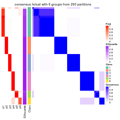
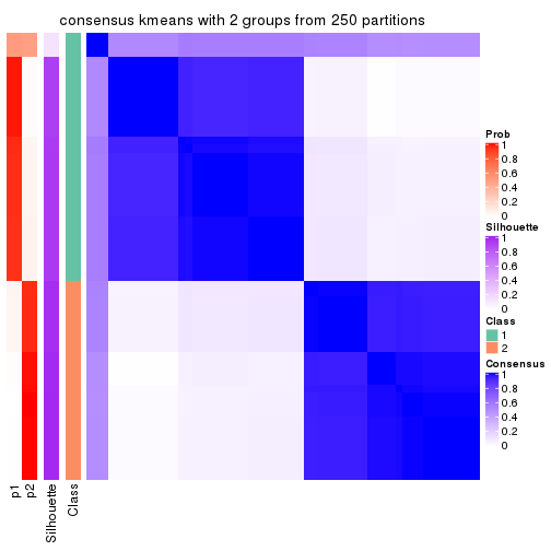
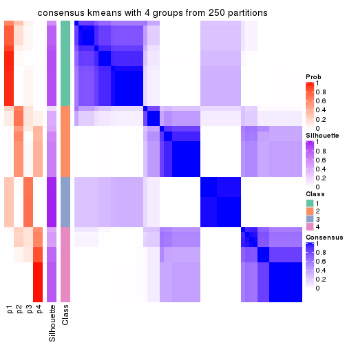
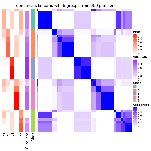
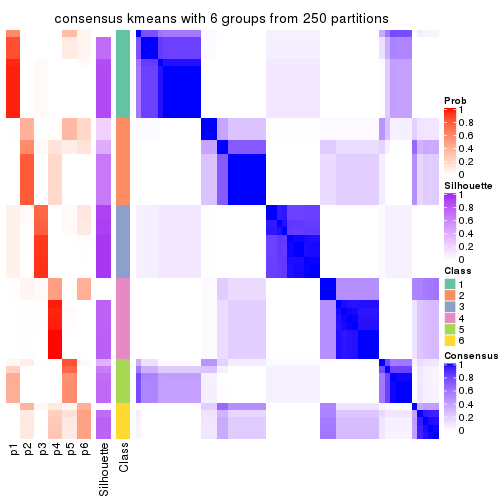
Heatmaps for the consensus matrix. It visualizes the probability of two samples to be in a same group.
consensus_heatmap(res, k = 2)

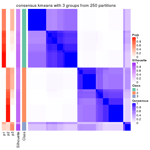
consensus_heatmap(res, k = 3)
consensus_heatmap(res, k = 4)
consensus_heatmap(res, k = 5)
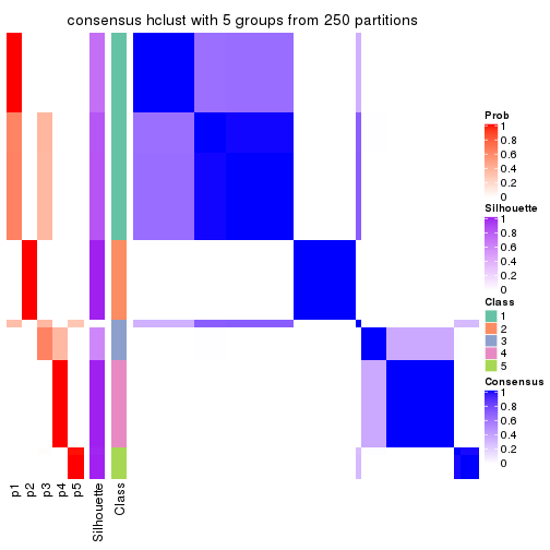
consensus_heatmap(res, k = 6)
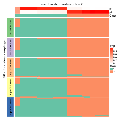
Heatmaps for the membership of samples in all partitions to see how consistent they are:
membership_heatmap(res, k = 2)
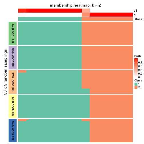
membership_heatmap(res, k = 3)
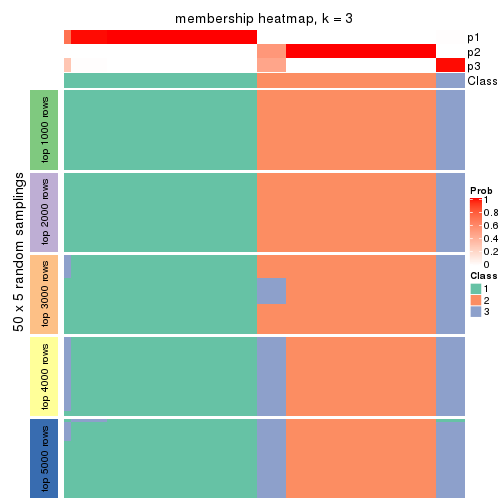
membership_heatmap(res, k = 4)
membership_heatmap(res, k = 5)
membership_heatmap(res, k = 6)
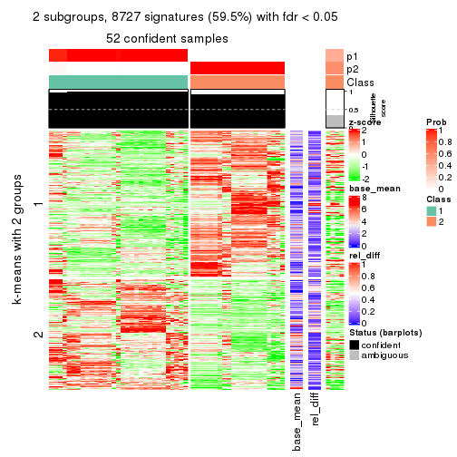
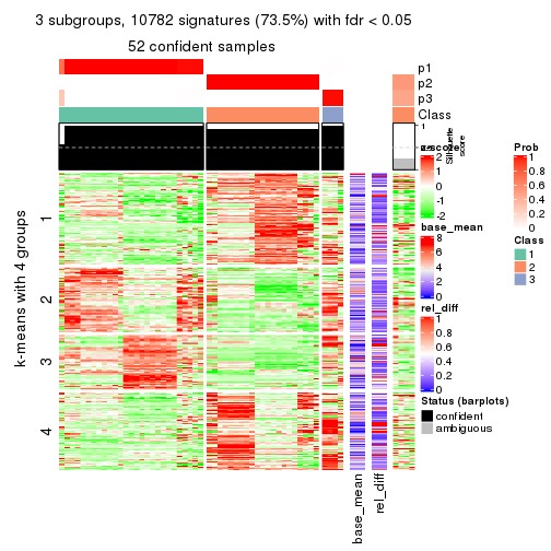
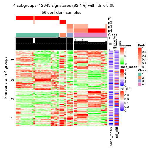
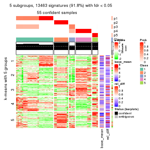
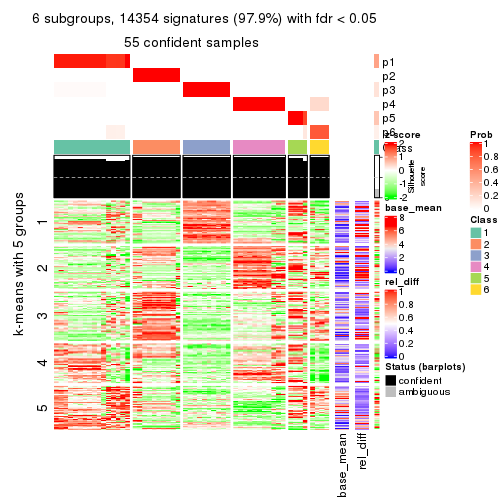
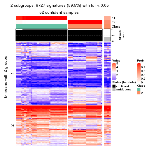
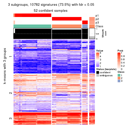
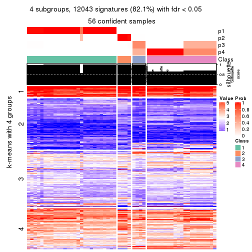
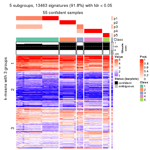
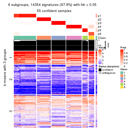
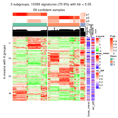
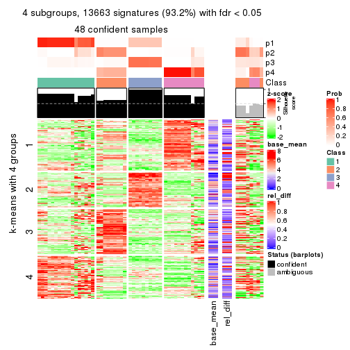
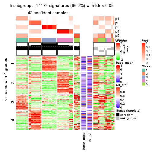
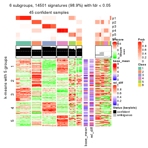
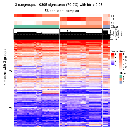
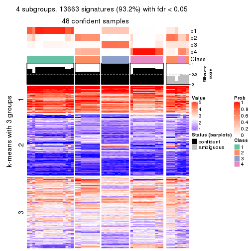
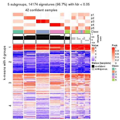
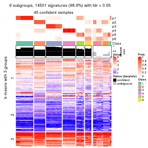
As soon as we have had the classes for columns, we can look for signatures which are significantly different between classes which can be candidate marks for certain classes. Following are the heatmaps for signatures.
Signature heatmaps where rows are scaled:
get_signatures(res, k = 2)
get_signatures(res, k = 3)
get_signatures(res, k = 4)
get_signatures(res, k = 5)
get_signatures(res, k = 6)
Signature heatmaps where rows are not scaled:
get_signatures(res, k = 2, scale_rows = FALSE)
get_signatures(res, k = 3, scale_rows = FALSE)
get_signatures(res, k = 4, scale_rows = FALSE)
get_signatures(res, k = 5, scale_rows = FALSE)
get_signatures(res, k = 6, scale_rows = FALSE)
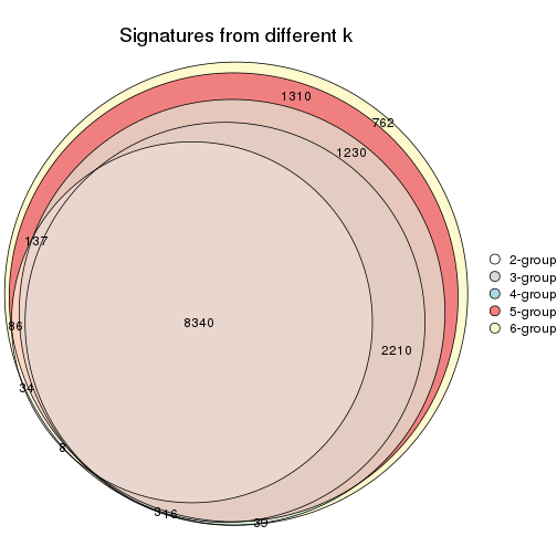
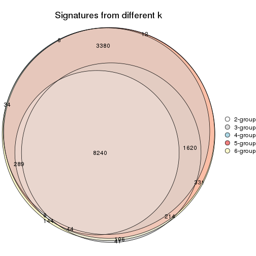
Compare the overlap of signatures from different k:
compare_signatures(res)
get_signature() returns a data frame invisibly. TO get the list of signatures, the function
call should be assigned to a variable explicitly. In following code, if plot argument is set
to FALSE, no heatmap is plotted while only the differential analysis is performed.
# code only for demonstration
tb = get_signature(res, k = ..., plot = FALSE)
An example of the output of tb is:
#>   which_row         fdr    mean_1    mean_2 scaled_mean_1 scaled_mean_2 km
#> 1        38 0.042760348  8.373488  9.131774    -0.5533452     0.5164555  1
#> 2        40 0.018707592  7.106213  8.469186    -0.6173731     0.5762149  1
#> 3        55 0.019134737 10.221463 11.207825    -0.6159697     0.5749050  1
#> 4        59 0.006059896  5.921854  7.869574    -0.6899429     0.6439467  1
#> 5        60 0.018055526  8.928898 10.211722    -0.6204761     0.5791110  1
#> 6        98 0.009384629 15.714769 14.887706     0.6635654    -0.6193277  2
...
The columns in tb are:
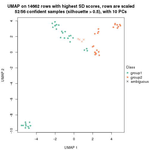
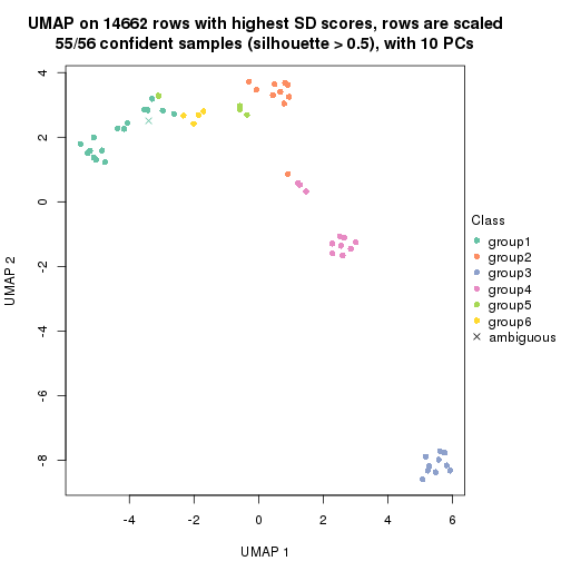
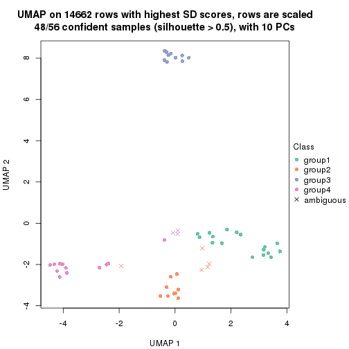
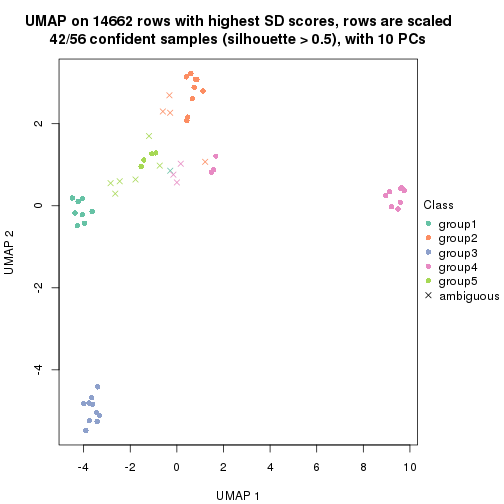
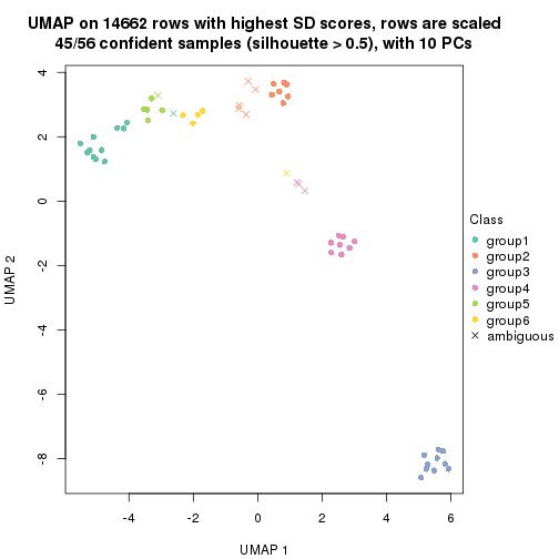
which_row: row indices corresponding to the input matrix.fdr: FDR for the differential test. mean_x: The mean value in group x.scaled_mean_x: The mean value in group x after rows are scaled.km: Row groups if k-means clustering is applied to rows.UMAP plot which shows how samples are separated.
dimension_reduction(res, k = 2, method = "UMAP")
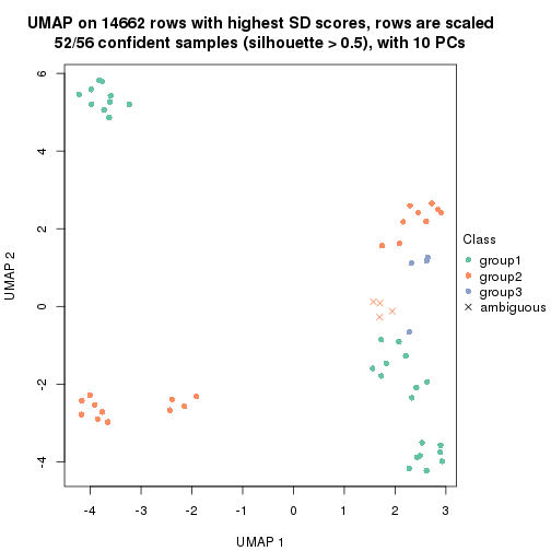
dimension_reduction(res, k = 3, method = "UMAP")
dimension_reduction(res, k = 4, method = "UMAP")
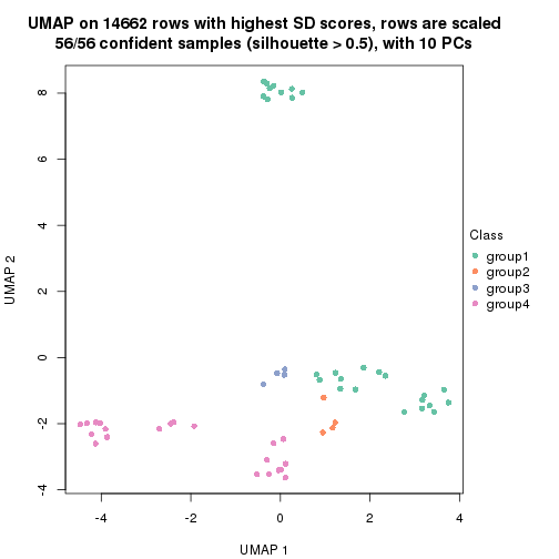
dimension_reduction(res, k = 5, method = "UMAP")
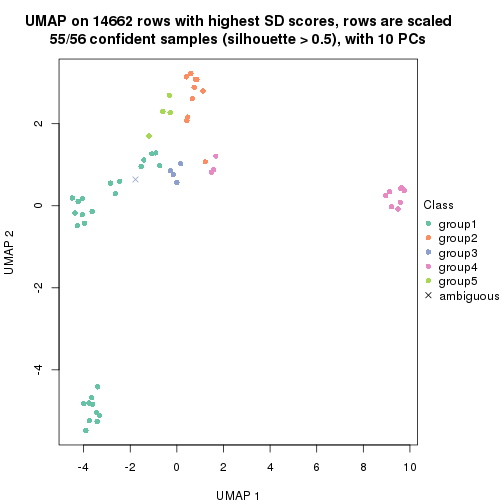
dimension_reduction(res, k = 6, method = "UMAP")
Following heatmap shows how subgroups are split when increasing k:
collect_classes(res)
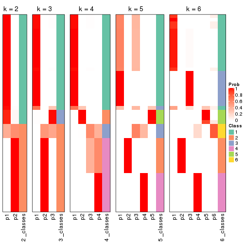
If matrix rows can be associated to genes, consider to use functional_enrichment(res,
...) to perform function enrichment for the signature genes. See this vignette for more detailed explanations.
The object with results only for a single top-value method and a single partition method can be extracted as:
res = res_list["SD", "kmeans"]
# you can also extract it by
# res = res_list["SD:kmeans"]
A summary of res and all the functions that can be applied to it:
res
#> A 'ConsensusPartition' object with k = 2, 3, 4, 5, 6.
#>   On a matrix with 14662 rows and 56 columns.
#>   Top rows (1000, 2000, 3000, 4000, 5000) are extracted by 'SD' method.
#>   Subgroups are detected by 'kmeans' method.
#>   Performed in total 1250 partitions by row resampling.
#>   Best k for subgroups seems to be 2.
#>
#> Following methods can be applied to this 'ConsensusPartition' object:
#>  [1] "cola_report"             "collect_classes"         "collect_plots"
#>  [4] "collect_stats"           "colnames"                "compare_signatures"
#>  [7] "consensus_heatmap"       "dimension_reduction"     "functional_enrichment"
#> [10] "get_anno_col"            "get_anno"                "get_classes"
#> [13] "get_consensus"           "get_matrix"              "get_membership"
#> [16] "get_param"               "get_signatures"          "get_stats"
#> [19] "is_best_k"               "is_stable_k"             "membership_heatmap"
#> [22] "ncol"                    "nrow"                    "plot_ecdf"
#> [25] "rownames"                "select_partition_number" "show"
#> [28] "suggest_best_k"          "test_to_known_factors"
collect_plots() function collects all the plots made from res for all k (number of partitions)
into one single page to provide an easy and fast comparison between different k.
collect_plots(res)
The plots are:
k and the heatmap of
predicted classes for each k.k.k.k.All the plots in panels can be made by individual functions and they are plotted later in this section.
select_partition_number() produces several plots showing different
statistics for choosing “optimized” k. There are following statistics:
k;k, the area increased is defined as \(A_k - A_{k-1}\).The detailed explanations of these statistics can be found in the cola vignette.
Generally speaking, lower PAC score, higher mean silhouette score or higher
concordance corresponds to better partition. Rand index and Jaccard index
measure how similar the current partition is compared to partition with k-1.
If they are too similar, we won't accept k is better than k-1.
select_partition_number(res)
The numeric values for all these statistics can be obtained by get_stats().
get_stats(res)
#>   k 1-PAC mean_silhouette concordance area_increased  Rand Jaccard
#> 2 2 0.923           0.902       0.940         0.4912 0.497   0.497
#> 3 3 0.619           0.679       0.772         0.2736 0.930   0.859
#> 4 4 0.637           0.749       0.780         0.1331 0.766   0.484
#> 5 5 0.618           0.604       0.665         0.0779 0.925   0.706
#> 6 6 0.673           0.668       0.736         0.0525 0.925   0.653
suggest_best_k() suggests the best \(k\) based on these statistics. The rules are as follows:
suggest_best_k(res)
#> [1] 2
Following shows the table of the partitions (You need to click the show/hide
code output link to see it). The membership matrix (columns with name p*)
is inferred by
clue::cl_consensus()
function with the SE method. Basically the value in the membership matrix
represents the probability to belong to a certain group. The finall class
label for an item is determined with the group with highest probability it
belongs to.
In get_classes() function, the entropy is calculated from the membership
matrix and the silhouette score is calculated from the consensus matrix.
cbind(get_classes(res, k = 2), get_membership(res, k = 2))
#>           class entropy silhouette    p1    p2
#> SRR073723     1  0.2948      0.924 0.948 0.052
#> SRR073724     1  0.3274      0.925 0.940 0.060
#> SRR073725     1  0.3274      0.925 0.940 0.060
#> SRR073726     2  0.0938      0.975 0.012 0.988
#> SRR073727     1  0.3274      0.925 0.940 0.060
#> SRR073728     1  0.9996      0.147 0.512 0.488
#> SRR073729     1  0.9996      0.147 0.512 0.488
#> SRR073730     1  0.9996      0.147 0.512 0.488
#> SRR073731     2  0.2948      0.965 0.052 0.948
#> SRR073732     2  0.2948      0.965 0.052 0.948
#> SRR073733     2  0.2948      0.965 0.052 0.948
#> SRR073734     2  0.2948      0.965 0.052 0.948
#> SRR073735     2  0.2948      0.965 0.052 0.948
#> SRR073736     2  0.2948      0.965 0.052 0.948
#> SRR073737     2  0.2948      0.965 0.052 0.948
#> SRR073738     1  0.3274      0.925 0.940 0.060
#> SRR073739     1  0.3584      0.925 0.932 0.068
#> SRR073740     1  0.3584      0.925 0.932 0.068
#> SRR073741     1  0.3584      0.925 0.932 0.068
#> SRR073742     1  0.3584      0.925 0.932 0.068
#> SRR073743     1  0.3584      0.925 0.932 0.068
#> SRR073744     1  0.3584      0.925 0.932 0.068
#> SRR073745     1  0.3584      0.925 0.932 0.068
#> SRR073746     1  0.3584      0.925 0.932 0.068
#> SRR073747     1  0.3274      0.925 0.940 0.060
#> SRR073748     1  0.3274      0.925 0.940 0.060
#> SRR073749     1  0.3274      0.925 0.940 0.060
#> SRR073750     1  0.3274      0.925 0.940 0.060
#> SRR073751     1  0.3114      0.923 0.944 0.056
#> SRR073752     2  0.3114      0.964 0.056 0.944
#> SRR073753     2  0.3114      0.964 0.056 0.944
#> SRR073754     2  0.0938      0.975 0.012 0.988
#> SRR073755     2  0.0000      0.977 0.000 1.000
#> SRR073756     2  0.0000      0.977 0.000 1.000
#> SRR073758     2  0.0000      0.977 0.000 1.000
#> SRR073759     2  0.0672      0.977 0.008 0.992
#> SRR073760     2  0.0376      0.978 0.004 0.996
#> SRR073761     2  0.0376      0.978 0.004 0.996
#> SRR073763     2  0.0376      0.978 0.004 0.996
#> SRR073764     2  0.0376      0.978 0.004 0.996
#> SRR073765     2  0.0376      0.978 0.004 0.996
#> SRR073766     2  0.0376      0.978 0.004 0.996
#> SRR073767     2  0.0376      0.978 0.004 0.996
#> SRR073768     2  0.0376      0.978 0.004 0.996
#> SRR073769     1  0.1414      0.909 0.980 0.020
#> SRR073770     1  0.1414      0.909 0.980 0.020
#> SRR073771     1  0.1414      0.909 0.980 0.020
#> SRR073772     1  0.1414      0.909 0.980 0.020
#> SRR073773     1  0.1414      0.909 0.980 0.020
#> SRR073774     1  0.1414      0.909 0.980 0.020
#> SRR073775     1  0.1414      0.909 0.980 0.020
#> SRR073776     1  0.1414      0.909 0.980 0.020
#> SRR073777     1  0.1414      0.909 0.980 0.020
#> SRR073778     1  0.1414      0.909 0.980 0.020
#> SRR073779     2  0.0938      0.975 0.012 0.988
#> SRR073780     2  0.0938      0.975 0.012 0.988
cbind(get_classes(res, k = 3), get_membership(res, k = 3))
#>           class entropy silhouette    p1    p2    p3
#> SRR073723     1  0.4062      0.630 0.836 0.000 0.164
#> SRR073724     1  0.3965      0.645 0.860 0.008 0.132
#> SRR073725     1  0.3682      0.662 0.876 0.008 0.116
#> SRR073726     2  0.4121      0.737 0.000 0.832 0.168
#> SRR073727     1  0.3965      0.645 0.860 0.008 0.132
#> SRR073728     3  0.8794      0.871 0.224 0.192 0.584
#> SRR073729     3  0.8794      0.871 0.224 0.192 0.584
#> SRR073730     3  0.8794      0.871 0.224 0.192 0.584
#> SRR073731     2  0.6704      0.636 0.016 0.608 0.376
#> SRR073732     2  0.6704      0.636 0.016 0.608 0.376
#> SRR073733     2  0.6704      0.636 0.016 0.608 0.376
#> SRR073734     2  0.6704      0.636 0.016 0.608 0.376
#> SRR073735     2  0.6704      0.636 0.016 0.608 0.376
#> SRR073736     2  0.6704      0.636 0.016 0.608 0.376
#> SRR073737     2  0.6704      0.636 0.016 0.608 0.376
#> SRR073738     1  0.4033      0.641 0.856 0.008 0.136
#> SRR073739     1  0.0592      0.724 0.988 0.012 0.000
#> SRR073740     1  0.0592      0.724 0.988 0.012 0.000
#> SRR073741     1  0.0592      0.724 0.988 0.012 0.000
#> SRR073742     1  0.0592      0.724 0.988 0.012 0.000
#> SRR073743     1  0.0592      0.724 0.988 0.012 0.000
#> SRR073744     1  0.0592      0.724 0.988 0.012 0.000
#> SRR073745     1  0.0592      0.724 0.988 0.012 0.000
#> SRR073746     1  0.1877      0.714 0.956 0.012 0.032
#> SRR073747     1  0.2680      0.699 0.924 0.008 0.068
#> SRR073748     1  0.2680      0.699 0.924 0.008 0.068
#> SRR073749     1  0.2680      0.699 0.924 0.008 0.068
#> SRR073750     1  0.3682      0.662 0.876 0.008 0.116
#> SRR073751     3  0.9069      0.505 0.424 0.136 0.440
#> SRR073752     2  0.6398      0.623 0.004 0.580 0.416
#> SRR073753     2  0.6398      0.623 0.004 0.580 0.416
#> SRR073754     2  0.4974      0.701 0.000 0.764 0.236
#> SRR073755     2  0.2537      0.727 0.000 0.920 0.080
#> SRR073756     2  0.2537      0.727 0.000 0.920 0.080
#> SRR073758     2  0.2537      0.727 0.000 0.920 0.080
#> SRR073759     2  0.6180      0.635 0.000 0.584 0.416
#> SRR073760     2  0.0829      0.739 0.012 0.984 0.004
#> SRR073761     2  0.0829      0.739 0.012 0.984 0.004
#> SRR073763     2  0.0829      0.739 0.012 0.984 0.004
#> SRR073764     2  0.0829      0.739 0.012 0.984 0.004
#> SRR073765     2  0.0829      0.739 0.012 0.984 0.004
#> SRR073766     2  0.0829      0.739 0.012 0.984 0.004
#> SRR073767     2  0.0829      0.739 0.012 0.984 0.004
#> SRR073768     2  0.0829      0.739 0.012 0.984 0.004
#> SRR073769     1  0.5948      0.582 0.640 0.000 0.360
#> SRR073770     1  0.5948      0.582 0.640 0.000 0.360
#> SRR073771     1  0.5948      0.582 0.640 0.000 0.360
#> SRR073772     1  0.5948      0.582 0.640 0.000 0.360
#> SRR073773     1  0.5948      0.582 0.640 0.000 0.360
#> SRR073774     1  0.5948      0.582 0.640 0.000 0.360
#> SRR073775     1  0.5948      0.582 0.640 0.000 0.360
#> SRR073776     1  0.5948      0.582 0.640 0.000 0.360
#> SRR073777     1  0.5948      0.582 0.640 0.000 0.360
#> SRR073778     1  0.5948      0.582 0.640 0.000 0.360
#> SRR073779     2  0.4399      0.732 0.000 0.812 0.188
#> SRR073780     2  0.4178      0.735 0.000 0.828 0.172
cbind(get_classes(res, k = 4), get_membership(res, k = 4))
#>           class entropy silhouette    p1    p2    p3    p4
#> SRR073723     1  0.6033      0.563 0.620 0.316 0.064 0.000
#> SRR073724     1  0.4423      0.774 0.792 0.168 0.040 0.000
#> SRR073725     1  0.3107      0.822 0.884 0.080 0.036 0.000
#> SRR073726     4  0.6667      0.506 0.004 0.220 0.144 0.632
#> SRR073727     1  0.4423      0.774 0.792 0.168 0.040 0.000
#> SRR073728     2  0.6775      0.422 0.100 0.696 0.132 0.072
#> SRR073729     2  0.6775      0.422 0.100 0.696 0.132 0.072
#> SRR073730     2  0.6775      0.422 0.100 0.696 0.132 0.072
#> SRR073731     2  0.6059      0.635 0.008 0.560 0.032 0.400
#> SRR073732     2  0.6059      0.635 0.008 0.560 0.032 0.400
#> SRR073733     2  0.6059      0.635 0.008 0.560 0.032 0.400
#> SRR073734     2  0.6059      0.635 0.008 0.560 0.032 0.400
#> SRR073735     2  0.6059      0.635 0.008 0.560 0.032 0.400
#> SRR073736     2  0.6059      0.635 0.008 0.560 0.032 0.400
#> SRR073737     2  0.6059      0.635 0.008 0.560 0.032 0.400
#> SRR073738     1  0.4423      0.774 0.792 0.168 0.040 0.000
#> SRR073739     1  0.1576      0.849 0.948 0.000 0.048 0.004
#> SRR073740     1  0.1576      0.849 0.948 0.000 0.048 0.004
#> SRR073741     1  0.1576      0.849 0.948 0.000 0.048 0.004
#> SRR073742     1  0.1576      0.849 0.948 0.000 0.048 0.004
#> SRR073743     1  0.1576      0.849 0.948 0.000 0.048 0.004
#> SRR073744     1  0.1576      0.849 0.948 0.000 0.048 0.004
#> SRR073745     1  0.1576      0.849 0.948 0.000 0.048 0.004
#> SRR073746     1  0.1305      0.852 0.960 0.000 0.036 0.004
#> SRR073747     1  0.1209      0.852 0.964 0.032 0.004 0.000
#> SRR073748     1  0.1209      0.852 0.964 0.032 0.004 0.000
#> SRR073749     1  0.1209      0.852 0.964 0.032 0.004 0.000
#> SRR073750     1  0.4290      0.779 0.800 0.164 0.036 0.000
#> SRR073751     2  0.6697      0.163 0.212 0.640 0.140 0.008
#> SRR073752     2  0.5349      0.605 0.008 0.620 0.008 0.364
#> SRR073753     2  0.5349      0.605 0.008 0.620 0.008 0.364
#> SRR073754     4  0.7633      0.433 0.032 0.248 0.148 0.572
#> SRR073755     4  0.3934      0.753 0.000 0.048 0.116 0.836
#> SRR073756     4  0.3934      0.753 0.000 0.048 0.116 0.836
#> SRR073758     4  0.3934      0.753 0.000 0.048 0.116 0.836
#> SRR073759     2  0.7111      0.456 0.008 0.508 0.104 0.380
#> SRR073760     4  0.0524      0.806 0.004 0.008 0.000 0.988
#> SRR073761     4  0.0524      0.806 0.004 0.008 0.000 0.988
#> SRR073763     4  0.0524      0.806 0.004 0.008 0.000 0.988
#> SRR073764     4  0.0524      0.806 0.004 0.008 0.000 0.988
#> SRR073765     4  0.0524      0.806 0.004 0.008 0.000 0.988
#> SRR073766     4  0.0524      0.806 0.004 0.008 0.000 0.988
#> SRR073767     4  0.0524      0.806 0.004 0.008 0.000 0.988
#> SRR073768     4  0.0524      0.806 0.004 0.008 0.000 0.988
#> SRR073769     3  0.4356      0.995 0.292 0.000 0.708 0.000
#> SRR073770     3  0.4795      0.992 0.292 0.012 0.696 0.000
#> SRR073771     3  0.4356      0.995 0.292 0.000 0.708 0.000
#> SRR073772     3  0.4795      0.992 0.292 0.012 0.696 0.000
#> SRR073773     3  0.4795      0.992 0.292 0.012 0.696 0.000
#> SRR073774     3  0.4356      0.995 0.292 0.000 0.708 0.000
#> SRR073775     3  0.4356      0.995 0.292 0.000 0.708 0.000
#> SRR073776     3  0.4356      0.995 0.292 0.000 0.708 0.000
#> SRR073777     3  0.4795      0.992 0.292 0.012 0.696 0.000
#> SRR073778     3  0.4356      0.995 0.292 0.000 0.708 0.000
#> SRR073779     4  0.6837      0.481 0.004 0.244 0.144 0.608
#> SRR073780     4  0.6783      0.499 0.004 0.236 0.144 0.616
cbind(get_classes(res, k = 5), get_membership(res, k = 5))
#>           class entropy silhouette    p1    p2    p3    p4    p5
#> SRR073723     5  0.5143     0.4711 0.088 0.024 0.160 0.000 0.728
#> SRR073724     5  0.2852     0.5666 0.000 0.000 0.172 0.000 0.828
#> SRR073725     5  0.5127     0.3836 0.124 0.000 0.184 0.000 0.692
#> SRR073726     4  0.7778     0.3098 0.344 0.160 0.000 0.400 0.096
#> SRR073727     5  0.2852     0.5666 0.000 0.000 0.172 0.000 0.828
#> SRR073728     2  0.7479     0.4239 0.220 0.488 0.016 0.032 0.244
#> SRR073729     2  0.7479     0.4239 0.220 0.488 0.016 0.032 0.244
#> SRR073730     2  0.7479     0.4239 0.220 0.488 0.016 0.032 0.244
#> SRR073731     2  0.3452     0.7421 0.000 0.756 0.000 0.244 0.000
#> SRR073732     2  0.3452     0.7421 0.000 0.756 0.000 0.244 0.000
#> SRR073733     2  0.3452     0.7421 0.000 0.756 0.000 0.244 0.000
#> SRR073734     2  0.3452     0.7421 0.000 0.756 0.000 0.244 0.000
#> SRR073735     2  0.3452     0.7421 0.000 0.756 0.000 0.244 0.000
#> SRR073736     2  0.3452     0.7421 0.000 0.756 0.000 0.244 0.000
#> SRR073737     2  0.3452     0.7421 0.000 0.756 0.000 0.244 0.000
#> SRR073738     5  0.2852     0.5666 0.000 0.000 0.172 0.000 0.828
#> SRR073739     1  0.6757     0.6407 0.396 0.000 0.216 0.004 0.384
#> SRR073740     1  0.6757     0.6407 0.396 0.000 0.216 0.004 0.384
#> SRR073741     1  0.6757     0.6407 0.396 0.000 0.216 0.004 0.384
#> SRR073742     1  0.6757     0.6407 0.396 0.000 0.216 0.004 0.384
#> SRR073743     1  0.6757     0.6407 0.396 0.000 0.216 0.004 0.384
#> SRR073744     1  0.6757     0.6407 0.396 0.000 0.216 0.004 0.384
#> SRR073745     1  0.6757     0.6407 0.396 0.000 0.216 0.004 0.384
#> SRR073746     1  0.6742     0.6264 0.396 0.000 0.212 0.004 0.388
#> SRR073747     5  0.6337    -0.2106 0.296 0.000 0.192 0.000 0.512
#> SRR073748     5  0.6337    -0.2106 0.296 0.000 0.192 0.000 0.512
#> SRR073749     5  0.6337    -0.2106 0.296 0.000 0.192 0.000 0.512
#> SRR073750     5  0.3123     0.5544 0.004 0.000 0.184 0.000 0.812
#> SRR073751     5  0.6972     0.0155 0.212 0.168 0.060 0.000 0.560
#> SRR073752     2  0.5706     0.6786 0.092 0.680 0.000 0.192 0.036
#> SRR073753     2  0.5706     0.6786 0.092 0.680 0.000 0.192 0.036
#> SRR073754     1  0.8201    -0.6020 0.344 0.164 0.000 0.336 0.156
#> SRR073755     4  0.5114     0.6482 0.236 0.056 0.000 0.692 0.016
#> SRR073756     4  0.5114     0.6482 0.236 0.056 0.000 0.692 0.016
#> SRR073758     4  0.5114     0.6482 0.236 0.056 0.000 0.692 0.016
#> SRR073759     2  0.6815     0.4835 0.264 0.512 0.000 0.204 0.020
#> SRR073760     4  0.0162     0.7605 0.000 0.004 0.000 0.996 0.000
#> SRR073761     4  0.0162     0.7605 0.000 0.004 0.000 0.996 0.000
#> SRR073763     4  0.0162     0.7605 0.000 0.004 0.000 0.996 0.000
#> SRR073764     4  0.0162     0.7605 0.000 0.004 0.000 0.996 0.000
#> SRR073765     4  0.0162     0.7605 0.000 0.004 0.000 0.996 0.000
#> SRR073766     4  0.0162     0.7605 0.000 0.004 0.000 0.996 0.000
#> SRR073767     4  0.0162     0.7605 0.000 0.004 0.000 0.996 0.000
#> SRR073768     4  0.0162     0.7605 0.000 0.004 0.000 0.996 0.000
#> SRR073769     3  0.0162     0.9682 0.004 0.000 0.996 0.000 0.000
#> SRR073770     3  0.2077     0.9530 0.040 0.040 0.920 0.000 0.000
#> SRR073771     3  0.0162     0.9681 0.004 0.000 0.996 0.000 0.000
#> SRR073772     3  0.2074     0.9528 0.036 0.044 0.920 0.000 0.000
#> SRR073773     3  0.1997     0.9533 0.036 0.040 0.924 0.000 0.000
#> SRR073774     3  0.0000     0.9681 0.000 0.000 1.000 0.000 0.000
#> SRR073775     3  0.0000     0.9681 0.000 0.000 1.000 0.000 0.000
#> SRR073776     3  0.0162     0.9682 0.004 0.000 0.996 0.000 0.000
#> SRR073777     3  0.2074     0.9528 0.036 0.044 0.920 0.000 0.000
#> SRR073778     3  0.0000     0.9681 0.000 0.000 1.000 0.000 0.000
#> SRR073779     4  0.8063     0.2802 0.344 0.168 0.000 0.360 0.128
#> SRR073780     4  0.8023     0.2966 0.344 0.160 0.000 0.368 0.128
cbind(get_classes(res, k = 6), get_membership(res, k = 6))
#>           class entropy silhouette    p1    p2    p3    p4    p5    p6
#> SRR073723     5  0.3101     0.6482 0.244 0.000 0.000 0.000 0.756 0.000
#> SRR073724     5  0.3804     0.7354 0.424 0.000 0.000 0.000 0.576 0.000
#> SRR073725     1  0.4697    -0.1274 0.600 0.004 0.000 0.000 0.348 0.048
#> SRR073726     6  0.6777     0.7620 0.000 0.112 0.004 0.296 0.104 0.484
#> SRR073727     5  0.3804     0.7354 0.424 0.000 0.000 0.000 0.576 0.000
#> SRR073728     2  0.6617     0.2212 0.008 0.400 0.004 0.016 0.368 0.204
#> SRR073729     2  0.6617     0.2212 0.008 0.400 0.004 0.016 0.368 0.204
#> SRR073730     2  0.6617     0.2212 0.008 0.400 0.004 0.016 0.368 0.204
#> SRR073731     2  0.2793     0.6597 0.000 0.800 0.000 0.200 0.000 0.000
#> SRR073732     2  0.2793     0.6597 0.000 0.800 0.000 0.200 0.000 0.000
#> SRR073733     2  0.2793     0.6597 0.000 0.800 0.000 0.200 0.000 0.000
#> SRR073734     2  0.2793     0.6597 0.000 0.800 0.000 0.200 0.000 0.000
#> SRR073735     2  0.2793     0.6597 0.000 0.800 0.000 0.200 0.000 0.000
#> SRR073736     2  0.2793     0.6597 0.000 0.800 0.000 0.200 0.000 0.000
#> SRR073737     2  0.2793     0.6597 0.000 0.800 0.000 0.200 0.000 0.000
#> SRR073738     5  0.3804     0.7354 0.424 0.000 0.000 0.000 0.576 0.000
#> SRR073739     1  0.0790     0.8679 0.968 0.000 0.032 0.000 0.000 0.000
#> SRR073740     1  0.0790     0.8679 0.968 0.000 0.032 0.000 0.000 0.000
#> SRR073741     1  0.0790     0.8679 0.968 0.000 0.032 0.000 0.000 0.000
#> SRR073742     1  0.0790     0.8679 0.968 0.000 0.032 0.000 0.000 0.000
#> SRR073743     1  0.0790     0.8679 0.968 0.000 0.032 0.000 0.000 0.000
#> SRR073744     1  0.0790     0.8679 0.968 0.000 0.032 0.000 0.000 0.000
#> SRR073745     1  0.0790     0.8679 0.968 0.000 0.032 0.000 0.000 0.000
#> SRR073746     1  0.1257     0.8568 0.952 0.000 0.028 0.000 0.000 0.020
#> SRR073747     1  0.3049     0.7237 0.844 0.004 0.000 0.000 0.104 0.048
#> SRR073748     1  0.3049     0.7237 0.844 0.004 0.000 0.000 0.104 0.048
#> SRR073749     1  0.3049     0.7237 0.844 0.004 0.000 0.000 0.104 0.048
#> SRR073750     5  0.3817     0.7184 0.432 0.000 0.000 0.000 0.568 0.000
#> SRR073751     5  0.3461     0.3886 0.040 0.092 0.004 0.000 0.836 0.028
#> SRR073752     2  0.6602     0.4164 0.000 0.592 0.024 0.140 0.096 0.148
#> SRR073753     2  0.6602     0.4164 0.000 0.592 0.024 0.140 0.096 0.148
#> SRR073754     6  0.6886     0.7330 0.000 0.112 0.000 0.244 0.160 0.484
#> SRR073755     4  0.5933    -0.0402 0.008 0.048 0.032 0.488 0.012 0.412
#> SRR073756     4  0.5933    -0.0402 0.008 0.048 0.032 0.488 0.012 0.412
#> SRR073758     4  0.5933    -0.0402 0.008 0.048 0.032 0.488 0.012 0.412
#> SRR073759     6  0.7161     0.0358 0.008 0.388 0.040 0.112 0.044 0.408
#> SRR073760     4  0.0146     0.7752 0.000 0.004 0.000 0.996 0.000 0.000
#> SRR073761     4  0.0146     0.7752 0.000 0.004 0.000 0.996 0.000 0.000
#> SRR073763     4  0.0767     0.7730 0.000 0.004 0.012 0.976 0.008 0.000
#> SRR073764     4  0.1138     0.7692 0.000 0.004 0.012 0.960 0.024 0.000
#> SRR073765     4  0.0146     0.7752 0.000 0.004 0.000 0.996 0.000 0.000
#> SRR073766     4  0.0951     0.7717 0.000 0.004 0.008 0.968 0.020 0.000
#> SRR073767     4  0.0862     0.7725 0.000 0.004 0.008 0.972 0.016 0.000
#> SRR073768     4  0.0146     0.7752 0.000 0.004 0.000 0.996 0.000 0.000
#> SRR073769     3  0.1387     0.9371 0.068 0.000 0.932 0.000 0.000 0.000
#> SRR073770     3  0.4257     0.9080 0.068 0.008 0.784 0.000 0.032 0.108
#> SRR073771     3  0.1982     0.9365 0.068 0.004 0.912 0.000 0.000 0.016
#> SRR073772     3  0.4696     0.8963 0.068 0.020 0.756 0.000 0.032 0.124
#> SRR073773     3  0.4441     0.9081 0.068 0.012 0.772 0.000 0.032 0.116
#> SRR073774     3  0.1531     0.9374 0.068 0.000 0.928 0.000 0.000 0.004
#> SRR073775     3  0.1787     0.9363 0.068 0.004 0.920 0.000 0.000 0.008
#> SRR073776     3  0.1387     0.9371 0.068 0.000 0.932 0.000 0.000 0.000
#> SRR073777     3  0.4696     0.8963 0.068 0.020 0.756 0.000 0.032 0.124
#> SRR073778     3  0.1787     0.9363 0.068 0.004 0.920 0.000 0.000 0.008
#> SRR073779     6  0.6783     0.7745 0.000 0.120 0.000 0.276 0.120 0.484
#> SRR073780     6  0.6821     0.7703 0.000 0.112 0.004 0.288 0.112 0.484
Heatmaps for the consensus matrix. It visualizes the probability of two samples to be in a same group.
consensus_heatmap(res, k = 2)
consensus_heatmap(res, k = 3)
consensus_heatmap(res, k = 4)
consensus_heatmap(res, k = 5)
consensus_heatmap(res, k = 6)
Heatmaps for the membership of samples in all partitions to see how consistent they are:
membership_heatmap(res, k = 2)
membership_heatmap(res, k = 3)
membership_heatmap(res, k = 4)
membership_heatmap(res, k = 5)
membership_heatmap(res, k = 6)
As soon as we have had the classes for columns, we can look for signatures which are significantly different between classes which can be candidate marks for certain classes. Following are the heatmaps for signatures.
Signature heatmaps where rows are scaled:
get_signatures(res, k = 2)

get_signatures(res, k = 3)
get_signatures(res, k = 4)
get_signatures(res, k = 5)
get_signatures(res, k = 6)
Signature heatmaps where rows are not scaled:
get_signatures(res, k = 2, scale_rows = FALSE)

get_signatures(res, k = 3, scale_rows = FALSE)
get_signatures(res, k = 4, scale_rows = FALSE)
get_signatures(res, k = 5, scale_rows = FALSE)
get_signatures(res, k = 6, scale_rows = FALSE)
Compare the overlap of signatures from different k:
compare_signatures(res)
get_signature() returns a data frame invisibly. TO get the list of signatures, the function
call should be assigned to a variable explicitly. In following code, if plot argument is set
to FALSE, no heatmap is plotted while only the differential analysis is performed.
# code only for demonstration
tb = get_signature(res, k = ..., plot = FALSE)
An example of the output of tb is:
#>   which_row         fdr    mean_1    mean_2 scaled_mean_1 scaled_mean_2 km
#> 1        38 0.042760348  8.373488  9.131774    -0.5533452     0.5164555  1
#> 2        40 0.018707592  7.106213  8.469186    -0.6173731     0.5762149  1
#> 3        55 0.019134737 10.221463 11.207825    -0.6159697     0.5749050  1
#> 4        59 0.006059896  5.921854  7.869574    -0.6899429     0.6439467  1
#> 5        60 0.018055526  8.928898 10.211722    -0.6204761     0.5791110  1
#> 6        98 0.009384629 15.714769 14.887706     0.6635654    -0.6193277  2
...
The columns in tb are:
which_row: row indices corresponding to the input matrix.fdr: FDR for the differential test. mean_x: The mean value in group x.scaled_mean_x: The mean value in group x after rows are scaled.km: Row groups if k-means clustering is applied to rows.UMAP plot which shows how samples are separated.
dimension_reduction(res, k = 2, method = "UMAP")

dimension_reduction(res, k = 3, method = "UMAP")

dimension_reduction(res, k = 4, method = "UMAP")
dimension_reduction(res, k = 5, method = "UMAP")
dimension_reduction(res, k = 6, method = "UMAP")
Following heatmap shows how subgroups are split when increasing k:
collect_classes(res)
If matrix rows can be associated to genes, consider to use functional_enrichment(res,
...) to perform function enrichment for the signature genes. See this vignette for more detailed explanations.
The object with results only for a single top-value method and a single partition method can be extracted as:
res = res_list["SD", "skmeans"]
# you can also extract it by
# res = res_list["SD:skmeans"]
A summary of res and all the functions that can be applied to it:
res
#> A 'ConsensusPartition' object with k = 2, 3, 4, 5, 6.
#>   On a matrix with 14662 rows and 56 columns.
#>   Top rows (1000, 2000, 3000, 4000, 5000) are extracted by 'SD' method.
#>   Subgroups are detected by 'skmeans' method.
#>   Performed in total 1250 partitions by row resampling.
#>   Best k for subgroups seems to be 6.
#>
#> Following methods can be applied to this 'ConsensusPartition' object:
#>  [1] "cola_report"             "collect_classes"         "collect_plots"
#>  [4] "collect_stats"           "colnames"                "compare_signatures"
#>  [7] "consensus_heatmap"       "dimension_reduction"     "functional_enrichment"
#> [10] "get_anno_col"            "get_anno"                "get_classes"
#> [13] "get_consensus"           "get_matrix"              "get_membership"
#> [16] "get_param"               "get_signatures"          "get_stats"
#> [19] "is_best_k"               "is_stable_k"             "membership_heatmap"
#> [22] "ncol"                    "nrow"                    "plot_ecdf"
#> [25] "rownames"                "select_partition_number" "show"
#> [28] "suggest_best_k"          "test_to_known_factors"
collect_plots() function collects all the plots made from res for all k (number of partitions)
into one single page to provide an easy and fast comparison between different k.
collect_plots(res)
The plots are:
k and the heatmap of
predicted classes for each k.k.k.k.All the plots in panels can be made by individual functions and they are plotted later in this section.
select_partition_number() produces several plots showing different
statistics for choosing “optimized” k. There are following statistics:
k;k, the area increased is defined as \(A_k - A_{k-1}\).The detailed explanations of these statistics can be found in the cola vignette.
Generally speaking, lower PAC score, higher mean silhouette score or higher
concordance corresponds to better partition. Rand index and Jaccard index
measure how similar the current partition is compared to partition with k-1.
If they are too similar, we won't accept k is better than k-1.
select_partition_number(res)
The numeric values for all these statistics can be obtained by get_stats().
get_stats(res)
#>   k 1-PAC mean_silhouette concordance area_increased  Rand Jaccard
#> 2 2 1.000           1.000       1.000         0.5096 0.491   0.491
#> 3 3 0.741           0.905       0.908         0.2860 0.803   0.617
#> 4 4 0.915           0.924       0.951         0.1429 0.831   0.552
#> 5 5 0.908           0.878       0.922         0.0604 0.961   0.843
#> 6 6 0.911           0.776       0.875         0.0419 0.971   0.865
suggest_best_k() suggests the best \(k\) based on these statistics. The rules are as follows:
suggest_best_k(res)
#> [1] 6
#> attr(,"optional")
#> [1] 2 4 5
There is also optional best \(k\) = 2 4 5 that is worth to check.
Following shows the table of the partitions (You need to click the show/hide
code output link to see it). The membership matrix (columns with name p*)
is inferred by
clue::cl_consensus()
function with the SE method. Basically the value in the membership matrix
represents the probability to belong to a certain group. The finall class
label for an item is determined with the group with highest probability it
belongs to.
In get_classes() function, the entropy is calculated from the membership
matrix and the silhouette score is calculated from the consensus matrix.
cbind(get_classes(res, k = 2), get_membership(res, k = 2))
#>           class entropy silhouette p1 p2
#> SRR073723     1       0          1  1  0
#> SRR073724     1       0          1  1  0
#> SRR073725     1       0          1  1  0
#> SRR073726     2       0          1  0  1
#> SRR073727     1       0          1  1  0
#> SRR073728     2       0          1  0  1
#> SRR073729     2       0          1  0  1
#> SRR073730     2       0          1  0  1
#> SRR073731     2       0          1  0  1
#> SRR073732     2       0          1  0  1
#> SRR073733     2       0          1  0  1
#> SRR073734     2       0          1  0  1
#> SRR073735     2       0          1  0  1
#> SRR073736     2       0          1  0  1
#> SRR073737     2       0          1  0  1
#> SRR073738     1       0          1  1  0
#> SRR073739     1       0          1  1  0
#> SRR073740     1       0          1  1  0
#> SRR073741     1       0          1  1  0
#> SRR073742     1       0          1  1  0
#> SRR073743     1       0          1  1  0
#> SRR073744     1       0          1  1  0
#> SRR073745     1       0          1  1  0
#> SRR073746     1       0          1  1  0
#> SRR073747     1       0          1  1  0
#> SRR073748     1       0          1  1  0
#> SRR073749     1       0          1  1  0
#> SRR073750     1       0          1  1  0
#> SRR073751     1       0          1  1  0
#> SRR073752     2       0          1  0  1
#> SRR073753     2       0          1  0  1
#> SRR073754     2       0          1  0  1
#> SRR073755     2       0          1  0  1
#> SRR073756     2       0          1  0  1
#> SRR073758     2       0          1  0  1
#> SRR073759     2       0          1  0  1
#> SRR073760     2       0          1  0  1
#> SRR073761     2       0          1  0  1
#> SRR073763     2       0          1  0  1
#> SRR073764     2       0          1  0  1
#> SRR073765     2       0          1  0  1
#> SRR073766     2       0          1  0  1
#> SRR073767     2       0          1  0  1
#> SRR073768     2       0          1  0  1
#> SRR073769     1       0          1  1  0
#> SRR073770     1       0          1  1  0
#> SRR073771     1       0          1  1  0
#> SRR073772     1       0          1  1  0
#> SRR073773     1       0          1  1  0
#> SRR073774     1       0          1  1  0
#> SRR073775     1       0          1  1  0
#> SRR073776     1       0          1  1  0
#> SRR073777     1       0          1  1  0
#> SRR073778     1       0          1  1  0
#> SRR073779     2       0          1  0  1
#> SRR073780     2       0          1  0  1
cbind(get_classes(res, k = 3), get_membership(res, k = 3))
#>           class entropy silhouette    p1    p2    p3
#> SRR073723     3  0.5810      0.754 0.336 0.000 0.664
#> SRR073724     1  0.0000      1.000 1.000 0.000 0.000
#> SRR073725     1  0.0000      1.000 1.000 0.000 0.000
#> SRR073726     2  0.0592      0.906 0.000 0.988 0.012
#> SRR073727     1  0.0000      1.000 1.000 0.000 0.000
#> SRR073728     3  0.0892      0.737 0.000 0.020 0.980
#> SRR073729     3  0.0892      0.737 0.000 0.020 0.980
#> SRR073730     3  0.0892      0.737 0.000 0.020 0.980
#> SRR073731     2  0.4974      0.856 0.000 0.764 0.236
#> SRR073732     2  0.4974      0.856 0.000 0.764 0.236
#> SRR073733     2  0.4974      0.856 0.000 0.764 0.236
#> SRR073734     2  0.4974      0.856 0.000 0.764 0.236
#> SRR073735     2  0.4974      0.856 0.000 0.764 0.236
#> SRR073736     2  0.4974      0.856 0.000 0.764 0.236
#> SRR073737     2  0.4974      0.856 0.000 0.764 0.236
#> SRR073738     1  0.0000      1.000 1.000 0.000 0.000
#> SRR073739     1  0.0000      1.000 1.000 0.000 0.000
#> SRR073740     1  0.0000      1.000 1.000 0.000 0.000
#> SRR073741     1  0.0000      1.000 1.000 0.000 0.000
#> SRR073742     1  0.0000      1.000 1.000 0.000 0.000
#> SRR073743     1  0.0000      1.000 1.000 0.000 0.000
#> SRR073744     1  0.0000      1.000 1.000 0.000 0.000
#> SRR073745     1  0.0000      1.000 1.000 0.000 0.000
#> SRR073746     1  0.0000      1.000 1.000 0.000 0.000
#> SRR073747     1  0.0000      1.000 1.000 0.000 0.000
#> SRR073748     1  0.0000      1.000 1.000 0.000 0.000
#> SRR073749     1  0.0000      1.000 1.000 0.000 0.000
#> SRR073750     1  0.0000      1.000 1.000 0.000 0.000
#> SRR073751     3  0.0000      0.745 0.000 0.000 1.000
#> SRR073752     2  0.4974      0.856 0.000 0.764 0.236
#> SRR073753     2  0.4974      0.856 0.000 0.764 0.236
#> SRR073754     2  0.0592      0.906 0.000 0.988 0.012
#> SRR073755     2  0.0000      0.906 0.000 1.000 0.000
#> SRR073756     2  0.0000      0.906 0.000 1.000 0.000
#> SRR073758     2  0.0000      0.906 0.000 1.000 0.000
#> SRR073759     2  0.4974      0.856 0.000 0.764 0.236
#> SRR073760     2  0.0000      0.906 0.000 1.000 0.000
#> SRR073761     2  0.0000      0.906 0.000 1.000 0.000
#> SRR073763     2  0.0000      0.906 0.000 1.000 0.000
#> SRR073764     2  0.0000      0.906 0.000 1.000 0.000
#> SRR073765     2  0.0000      0.906 0.000 1.000 0.000
#> SRR073766     2  0.0000      0.906 0.000 1.000 0.000
#> SRR073767     2  0.0000      0.906 0.000 1.000 0.000
#> SRR073768     2  0.0000      0.906 0.000 1.000 0.000
#> SRR073769     3  0.4974      0.884 0.236 0.000 0.764
#> SRR073770     3  0.4974      0.884 0.236 0.000 0.764
#> SRR073771     3  0.4974      0.884 0.236 0.000 0.764
#> SRR073772     3  0.4974      0.884 0.236 0.000 0.764
#> SRR073773     3  0.4974      0.884 0.236 0.000 0.764
#> SRR073774     3  0.4974      0.884 0.236 0.000 0.764
#> SRR073775     3  0.4974      0.884 0.236 0.000 0.764
#> SRR073776     3  0.4974      0.884 0.236 0.000 0.764
#> SRR073777     3  0.4974      0.884 0.236 0.000 0.764
#> SRR073778     3  0.4974      0.884 0.236 0.000 0.764
#> SRR073779     2  0.0592      0.906 0.000 0.988 0.012
#> SRR073780     2  0.0592      0.906 0.000 0.988 0.012
cbind(get_classes(res, k = 4), get_membership(res, k = 4))
#>           class entropy silhouette    p1    p2    p3    p4
#> SRR073723     1  0.4163      0.828 0.828 0.076 0.096 0.000
#> SRR073724     1  0.0469      0.983 0.988 0.012 0.000 0.000
#> SRR073725     1  0.0336      0.985 0.992 0.008 0.000 0.000
#> SRR073726     4  0.3942      0.731 0.000 0.236 0.000 0.764
#> SRR073727     1  0.0469      0.983 0.988 0.012 0.000 0.000
#> SRR073728     2  0.1302      0.855 0.000 0.956 0.044 0.000
#> SRR073729     2  0.1302      0.855 0.000 0.956 0.044 0.000
#> SRR073730     2  0.1302      0.855 0.000 0.956 0.044 0.000
#> SRR073731     2  0.2281      0.924 0.000 0.904 0.000 0.096
#> SRR073732     2  0.2281      0.924 0.000 0.904 0.000 0.096
#> SRR073733     2  0.2281      0.924 0.000 0.904 0.000 0.096
#> SRR073734     2  0.2281      0.924 0.000 0.904 0.000 0.096
#> SRR073735     2  0.2281      0.924 0.000 0.904 0.000 0.096
#> SRR073736     2  0.2281      0.924 0.000 0.904 0.000 0.096
#> SRR073737     2  0.2281      0.924 0.000 0.904 0.000 0.096
#> SRR073738     1  0.0469      0.983 0.988 0.012 0.000 0.000
#> SRR073739     1  0.0000      0.988 1.000 0.000 0.000 0.000
#> SRR073740     1  0.0000      0.988 1.000 0.000 0.000 0.000
#> SRR073741     1  0.0000      0.988 1.000 0.000 0.000 0.000
#> SRR073742     1  0.0000      0.988 1.000 0.000 0.000 0.000
#> SRR073743     1  0.0000      0.988 1.000 0.000 0.000 0.000
#> SRR073744     1  0.0000      0.988 1.000 0.000 0.000 0.000
#> SRR073745     1  0.0000      0.988 1.000 0.000 0.000 0.000
#> SRR073746     1  0.0000      0.988 1.000 0.000 0.000 0.000
#> SRR073747     1  0.0000      0.988 1.000 0.000 0.000 0.000
#> SRR073748     1  0.0000      0.988 1.000 0.000 0.000 0.000
#> SRR073749     1  0.0000      0.988 1.000 0.000 0.000 0.000
#> SRR073750     1  0.0336      0.985 0.992 0.008 0.000 0.000
#> SRR073751     2  0.4855      0.276 0.000 0.600 0.400 0.000
#> SRR073752     2  0.2149      0.922 0.000 0.912 0.000 0.088
#> SRR073753     2  0.2149      0.922 0.000 0.912 0.000 0.088
#> SRR073754     4  0.4040      0.725 0.000 0.248 0.000 0.752
#> SRR073755     4  0.0000      0.922 0.000 0.000 0.000 1.000
#> SRR073756     4  0.0000      0.922 0.000 0.000 0.000 1.000
#> SRR073758     4  0.0000      0.922 0.000 0.000 0.000 1.000
#> SRR073759     2  0.2281      0.922 0.000 0.904 0.000 0.096
#> SRR073760     4  0.0000      0.922 0.000 0.000 0.000 1.000
#> SRR073761     4  0.0000      0.922 0.000 0.000 0.000 1.000
#> SRR073763     4  0.0000      0.922 0.000 0.000 0.000 1.000
#> SRR073764     4  0.0000      0.922 0.000 0.000 0.000 1.000
#> SRR073765     4  0.0000      0.922 0.000 0.000 0.000 1.000
#> SRR073766     4  0.0000      0.922 0.000 0.000 0.000 1.000
#> SRR073767     4  0.0000      0.922 0.000 0.000 0.000 1.000
#> SRR073768     4  0.0000      0.922 0.000 0.000 0.000 1.000
#> SRR073769     3  0.0336      1.000 0.008 0.000 0.992 0.000
#> SRR073770     3  0.0336      1.000 0.008 0.000 0.992 0.000
#> SRR073771     3  0.0336      1.000 0.008 0.000 0.992 0.000
#> SRR073772     3  0.0336      1.000 0.008 0.000 0.992 0.000
#> SRR073773     3  0.0336      1.000 0.008 0.000 0.992 0.000
#> SRR073774     3  0.0336      1.000 0.008 0.000 0.992 0.000
#> SRR073775     3  0.0336      1.000 0.008 0.000 0.992 0.000
#> SRR073776     3  0.0336      1.000 0.008 0.000 0.992 0.000
#> SRR073777     3  0.0336      1.000 0.008 0.000 0.992 0.000
#> SRR073778     3  0.0336      1.000 0.008 0.000 0.992 0.000
#> SRR073779     4  0.3942      0.731 0.000 0.236 0.000 0.764
#> SRR073780     4  0.3942      0.731 0.000 0.236 0.000 0.764
cbind(get_classes(res, k = 5), get_membership(res, k = 5))
#>           class entropy silhouette    p1    p2    p3    p4    p5
#> SRR073723     5  0.3561      0.583 0.188 0.008 0.008 0.000 0.796
#> SRR073724     1  0.3728      0.757 0.748 0.008 0.000 0.000 0.244
#> SRR073725     1  0.1908      0.879 0.908 0.000 0.000 0.000 0.092
#> SRR073726     4  0.6181      0.569 0.000 0.252 0.000 0.552 0.196
#> SRR073727     1  0.3728      0.757 0.748 0.008 0.000 0.000 0.244
#> SRR073728     5  0.3452      0.811 0.000 0.244 0.000 0.000 0.756
#> SRR073729     5  0.3452      0.811 0.000 0.244 0.000 0.000 0.756
#> SRR073730     5  0.3452      0.811 0.000 0.244 0.000 0.000 0.756
#> SRR073731     2  0.0290      0.987 0.000 0.992 0.000 0.008 0.000
#> SRR073732     2  0.0290      0.987 0.000 0.992 0.000 0.008 0.000
#> SRR073733     2  0.0290      0.987 0.000 0.992 0.000 0.008 0.000
#> SRR073734     2  0.0290      0.987 0.000 0.992 0.000 0.008 0.000
#> SRR073735     2  0.0290      0.987 0.000 0.992 0.000 0.008 0.000
#> SRR073736     2  0.0290      0.987 0.000 0.992 0.000 0.008 0.000
#> SRR073737     2  0.0290      0.987 0.000 0.992 0.000 0.008 0.000
#> SRR073738     1  0.3700      0.761 0.752 0.008 0.000 0.000 0.240
#> SRR073739     1  0.0000      0.928 1.000 0.000 0.000 0.000 0.000
#> SRR073740     1  0.0000      0.928 1.000 0.000 0.000 0.000 0.000
#> SRR073741     1  0.0000      0.928 1.000 0.000 0.000 0.000 0.000
#> SRR073742     1  0.0000      0.928 1.000 0.000 0.000 0.000 0.000
#> SRR073743     1  0.0000      0.928 1.000 0.000 0.000 0.000 0.000
#> SRR073744     1  0.0000      0.928 1.000 0.000 0.000 0.000 0.000
#> SRR073745     1  0.0000      0.928 1.000 0.000 0.000 0.000 0.000
#> SRR073746     1  0.0000      0.928 1.000 0.000 0.000 0.000 0.000
#> SRR073747     1  0.0000      0.928 1.000 0.000 0.000 0.000 0.000
#> SRR073748     1  0.0000      0.928 1.000 0.000 0.000 0.000 0.000
#> SRR073749     1  0.0000      0.928 1.000 0.000 0.000 0.000 0.000
#> SRR073750     1  0.3246      0.813 0.808 0.008 0.000 0.000 0.184
#> SRR073751     5  0.2278      0.761 0.000 0.060 0.032 0.000 0.908
#> SRR073752     2  0.0451      0.984 0.000 0.988 0.000 0.008 0.004
#> SRR073753     2  0.0451      0.984 0.000 0.988 0.000 0.008 0.004
#> SRR073754     4  0.6458      0.498 0.000 0.240 0.000 0.500 0.260
#> SRR073755     4  0.1908      0.826 0.000 0.000 0.000 0.908 0.092
#> SRR073756     4  0.1908      0.826 0.000 0.000 0.000 0.908 0.092
#> SRR073758     4  0.1908      0.826 0.000 0.000 0.000 0.908 0.092
#> SRR073759     2  0.1894      0.895 0.000 0.920 0.000 0.008 0.072
#> SRR073760     4  0.0000      0.846 0.000 0.000 0.000 1.000 0.000
#> SRR073761     4  0.0000      0.846 0.000 0.000 0.000 1.000 0.000
#> SRR073763     4  0.0000      0.846 0.000 0.000 0.000 1.000 0.000
#> SRR073764     4  0.0000      0.846 0.000 0.000 0.000 1.000 0.000
#> SRR073765     4  0.0000      0.846 0.000 0.000 0.000 1.000 0.000
#> SRR073766     4  0.0000      0.846 0.000 0.000 0.000 1.000 0.000
#> SRR073767     4  0.0000      0.846 0.000 0.000 0.000 1.000 0.000
#> SRR073768     4  0.0000      0.846 0.000 0.000 0.000 1.000 0.000
#> SRR073769     3  0.0000      1.000 0.000 0.000 1.000 0.000 0.000
#> SRR073770     3  0.0000      1.000 0.000 0.000 1.000 0.000 0.000
#> SRR073771     3  0.0000      1.000 0.000 0.000 1.000 0.000 0.000
#> SRR073772     3  0.0000      1.000 0.000 0.000 1.000 0.000 0.000
#> SRR073773     3  0.0000      1.000 0.000 0.000 1.000 0.000 0.000
#> SRR073774     3  0.0000      1.000 0.000 0.000 1.000 0.000 0.000
#> SRR073775     3  0.0000      1.000 0.000 0.000 1.000 0.000 0.000
#> SRR073776     3  0.0000      1.000 0.000 0.000 1.000 0.000 0.000
#> SRR073777     3  0.0000      1.000 0.000 0.000 1.000 0.000 0.000
#> SRR073778     3  0.0000      1.000 0.000 0.000 1.000 0.000 0.000
#> SRR073779     4  0.6206      0.566 0.000 0.252 0.000 0.548 0.200
#> SRR073780     4  0.6206      0.566 0.000 0.252 0.000 0.548 0.200
cbind(get_classes(res, k = 6), get_membership(res, k = 6))
#>           class entropy silhouette    p1    p2 p3    p4    p5    p6
#> SRR073723     5   0.413      0.535 0.424 0.000  0 0.000 0.564 0.012
#> SRR073724     1   0.341      0.342 0.812 0.000  0 0.000 0.108 0.080
#> SRR073725     1   0.461      0.654 0.616 0.000  0 0.000 0.056 0.328
#> SRR073726     6   0.531      0.986 0.000 0.044  0 0.324 0.044 0.588
#> SRR073727     1   0.337      0.351 0.816 0.000  0 0.000 0.100 0.084
#> SRR073728     5   0.133      0.853 0.000 0.064  0 0.000 0.936 0.000
#> SRR073729     5   0.133      0.853 0.000 0.064  0 0.000 0.936 0.000
#> SRR073730     5   0.133      0.853 0.000 0.064  0 0.000 0.936 0.000
#> SRR073731     2   0.000      0.937 0.000 1.000  0 0.000 0.000 0.000
#> SRR073732     2   0.000      0.937 0.000 1.000  0 0.000 0.000 0.000
#> SRR073733     2   0.000      0.937 0.000 1.000  0 0.000 0.000 0.000
#> SRR073734     2   0.000      0.937 0.000 1.000  0 0.000 0.000 0.000
#> SRR073735     2   0.000      0.937 0.000 1.000  0 0.000 0.000 0.000
#> SRR073736     2   0.000      0.937 0.000 1.000  0 0.000 0.000 0.000
#> SRR073737     2   0.000      0.937 0.000 1.000  0 0.000 0.000 0.000
#> SRR073738     1   0.337      0.351 0.816 0.000  0 0.000 0.100 0.084
#> SRR073739     1   0.377      0.823 0.592 0.000  0 0.000 0.000 0.408
#> SRR073740     1   0.377      0.823 0.592 0.000  0 0.000 0.000 0.408
#> SRR073741     1   0.377      0.823 0.592 0.000  0 0.000 0.000 0.408
#> SRR073742     1   0.377      0.823 0.592 0.000  0 0.000 0.000 0.408
#> SRR073743     1   0.377      0.823 0.592 0.000  0 0.000 0.000 0.408
#> SRR073744     1   0.377      0.823 0.592 0.000  0 0.000 0.000 0.408
#> SRR073745     1   0.377      0.823 0.592 0.000  0 0.000 0.000 0.408
#> SRR073746     1   0.377      0.823 0.592 0.000  0 0.000 0.000 0.408
#> SRR073747     1   0.377      0.822 0.596 0.000  0 0.000 0.000 0.404
#> SRR073748     1   0.377      0.822 0.596 0.000  0 0.000 0.000 0.404
#> SRR073749     1   0.377      0.822 0.596 0.000  0 0.000 0.000 0.404
#> SRR073750     1   0.297      0.393 0.848 0.000  0 0.000 0.080 0.072
#> SRR073751     5   0.107      0.813 0.028 0.000  0 0.000 0.960 0.012
#> SRR073752     2   0.137      0.907 0.000 0.944  0 0.000 0.012 0.044
#> SRR073753     2   0.137      0.907 0.000 0.944  0 0.000 0.012 0.044
#> SRR073754     6   0.565      0.960 0.008 0.044  0 0.304 0.056 0.588
#> SRR073755     4   0.379     -0.202 0.000 0.000  0 0.584 0.000 0.416
#> SRR073756     4   0.379     -0.202 0.000 0.000  0 0.584 0.000 0.416
#> SRR073758     4   0.379     -0.202 0.000 0.000  0 0.584 0.000 0.416
#> SRR073759     2   0.396      0.367 0.000 0.608  0 0.000 0.008 0.384
#> SRR073760     4   0.000      0.795 0.000 0.000  0 1.000 0.000 0.000
#> SRR073761     4   0.000      0.795 0.000 0.000  0 1.000 0.000 0.000
#> SRR073763     4   0.000      0.795 0.000 0.000  0 1.000 0.000 0.000
#> SRR073764     4   0.000      0.795 0.000 0.000  0 1.000 0.000 0.000
#> SRR073765     4   0.000      0.795 0.000 0.000  0 1.000 0.000 0.000
#> SRR073766     4   0.000      0.795 0.000 0.000  0 1.000 0.000 0.000
#> SRR073767     4   0.000      0.795 0.000 0.000  0 1.000 0.000 0.000
#> SRR073768     4   0.000      0.795 0.000 0.000  0 1.000 0.000 0.000
#> SRR073769     3   0.000      1.000 0.000 0.000  1 0.000 0.000 0.000
#> SRR073770     3   0.000      1.000 0.000 0.000  1 0.000 0.000 0.000
#> SRR073771     3   0.000      1.000 0.000 0.000  1 0.000 0.000 0.000
#> SRR073772     3   0.000      1.000 0.000 0.000  1 0.000 0.000 0.000
#> SRR073773     3   0.000      1.000 0.000 0.000  1 0.000 0.000 0.000
#> SRR073774     3   0.000      1.000 0.000 0.000  1 0.000 0.000 0.000
#> SRR073775     3   0.000      1.000 0.000 0.000  1 0.000 0.000 0.000
#> SRR073776     3   0.000      1.000 0.000 0.000  1 0.000 0.000 0.000
#> SRR073777     3   0.000      1.000 0.000 0.000  1 0.000 0.000 0.000
#> SRR073778     3   0.000      1.000 0.000 0.000  1 0.000 0.000 0.000
#> SRR073779     6   0.531      0.986 0.000 0.044  0 0.324 0.044 0.588
#> SRR073780     6   0.531      0.986 0.000 0.044  0 0.324 0.044 0.588
Heatmaps for the consensus matrix. It visualizes the probability of two samples to be in a same group.
consensus_heatmap(res, k = 2)

consensus_heatmap(res, k = 3)
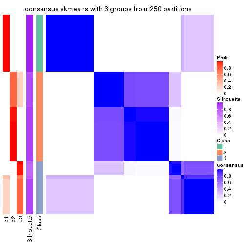
consensus_heatmap(res, k = 4)
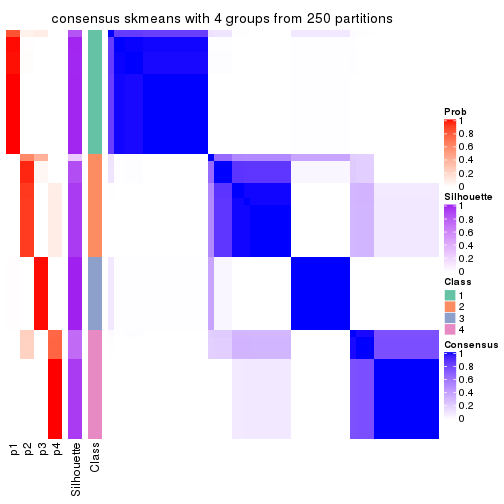
consensus_heatmap(res, k = 5)
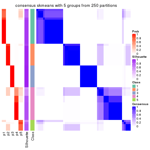
consensus_heatmap(res, k = 6)
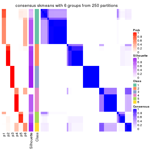
Heatmaps for the membership of samples in all partitions to see how consistent they are:
membership_heatmap(res, k = 2)

membership_heatmap(res, k = 3)
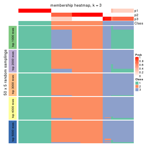
membership_heatmap(res, k = 4)
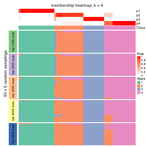
membership_heatmap(res, k = 5)
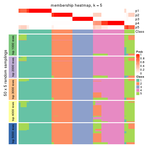
membership_heatmap(res, k = 6)
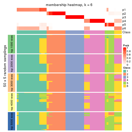
As soon as we have had the classes for columns, we can look for signatures which are significantly different between classes which can be candidate marks for certain classes. Following are the heatmaps for signatures.
Signature heatmaps where rows are scaled:
get_signatures(res, k = 2)

get_signatures(res, k = 3)
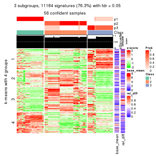
get_signatures(res, k = 4)
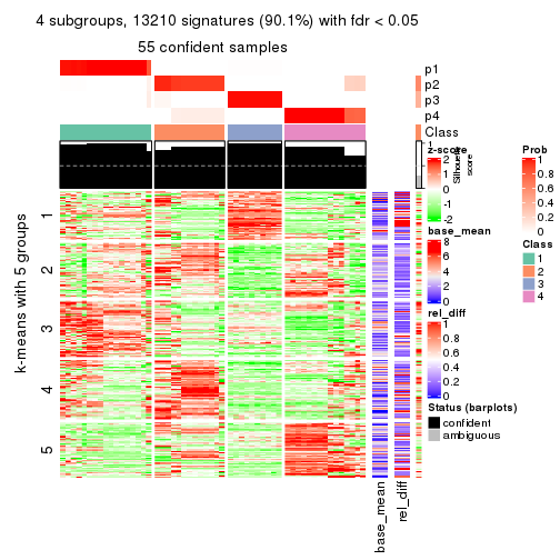
get_signatures(res, k = 5)
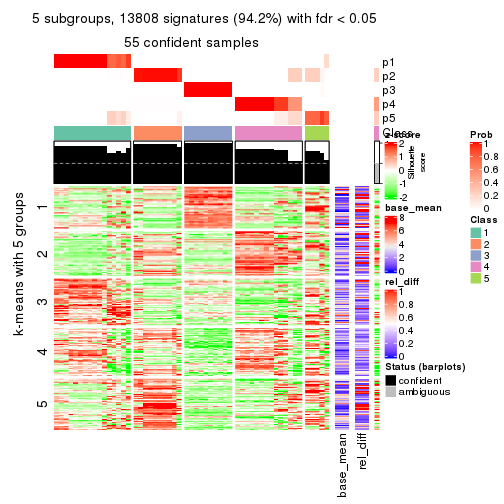
get_signatures(res, k = 6)
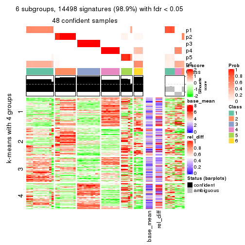
Signature heatmaps where rows are not scaled:
get_signatures(res, k = 2, scale_rows = FALSE)
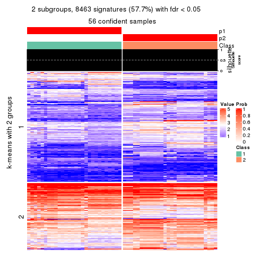
get_signatures(res, k = 3, scale_rows = FALSE)
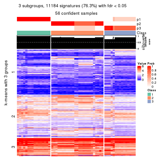
get_signatures(res, k = 4, scale_rows = FALSE)
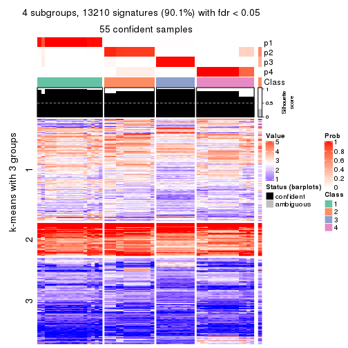
get_signatures(res, k = 5, scale_rows = FALSE)
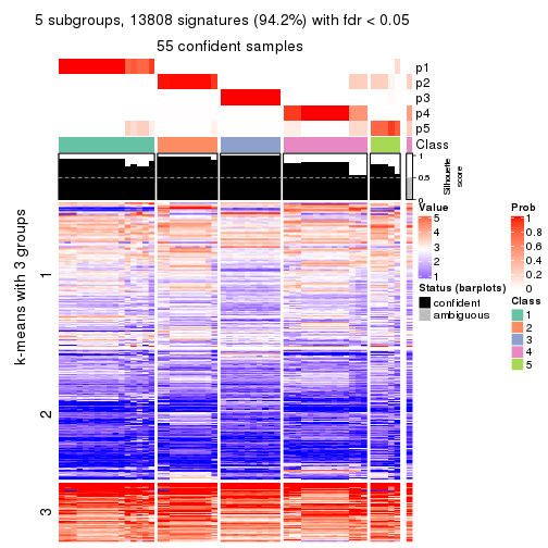
get_signatures(res, k = 6, scale_rows = FALSE)
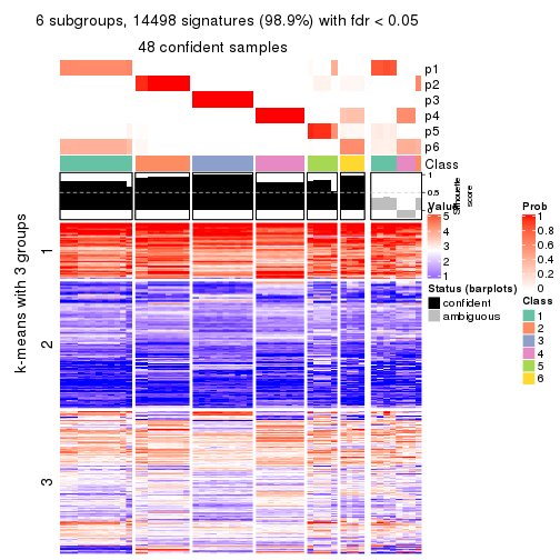
Compare the overlap of signatures from different k:
compare_signatures(res)
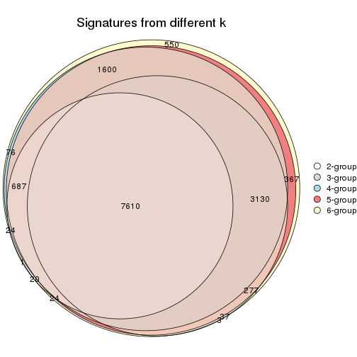
get_signature() returns a data frame invisibly. TO get the list of signatures, the function
call should be assigned to a variable explicitly. In following code, if plot argument is set
to FALSE, no heatmap is plotted while only the differential analysis is performed.
# code only for demonstration
tb = get_signature(res, k = ..., plot = FALSE)
An example of the output of tb is:
#>   which_row         fdr    mean_1    mean_2 scaled_mean_1 scaled_mean_2 km
#> 1        38 0.042760348  8.373488  9.131774    -0.5533452     0.5164555  1
#> 2        40 0.018707592  7.106213  8.469186    -0.6173731     0.5762149  1
#> 3        55 0.019134737 10.221463 11.207825    -0.6159697     0.5749050  1
#> 4        59 0.006059896  5.921854  7.869574    -0.6899429     0.6439467  1
#> 5        60 0.018055526  8.928898 10.211722    -0.6204761     0.5791110  1
#> 6        98 0.009384629 15.714769 14.887706     0.6635654    -0.6193277  2
...
The columns in tb are:
which_row: row indices corresponding to the input matrix.fdr: FDR for the differential test. mean_x: The mean value in group x.scaled_mean_x: The mean value in group x after rows are scaled.km: Row groups if k-means clustering is applied to rows.UMAP plot which shows how samples are separated.
dimension_reduction(res, k = 2, method = "UMAP")
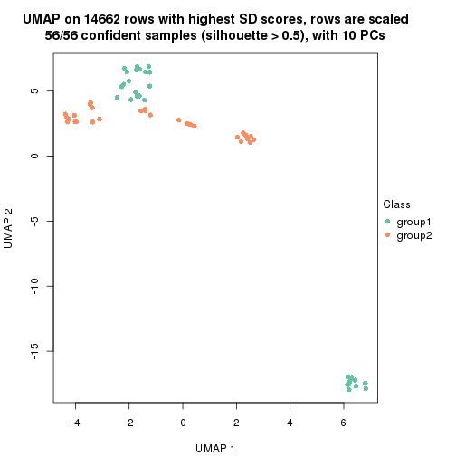
dimension_reduction(res, k = 3, method = "UMAP")
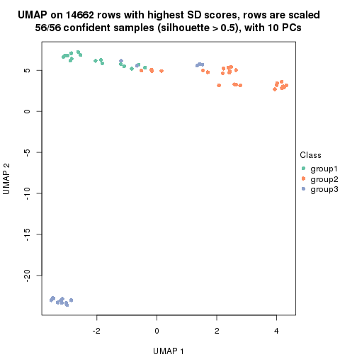
dimension_reduction(res, k = 4, method = "UMAP")
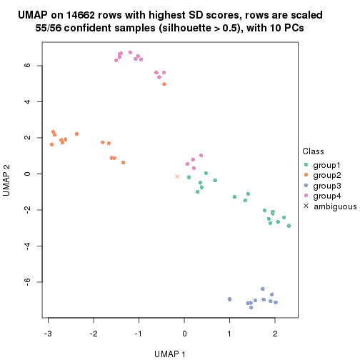
dimension_reduction(res, k = 5, method = "UMAP")
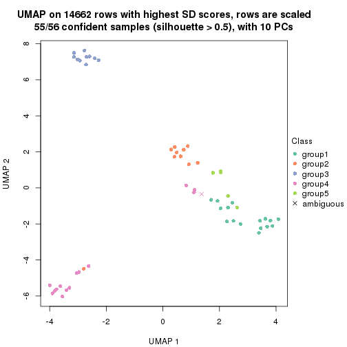
dimension_reduction(res, k = 6, method = "UMAP")
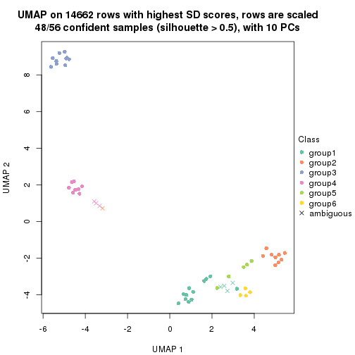
Following heatmap shows how subgroups are split when increasing k:
collect_classes(res)
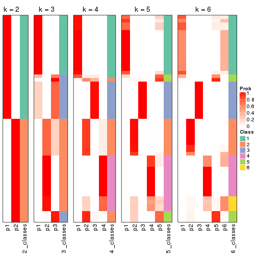
If matrix rows can be associated to genes, consider to use functional_enrichment(res,
...) to perform function enrichment for the signature genes. See this vignette for more detailed explanations.
The object with results only for a single top-value method and a single partition method can be extracted as:
res = res_list["SD", "pam"]
# you can also extract it by
# res = res_list["SD:pam"]
A summary of res and all the functions that can be applied to it:
res
#> A 'ConsensusPartition' object with k = 2, 3, 4, 5, 6.
#>   On a matrix with 14662 rows and 56 columns.
#>   Top rows (1000, 2000, 3000, 4000, 5000) are extracted by 'SD' method.
#>   Subgroups are detected by 'pam' method.
#>   Performed in total 1250 partitions by row resampling.
#>   Best k for subgroups seems to be 6.
#>
#> Following methods can be applied to this 'ConsensusPartition' object:
#>  [1] "cola_report"             "collect_classes"         "collect_plots"
#>  [4] "collect_stats"           "colnames"                "compare_signatures"
#>  [7] "consensus_heatmap"       "dimension_reduction"     "functional_enrichment"
#> [10] "get_anno_col"            "get_anno"                "get_classes"
#> [13] "get_consensus"           "get_matrix"              "get_membership"
#> [16] "get_param"               "get_signatures"          "get_stats"
#> [19] "is_best_k"               "is_stable_k"             "membership_heatmap"
#> [22] "ncol"                    "nrow"                    "plot_ecdf"
#> [25] "rownames"                "select_partition_number" "show"
#> [28] "suggest_best_k"          "test_to_known_factors"
collect_plots() function collects all the plots made from res for all k (number of partitions)
into one single page to provide an easy and fast comparison between different k.
collect_plots(res)
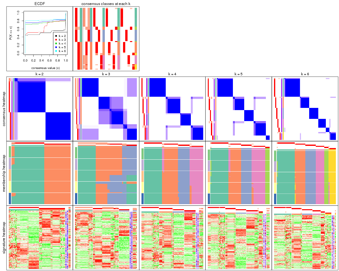
The plots are:
k and the heatmap of
predicted classes for each k.k.k.k.All the plots in panels can be made by individual functions and they are plotted later in this section.
select_partition_number() produces several plots showing different
statistics for choosing “optimized” k. There are following statistics:
k;k, the area increased is defined as \(A_k - A_{k-1}\).The detailed explanations of these statistics can be found in the cola vignette.
Generally speaking, lower PAC score, higher mean silhouette score or higher
concordance corresponds to better partition. Rand index and Jaccard index
measure how similar the current partition is compared to partition with k-1.
If they are too similar, we won't accept k is better than k-1.
select_partition_number(res)
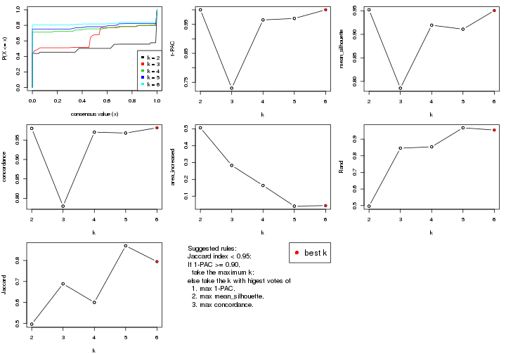
The numeric values for all these statistics can be obtained by get_stats().
get_stats(res)
#>   k 1-PAC mean_silhouette concordance area_increased  Rand Jaccard
#> 2 2 1.000           0.952       0.980         0.5058 0.497   0.497
#> 3 3 0.730           0.786       0.780         0.2827 0.845   0.689
#> 4 4 0.965           0.919       0.970         0.1636 0.854   0.600
#> 5 5 0.970           0.911       0.968         0.0407 0.968   0.870
#> 6 6 1.000           0.951       0.981         0.0440 0.955   0.795
suggest_best_k() suggests the best \(k\) based on these statistics. The rules are as follows:
suggest_best_k(res)
#> [1] 6
#> attr(,"optional")
#> [1] 2 4 5
There is also optional best \(k\) = 2 4 5 that is worth to check.
Following shows the table of the partitions (You need to click the show/hide
code output link to see it). The membership matrix (columns with name p*)
is inferred by
clue::cl_consensus()
function with the SE method. Basically the value in the membership matrix
represents the probability to belong to a certain group. The finall class
label for an item is determined with the group with highest probability it
belongs to.
In get_classes() function, the entropy is calculated from the membership
matrix and the silhouette score is calculated from the consensus matrix.
cbind(get_classes(res, k = 2), get_membership(res, k = 2))
#>           class entropy silhouette    p1    p2
#> SRR073723     1   0.000      0.962 1.000 0.000
#> SRR073724     1   0.000      0.962 1.000 0.000
#> SRR073725     1   0.000      0.962 1.000 0.000
#> SRR073726     2   0.000      1.000 0.000 1.000
#> SRR073727     1   0.000      0.962 1.000 0.000
#> SRR073728     1   0.939      0.488 0.644 0.356
#> SRR073729     1   0.932      0.504 0.652 0.348
#> SRR073730     1   0.952      0.452 0.628 0.372
#> SRR073731     2   0.000      1.000 0.000 1.000
#> SRR073732     2   0.000      1.000 0.000 1.000
#> SRR073733     2   0.000      1.000 0.000 1.000
#> SRR073734     2   0.000      1.000 0.000 1.000
#> SRR073735     2   0.000      1.000 0.000 1.000
#> SRR073736     2   0.000      1.000 0.000 1.000
#> SRR073737     2   0.000      1.000 0.000 1.000
#> SRR073738     1   0.000      0.962 1.000 0.000
#> SRR073739     1   0.000      0.962 1.000 0.000
#> SRR073740     1   0.000      0.962 1.000 0.000
#> SRR073741     1   0.000      0.962 1.000 0.000
#> SRR073742     1   0.000      0.962 1.000 0.000
#> SRR073743     1   0.000      0.962 1.000 0.000
#> SRR073744     1   0.000      0.962 1.000 0.000
#> SRR073745     1   0.000      0.962 1.000 0.000
#> SRR073746     1   0.000      0.962 1.000 0.000
#> SRR073747     1   0.000      0.962 1.000 0.000
#> SRR073748     1   0.000      0.962 1.000 0.000
#> SRR073749     1   0.000      0.962 1.000 0.000
#> SRR073750     1   0.000      0.962 1.000 0.000
#> SRR073751     1   0.295      0.916 0.948 0.052
#> SRR073752     2   0.000      1.000 0.000 1.000
#> SRR073753     2   0.000      1.000 0.000 1.000
#> SRR073754     2   0.000      1.000 0.000 1.000
#> SRR073755     2   0.000      1.000 0.000 1.000
#> SRR073756     2   0.000      1.000 0.000 1.000
#> SRR073758     2   0.000      1.000 0.000 1.000
#> SRR073759     2   0.000      1.000 0.000 1.000
#> SRR073760     2   0.000      1.000 0.000 1.000
#> SRR073761     2   0.000      1.000 0.000 1.000
#> SRR073763     2   0.000      1.000 0.000 1.000
#> SRR073764     2   0.000      1.000 0.000 1.000
#> SRR073765     2   0.000      1.000 0.000 1.000
#> SRR073766     2   0.000      1.000 0.000 1.000
#> SRR073767     2   0.000      1.000 0.000 1.000
#> SRR073768     2   0.000      1.000 0.000 1.000
#> SRR073769     1   0.000      0.962 1.000 0.000
#> SRR073770     1   0.000      0.962 1.000 0.000
#> SRR073771     1   0.000      0.962 1.000 0.000
#> SRR073772     1   0.000      0.962 1.000 0.000
#> SRR073773     1   0.000      0.962 1.000 0.000
#> SRR073774     1   0.000      0.962 1.000 0.000
#> SRR073775     1   0.000      0.962 1.000 0.000
#> SRR073776     1   0.000      0.962 1.000 0.000
#> SRR073777     1   0.000      0.962 1.000 0.000
#> SRR073778     1   0.000      0.962 1.000 0.000
#> SRR073779     2   0.000      1.000 0.000 1.000
#> SRR073780     2   0.000      1.000 0.000 1.000
cbind(get_classes(res, k = 3), get_membership(res, k = 3))
#>           class entropy silhouette    p1    p2    p3
#> SRR073723     1  0.6280      1.000 0.540 0.000 0.460
#> SRR073724     1  0.6280      1.000 0.540 0.000 0.460
#> SRR073725     1  0.6280      1.000 0.540 0.000 0.460
#> SRR073726     2  0.4002      0.761 0.160 0.840 0.000
#> SRR073727     1  0.6280      1.000 0.540 0.000 0.460
#> SRR073728     3  0.7674      0.347 0.044 0.472 0.484
#> SRR073729     3  0.7841      0.344 0.052 0.472 0.476
#> SRR073730     3  0.7584      0.347 0.040 0.472 0.488
#> SRR073731     2  0.0000      0.759 0.000 1.000 0.000
#> SRR073732     2  0.0000      0.759 0.000 1.000 0.000
#> SRR073733     2  0.0000      0.759 0.000 1.000 0.000
#> SRR073734     2  0.0000      0.759 0.000 1.000 0.000
#> SRR073735     2  0.0000      0.759 0.000 1.000 0.000
#> SRR073736     2  0.0000      0.759 0.000 1.000 0.000
#> SRR073737     2  0.0000      0.759 0.000 1.000 0.000
#> SRR073738     1  0.6280      1.000 0.540 0.000 0.460
#> SRR073739     1  0.6280      1.000 0.540 0.000 0.460
#> SRR073740     1  0.6280      1.000 0.540 0.000 0.460
#> SRR073741     1  0.6280      1.000 0.540 0.000 0.460
#> SRR073742     1  0.6280      1.000 0.540 0.000 0.460
#> SRR073743     1  0.6280      1.000 0.540 0.000 0.460
#> SRR073744     1  0.6280      1.000 0.540 0.000 0.460
#> SRR073745     1  0.6280      1.000 0.540 0.000 0.460
#> SRR073746     1  0.6280      1.000 0.540 0.000 0.460
#> SRR073747     1  0.6280      1.000 0.540 0.000 0.460
#> SRR073748     1  0.6280      1.000 0.540 0.000 0.460
#> SRR073749     1  0.6280      1.000 0.540 0.000 0.460
#> SRR073750     1  0.6280      1.000 0.540 0.000 0.460
#> SRR073751     3  0.6274      0.365 0.000 0.456 0.544
#> SRR073752     2  0.0000      0.759 0.000 1.000 0.000
#> SRR073753     2  0.0000      0.759 0.000 1.000 0.000
#> SRR073754     2  0.0592      0.760 0.012 0.988 0.000
#> SRR073755     2  0.6280      0.740 0.460 0.540 0.000
#> SRR073756     2  0.6280      0.740 0.460 0.540 0.000
#> SRR073758     2  0.6280      0.740 0.460 0.540 0.000
#> SRR073759     2  0.0000      0.759 0.000 1.000 0.000
#> SRR073760     2  0.6280      0.740 0.460 0.540 0.000
#> SRR073761     2  0.6280      0.740 0.460 0.540 0.000
#> SRR073763     2  0.6280      0.740 0.460 0.540 0.000
#> SRR073764     2  0.6280      0.740 0.460 0.540 0.000
#> SRR073765     2  0.6280      0.740 0.460 0.540 0.000
#> SRR073766     2  0.6280      0.740 0.460 0.540 0.000
#> SRR073767     2  0.6280      0.740 0.460 0.540 0.000
#> SRR073768     2  0.6280      0.740 0.460 0.540 0.000
#> SRR073769     3  0.0000      0.682 0.000 0.000 1.000
#> SRR073770     3  0.0000      0.682 0.000 0.000 1.000
#> SRR073771     3  0.0000      0.682 0.000 0.000 1.000
#> SRR073772     3  0.0000      0.682 0.000 0.000 1.000
#> SRR073773     3  0.0000      0.682 0.000 0.000 1.000
#> SRR073774     3  0.0000      0.682 0.000 0.000 1.000
#> SRR073775     3  0.0000      0.682 0.000 0.000 1.000
#> SRR073776     3  0.0000      0.682 0.000 0.000 1.000
#> SRR073777     3  0.0000      0.682 0.000 0.000 1.000
#> SRR073778     3  0.0000      0.682 0.000 0.000 1.000
#> SRR073779     2  0.0000      0.759 0.000 1.000 0.000
#> SRR073780     2  0.3941      0.761 0.156 0.844 0.000
cbind(get_classes(res, k = 4), get_membership(res, k = 4))
#>           class entropy silhouette p1    p2    p3    p4
#> SRR073723     1   0.000      1.000  1 0.000 0.000 0.000
#> SRR073724     1   0.000      1.000  1 0.000 0.000 0.000
#> SRR073725     1   0.000      1.000  1 0.000 0.000 0.000
#> SRR073726     4   0.460      0.475  0 0.336 0.000 0.664
#> SRR073727     1   0.000      1.000  1 0.000 0.000 0.000
#> SRR073728     2   0.000      0.933  0 1.000 0.000 0.000
#> SRR073729     2   0.000      0.933  0 1.000 0.000 0.000
#> SRR073730     2   0.000      0.933  0 1.000 0.000 0.000
#> SRR073731     2   0.000      0.933  0 1.000 0.000 0.000
#> SRR073732     2   0.000      0.933  0 1.000 0.000 0.000
#> SRR073733     2   0.000      0.933  0 1.000 0.000 0.000
#> SRR073734     2   0.000      0.933  0 1.000 0.000 0.000
#> SRR073735     2   0.000      0.933  0 1.000 0.000 0.000
#> SRR073736     2   0.000      0.933  0 1.000 0.000 0.000
#> SRR073737     2   0.000      0.933  0 1.000 0.000 0.000
#> SRR073738     1   0.000      1.000  1 0.000 0.000 0.000
#> SRR073739     1   0.000      1.000  1 0.000 0.000 0.000
#> SRR073740     1   0.000      1.000  1 0.000 0.000 0.000
#> SRR073741     1   0.000      1.000  1 0.000 0.000 0.000
#> SRR073742     1   0.000      1.000  1 0.000 0.000 0.000
#> SRR073743     1   0.000      1.000  1 0.000 0.000 0.000
#> SRR073744     1   0.000      1.000  1 0.000 0.000 0.000
#> SRR073745     1   0.000      1.000  1 0.000 0.000 0.000
#> SRR073746     1   0.000      1.000  1 0.000 0.000 0.000
#> SRR073747     1   0.000      1.000  1 0.000 0.000 0.000
#> SRR073748     1   0.000      1.000  1 0.000 0.000 0.000
#> SRR073749     1   0.000      1.000  1 0.000 0.000 0.000
#> SRR073750     1   0.000      1.000  1 0.000 0.000 0.000
#> SRR073751     3   0.322      0.789  0 0.164 0.836 0.000
#> SRR073752     2   0.000      0.933  0 1.000 0.000 0.000
#> SRR073753     2   0.000      0.933  0 1.000 0.000 0.000
#> SRR073754     2   0.493      0.198  0 0.568 0.000 0.432
#> SRR073755     4   0.000      0.937  0 0.000 0.000 1.000
#> SRR073756     4   0.000      0.937  0 0.000 0.000 1.000
#> SRR073758     4   0.000      0.937  0 0.000 0.000 1.000
#> SRR073759     2   0.000      0.933  0 1.000 0.000 0.000
#> SRR073760     4   0.000      0.937  0 0.000 0.000 1.000
#> SRR073761     4   0.000      0.937  0 0.000 0.000 1.000
#> SRR073763     4   0.000      0.937  0 0.000 0.000 1.000
#> SRR073764     4   0.000      0.937  0 0.000 0.000 1.000
#> SRR073765     4   0.000      0.937  0 0.000 0.000 1.000
#> SRR073766     4   0.000      0.937  0 0.000 0.000 1.000
#> SRR073767     4   0.000      0.937  0 0.000 0.000 1.000
#> SRR073768     4   0.000      0.937  0 0.000 0.000 1.000
#> SRR073769     3   0.000      0.982  0 0.000 1.000 0.000
#> SRR073770     3   0.000      0.982  0 0.000 1.000 0.000
#> SRR073771     3   0.000      0.982  0 0.000 1.000 0.000
#> SRR073772     3   0.000      0.982  0 0.000 1.000 0.000
#> SRR073773     3   0.000      0.982  0 0.000 1.000 0.000
#> SRR073774     3   0.000      0.982  0 0.000 1.000 0.000
#> SRR073775     3   0.000      0.982  0 0.000 1.000 0.000
#> SRR073776     3   0.000      0.982  0 0.000 1.000 0.000
#> SRR073777     3   0.000      0.982  0 0.000 1.000 0.000
#> SRR073778     3   0.000      0.982  0 0.000 1.000 0.000
#> SRR073779     2   0.485      0.293  0 0.600 0.000 0.400
#> SRR073780     4   0.458      0.484  0 0.332 0.000 0.668
cbind(get_classes(res, k = 5), get_membership(res, k = 5))
#>           class entropy silhouette    p1    p2 p3    p4    p5
#> SRR073723     1   0.384      0.555 0.692 0.000  0 0.000 0.308
#> SRR073724     1   0.000      0.980 1.000 0.000  0 0.000 0.000
#> SRR073725     1   0.000      0.980 1.000 0.000  0 0.000 0.000
#> SRR073726     4   0.397      0.462 0.000 0.336  0 0.664 0.000
#> SRR073727     1   0.000      0.980 1.000 0.000  0 0.000 0.000
#> SRR073728     5   0.000      1.000 0.000 0.000  0 0.000 1.000
#> SRR073729     5   0.000      1.000 0.000 0.000  0 0.000 1.000
#> SRR073730     5   0.000      1.000 0.000 0.000  0 0.000 1.000
#> SRR073731     2   0.000      0.903 0.000 1.000  0 0.000 0.000
#> SRR073732     2   0.000      0.903 0.000 1.000  0 0.000 0.000
#> SRR073733     2   0.000      0.903 0.000 1.000  0 0.000 0.000
#> SRR073734     2   0.000      0.903 0.000 1.000  0 0.000 0.000
#> SRR073735     2   0.000      0.903 0.000 1.000  0 0.000 0.000
#> SRR073736     2   0.000      0.903 0.000 1.000  0 0.000 0.000
#> SRR073737     2   0.000      0.903 0.000 1.000  0 0.000 0.000
#> SRR073738     1   0.000      0.980 1.000 0.000  0 0.000 0.000
#> SRR073739     1   0.000      0.980 1.000 0.000  0 0.000 0.000
#> SRR073740     1   0.000      0.980 1.000 0.000  0 0.000 0.000
#> SRR073741     1   0.000      0.980 1.000 0.000  0 0.000 0.000
#> SRR073742     1   0.000      0.980 1.000 0.000  0 0.000 0.000
#> SRR073743     1   0.000      0.980 1.000 0.000  0 0.000 0.000
#> SRR073744     1   0.000      0.980 1.000 0.000  0 0.000 0.000
#> SRR073745     1   0.000      0.980 1.000 0.000  0 0.000 0.000
#> SRR073746     1   0.000      0.980 1.000 0.000  0 0.000 0.000
#> SRR073747     1   0.000      0.980 1.000 0.000  0 0.000 0.000
#> SRR073748     1   0.000      0.980 1.000 0.000  0 0.000 0.000
#> SRR073749     1   0.000      0.980 1.000 0.000  0 0.000 0.000
#> SRR073750     1   0.000      0.980 1.000 0.000  0 0.000 0.000
#> SRR073751     5   0.000      1.000 0.000 0.000  0 0.000 1.000
#> SRR073752     2   0.000      0.903 0.000 1.000  0 0.000 0.000
#> SRR073753     2   0.000      0.903 0.000 1.000  0 0.000 0.000
#> SRR073754     2   0.425      0.211 0.000 0.568  0 0.432 0.000
#> SRR073755     4   0.000      0.933 0.000 0.000  0 1.000 0.000
#> SRR073756     4   0.000      0.933 0.000 0.000  0 1.000 0.000
#> SRR073758     4   0.000      0.933 0.000 0.000  0 1.000 0.000
#> SRR073759     2   0.000      0.903 0.000 1.000  0 0.000 0.000
#> SRR073760     4   0.000      0.933 0.000 0.000  0 1.000 0.000
#> SRR073761     4   0.000      0.933 0.000 0.000  0 1.000 0.000
#> SRR073763     4   0.000      0.933 0.000 0.000  0 1.000 0.000
#> SRR073764     4   0.000      0.933 0.000 0.000  0 1.000 0.000
#> SRR073765     4   0.000      0.933 0.000 0.000  0 1.000 0.000
#> SRR073766     4   0.000      0.933 0.000 0.000  0 1.000 0.000
#> SRR073767     4   0.000      0.933 0.000 0.000  0 1.000 0.000
#> SRR073768     4   0.000      0.933 0.000 0.000  0 1.000 0.000
#> SRR073769     3   0.000      1.000 0.000 0.000  1 0.000 0.000
#> SRR073770     3   0.000      1.000 0.000 0.000  1 0.000 0.000
#> SRR073771     3   0.000      1.000 0.000 0.000  1 0.000 0.000
#> SRR073772     3   0.000      1.000 0.000 0.000  1 0.000 0.000
#> SRR073773     3   0.000      1.000 0.000 0.000  1 0.000 0.000
#> SRR073774     3   0.000      1.000 0.000 0.000  1 0.000 0.000
#> SRR073775     3   0.000      1.000 0.000 0.000  1 0.000 0.000
#> SRR073776     3   0.000      1.000 0.000 0.000  1 0.000 0.000
#> SRR073777     3   0.000      1.000 0.000 0.000  1 0.000 0.000
#> SRR073778     3   0.000      1.000 0.000 0.000  1 0.000 0.000
#> SRR073779     2   0.418      0.304 0.000 0.600  0 0.400 0.000
#> SRR073780     4   0.388      0.507 0.000 0.316  0 0.684 0.000
cbind(get_classes(res, k = 6), get_membership(res, k = 6))
#>           class entropy silhouette    p1    p2 p3    p4    p5    p6
#> SRR073723     1   0.345      0.555 0.692 0.000  0 0.000 0.308 0.000
#> SRR073724     1   0.000      0.980 1.000 0.000  0 0.000 0.000 0.000
#> SRR073725     1   0.000      0.980 1.000 0.000  0 0.000 0.000 0.000
#> SRR073726     6   0.000      0.920 0.000 0.000  0 0.000 0.000 1.000
#> SRR073727     1   0.000      0.980 1.000 0.000  0 0.000 0.000 0.000
#> SRR073728     5   0.000      1.000 0.000 0.000  0 0.000 1.000 0.000
#> SRR073729     5   0.000      1.000 0.000 0.000  0 0.000 1.000 0.000
#> SRR073730     5   0.000      1.000 0.000 0.000  0 0.000 1.000 0.000
#> SRR073731     2   0.000      0.959 0.000 1.000  0 0.000 0.000 0.000
#> SRR073732     2   0.000      0.959 0.000 1.000  0 0.000 0.000 0.000
#> SRR073733     2   0.000      0.959 0.000 1.000  0 0.000 0.000 0.000
#> SRR073734     2   0.000      0.959 0.000 1.000  0 0.000 0.000 0.000
#> SRR073735     2   0.000      0.959 0.000 1.000  0 0.000 0.000 0.000
#> SRR073736     2   0.000      0.959 0.000 1.000  0 0.000 0.000 0.000
#> SRR073737     2   0.000      0.959 0.000 1.000  0 0.000 0.000 0.000
#> SRR073738     1   0.000      0.980 1.000 0.000  0 0.000 0.000 0.000
#> SRR073739     1   0.000      0.980 1.000 0.000  0 0.000 0.000 0.000
#> SRR073740     1   0.000      0.980 1.000 0.000  0 0.000 0.000 0.000
#> SRR073741     1   0.000      0.980 1.000 0.000  0 0.000 0.000 0.000
#> SRR073742     1   0.000      0.980 1.000 0.000  0 0.000 0.000 0.000
#> SRR073743     1   0.000      0.980 1.000 0.000  0 0.000 0.000 0.000
#> SRR073744     1   0.000      0.980 1.000 0.000  0 0.000 0.000 0.000
#> SRR073745     1   0.000      0.980 1.000 0.000  0 0.000 0.000 0.000
#> SRR073746     1   0.000      0.980 1.000 0.000  0 0.000 0.000 0.000
#> SRR073747     1   0.000      0.980 1.000 0.000  0 0.000 0.000 0.000
#> SRR073748     1   0.000      0.980 1.000 0.000  0 0.000 0.000 0.000
#> SRR073749     1   0.000      0.980 1.000 0.000  0 0.000 0.000 0.000
#> SRR073750     1   0.000      0.980 1.000 0.000  0 0.000 0.000 0.000
#> SRR073751     5   0.000      1.000 0.000 0.000  0 0.000 1.000 0.000
#> SRR073752     2   0.000      0.959 0.000 1.000  0 0.000 0.000 0.000
#> SRR073753     2   0.000      0.959 0.000 1.000  0 0.000 0.000 0.000
#> SRR073754     6   0.000      0.920 0.000 0.000  0 0.000 0.000 1.000
#> SRR073755     6   0.375      0.332 0.000 0.000  0 0.396 0.000 0.604
#> SRR073756     6   0.000      0.920 0.000 0.000  0 0.000 0.000 1.000
#> SRR073758     6   0.000      0.920 0.000 0.000  0 0.000 0.000 1.000
#> SRR073759     2   0.356      0.506 0.000 0.664  0 0.000 0.000 0.336
#> SRR073760     4   0.000      1.000 0.000 0.000  0 1.000 0.000 0.000
#> SRR073761     4   0.000      1.000 0.000 0.000  0 1.000 0.000 0.000
#> SRR073763     4   0.000      1.000 0.000 0.000  0 1.000 0.000 0.000
#> SRR073764     4   0.000      1.000 0.000 0.000  0 1.000 0.000 0.000
#> SRR073765     4   0.000      1.000 0.000 0.000  0 1.000 0.000 0.000
#> SRR073766     4   0.000      1.000 0.000 0.000  0 1.000 0.000 0.000
#> SRR073767     4   0.000      1.000 0.000 0.000  0 1.000 0.000 0.000
#> SRR073768     4   0.000      1.000 0.000 0.000  0 1.000 0.000 0.000
#> SRR073769     3   0.000      1.000 0.000 0.000  1 0.000 0.000 0.000
#> SRR073770     3   0.000      1.000 0.000 0.000  1 0.000 0.000 0.000
#> SRR073771     3   0.000      1.000 0.000 0.000  1 0.000 0.000 0.000
#> SRR073772     3   0.000      1.000 0.000 0.000  1 0.000 0.000 0.000
#> SRR073773     3   0.000      1.000 0.000 0.000  1 0.000 0.000 0.000
#> SRR073774     3   0.000      1.000 0.000 0.000  1 0.000 0.000 0.000
#> SRR073775     3   0.000      1.000 0.000 0.000  1 0.000 0.000 0.000
#> SRR073776     3   0.000      1.000 0.000 0.000  1 0.000 0.000 0.000
#> SRR073777     3   0.000      1.000 0.000 0.000  1 0.000 0.000 0.000
#> SRR073778     3   0.000      1.000 0.000 0.000  1 0.000 0.000 0.000
#> SRR073779     6   0.000      0.920 0.000 0.000  0 0.000 0.000 1.000
#> SRR073780     6   0.000      0.920 0.000 0.000  0 0.000 0.000 1.000
Heatmaps for the consensus matrix. It visualizes the probability of two samples to be in a same group.
consensus_heatmap(res, k = 2)
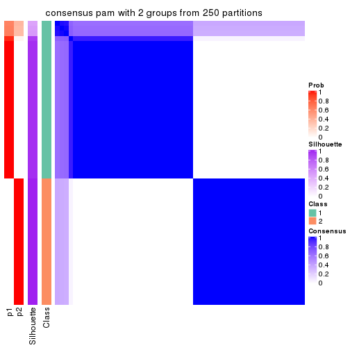
consensus_heatmap(res, k = 3)
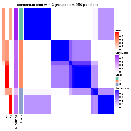
consensus_heatmap(res, k = 4)
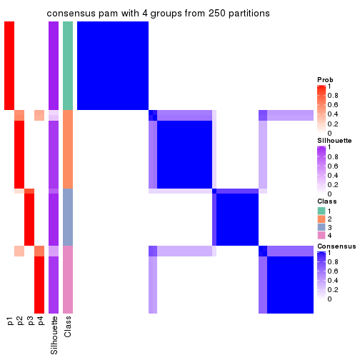
consensus_heatmap(res, k = 5)
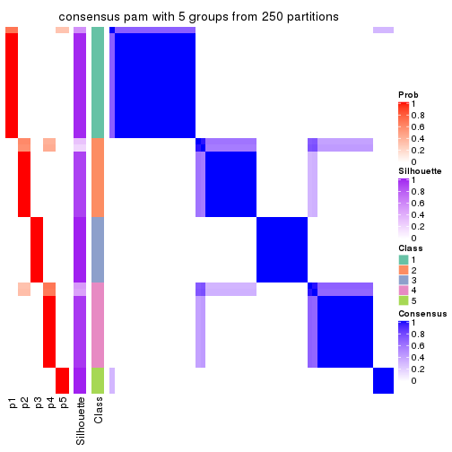
consensus_heatmap(res, k = 6)
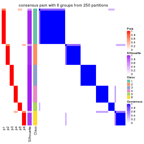
Heatmaps for the membership of samples in all partitions to see how consistent they are:
membership_heatmap(res, k = 2)
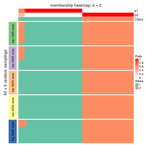
membership_heatmap(res, k = 3)
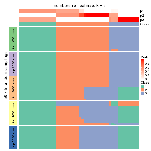
membership_heatmap(res, k = 4)
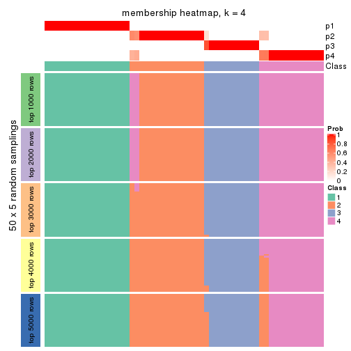
membership_heatmap(res, k = 5)
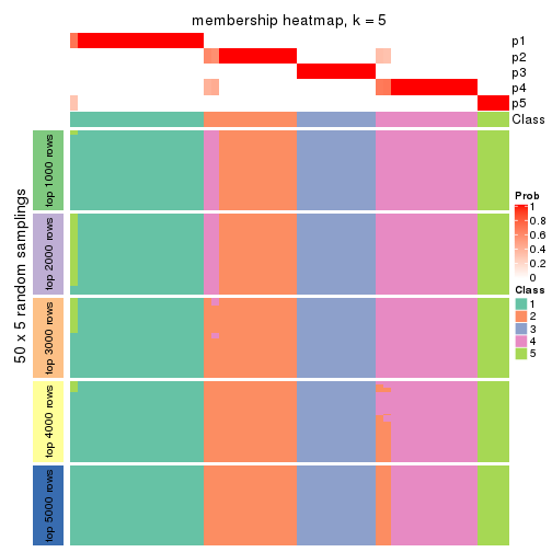
membership_heatmap(res, k = 6)
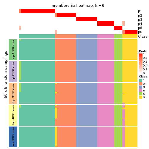
As soon as we have had the classes for columns, we can look for signatures which are significantly different between classes which can be candidate marks for certain classes. Following are the heatmaps for signatures.
Signature heatmaps where rows are scaled:
get_signatures(res, k = 2)
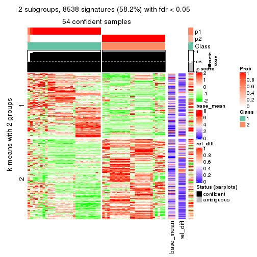
get_signatures(res, k = 3)
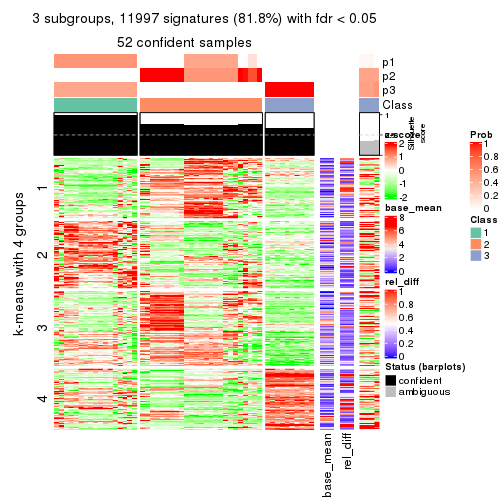
get_signatures(res, k = 4)
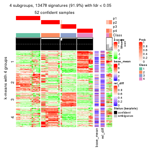
get_signatures(res, k = 5)
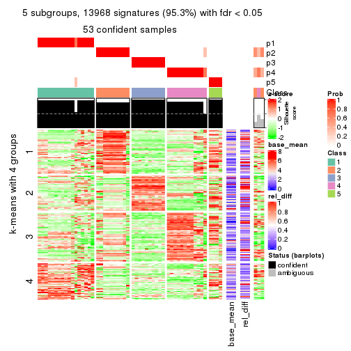
get_signatures(res, k = 6)
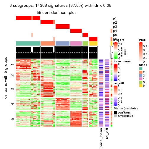
Signature heatmaps where rows are not scaled:
get_signatures(res, k = 2, scale_rows = FALSE)
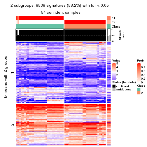
get_signatures(res, k = 3, scale_rows = FALSE)
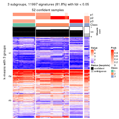
get_signatures(res, k = 4, scale_rows = FALSE)
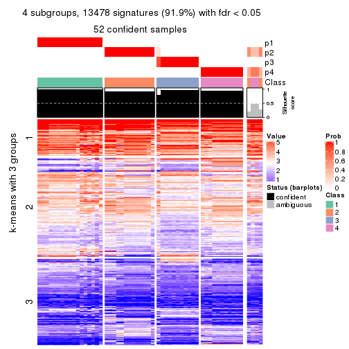
get_signatures(res, k = 5, scale_rows = FALSE)
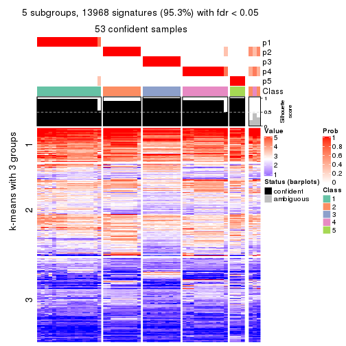
get_signatures(res, k = 6, scale_rows = FALSE)
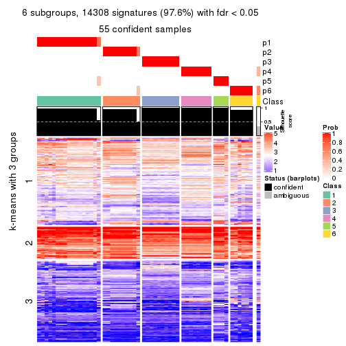
Compare the overlap of signatures from different k:
compare_signatures(res)
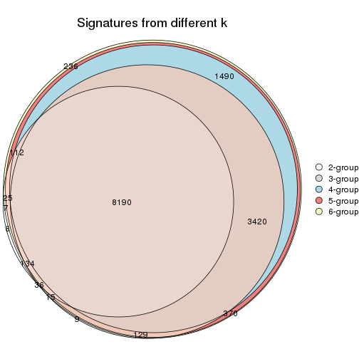
get_signature() returns a data frame invisibly. TO get the list of signatures, the function
call should be assigned to a variable explicitly. In following code, if plot argument is set
to FALSE, no heatmap is plotted while only the differential analysis is performed.
# code only for demonstration
tb = get_signature(res, k = ..., plot = FALSE)
An example of the output of tb is:
#>   which_row         fdr    mean_1    mean_2 scaled_mean_1 scaled_mean_2 km
#> 1        38 0.042760348  8.373488  9.131774    -0.5533452     0.5164555  1
#> 2        40 0.018707592  7.106213  8.469186    -0.6173731     0.5762149  1
#> 3        55 0.019134737 10.221463 11.207825    -0.6159697     0.5749050  1
#> 4        59 0.006059896  5.921854  7.869574    -0.6899429     0.6439467  1
#> 5        60 0.018055526  8.928898 10.211722    -0.6204761     0.5791110  1
#> 6        98 0.009384629 15.714769 14.887706     0.6635654    -0.6193277  2
...
The columns in tb are:
which_row: row indices corresponding to the input matrix.fdr: FDR for the differential test. mean_x: The mean value in group x.scaled_mean_x: The mean value in group x after rows are scaled.km: Row groups if k-means clustering is applied to rows.UMAP plot which shows how samples are separated.
dimension_reduction(res, k = 2, method = "UMAP")
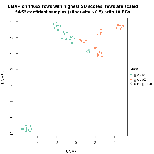
dimension_reduction(res, k = 3, method = "UMAP")
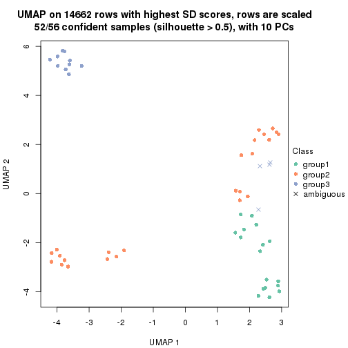
dimension_reduction(res, k = 4, method = "UMAP")

dimension_reduction(res, k = 5, method = "UMAP")

dimension_reduction(res, k = 6, method = "UMAP")

Following heatmap shows how subgroups are split when increasing k:
collect_classes(res)
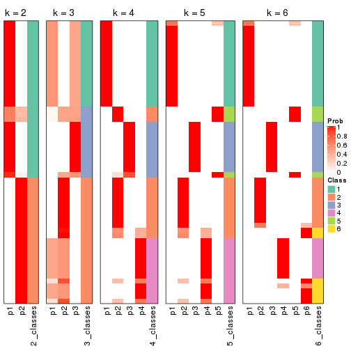
If matrix rows can be associated to genes, consider to use functional_enrichment(res,
...) to perform function enrichment for the signature genes. See this vignette for more detailed explanations.
The object with results only for a single top-value method and a single partition method can be extracted as:
res = res_list["SD", "mclust"]
# you can also extract it by
# res = res_list["SD:mclust"]
A summary of res and all the functions that can be applied to it:
res
#> A 'ConsensusPartition' object with k = 2, 3, 4, 5, 6.
#>   On a matrix with 14662 rows and 56 columns.
#>   Top rows (1000, 2000, 3000, 4000, 5000) are extracted by 'SD' method.
#>   Subgroups are detected by 'mclust' method.
#>   Performed in total 1250 partitions by row resampling.
#>   Best k for subgroups seems to be 4.
#>
#> Following methods can be applied to this 'ConsensusPartition' object:
#>  [1] "cola_report"             "collect_classes"         "collect_plots"
#>  [4] "collect_stats"           "colnames"                "compare_signatures"
#>  [7] "consensus_heatmap"       "dimension_reduction"     "functional_enrichment"
#> [10] "get_anno_col"            "get_anno"                "get_classes"
#> [13] "get_consensus"           "get_matrix"              "get_membership"
#> [16] "get_param"               "get_signatures"          "get_stats"
#> [19] "is_best_k"               "is_stable_k"             "membership_heatmap"
#> [22] "ncol"                    "nrow"                    "plot_ecdf"
#> [25] "rownames"                "select_partition_number" "show"
#> [28] "suggest_best_k"          "test_to_known_factors"
collect_plots() function collects all the plots made from res for all k (number of partitions)
into one single page to provide an easy and fast comparison between different k.
collect_plots(res)
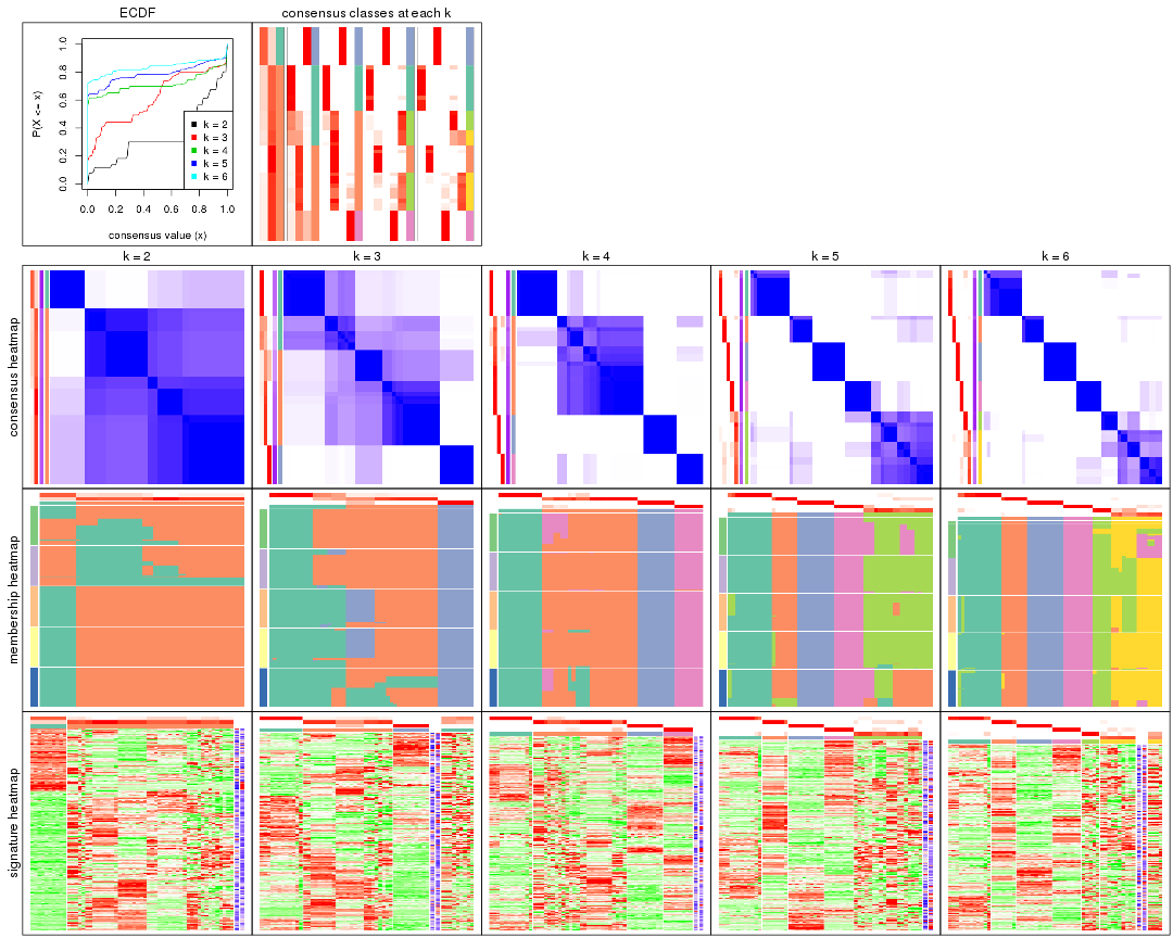
The plots are:
k and the heatmap of
predicted classes for each k.k.k.k.All the plots in panels can be made by individual functions and they are plotted later in this section.
select_partition_number() produces several plots showing different
statistics for choosing “optimized” k. There are following statistics:
k;k, the area increased is defined as \(A_k - A_{k-1}\).The detailed explanations of these statistics can be found in the cola vignette.
Generally speaking, lower PAC score, higher mean silhouette score or higher
concordance corresponds to better partition. Rand index and Jaccard index
measure how similar the current partition is compared to partition with k-1.
If they are too similar, we won't accept k is better than k-1.
select_partition_number(res)
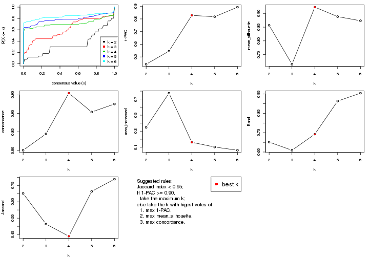
The numeric values for all these statistics can be obtained by get_stats().
get_stats(res)
#>   k 1-PAC mean_silhouette concordance area_increased  Rand Jaccard
#> 2 2 0.442           0.857       0.800         0.3471 0.701   0.701
#> 3 3 0.546           0.715       0.845         0.7745 0.659   0.514
#> 4 4 0.828           0.923       0.955         0.1609 0.742   0.439
#> 5 5 0.817           0.888       0.904         0.1020 0.914   0.713
#> 6 6 0.893           0.873       0.925         0.0617 0.955   0.789
suggest_best_k() suggests the best \(k\) based on these statistics. The rules are as follows:
suggest_best_k(res)
#> [1] 4
Following shows the table of the partitions (You need to click the show/hide
code output link to see it). The membership matrix (columns with name p*)
is inferred by
clue::cl_consensus()
function with the SE method. Basically the value in the membership matrix
represents the probability to belong to a certain group. The finall class
label for an item is determined with the group with highest probability it
belongs to.
In get_classes() function, the entropy is calculated from the membership
matrix and the silhouette score is calculated from the consensus matrix.
cbind(get_classes(res, k = 2), get_membership(res, k = 2))
#>           class entropy silhouette    p1    p2
#> SRR073723     2   0.680      0.821 0.180 0.820
#> SRR073724     2   0.680      0.821 0.180 0.820
#> SRR073725     2   0.753      0.805 0.216 0.784
#> SRR073726     2   0.402      0.829 0.080 0.920
#> SRR073727     2   0.680      0.821 0.180 0.820
#> SRR073728     2   0.584      0.844 0.140 0.860
#> SRR073729     2   0.584      0.844 0.140 0.860
#> SRR073730     2   0.584      0.844 0.140 0.860
#> SRR073731     2   0.000      0.848 0.000 1.000
#> SRR073732     2   0.000      0.848 0.000 1.000
#> SRR073733     2   0.000      0.848 0.000 1.000
#> SRR073734     2   0.000      0.848 0.000 1.000
#> SRR073735     2   0.000      0.848 0.000 1.000
#> SRR073736     2   0.000      0.848 0.000 1.000
#> SRR073737     2   0.000      0.848 0.000 1.000
#> SRR073738     2   0.680      0.821 0.180 0.820
#> SRR073739     2   0.753      0.805 0.216 0.784
#> SRR073740     2   0.753      0.805 0.216 0.784
#> SRR073741     2   0.753      0.805 0.216 0.784
#> SRR073742     2   0.753      0.805 0.216 0.784
#> SRR073743     2   0.753      0.805 0.216 0.784
#> SRR073744     2   0.753      0.805 0.216 0.784
#> SRR073745     2   0.753      0.805 0.216 0.784
#> SRR073746     2   0.753      0.805 0.216 0.784
#> SRR073747     2   0.753      0.805 0.216 0.784
#> SRR073748     2   0.753      0.805 0.216 0.784
#> SRR073749     2   0.753      0.805 0.216 0.784
#> SRR073750     2   0.680      0.821 0.180 0.820
#> SRR073751     2   0.662      0.822 0.172 0.828
#> SRR073752     2   0.373      0.831 0.072 0.928
#> SRR073753     2   0.373      0.831 0.072 0.928
#> SRR073754     2   0.402      0.829 0.080 0.920
#> SRR073755     2   0.402      0.829 0.080 0.920
#> SRR073756     2   0.402      0.829 0.080 0.920
#> SRR073758     2   0.402      0.829 0.080 0.920
#> SRR073759     2   0.402      0.829 0.080 0.920
#> SRR073760     2   0.402      0.829 0.080 0.920
#> SRR073761     2   0.402      0.829 0.080 0.920
#> SRR073763     2   0.402      0.829 0.080 0.920
#> SRR073764     2   0.402      0.829 0.080 0.920
#> SRR073765     2   0.402      0.829 0.080 0.920
#> SRR073766     2   0.402      0.829 0.080 0.920
#> SRR073767     2   0.402      0.829 0.080 0.920
#> SRR073768     2   0.402      0.829 0.080 0.920
#> SRR073769     1   0.738      1.000 0.792 0.208
#> SRR073770     1   0.738      1.000 0.792 0.208
#> SRR073771     1   0.738      1.000 0.792 0.208
#> SRR073772     1   0.738      1.000 0.792 0.208
#> SRR073773     1   0.738      1.000 0.792 0.208
#> SRR073774     1   0.738      1.000 0.792 0.208
#> SRR073775     1   0.738      1.000 0.792 0.208
#> SRR073776     1   0.738      1.000 0.792 0.208
#> SRR073777     1   0.738      1.000 0.792 0.208
#> SRR073778     1   0.738      1.000 0.792 0.208
#> SRR073779     2   0.402      0.829 0.080 0.920
#> SRR073780     2   0.402      0.829 0.080 0.920
cbind(get_classes(res, k = 3), get_membership(res, k = 3))
#>           class entropy silhouette    p1    p2    p3
#> SRR073723     1  0.7346      0.437 0.592 0.368 0.040
#> SRR073724     1  0.6667      0.455 0.616 0.368 0.016
#> SRR073725     1  0.0237      0.750 0.996 0.000 0.004
#> SRR073726     2  0.2625      0.766 0.084 0.916 0.000
#> SRR073727     1  0.7245      0.440 0.596 0.368 0.036
#> SRR073728     1  0.7395      0.318 0.492 0.476 0.032
#> SRR073729     1  0.7395      0.318 0.492 0.476 0.032
#> SRR073730     1  0.7395      0.318 0.492 0.476 0.032
#> SRR073731     2  0.2066      0.774 0.060 0.940 0.000
#> SRR073732     2  0.2066      0.774 0.060 0.940 0.000
#> SRR073733     2  0.2066      0.774 0.060 0.940 0.000
#> SRR073734     2  0.2066      0.774 0.060 0.940 0.000
#> SRR073735     2  0.2066      0.774 0.060 0.940 0.000
#> SRR073736     2  0.2066      0.774 0.060 0.940 0.000
#> SRR073737     2  0.2066      0.774 0.060 0.940 0.000
#> SRR073738     1  0.7245      0.440 0.596 0.368 0.036
#> SRR073739     1  0.0000      0.752 1.000 0.000 0.000
#> SRR073740     1  0.0000      0.752 1.000 0.000 0.000
#> SRR073741     1  0.0000      0.752 1.000 0.000 0.000
#> SRR073742     1  0.0000      0.752 1.000 0.000 0.000
#> SRR073743     1  0.0000      0.752 1.000 0.000 0.000
#> SRR073744     1  0.0000      0.752 1.000 0.000 0.000
#> SRR073745     1  0.0000      0.752 1.000 0.000 0.000
#> SRR073746     1  0.0424      0.749 0.992 0.008 0.000
#> SRR073747     1  0.0000      0.752 1.000 0.000 0.000
#> SRR073748     1  0.0000      0.752 1.000 0.000 0.000
#> SRR073749     1  0.0000      0.752 1.000 0.000 0.000
#> SRR073750     1  0.6209      0.461 0.628 0.368 0.004
#> SRR073751     1  0.7392      0.335 0.500 0.468 0.032
#> SRR073752     2  0.2066      0.774 0.060 0.940 0.000
#> SRR073753     2  0.2066      0.774 0.060 0.940 0.000
#> SRR073754     2  0.2066      0.774 0.060 0.940 0.000
#> SRR073755     2  0.3715      0.724 0.128 0.868 0.004
#> SRR073756     2  0.3715      0.724 0.128 0.868 0.004
#> SRR073758     2  0.3715      0.724 0.128 0.868 0.004
#> SRR073759     2  0.3267      0.750 0.116 0.884 0.000
#> SRR073760     2  0.8291      0.564 0.100 0.580 0.320
#> SRR073761     2  0.8291      0.564 0.100 0.580 0.320
#> SRR073763     2  0.8291      0.564 0.100 0.580 0.320
#> SRR073764     2  0.8291      0.564 0.100 0.580 0.320
#> SRR073765     2  0.8291      0.564 0.100 0.580 0.320
#> SRR073766     2  0.8291      0.564 0.100 0.580 0.320
#> SRR073767     2  0.8291      0.564 0.100 0.580 0.320
#> SRR073768     2  0.8291      0.564 0.100 0.580 0.320
#> SRR073769     3  0.0000      1.000 0.000 0.000 1.000
#> SRR073770     3  0.0000      1.000 0.000 0.000 1.000
#> SRR073771     3  0.0000      1.000 0.000 0.000 1.000
#> SRR073772     3  0.0000      1.000 0.000 0.000 1.000
#> SRR073773     3  0.0000      1.000 0.000 0.000 1.000
#> SRR073774     3  0.0000      1.000 0.000 0.000 1.000
#> SRR073775     3  0.0000      1.000 0.000 0.000 1.000
#> SRR073776     3  0.0000      1.000 0.000 0.000 1.000
#> SRR073777     3  0.0000      1.000 0.000 0.000 1.000
#> SRR073778     3  0.0000      1.000 0.000 0.000 1.000
#> SRR073779     2  0.2066      0.774 0.060 0.940 0.000
#> SRR073780     2  0.2448      0.769 0.076 0.924 0.000
cbind(get_classes(res, k = 4), get_membership(res, k = 4))
#>           class entropy silhouette    p1    p2 p3    p4
#> SRR073723     2  0.2921      0.826 0.140 0.860  0 0.000
#> SRR073724     2  0.3837      0.749 0.224 0.776  0 0.000
#> SRR073725     1  0.0336      0.990 0.992 0.008  0 0.000
#> SRR073726     2  0.2921      0.825 0.000 0.860  0 0.140
#> SRR073727     2  0.3837      0.749 0.224 0.776  0 0.000
#> SRR073728     2  0.0000      0.894 0.000 1.000  0 0.000
#> SRR073729     2  0.0000      0.894 0.000 1.000  0 0.000
#> SRR073730     2  0.0000      0.894 0.000 1.000  0 0.000
#> SRR073731     2  0.0188      0.895 0.000 0.996  0 0.004
#> SRR073732     2  0.0188      0.895 0.000 0.996  0 0.004
#> SRR073733     2  0.0188      0.895 0.000 0.996  0 0.004
#> SRR073734     2  0.0188      0.895 0.000 0.996  0 0.004
#> SRR073735     2  0.0188      0.895 0.000 0.996  0 0.004
#> SRR073736     2  0.0188      0.895 0.000 0.996  0 0.004
#> SRR073737     2  0.0188      0.895 0.000 0.996  0 0.004
#> SRR073738     2  0.3837      0.749 0.224 0.776  0 0.000
#> SRR073739     1  0.0000      0.999 1.000 0.000  0 0.000
#> SRR073740     1  0.0000      0.999 1.000 0.000  0 0.000
#> SRR073741     1  0.0000      0.999 1.000 0.000  0 0.000
#> SRR073742     1  0.0000      0.999 1.000 0.000  0 0.000
#> SRR073743     1  0.0000      0.999 1.000 0.000  0 0.000
#> SRR073744     1  0.0000      0.999 1.000 0.000  0 0.000
#> SRR073745     1  0.0000      0.999 1.000 0.000  0 0.000
#> SRR073746     1  0.0000      0.999 1.000 0.000  0 0.000
#> SRR073747     1  0.0000      0.999 1.000 0.000  0 0.000
#> SRR073748     1  0.0000      0.999 1.000 0.000  0 0.000
#> SRR073749     1  0.0000      0.999 1.000 0.000  0 0.000
#> SRR073750     2  0.3837      0.749 0.224 0.776  0 0.000
#> SRR073751     2  0.1716      0.870 0.064 0.936  0 0.000
#> SRR073752     2  0.0188      0.895 0.000 0.996  0 0.004
#> SRR073753     2  0.0188      0.895 0.000 0.996  0 0.004
#> SRR073754     2  0.2469      0.848 0.000 0.892  0 0.108
#> SRR073755     2  0.4382      0.679 0.000 0.704  0 0.296
#> SRR073756     2  0.4382      0.679 0.000 0.704  0 0.296
#> SRR073758     2  0.4382      0.679 0.000 0.704  0 0.296
#> SRR073759     2  0.0336      0.894 0.000 0.992  0 0.008
#> SRR073760     4  0.0000      1.000 0.000 0.000  0 1.000
#> SRR073761     4  0.0000      1.000 0.000 0.000  0 1.000
#> SRR073763     4  0.0000      1.000 0.000 0.000  0 1.000
#> SRR073764     4  0.0000      1.000 0.000 0.000  0 1.000
#> SRR073765     4  0.0000      1.000 0.000 0.000  0 1.000
#> SRR073766     4  0.0000      1.000 0.000 0.000  0 1.000
#> SRR073767     4  0.0000      1.000 0.000 0.000  0 1.000
#> SRR073768     4  0.0000      1.000 0.000 0.000  0 1.000
#> SRR073769     3  0.0000      1.000 0.000 0.000  1 0.000
#> SRR073770     3  0.0000      1.000 0.000 0.000  1 0.000
#> SRR073771     3  0.0000      1.000 0.000 0.000  1 0.000
#> SRR073772     3  0.0000      1.000 0.000 0.000  1 0.000
#> SRR073773     3  0.0000      1.000 0.000 0.000  1 0.000
#> SRR073774     3  0.0000      1.000 0.000 0.000  1 0.000
#> SRR073775     3  0.0000      1.000 0.000 0.000  1 0.000
#> SRR073776     3  0.0000      1.000 0.000 0.000  1 0.000
#> SRR073777     3  0.0000      1.000 0.000 0.000  1 0.000
#> SRR073778     3  0.0000      1.000 0.000 0.000  1 0.000
#> SRR073779     2  0.2469      0.848 0.000 0.892  0 0.108
#> SRR073780     2  0.2921      0.825 0.000 0.860  0 0.140
cbind(get_classes(res, k = 5), get_membership(res, k = 5))
#>           class entropy silhouette    p1    p2 p3    p4    p5
#> SRR073723     5   0.029      0.771 0.008 0.000  0 0.000 0.992
#> SRR073724     5   0.161      0.743 0.072 0.000  0 0.000 0.928
#> SRR073725     1   0.366      0.697 0.724 0.000  0 0.000 0.276
#> SRR073726     5   0.527      0.761 0.000 0.152  0 0.168 0.680
#> SRR073727     5   0.161      0.743 0.072 0.000  0 0.000 0.928
#> SRR073728     5   0.265      0.802 0.000 0.152  0 0.000 0.848
#> SRR073729     5   0.265      0.802 0.000 0.152  0 0.000 0.848
#> SRR073730     5   0.265      0.802 0.000 0.152  0 0.000 0.848
#> SRR073731     2   0.000      0.957 0.000 1.000  0 0.000 0.000
#> SRR073732     2   0.311      0.666 0.000 0.800  0 0.000 0.200
#> SRR073733     2   0.000      0.957 0.000 1.000  0 0.000 0.000
#> SRR073734     2   0.000      0.957 0.000 1.000  0 0.000 0.000
#> SRR073735     2   0.000      0.957 0.000 1.000  0 0.000 0.000
#> SRR073736     2   0.000      0.957 0.000 1.000  0 0.000 0.000
#> SRR073737     2   0.000      0.957 0.000 1.000  0 0.000 0.000
#> SRR073738     5   0.161      0.743 0.072 0.000  0 0.000 0.928
#> SRR073739     1   0.000      0.960 1.000 0.000  0 0.000 0.000
#> SRR073740     1   0.000      0.960 1.000 0.000  0 0.000 0.000
#> SRR073741     1   0.000      0.960 1.000 0.000  0 0.000 0.000
#> SRR073742     1   0.000      0.960 1.000 0.000  0 0.000 0.000
#> SRR073743     1   0.000      0.960 1.000 0.000  0 0.000 0.000
#> SRR073744     1   0.000      0.960 1.000 0.000  0 0.000 0.000
#> SRR073745     1   0.000      0.960 1.000 0.000  0 0.000 0.000
#> SRR073746     1   0.233      0.834 0.876 0.000  0 0.000 0.124
#> SRR073747     1   0.000      0.960 1.000 0.000  0 0.000 0.000
#> SRR073748     1   0.000      0.960 1.000 0.000  0 0.000 0.000
#> SRR073749     1   0.000      0.960 1.000 0.000  0 0.000 0.000
#> SRR073750     5   0.161      0.743 0.072 0.000  0 0.000 0.928
#> SRR073751     5   0.281      0.802 0.004 0.152  0 0.000 0.844
#> SRR073752     5   0.334      0.747 0.000 0.228  0 0.000 0.772
#> SRR073753     5   0.334      0.747 0.000 0.228  0 0.000 0.772
#> SRR073754     5   0.501      0.776 0.000 0.152  0 0.140 0.708
#> SRR073755     5   0.398      0.628 0.000 0.000  0 0.340 0.660
#> SRR073756     5   0.398      0.628 0.000 0.000  0 0.340 0.660
#> SRR073758     5   0.398      0.628 0.000 0.000  0 0.340 0.660
#> SRR073759     5   0.281      0.803 0.000 0.152  0 0.004 0.844
#> SRR073760     4   0.000      1.000 0.000 0.000  0 1.000 0.000
#> SRR073761     4   0.000      1.000 0.000 0.000  0 1.000 0.000
#> SRR073763     4   0.000      1.000 0.000 0.000  0 1.000 0.000
#> SRR073764     4   0.000      1.000 0.000 0.000  0 1.000 0.000
#> SRR073765     4   0.000      1.000 0.000 0.000  0 1.000 0.000
#> SRR073766     4   0.000      1.000 0.000 0.000  0 1.000 0.000
#> SRR073767     4   0.000      1.000 0.000 0.000  0 1.000 0.000
#> SRR073768     4   0.000      1.000 0.000 0.000  0 1.000 0.000
#> SRR073769     3   0.000      1.000 0.000 0.000  1 0.000 0.000
#> SRR073770     3   0.000      1.000 0.000 0.000  1 0.000 0.000
#> SRR073771     3   0.000      1.000 0.000 0.000  1 0.000 0.000
#> SRR073772     3   0.000      1.000 0.000 0.000  1 0.000 0.000
#> SRR073773     3   0.000      1.000 0.000 0.000  1 0.000 0.000
#> SRR073774     3   0.000      1.000 0.000 0.000  1 0.000 0.000
#> SRR073775     3   0.000      1.000 0.000 0.000  1 0.000 0.000
#> SRR073776     3   0.000      1.000 0.000 0.000  1 0.000 0.000
#> SRR073777     3   0.000      1.000 0.000 0.000  1 0.000 0.000
#> SRR073778     3   0.000      1.000 0.000 0.000  1 0.000 0.000
#> SRR073779     5   0.501      0.776 0.000 0.152  0 0.140 0.708
#> SRR073780     5   0.527      0.761 0.000 0.152  0 0.168 0.680
cbind(get_classes(res, k = 6), get_membership(res, k = 6))
#>           class entropy silhouette    p1    p2 p3    p4    p5    p6
#> SRR073723     5  0.0458      0.974 0.000 0.000  0 0.000 0.984 0.016
#> SRR073724     5  0.0000      0.994 0.000 0.000  0 0.000 1.000 0.000
#> SRR073725     1  0.2996      0.730 0.772 0.000  0 0.000 0.228 0.000
#> SRR073726     6  0.2092      0.710 0.000 0.000  0 0.124 0.000 0.876
#> SRR073727     5  0.0000      0.994 0.000 0.000  0 0.000 1.000 0.000
#> SRR073728     6  0.3817      0.369 0.000 0.000  0 0.000 0.432 0.568
#> SRR073729     6  0.3817      0.369 0.000 0.000  0 0.000 0.432 0.568
#> SRR073730     6  0.3817      0.369 0.000 0.000  0 0.000 0.432 0.568
#> SRR073731     2  0.0000      0.980 0.000 1.000  0 0.000 0.000 0.000
#> SRR073732     2  0.1714      0.876 0.000 0.908  0 0.000 0.000 0.092
#> SRR073733     2  0.0000      0.980 0.000 1.000  0 0.000 0.000 0.000
#> SRR073734     2  0.0000      0.980 0.000 1.000  0 0.000 0.000 0.000
#> SRR073735     2  0.0000      0.980 0.000 1.000  0 0.000 0.000 0.000
#> SRR073736     2  0.0000      0.980 0.000 1.000  0 0.000 0.000 0.000
#> SRR073737     2  0.0000      0.980 0.000 1.000  0 0.000 0.000 0.000
#> SRR073738     5  0.0000      0.994 0.000 0.000  0 0.000 1.000 0.000
#> SRR073739     1  0.0000      0.951 1.000 0.000  0 0.000 0.000 0.000
#> SRR073740     1  0.0000      0.951 1.000 0.000  0 0.000 0.000 0.000
#> SRR073741     1  0.0000      0.951 1.000 0.000  0 0.000 0.000 0.000
#> SRR073742     1  0.0000      0.951 1.000 0.000  0 0.000 0.000 0.000
#> SRR073743     1  0.0000      0.951 1.000 0.000  0 0.000 0.000 0.000
#> SRR073744     1  0.0000      0.951 1.000 0.000  0 0.000 0.000 0.000
#> SRR073745     1  0.0000      0.951 1.000 0.000  0 0.000 0.000 0.000
#> SRR073746     1  0.2969      0.702 0.776 0.000  0 0.000 0.224 0.000
#> SRR073747     1  0.0632      0.944 0.976 0.000  0 0.000 0.024 0.000
#> SRR073748     1  0.0632      0.944 0.976 0.000  0 0.000 0.024 0.000
#> SRR073749     1  0.0632      0.944 0.976 0.000  0 0.000 0.024 0.000
#> SRR073750     5  0.0000      0.994 0.000 0.000  0 0.000 1.000 0.000
#> SRR073751     6  0.3828      0.359 0.000 0.000  0 0.000 0.440 0.560
#> SRR073752     6  0.4012      0.622 0.000 0.076  0 0.000 0.176 0.748
#> SRR073753     6  0.4012      0.622 0.000 0.076  0 0.000 0.176 0.748
#> SRR073754     6  0.2527      0.708 0.000 0.004  0 0.084 0.032 0.880
#> SRR073755     6  0.2597      0.690 0.000 0.000  0 0.176 0.000 0.824
#> SRR073756     6  0.2597      0.690 0.000 0.000  0 0.176 0.000 0.824
#> SRR073758     6  0.2597      0.690 0.000 0.000  0 0.176 0.000 0.824
#> SRR073759     6  0.2378      0.654 0.000 0.000  0 0.000 0.152 0.848
#> SRR073760     4  0.0000      1.000 0.000 0.000  0 1.000 0.000 0.000
#> SRR073761     4  0.0000      1.000 0.000 0.000  0 1.000 0.000 0.000
#> SRR073763     4  0.0000      1.000 0.000 0.000  0 1.000 0.000 0.000
#> SRR073764     4  0.0000      1.000 0.000 0.000  0 1.000 0.000 0.000
#> SRR073765     4  0.0000      1.000 0.000 0.000  0 1.000 0.000 0.000
#> SRR073766     4  0.0000      1.000 0.000 0.000  0 1.000 0.000 0.000
#> SRR073767     4  0.0000      1.000 0.000 0.000  0 1.000 0.000 0.000
#> SRR073768     4  0.0000      1.000 0.000 0.000  0 1.000 0.000 0.000
#> SRR073769     3  0.0000      1.000 0.000 0.000  1 0.000 0.000 0.000
#> SRR073770     3  0.0000      1.000 0.000 0.000  1 0.000 0.000 0.000
#> SRR073771     3  0.0000      1.000 0.000 0.000  1 0.000 0.000 0.000
#> SRR073772     3  0.0000      1.000 0.000 0.000  1 0.000 0.000 0.000
#> SRR073773     3  0.0000      1.000 0.000 0.000  1 0.000 0.000 0.000
#> SRR073774     3  0.0000      1.000 0.000 0.000  1 0.000 0.000 0.000
#> SRR073775     3  0.0000      1.000 0.000 0.000  1 0.000 0.000 0.000
#> SRR073776     3  0.0000      1.000 0.000 0.000  1 0.000 0.000 0.000
#> SRR073777     3  0.0000      1.000 0.000 0.000  1 0.000 0.000 0.000
#> SRR073778     3  0.0000      1.000 0.000 0.000  1 0.000 0.000 0.000
#> SRR073779     6  0.2384      0.708 0.000 0.000  0 0.084 0.032 0.884
#> SRR073780     6  0.2092      0.710 0.000 0.000  0 0.124 0.000 0.876
Heatmaps for the consensus matrix. It visualizes the probability of two samples to be in a same group.
consensus_heatmap(res, k = 2)
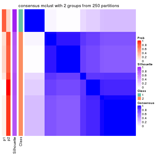
consensus_heatmap(res, k = 3)
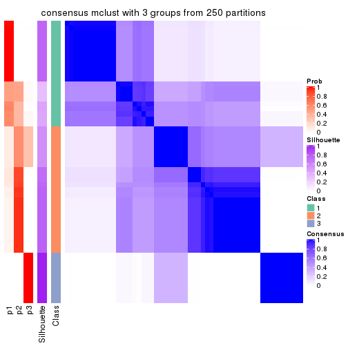
consensus_heatmap(res, k = 4)
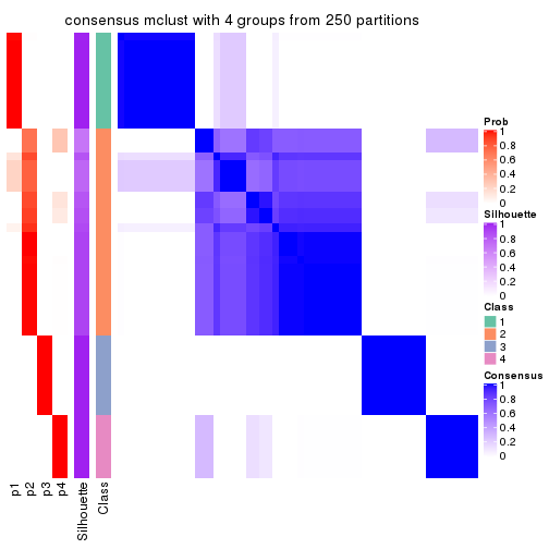
consensus_heatmap(res, k = 5)
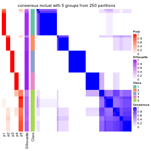
consensus_heatmap(res, k = 6)
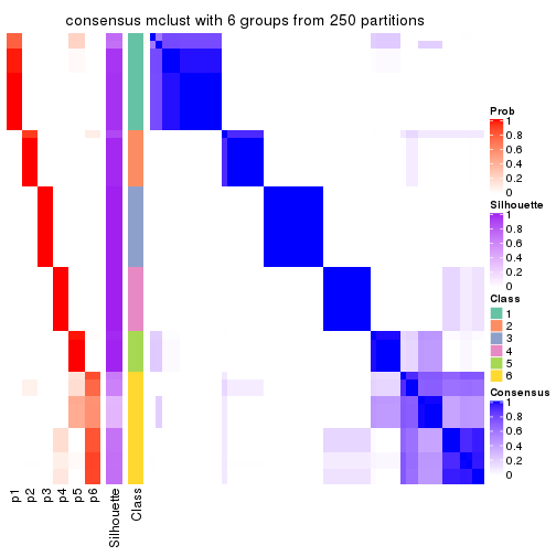
Heatmaps for the membership of samples in all partitions to see how consistent they are:
membership_heatmap(res, k = 2)
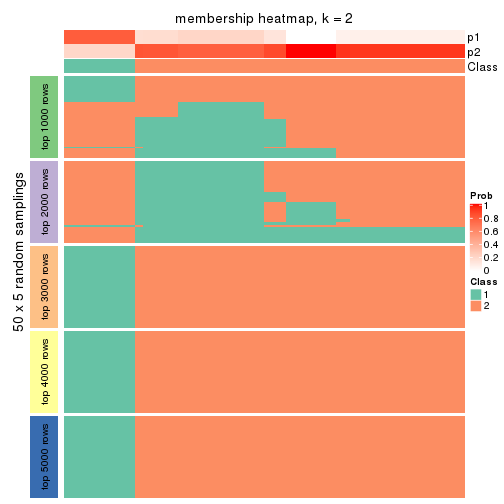
membership_heatmap(res, k = 3)
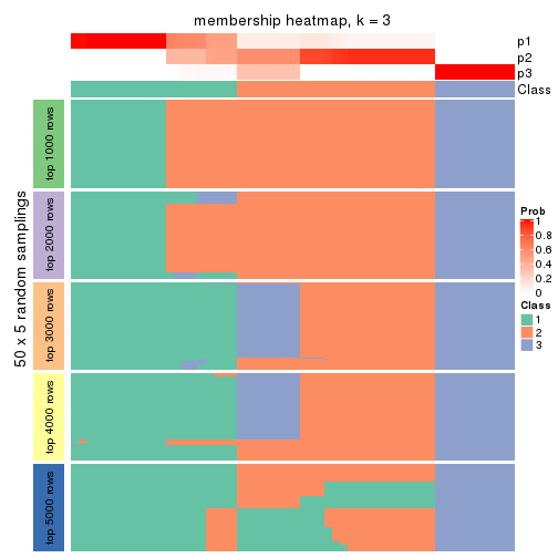
membership_heatmap(res, k = 4)
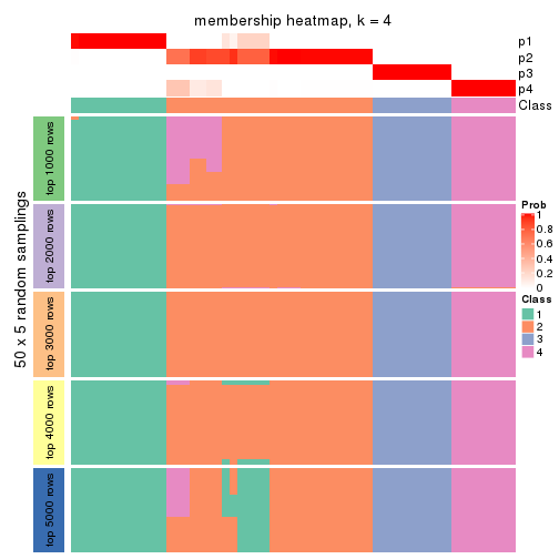
membership_heatmap(res, k = 5)

membership_heatmap(res, k = 6)
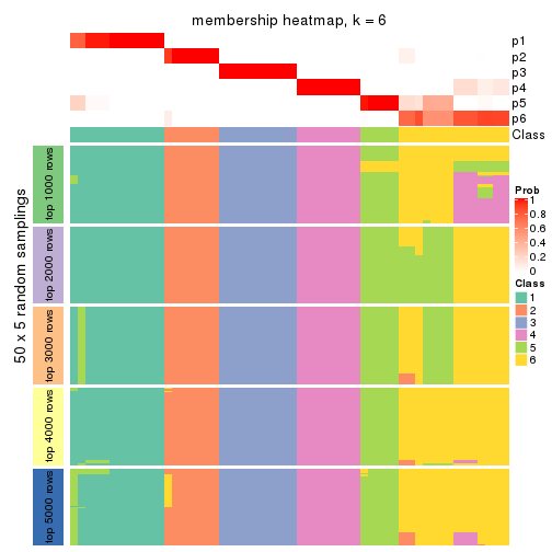
As soon as we have had the classes for columns, we can look for signatures which are significantly different between classes which can be candidate marks for certain classes. Following are the heatmaps for signatures.
Signature heatmaps where rows are scaled:
get_signatures(res, k = 2)
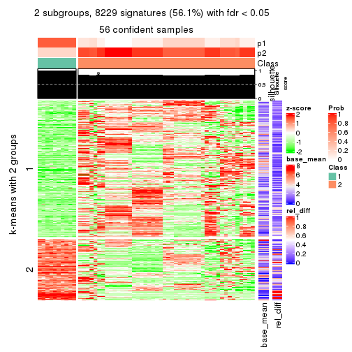
get_signatures(res, k = 3)
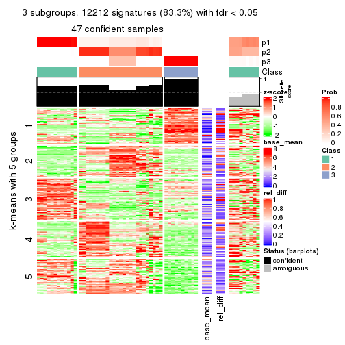
get_signatures(res, k = 4)
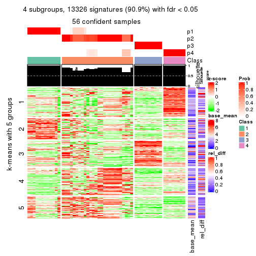
get_signatures(res, k = 5)
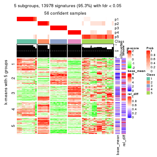
get_signatures(res, k = 6)
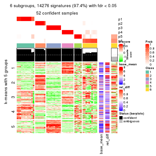
Signature heatmaps where rows are not scaled:
get_signatures(res, k = 2, scale_rows = FALSE)
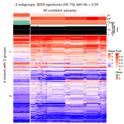
get_signatures(res, k = 3, scale_rows = FALSE)
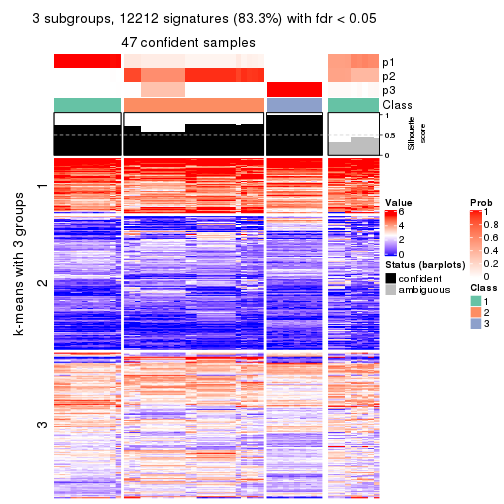
get_signatures(res, k = 4, scale_rows = FALSE)
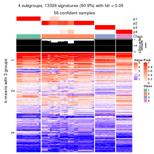
get_signatures(res, k = 5, scale_rows = FALSE)
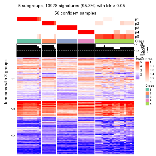
get_signatures(res, k = 6, scale_rows = FALSE)
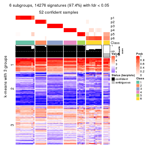
Compare the overlap of signatures from different k:
compare_signatures(res)
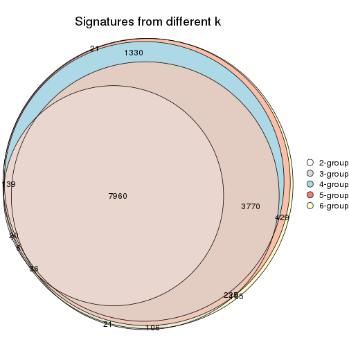
get_signature() returns a data frame invisibly. TO get the list of signatures, the function
call should be assigned to a variable explicitly. In following code, if plot argument is set
to FALSE, no heatmap is plotted while only the differential analysis is performed.
# code only for demonstration
tb = get_signature(res, k = ..., plot = FALSE)
An example of the output of tb is:
#>   which_row         fdr    mean_1    mean_2 scaled_mean_1 scaled_mean_2 km
#> 1        38 0.042760348  8.373488  9.131774    -0.5533452     0.5164555  1
#> 2        40 0.018707592  7.106213  8.469186    -0.6173731     0.5762149  1
#> 3        55 0.019134737 10.221463 11.207825    -0.6159697     0.5749050  1
#> 4        59 0.006059896  5.921854  7.869574    -0.6899429     0.6439467  1
#> 5        60 0.018055526  8.928898 10.211722    -0.6204761     0.5791110  1
#> 6        98 0.009384629 15.714769 14.887706     0.6635654    -0.6193277  2
...
The columns in tb are:
which_row: row indices corresponding to the input matrix.fdr: FDR for the differential test. mean_x: The mean value in group x.scaled_mean_x: The mean value in group x after rows are scaled.km: Row groups if k-means clustering is applied to rows.UMAP plot which shows how samples are separated.
dimension_reduction(res, k = 2, method = "UMAP")

dimension_reduction(res, k = 3, method = "UMAP")
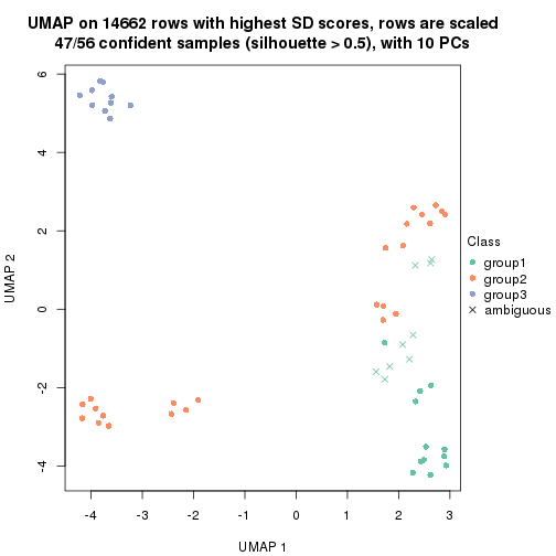
dimension_reduction(res, k = 4, method = "UMAP")
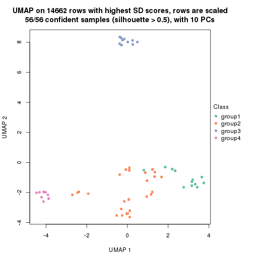
dimension_reduction(res, k = 5, method = "UMAP")
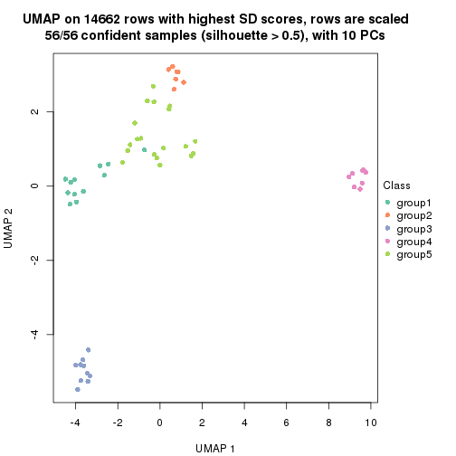
dimension_reduction(res, k = 6, method = "UMAP")
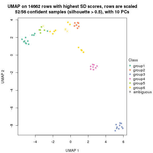
Following heatmap shows how subgroups are split when increasing k:
collect_classes(res)
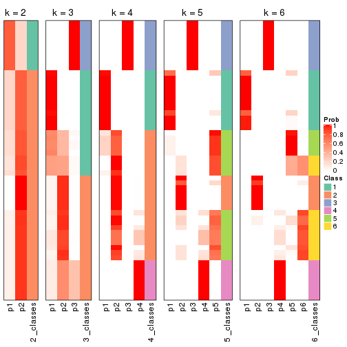
If matrix rows can be associated to genes, consider to use functional_enrichment(res,
...) to perform function enrichment for the signature genes. See this vignette for more detailed explanations.
The object with results only for a single top-value method and a single partition method can be extracted as:
res = res_list["SD", "NMF"]
# you can also extract it by
# res = res_list["SD:NMF"]
A summary of res and all the functions that can be applied to it:
res
#> A 'ConsensusPartition' object with k = 2, 3, 4, 5, 6.
#>   On a matrix with 14662 rows and 56 columns.
#>   Top rows (1000, 2000, 3000, 4000, 5000) are extracted by 'SD' method.
#>   Subgroups are detected by 'NMF' method.
#>   Performed in total 1250 partitions by row resampling.
#>   Best k for subgroups seems to be 6.
#>
#> Following methods can be applied to this 'ConsensusPartition' object:
#>  [1] "cola_report"             "collect_classes"         "collect_plots"
#>  [4] "collect_stats"           "colnames"                "compare_signatures"
#>  [7] "consensus_heatmap"       "dimension_reduction"     "functional_enrichment"
#> [10] "get_anno_col"            "get_anno"                "get_classes"
#> [13] "get_consensus"           "get_matrix"              "get_membership"
#> [16] "get_param"               "get_signatures"          "get_stats"
#> [19] "is_best_k"               "is_stable_k"             "membership_heatmap"
#> [22] "ncol"                    "nrow"                    "plot_ecdf"
#> [25] "rownames"                "select_partition_number" "show"
#> [28] "suggest_best_k"          "test_to_known_factors"
collect_plots() function collects all the plots made from res for all k (number of partitions)
into one single page to provide an easy and fast comparison between different k.
collect_plots(res)
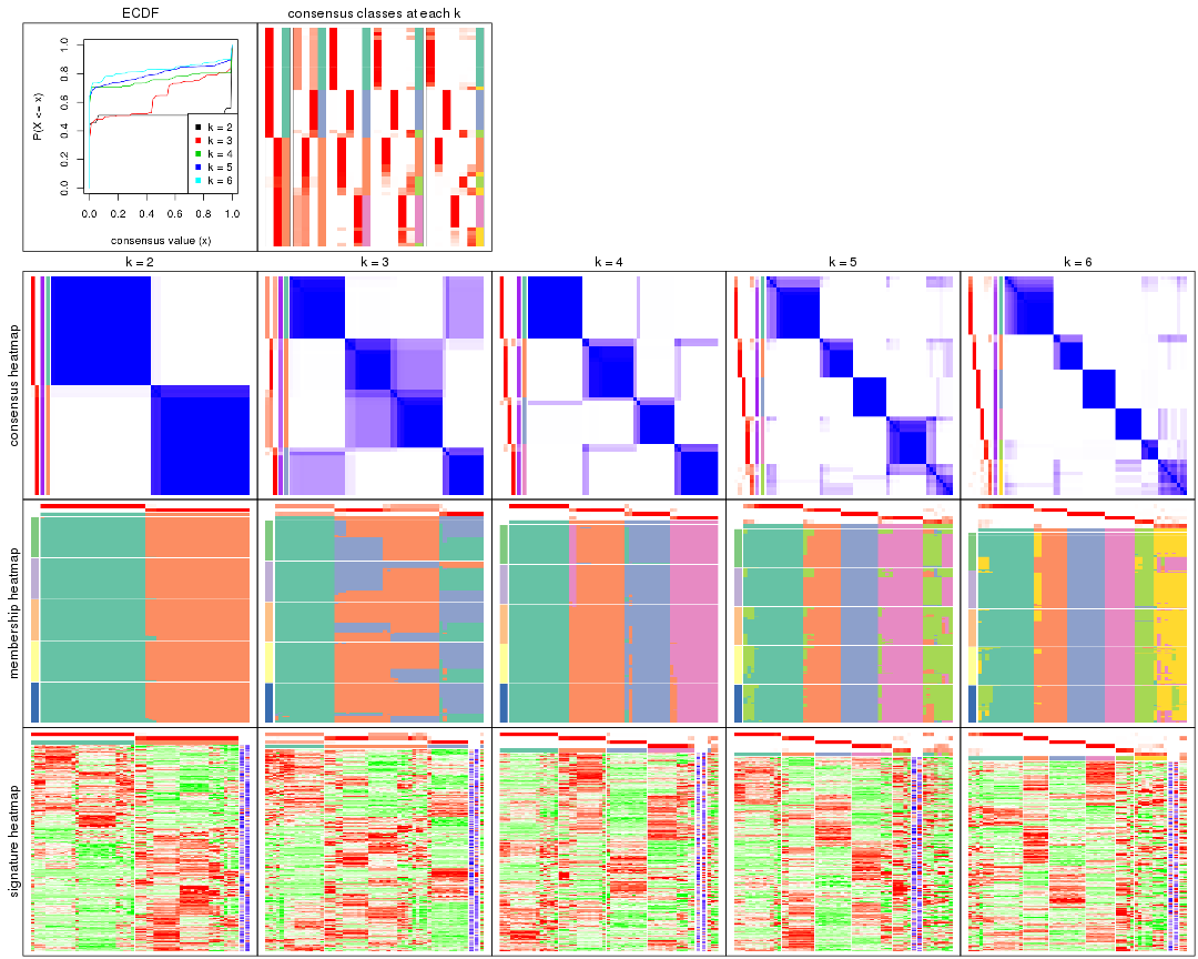
The plots are:
k and the heatmap of
predicted classes for each k.k.k.k.All the plots in panels can be made by individual functions and they are plotted later in this section.
select_partition_number() produces several plots showing different
statistics for choosing “optimized” k. There are following statistics:
k;k, the area increased is defined as \(A_k - A_{k-1}\).The detailed explanations of these statistics can be found in the cola vignette.
Generally speaking, lower PAC score, higher mean silhouette score or higher
concordance corresponds to better partition. Rand index and Jaccard index
measure how similar the current partition is compared to partition with k-1.
If they are too similar, we won't accept k is better than k-1.
select_partition_number(res)

The numeric values for all these statistics can be obtained by get_stats().
get_stats(res)
#>   k 1-PAC mean_silhouette concordance area_increased  Rand Jaccard
#> 2 2 1.000           0.995       0.997         0.5093 0.491   0.491
#> 3 3 0.734           0.851       0.768         0.2531 0.875   0.746
#> 4 4 0.946           0.901       0.962         0.1856 0.873   0.654
#> 5 5 0.882           0.800       0.914         0.0579 0.936   0.744
#> 6 6 0.907           0.877       0.929         0.0372 0.936   0.704
suggest_best_k() suggests the best \(k\) based on these statistics. The rules are as follows:
suggest_best_k(res)
#> [1] 6
#> attr(,"optional")
#> [1] 2 4
There is also optional best \(k\) = 2 4 that is worth to check.
Following shows the table of the partitions (You need to click the show/hide
code output link to see it). The membership matrix (columns with name p*)
is inferred by
clue::cl_consensus()
function with the SE method. Basically the value in the membership matrix
represents the probability to belong to a certain group. The finall class
label for an item is determined with the group with highest probability it
belongs to.
In get_classes() function, the entropy is calculated from the membership
matrix and the silhouette score is calculated from the consensus matrix.
cbind(get_classes(res, k = 2), get_membership(res, k = 2))
#>           class entropy silhouette    p1    p2
#> SRR073723     1  0.0000      1.000 1.000 0.000
#> SRR073724     1  0.0000      1.000 1.000 0.000
#> SRR073725     1  0.0000      1.000 1.000 0.000
#> SRR073726     2  0.0000      0.994 0.000 1.000
#> SRR073727     1  0.0000      1.000 1.000 0.000
#> SRR073728     2  0.2948      0.949 0.052 0.948
#> SRR073729     2  0.2603      0.956 0.044 0.956
#> SRR073730     2  0.3274      0.941 0.060 0.940
#> SRR073731     2  0.0000      0.994 0.000 1.000
#> SRR073732     2  0.0000      0.994 0.000 1.000
#> SRR073733     2  0.0000      0.994 0.000 1.000
#> SRR073734     2  0.0000      0.994 0.000 1.000
#> SRR073735     2  0.0000      0.994 0.000 1.000
#> SRR073736     2  0.0000      0.994 0.000 1.000
#> SRR073737     2  0.0000      0.994 0.000 1.000
#> SRR073738     1  0.0000      1.000 1.000 0.000
#> SRR073739     1  0.0000      1.000 1.000 0.000
#> SRR073740     1  0.0000      1.000 1.000 0.000
#> SRR073741     1  0.0000      1.000 1.000 0.000
#> SRR073742     1  0.0000      1.000 1.000 0.000
#> SRR073743     1  0.0000      1.000 1.000 0.000
#> SRR073744     1  0.0000      1.000 1.000 0.000
#> SRR073745     1  0.0000      1.000 1.000 0.000
#> SRR073746     1  0.0000      1.000 1.000 0.000
#> SRR073747     1  0.0000      1.000 1.000 0.000
#> SRR073748     1  0.0000      1.000 1.000 0.000
#> SRR073749     1  0.0000      1.000 1.000 0.000
#> SRR073750     1  0.0000      1.000 1.000 0.000
#> SRR073751     1  0.0376      0.996 0.996 0.004
#> SRR073752     2  0.0000      0.994 0.000 1.000
#> SRR073753     2  0.0000      0.994 0.000 1.000
#> SRR073754     2  0.0000      0.994 0.000 1.000
#> SRR073755     2  0.0000      0.994 0.000 1.000
#> SRR073756     2  0.0000      0.994 0.000 1.000
#> SRR073758     2  0.0000      0.994 0.000 1.000
#> SRR073759     2  0.0000      0.994 0.000 1.000
#> SRR073760     2  0.0000      0.994 0.000 1.000
#> SRR073761     2  0.0000      0.994 0.000 1.000
#> SRR073763     2  0.0000      0.994 0.000 1.000
#> SRR073764     2  0.0000      0.994 0.000 1.000
#> SRR073765     2  0.0000      0.994 0.000 1.000
#> SRR073766     2  0.0000      0.994 0.000 1.000
#> SRR073767     2  0.0000      0.994 0.000 1.000
#> SRR073768     2  0.0000      0.994 0.000 1.000
#> SRR073769     1  0.0000      1.000 1.000 0.000
#> SRR073770     1  0.0000      1.000 1.000 0.000
#> SRR073771     1  0.0000      1.000 1.000 0.000
#> SRR073772     1  0.0000      1.000 1.000 0.000
#> SRR073773     1  0.0000      1.000 1.000 0.000
#> SRR073774     1  0.0000      1.000 1.000 0.000
#> SRR073775     1  0.0000      1.000 1.000 0.000
#> SRR073776     1  0.0000      1.000 1.000 0.000
#> SRR073777     1  0.0000      1.000 1.000 0.000
#> SRR073778     1  0.0000      1.000 1.000 0.000
#> SRR073779     2  0.0000      0.994 0.000 1.000
#> SRR073780     2  0.0000      0.994 0.000 1.000
cbind(get_classes(res, k = 3), get_membership(res, k = 3))
#>           class entropy silhouette    p1    p2    p3
#> SRR073723     3  0.4654      0.372 0.208 0.000 0.792
#> SRR073724     1  0.6763      0.979 0.552 0.012 0.436
#> SRR073725     1  0.6468      0.992 0.552 0.004 0.444
#> SRR073726     2  0.6235      0.787 0.436 0.564 0.000
#> SRR073727     1  0.6763      0.979 0.552 0.012 0.436
#> SRR073728     2  0.3116      0.686 0.000 0.892 0.108
#> SRR073729     2  0.2796      0.703 0.000 0.908 0.092
#> SRR073730     2  0.2796      0.702 0.000 0.908 0.092
#> SRR073731     2  0.0000      0.772 0.000 1.000 0.000
#> SRR073732     2  0.0000      0.772 0.000 1.000 0.000
#> SRR073733     2  0.0000      0.772 0.000 1.000 0.000
#> SRR073734     2  0.0000      0.772 0.000 1.000 0.000
#> SRR073735     2  0.0000      0.772 0.000 1.000 0.000
#> SRR073736     2  0.0000      0.772 0.000 1.000 0.000
#> SRR073737     2  0.0000      0.772 0.000 1.000 0.000
#> SRR073738     1  0.7487      0.920 0.552 0.040 0.408
#> SRR073739     1  0.6468      0.992 0.552 0.004 0.444
#> SRR073740     1  0.6468      0.992 0.552 0.004 0.444
#> SRR073741     1  0.6468      0.992 0.552 0.004 0.444
#> SRR073742     1  0.6468      0.992 0.552 0.004 0.444
#> SRR073743     1  0.6468      0.992 0.552 0.004 0.444
#> SRR073744     1  0.6468      0.992 0.552 0.004 0.444
#> SRR073745     1  0.6468      0.992 0.552 0.004 0.444
#> SRR073746     1  0.6468      0.992 0.552 0.004 0.444
#> SRR073747     1  0.6468      0.992 0.552 0.004 0.444
#> SRR073748     1  0.6468      0.992 0.552 0.004 0.444
#> SRR073749     1  0.6468      0.992 0.552 0.004 0.444
#> SRR073750     1  0.6260      0.984 0.552 0.000 0.448
#> SRR073751     3  0.4346      0.638 0.000 0.184 0.816
#> SRR073752     2  0.0000      0.772 0.000 1.000 0.000
#> SRR073753     2  0.0000      0.772 0.000 1.000 0.000
#> SRR073754     2  0.4931      0.789 0.232 0.768 0.000
#> SRR073755     2  0.6260      0.785 0.448 0.552 0.000
#> SRR073756     2  0.6260      0.785 0.448 0.552 0.000
#> SRR073758     2  0.6260      0.785 0.448 0.552 0.000
#> SRR073759     2  0.0237      0.773 0.004 0.996 0.000
#> SRR073760     2  0.6260      0.785 0.448 0.552 0.000
#> SRR073761     2  0.6260      0.785 0.448 0.552 0.000
#> SRR073763     2  0.6260      0.785 0.448 0.552 0.000
#> SRR073764     2  0.6260      0.785 0.448 0.552 0.000
#> SRR073765     2  0.6260      0.785 0.448 0.552 0.000
#> SRR073766     2  0.6260      0.785 0.448 0.552 0.000
#> SRR073767     2  0.6260      0.785 0.448 0.552 0.000
#> SRR073768     2  0.6260      0.785 0.448 0.552 0.000
#> SRR073769     3  0.0000      0.930 0.000 0.000 1.000
#> SRR073770     3  0.0000      0.930 0.000 0.000 1.000
#> SRR073771     3  0.0000      0.930 0.000 0.000 1.000
#> SRR073772     3  0.0000      0.930 0.000 0.000 1.000
#> SRR073773     3  0.0000      0.930 0.000 0.000 1.000
#> SRR073774     3  0.0000      0.930 0.000 0.000 1.000
#> SRR073775     3  0.0000      0.930 0.000 0.000 1.000
#> SRR073776     3  0.0000      0.930 0.000 0.000 1.000
#> SRR073777     3  0.0000      0.930 0.000 0.000 1.000
#> SRR073778     3  0.0000      0.930 0.000 0.000 1.000
#> SRR073779     2  0.5254      0.790 0.264 0.736 0.000
#> SRR073780     2  0.6192      0.788 0.420 0.580 0.000
cbind(get_classes(res, k = 4), get_membership(res, k = 4))
#>           class entropy silhouette    p1    p2    p3    p4
#> SRR073723     3  0.4477      0.533 0.312 0.000 0.688 0.000
#> SRR073724     1  0.0000      1.000 1.000 0.000 0.000 0.000
#> SRR073725     1  0.0000      1.000 1.000 0.000 0.000 0.000
#> SRR073726     4  0.3873      0.686 0.000 0.228 0.000 0.772
#> SRR073727     1  0.0000      1.000 1.000 0.000 0.000 0.000
#> SRR073728     2  0.0336      0.931 0.000 0.992 0.008 0.000
#> SRR073729     2  0.0336      0.931 0.000 0.992 0.008 0.000
#> SRR073730     2  0.0336      0.931 0.000 0.992 0.008 0.000
#> SRR073731     2  0.0000      0.934 0.000 1.000 0.000 0.000
#> SRR073732     2  0.0000      0.934 0.000 1.000 0.000 0.000
#> SRR073733     2  0.0000      0.934 0.000 1.000 0.000 0.000
#> SRR073734     2  0.0000      0.934 0.000 1.000 0.000 0.000
#> SRR073735     2  0.0000      0.934 0.000 1.000 0.000 0.000
#> SRR073736     2  0.0000      0.934 0.000 1.000 0.000 0.000
#> SRR073737     2  0.0000      0.934 0.000 1.000 0.000 0.000
#> SRR073738     1  0.0000      1.000 1.000 0.000 0.000 0.000
#> SRR073739     1  0.0000      1.000 1.000 0.000 0.000 0.000
#> SRR073740     1  0.0000      1.000 1.000 0.000 0.000 0.000
#> SRR073741     1  0.0000      1.000 1.000 0.000 0.000 0.000
#> SRR073742     1  0.0000      1.000 1.000 0.000 0.000 0.000
#> SRR073743     1  0.0000      1.000 1.000 0.000 0.000 0.000
#> SRR073744     1  0.0000      1.000 1.000 0.000 0.000 0.000
#> SRR073745     1  0.0000      1.000 1.000 0.000 0.000 0.000
#> SRR073746     1  0.0000      1.000 1.000 0.000 0.000 0.000
#> SRR073747     1  0.0000      1.000 1.000 0.000 0.000 0.000
#> SRR073748     1  0.0000      1.000 1.000 0.000 0.000 0.000
#> SRR073749     1  0.0000      1.000 1.000 0.000 0.000 0.000
#> SRR073750     1  0.0000      1.000 1.000 0.000 0.000 0.000
#> SRR073751     3  0.4933      0.186 0.000 0.432 0.568 0.000
#> SRR073752     2  0.0000      0.934 0.000 1.000 0.000 0.000
#> SRR073753     2  0.0000      0.934 0.000 1.000 0.000 0.000
#> SRR073754     2  0.4843      0.330 0.000 0.604 0.000 0.396
#> SRR073755     4  0.0000      0.952 0.000 0.000 0.000 1.000
#> SRR073756     4  0.0000      0.952 0.000 0.000 0.000 1.000
#> SRR073758     4  0.0000      0.952 0.000 0.000 0.000 1.000
#> SRR073759     2  0.0188      0.932 0.000 0.996 0.004 0.000
#> SRR073760     4  0.0000      0.952 0.000 0.000 0.000 1.000
#> SRR073761     4  0.0000      0.952 0.000 0.000 0.000 1.000
#> SRR073763     4  0.0000      0.952 0.000 0.000 0.000 1.000
#> SRR073764     4  0.0000      0.952 0.000 0.000 0.000 1.000
#> SRR073765     4  0.0000      0.952 0.000 0.000 0.000 1.000
#> SRR073766     4  0.0000      0.952 0.000 0.000 0.000 1.000
#> SRR073767     4  0.0000      0.952 0.000 0.000 0.000 1.000
#> SRR073768     4  0.0000      0.952 0.000 0.000 0.000 1.000
#> SRR073769     3  0.0188      0.926 0.004 0.000 0.996 0.000
#> SRR073770     3  0.0188      0.926 0.004 0.000 0.996 0.000
#> SRR073771     3  0.0188      0.926 0.004 0.000 0.996 0.000
#> SRR073772     3  0.0188      0.926 0.004 0.000 0.996 0.000
#> SRR073773     3  0.0188      0.926 0.004 0.000 0.996 0.000
#> SRR073774     3  0.0188      0.926 0.004 0.000 0.996 0.000
#> SRR073775     3  0.0188      0.926 0.004 0.000 0.996 0.000
#> SRR073776     3  0.0188      0.926 0.004 0.000 0.996 0.000
#> SRR073777     3  0.0188      0.926 0.004 0.000 0.996 0.000
#> SRR073778     3  0.0188      0.926 0.004 0.000 0.996 0.000
#> SRR073779     2  0.4898      0.275 0.000 0.584 0.000 0.416
#> SRR073780     4  0.4304      0.584 0.000 0.284 0.000 0.716
cbind(get_classes(res, k = 5), get_membership(res, k = 5))
#>           class entropy silhouette    p1    p2    p3    p4    p5
#> SRR073723     5  0.1648     0.6366 0.040 0.000 0.020 0.000 0.940
#> SRR073724     1  0.4088     0.4697 0.632 0.000 0.000 0.000 0.368
#> SRR073725     1  0.0000     0.9071 1.000 0.000 0.000 0.000 0.000
#> SRR073726     4  0.4302    -0.1325 0.000 0.000 0.000 0.520 0.480
#> SRR073727     1  0.4306     0.1766 0.508 0.000 0.000 0.000 0.492
#> SRR073728     5  0.3659     0.5525 0.000 0.220 0.012 0.000 0.768
#> SRR073729     5  0.3835     0.5202 0.000 0.244 0.012 0.000 0.744
#> SRR073730     5  0.3123     0.6049 0.000 0.160 0.012 0.000 0.828
#> SRR073731     2  0.0000     0.9182 0.000 1.000 0.000 0.000 0.000
#> SRR073732     2  0.0000     0.9182 0.000 1.000 0.000 0.000 0.000
#> SRR073733     2  0.0000     0.9182 0.000 1.000 0.000 0.000 0.000
#> SRR073734     2  0.0000     0.9182 0.000 1.000 0.000 0.000 0.000
#> SRR073735     2  0.0000     0.9182 0.000 1.000 0.000 0.000 0.000
#> SRR073736     2  0.0000     0.9182 0.000 1.000 0.000 0.000 0.000
#> SRR073737     2  0.0000     0.9182 0.000 1.000 0.000 0.000 0.000
#> SRR073738     1  0.4138     0.4361 0.616 0.000 0.000 0.000 0.384
#> SRR073739     1  0.0000     0.9071 1.000 0.000 0.000 0.000 0.000
#> SRR073740     1  0.0000     0.9071 1.000 0.000 0.000 0.000 0.000
#> SRR073741     1  0.0000     0.9071 1.000 0.000 0.000 0.000 0.000
#> SRR073742     1  0.0000     0.9071 1.000 0.000 0.000 0.000 0.000
#> SRR073743     1  0.0000     0.9071 1.000 0.000 0.000 0.000 0.000
#> SRR073744     1  0.0000     0.9071 1.000 0.000 0.000 0.000 0.000
#> SRR073745     1  0.0000     0.9071 1.000 0.000 0.000 0.000 0.000
#> SRR073746     1  0.0162     0.9047 0.996 0.000 0.000 0.000 0.004
#> SRR073747     1  0.0000     0.9071 1.000 0.000 0.000 0.000 0.000
#> SRR073748     1  0.0000     0.9071 1.000 0.000 0.000 0.000 0.000
#> SRR073749     1  0.0000     0.9071 1.000 0.000 0.000 0.000 0.000
#> SRR073750     1  0.0880     0.8842 0.968 0.000 0.000 0.000 0.032
#> SRR073751     5  0.2707     0.6144 0.000 0.008 0.132 0.000 0.860
#> SRR073752     2  0.2280     0.8373 0.000 0.880 0.000 0.000 0.120
#> SRR073753     2  0.2179     0.8446 0.000 0.888 0.000 0.000 0.112
#> SRR073754     5  0.4235     0.4157 0.000 0.008 0.000 0.336 0.656
#> SRR073755     4  0.1270     0.8886 0.000 0.000 0.000 0.948 0.052
#> SRR073756     4  0.1608     0.8724 0.000 0.000 0.000 0.928 0.072
#> SRR073758     4  0.2020     0.8435 0.000 0.000 0.000 0.900 0.100
#> SRR073759     2  0.4249     0.2996 0.000 0.568 0.000 0.000 0.432
#> SRR073760     4  0.0000     0.9189 0.000 0.000 0.000 1.000 0.000
#> SRR073761     4  0.0000     0.9189 0.000 0.000 0.000 1.000 0.000
#> SRR073763     4  0.0000     0.9189 0.000 0.000 0.000 1.000 0.000
#> SRR073764     4  0.0000     0.9189 0.000 0.000 0.000 1.000 0.000
#> SRR073765     4  0.0000     0.9189 0.000 0.000 0.000 1.000 0.000
#> SRR073766     4  0.0000     0.9189 0.000 0.000 0.000 1.000 0.000
#> SRR073767     4  0.0000     0.9189 0.000 0.000 0.000 1.000 0.000
#> SRR073768     4  0.0000     0.9189 0.000 0.000 0.000 1.000 0.000
#> SRR073769     3  0.0000     1.0000 0.000 0.000 1.000 0.000 0.000
#> SRR073770     3  0.0000     1.0000 0.000 0.000 1.000 0.000 0.000
#> SRR073771     3  0.0000     1.0000 0.000 0.000 1.000 0.000 0.000
#> SRR073772     3  0.0000     1.0000 0.000 0.000 1.000 0.000 0.000
#> SRR073773     3  0.0000     1.0000 0.000 0.000 1.000 0.000 0.000
#> SRR073774     3  0.0000     1.0000 0.000 0.000 1.000 0.000 0.000
#> SRR073775     3  0.0000     1.0000 0.000 0.000 1.000 0.000 0.000
#> SRR073776     3  0.0000     1.0000 0.000 0.000 1.000 0.000 0.000
#> SRR073777     3  0.0000     1.0000 0.000 0.000 1.000 0.000 0.000
#> SRR073778     3  0.0000     1.0000 0.000 0.000 1.000 0.000 0.000
#> SRR073779     5  0.5794     0.2901 0.000 0.096 0.000 0.384 0.520
#> SRR073780     5  0.4302     0.0851 0.000 0.000 0.000 0.480 0.520
cbind(get_classes(res, k = 6), get_membership(res, k = 6))
#>           class entropy silhouette    p1    p2    p3    p4    p5    p6
#> SRR073723     5  0.2114      0.928 0.012 0.000 0.008 0.000 0.904 0.076
#> SRR073724     1  0.4513      0.669 0.704 0.000 0.000 0.000 0.172 0.124
#> SRR073725     1  0.2020      0.858 0.896 0.000 0.000 0.000 0.096 0.008
#> SRR073726     6  0.2163      0.814 0.000 0.008 0.000 0.096 0.004 0.892
#> SRR073727     6  0.3963      0.573 0.080 0.000 0.000 0.000 0.164 0.756
#> SRR073728     5  0.0767      0.962 0.000 0.008 0.012 0.000 0.976 0.004
#> SRR073729     5  0.0767      0.962 0.000 0.008 0.012 0.000 0.976 0.004
#> SRR073730     5  0.0767      0.962 0.000 0.008 0.012 0.000 0.976 0.004
#> SRR073731     2  0.0000      0.882 0.000 1.000 0.000 0.000 0.000 0.000
#> SRR073732     2  0.0000      0.882 0.000 1.000 0.000 0.000 0.000 0.000
#> SRR073733     2  0.0000      0.882 0.000 1.000 0.000 0.000 0.000 0.000
#> SRR073734     2  0.0000      0.882 0.000 1.000 0.000 0.000 0.000 0.000
#> SRR073735     2  0.0000      0.882 0.000 1.000 0.000 0.000 0.000 0.000
#> SRR073736     2  0.0000      0.882 0.000 1.000 0.000 0.000 0.000 0.000
#> SRR073737     2  0.0000      0.882 0.000 1.000 0.000 0.000 0.000 0.000
#> SRR073738     1  0.5324      0.509 0.592 0.000 0.000 0.000 0.172 0.236
#> SRR073739     1  0.0000      0.926 1.000 0.000 0.000 0.000 0.000 0.000
#> SRR073740     1  0.0000      0.926 1.000 0.000 0.000 0.000 0.000 0.000
#> SRR073741     1  0.0000      0.926 1.000 0.000 0.000 0.000 0.000 0.000
#> SRR073742     1  0.0000      0.926 1.000 0.000 0.000 0.000 0.000 0.000
#> SRR073743     1  0.0000      0.926 1.000 0.000 0.000 0.000 0.000 0.000
#> SRR073744     1  0.0000      0.926 1.000 0.000 0.000 0.000 0.000 0.000
#> SRR073745     1  0.0000      0.926 1.000 0.000 0.000 0.000 0.000 0.000
#> SRR073746     1  0.0146      0.924 0.996 0.000 0.000 0.000 0.000 0.004
#> SRR073747     1  0.0000      0.926 1.000 0.000 0.000 0.000 0.000 0.000
#> SRR073748     1  0.0260      0.924 0.992 0.000 0.000 0.000 0.008 0.000
#> SRR073749     1  0.0260      0.924 0.992 0.000 0.000 0.000 0.008 0.000
#> SRR073750     1  0.3602      0.776 0.796 0.000 0.000 0.000 0.116 0.088
#> SRR073751     5  0.1686      0.943 0.000 0.000 0.012 0.000 0.924 0.064
#> SRR073752     2  0.3765      0.340 0.000 0.596 0.000 0.000 0.000 0.404
#> SRR073753     2  0.3747      0.356 0.000 0.604 0.000 0.000 0.000 0.396
#> SRR073754     6  0.4434      0.733 0.000 0.008 0.000 0.096 0.168 0.728
#> SRR073755     6  0.3717      0.535 0.000 0.000 0.000 0.384 0.000 0.616
#> SRR073756     6  0.3198      0.725 0.000 0.000 0.000 0.260 0.000 0.740
#> SRR073758     6  0.2597      0.793 0.000 0.000 0.000 0.176 0.000 0.824
#> SRR073759     6  0.2954      0.718 0.000 0.108 0.000 0.000 0.048 0.844
#> SRR073760     4  0.0000      1.000 0.000 0.000 0.000 1.000 0.000 0.000
#> SRR073761     4  0.0000      1.000 0.000 0.000 0.000 1.000 0.000 0.000
#> SRR073763     4  0.0000      1.000 0.000 0.000 0.000 1.000 0.000 0.000
#> SRR073764     4  0.0000      1.000 0.000 0.000 0.000 1.000 0.000 0.000
#> SRR073765     4  0.0000      1.000 0.000 0.000 0.000 1.000 0.000 0.000
#> SRR073766     4  0.0000      1.000 0.000 0.000 0.000 1.000 0.000 0.000
#> SRR073767     4  0.0000      1.000 0.000 0.000 0.000 1.000 0.000 0.000
#> SRR073768     4  0.0000      1.000 0.000 0.000 0.000 1.000 0.000 0.000
#> SRR073769     3  0.0000      1.000 0.000 0.000 1.000 0.000 0.000 0.000
#> SRR073770     3  0.0000      1.000 0.000 0.000 1.000 0.000 0.000 0.000
#> SRR073771     3  0.0000      1.000 0.000 0.000 1.000 0.000 0.000 0.000
#> SRR073772     3  0.0000      1.000 0.000 0.000 1.000 0.000 0.000 0.000
#> SRR073773     3  0.0000      1.000 0.000 0.000 1.000 0.000 0.000 0.000
#> SRR073774     3  0.0000      1.000 0.000 0.000 1.000 0.000 0.000 0.000
#> SRR073775     3  0.0000      1.000 0.000 0.000 1.000 0.000 0.000 0.000
#> SRR073776     3  0.0000      1.000 0.000 0.000 1.000 0.000 0.000 0.000
#> SRR073777     3  0.0000      1.000 0.000 0.000 1.000 0.000 0.000 0.000
#> SRR073778     3  0.0000      1.000 0.000 0.000 1.000 0.000 0.000 0.000
#> SRR073779     6  0.3817      0.782 0.000 0.012 0.000 0.088 0.104 0.796
#> SRR073780     6  0.2225      0.814 0.000 0.008 0.000 0.092 0.008 0.892
Heatmaps for the consensus matrix. It visualizes the probability of two samples to be in a same group.
consensus_heatmap(res, k = 2)

consensus_heatmap(res, k = 3)
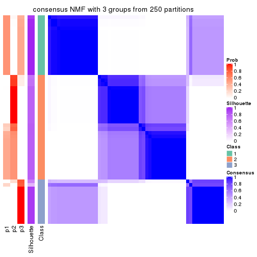
consensus_heatmap(res, k = 4)
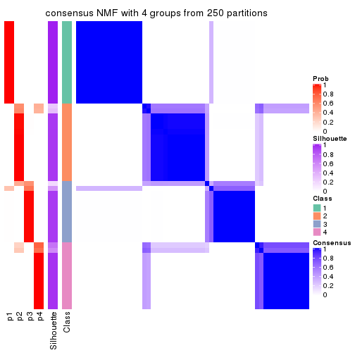
consensus_heatmap(res, k = 5)
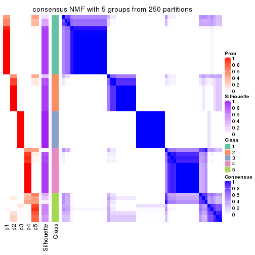
consensus_heatmap(res, k = 6)
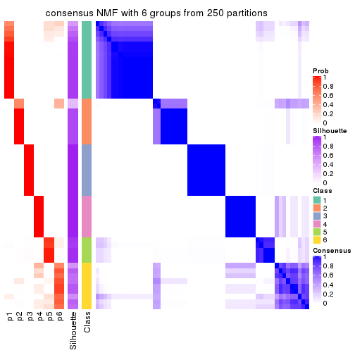
Heatmaps for the membership of samples in all partitions to see how consistent they are:
membership_heatmap(res, k = 2)

membership_heatmap(res, k = 3)
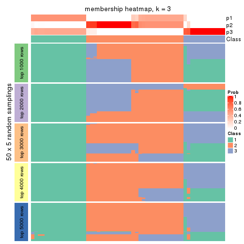
membership_heatmap(res, k = 4)
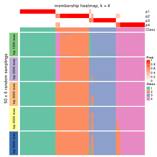
membership_heatmap(res, k = 5)
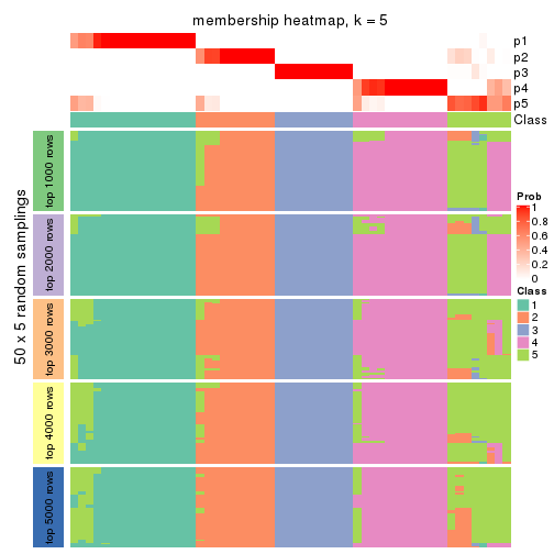
membership_heatmap(res, k = 6)
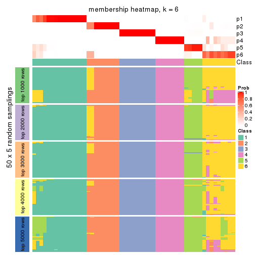
As soon as we have had the classes for columns, we can look for signatures which are significantly different between classes which can be candidate marks for certain classes. Following are the heatmaps for signatures.
Signature heatmaps where rows are scaled:
get_signatures(res, k = 2)

get_signatures(res, k = 3)
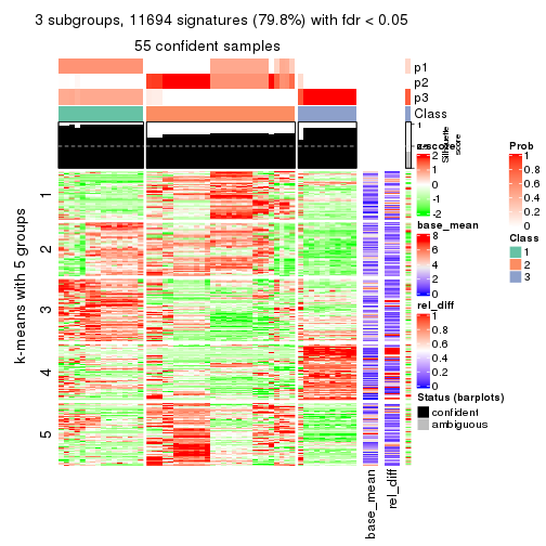
get_signatures(res, k = 4)
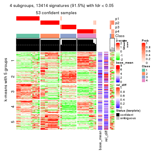
get_signatures(res, k = 5)
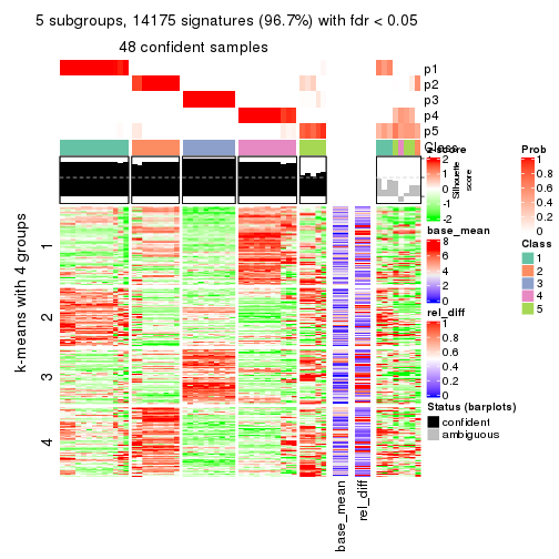
get_signatures(res, k = 6)
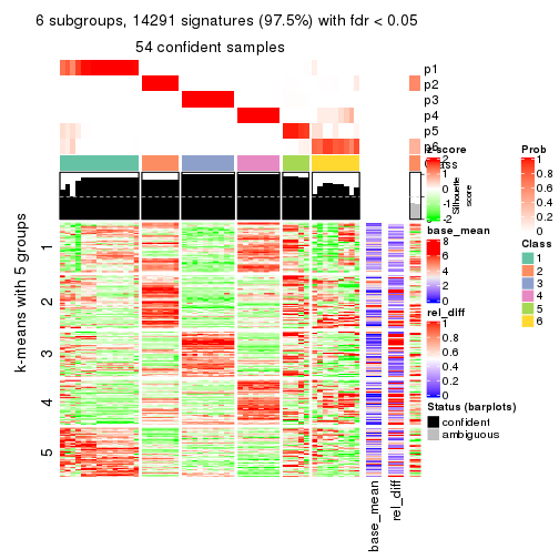
Signature heatmaps where rows are not scaled:
get_signatures(res, k = 2, scale_rows = FALSE)
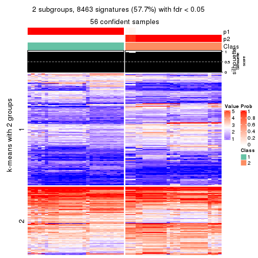
get_signatures(res, k = 3, scale_rows = FALSE)
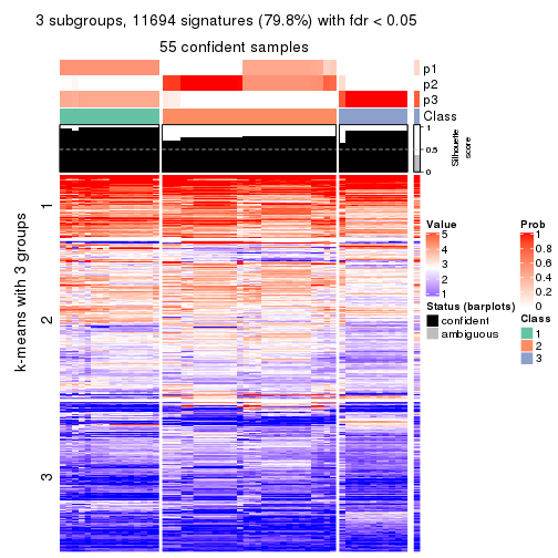
get_signatures(res, k = 4, scale_rows = FALSE)
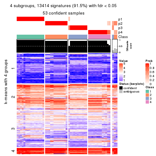
get_signatures(res, k = 5, scale_rows = FALSE)
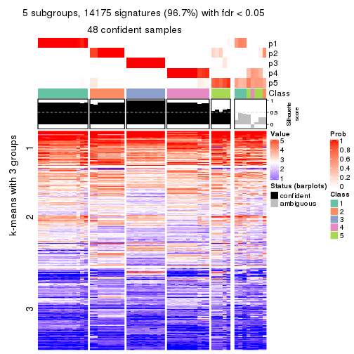
get_signatures(res, k = 6, scale_rows = FALSE)
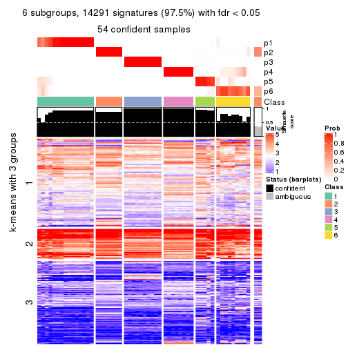
Compare the overlap of signatures from different k:
compare_signatures(res)
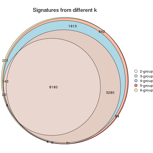
get_signature() returns a data frame invisibly. TO get the list of signatures, the function
call should be assigned to a variable explicitly. In following code, if plot argument is set
to FALSE, no heatmap is plotted while only the differential analysis is performed.
# code only for demonstration
tb = get_signature(res, k = ..., plot = FALSE)
An example of the output of tb is:
#>   which_row         fdr    mean_1    mean_2 scaled_mean_1 scaled_mean_2 km
#> 1        38 0.042760348  8.373488  9.131774    -0.5533452     0.5164555  1
#> 2        40 0.018707592  7.106213  8.469186    -0.6173731     0.5762149  1
#> 3        55 0.019134737 10.221463 11.207825    -0.6159697     0.5749050  1
#> 4        59 0.006059896  5.921854  7.869574    -0.6899429     0.6439467  1
#> 5        60 0.018055526  8.928898 10.211722    -0.6204761     0.5791110  1
#> 6        98 0.009384629 15.714769 14.887706     0.6635654    -0.6193277  2
...
The columns in tb are:
which_row: row indices corresponding to the input matrix.fdr: FDR for the differential test. mean_x: The mean value in group x.scaled_mean_x: The mean value in group x after rows are scaled.km: Row groups if k-means clustering is applied to rows.UMAP plot which shows how samples are separated.
dimension_reduction(res, k = 2, method = "UMAP")

dimension_reduction(res, k = 3, method = "UMAP")
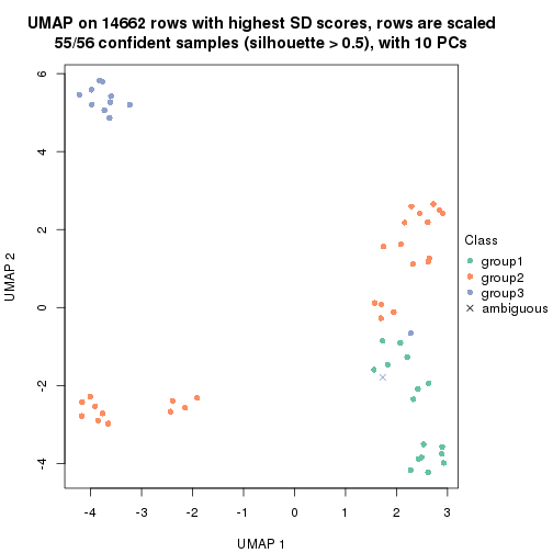
dimension_reduction(res, k = 4, method = "UMAP")
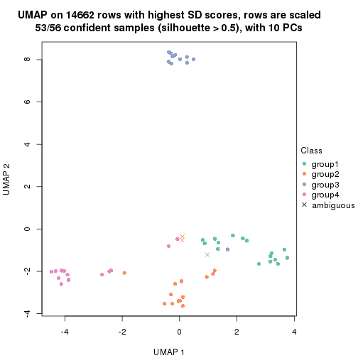
dimension_reduction(res, k = 5, method = "UMAP")
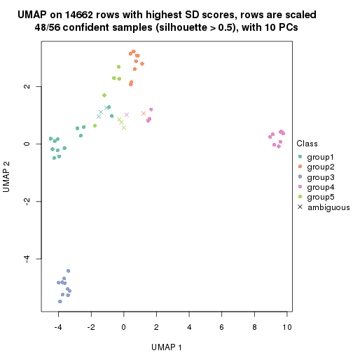
dimension_reduction(res, k = 6, method = "UMAP")
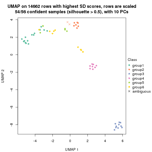
Following heatmap shows how subgroups are split when increasing k:
collect_classes(res)
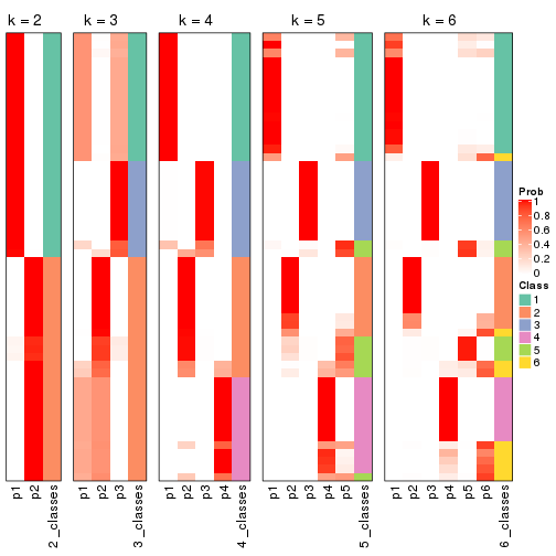
If matrix rows can be associated to genes, consider to use functional_enrichment(res,
...) to perform function enrichment for the signature genes. See this vignette for more detailed explanations.
The object with results only for a single top-value method and a single partition method can be extracted as:
res = res_list["CV", "hclust"]
# you can also extract it by
# res = res_list["CV:hclust"]
A summary of res and all the functions that can be applied to it:
res
#> A 'ConsensusPartition' object with k = 2, 3, 4, 5, 6.
#>   On a matrix with 14662 rows and 56 columns.
#>   Top rows (1000, 2000, 3000, 4000, 5000) are extracted by 'CV' method.
#>   Subgroups are detected by 'hclust' method.
#>   Performed in total 1250 partitions by row resampling.
#>   Best k for subgroups seems to be 4.
#>
#> Following methods can be applied to this 'ConsensusPartition' object:
#>  [1] "cola_report"             "collect_classes"         "collect_plots"
#>  [4] "collect_stats"           "colnames"                "compare_signatures"
#>  [7] "consensus_heatmap"       "dimension_reduction"     "functional_enrichment"
#> [10] "get_anno_col"            "get_anno"                "get_classes"
#> [13] "get_consensus"           "get_matrix"              "get_membership"
#> [16] "get_param"               "get_signatures"          "get_stats"
#> [19] "is_best_k"               "is_stable_k"             "membership_heatmap"
#> [22] "ncol"                    "nrow"                    "plot_ecdf"
#> [25] "rownames"                "select_partition_number" "show"
#> [28] "suggest_best_k"          "test_to_known_factors"
collect_plots() function collects all the plots made from res for all k (number of partitions)
into one single page to provide an easy and fast comparison between different k.
collect_plots(res)
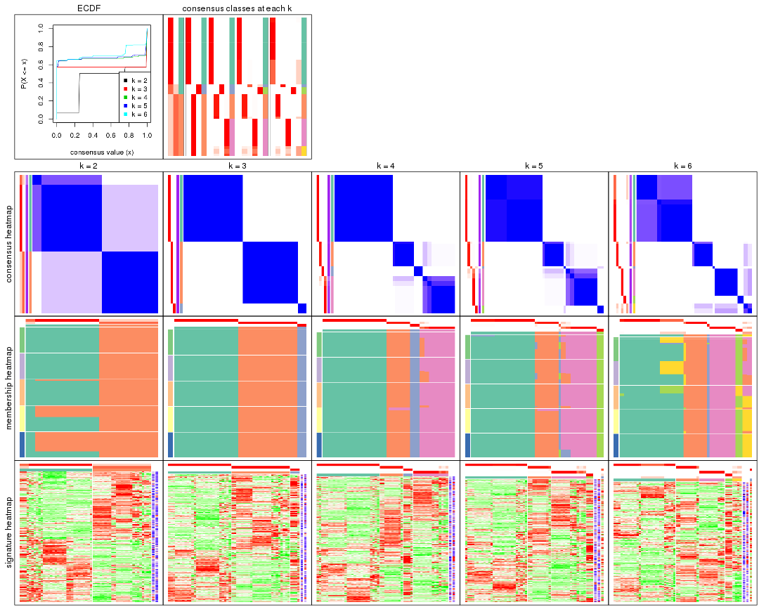
The plots are:
k and the heatmap of
predicted classes for each k.k.k.k.All the plots in panels can be made by individual functions and they are plotted later in this section.
select_partition_number() produces several plots showing different
statistics for choosing “optimized” k. There are following statistics:
k;k, the area increased is defined as \(A_k - A_{k-1}\).The detailed explanations of these statistics can be found in the cola vignette.
Generally speaking, lower PAC score, higher mean silhouette score or higher
concordance corresponds to better partition. Rand index and Jaccard index
measure how similar the current partition is compared to partition with k-1.
If they are too similar, we won't accept k is better than k-1.
select_partition_number(res)
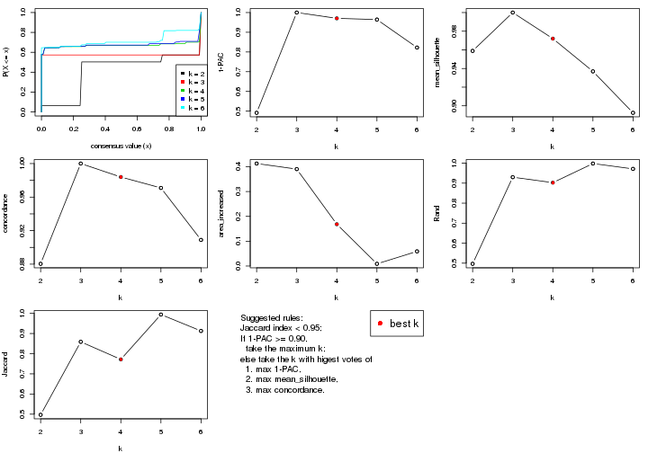
The numeric values for all these statistics can be obtained by get_stats().
get_stats(res)
#>   k 1-PAC mean_silhouette concordance area_increased  Rand Jaccard
#> 2 2 0.492           0.959       0.880        0.41271 0.497   0.497
#> 3 3 1.000           1.000       1.000        0.39032 0.930   0.859
#> 4 4 0.971           0.972       0.984        0.16836 0.903   0.772
#> 5 5 0.964           0.937       0.971        0.00888 0.998   0.994
#> 6 6 0.823           0.892       0.909        0.05903 0.971   0.913
suggest_best_k() suggests the best \(k\) based on these statistics. The rules are as follows:
suggest_best_k(res)
#> [1] 4
#> attr(,"optional")
#> [1] 3
There is also optional best \(k\) = 3 that is worth to check.
Following shows the table of the partitions (You need to click the show/hide
code output link to see it). The membership matrix (columns with name p*)
is inferred by
clue::cl_consensus()
function with the SE method. Basically the value in the membership matrix
represents the probability to belong to a certain group. The finall class
label for an item is determined with the group with highest probability it
belongs to.
In get_classes() function, the entropy is calculated from the membership
matrix and the silhouette score is calculated from the consensus matrix.
cbind(get_classes(res, k = 2), get_membership(res, k = 2))
#>           class entropy silhouette    p1    p2
#> SRR073723     1   0.000      0.956 1.000 0.000
#> SRR073724     1   0.000      0.956 1.000 0.000
#> SRR073725     1   0.000      0.956 1.000 0.000
#> SRR073726     2   0.808      1.000 0.248 0.752
#> SRR073727     1   0.000      0.956 1.000 0.000
#> SRR073728     1   0.808      0.721 0.752 0.248
#> SRR073729     1   0.808      0.721 0.752 0.248
#> SRR073730     1   0.808      0.721 0.752 0.248
#> SRR073731     2   0.808      1.000 0.248 0.752
#> SRR073732     2   0.808      1.000 0.248 0.752
#> SRR073733     2   0.808      1.000 0.248 0.752
#> SRR073734     2   0.808      1.000 0.248 0.752
#> SRR073735     2   0.808      1.000 0.248 0.752
#> SRR073736     2   0.808      1.000 0.248 0.752
#> SRR073737     2   0.808      1.000 0.248 0.752
#> SRR073738     1   0.000      0.956 1.000 0.000
#> SRR073739     1   0.000      0.956 1.000 0.000
#> SRR073740     1   0.000      0.956 1.000 0.000
#> SRR073741     1   0.000      0.956 1.000 0.000
#> SRR073742     1   0.000      0.956 1.000 0.000
#> SRR073743     1   0.000      0.956 1.000 0.000
#> SRR073744     1   0.000      0.956 1.000 0.000
#> SRR073745     1   0.000      0.956 1.000 0.000
#> SRR073746     1   0.000      0.956 1.000 0.000
#> SRR073747     1   0.000      0.956 1.000 0.000
#> SRR073748     1   0.000      0.956 1.000 0.000
#> SRR073749     1   0.000      0.956 1.000 0.000
#> SRR073750     1   0.000      0.956 1.000 0.000
#> SRR073751     1   0.808      0.721 0.752 0.248
#> SRR073752     2   0.808      1.000 0.248 0.752
#> SRR073753     2   0.808      1.000 0.248 0.752
#> SRR073754     2   0.808      1.000 0.248 0.752
#> SRR073755     2   0.808      1.000 0.248 0.752
#> SRR073756     2   0.808      1.000 0.248 0.752
#> SRR073758     2   0.808      1.000 0.248 0.752
#> SRR073759     2   0.808      1.000 0.248 0.752
#> SRR073760     2   0.808      1.000 0.248 0.752
#> SRR073761     2   0.808      1.000 0.248 0.752
#> SRR073763     2   0.808      1.000 0.248 0.752
#> SRR073764     2   0.808      1.000 0.248 0.752
#> SRR073765     2   0.808      1.000 0.248 0.752
#> SRR073766     2   0.808      1.000 0.248 0.752
#> SRR073767     2   0.808      1.000 0.248 0.752
#> SRR073768     2   0.808      1.000 0.248 0.752
#> SRR073769     1   0.000      0.956 1.000 0.000
#> SRR073770     1   0.000      0.956 1.000 0.000
#> SRR073771     1   0.000      0.956 1.000 0.000
#> SRR073772     1   0.000      0.956 1.000 0.000
#> SRR073773     1   0.000      0.956 1.000 0.000
#> SRR073774     1   0.000      0.956 1.000 0.000
#> SRR073775     1   0.000      0.956 1.000 0.000
#> SRR073776     1   0.000      0.956 1.000 0.000
#> SRR073777     1   0.000      0.956 1.000 0.000
#> SRR073778     1   0.000      0.956 1.000 0.000
#> SRR073779     2   0.808      1.000 0.248 0.752
#> SRR073780     2   0.808      1.000 0.248 0.752
cbind(get_classes(res, k = 3), get_membership(res, k = 3))
#>           class entropy silhouette p1 p2 p3
#> SRR073723     1       0          1  1  0  0
#> SRR073724     1       0          1  1  0  0
#> SRR073725     1       0          1  1  0  0
#> SRR073726     2       0          1  0  1  0
#> SRR073727     1       0          1  1  0  0
#> SRR073728     3       0          1  0  0  1
#> SRR073729     3       0          1  0  0  1
#> SRR073730     3       0          1  0  0  1
#> SRR073731     2       0          1  0  1  0
#> SRR073732     2       0          1  0  1  0
#> SRR073733     2       0          1  0  1  0
#> SRR073734     2       0          1  0  1  0
#> SRR073735     2       0          1  0  1  0
#> SRR073736     2       0          1  0  1  0
#> SRR073737     2       0          1  0  1  0
#> SRR073738     1       0          1  1  0  0
#> SRR073739     1       0          1  1  0  0
#> SRR073740     1       0          1  1  0  0
#> SRR073741     1       0          1  1  0  0
#> SRR073742     1       0          1  1  0  0
#> SRR073743     1       0          1  1  0  0
#> SRR073744     1       0          1  1  0  0
#> SRR073745     1       0          1  1  0  0
#> SRR073746     1       0          1  1  0  0
#> SRR073747     1       0          1  1  0  0
#> SRR073748     1       0          1  1  0  0
#> SRR073749     1       0          1  1  0  0
#> SRR073750     1       0          1  1  0  0
#> SRR073751     3       0          1  0  0  1
#> SRR073752     2       0          1  0  1  0
#> SRR073753     2       0          1  0  1  0
#> SRR073754     2       0          1  0  1  0
#> SRR073755     2       0          1  0  1  0
#> SRR073756     2       0          1  0  1  0
#> SRR073758     2       0          1  0  1  0
#> SRR073759     2       0          1  0  1  0
#> SRR073760     2       0          1  0  1  0
#> SRR073761     2       0          1  0  1  0
#> SRR073763     2       0          1  0  1  0
#> SRR073764     2       0          1  0  1  0
#> SRR073765     2       0          1  0  1  0
#> SRR073766     2       0          1  0  1  0
#> SRR073767     2       0          1  0  1  0
#> SRR073768     2       0          1  0  1  0
#> SRR073769     1       0          1  1  0  0
#> SRR073770     1       0          1  1  0  0
#> SRR073771     1       0          1  1  0  0
#> SRR073772     1       0          1  1  0  0
#> SRR073773     1       0          1  1  0  0
#> SRR073774     1       0          1  1  0  0
#> SRR073775     1       0          1  1  0  0
#> SRR073776     1       0          1  1  0  0
#> SRR073777     1       0          1  1  0  0
#> SRR073778     1       0          1  1  0  0
#> SRR073779     2       0          1  0  1  0
#> SRR073780     2       0          1  0  1  0
cbind(get_classes(res, k = 4), get_membership(res, k = 4))
#>           class entropy silhouette p1   p2 p3   p4
#> SRR073723     1  0.0000      1.000  1 0.00  0 0.00
#> SRR073724     1  0.0000      1.000  1 0.00  0 0.00
#> SRR073725     1  0.0000      1.000  1 0.00  0 0.00
#> SRR073726     4  0.2345      0.875  0 0.10  0 0.90
#> SRR073727     1  0.0000      1.000  1 0.00  0 0.00
#> SRR073728     3  0.0000      1.000  0 0.00  1 0.00
#> SRR073729     3  0.0000      1.000  0 0.00  1 0.00
#> SRR073730     3  0.0000      1.000  0 0.00  1 0.00
#> SRR073731     2  0.0707      0.997  0 0.98  0 0.02
#> SRR073732     2  0.0707      0.997  0 0.98  0 0.02
#> SRR073733     2  0.0707      0.997  0 0.98  0 0.02
#> SRR073734     2  0.0707      0.997  0 0.98  0 0.02
#> SRR073735     2  0.0707      0.997  0 0.98  0 0.02
#> SRR073736     2  0.0707      0.997  0 0.98  0 0.02
#> SRR073737     2  0.0707      0.997  0 0.98  0 0.02
#> SRR073738     1  0.0000      1.000  1 0.00  0 0.00
#> SRR073739     1  0.0000      1.000  1 0.00  0 0.00
#> SRR073740     1  0.0000      1.000  1 0.00  0 0.00
#> SRR073741     1  0.0000      1.000  1 0.00  0 0.00
#> SRR073742     1  0.0000      1.000  1 0.00  0 0.00
#> SRR073743     1  0.0000      1.000  1 0.00  0 0.00
#> SRR073744     1  0.0000      1.000  1 0.00  0 0.00
#> SRR073745     1  0.0000      1.000  1 0.00  0 0.00
#> SRR073746     1  0.0000      1.000  1 0.00  0 0.00
#> SRR073747     1  0.0000      1.000  1 0.00  0 0.00
#> SRR073748     1  0.0000      1.000  1 0.00  0 0.00
#> SRR073749     1  0.0000      1.000  1 0.00  0 0.00
#> SRR073750     1  0.0000      1.000  1 0.00  0 0.00
#> SRR073751     3  0.0000      1.000  0 0.00  1 0.00
#> SRR073752     2  0.0707      0.997  0 0.98  0 0.02
#> SRR073753     2  0.0707      0.997  0 0.98  0 0.02
#> SRR073754     4  0.4134      0.696  0 0.26  0 0.74
#> SRR073755     4  0.0000      0.941  0 0.00  0 1.00
#> SRR073756     4  0.0000      0.941  0 0.00  0 1.00
#> SRR073758     4  0.0000      0.941  0 0.00  0 1.00
#> SRR073759     2  0.0000      0.973  0 1.00  0 0.00
#> SRR073760     4  0.0000      0.941  0 0.00  0 1.00
#> SRR073761     4  0.0000      0.941  0 0.00  0 1.00
#> SRR073763     4  0.0000      0.941  0 0.00  0 1.00
#> SRR073764     4  0.0000      0.941  0 0.00  0 1.00
#> SRR073765     4  0.0000      0.941  0 0.00  0 1.00
#> SRR073766     4  0.0000      0.941  0 0.00  0 1.00
#> SRR073767     4  0.0000      0.941  0 0.00  0 1.00
#> SRR073768     4  0.0000      0.941  0 0.00  0 1.00
#> SRR073769     1  0.0000      1.000  1 0.00  0 0.00
#> SRR073770     1  0.0000      1.000  1 0.00  0 0.00
#> SRR073771     1  0.0000      1.000  1 0.00  0 0.00
#> SRR073772     1  0.0000      1.000  1 0.00  0 0.00
#> SRR073773     1  0.0000      1.000  1 0.00  0 0.00
#> SRR073774     1  0.0000      1.000  1 0.00  0 0.00
#> SRR073775     1  0.0000      1.000  1 0.00  0 0.00
#> SRR073776     1  0.0000      1.000  1 0.00  0 0.00
#> SRR073777     1  0.0000      1.000  1 0.00  0 0.00
#> SRR073778     1  0.0000      1.000  1 0.00  0 0.00
#> SRR073779     4  0.4134      0.696  0 0.26  0 0.74
#> SRR073780     4  0.2345      0.875  0 0.10  0 0.90
cbind(get_classes(res, k = 5), get_membership(res, k = 5))
#>           class entropy silhouette    p1    p2    p3    p4    p5
#> SRR073723     1  0.0000      0.994 1.000 0.000 0.000 0.000 0.000
#> SRR073724     1  0.0000      0.994 1.000 0.000 0.000 0.000 0.000
#> SRR073725     1  0.0000      0.994 1.000 0.000 0.000 0.000 0.000
#> SRR073726     4  0.3454      0.810 0.000 0.100 0.064 0.836 0.000
#> SRR073727     1  0.0000      0.994 1.000 0.000 0.000 0.000 0.000
#> SRR073728     5  0.0000      1.000 0.000 0.000 0.000 0.000 1.000
#> SRR073729     5  0.0000      1.000 0.000 0.000 0.000 0.000 1.000
#> SRR073730     5  0.0000      1.000 0.000 0.000 0.000 0.000 1.000
#> SRR073731     2  0.0609      0.984 0.000 0.980 0.000 0.020 0.000
#> SRR073732     2  0.0609      0.984 0.000 0.980 0.000 0.020 0.000
#> SRR073733     2  0.0609      0.984 0.000 0.980 0.000 0.020 0.000
#> SRR073734     2  0.0609      0.984 0.000 0.980 0.000 0.020 0.000
#> SRR073735     2  0.0609      0.984 0.000 0.980 0.000 0.020 0.000
#> SRR073736     2  0.0609      0.984 0.000 0.980 0.000 0.020 0.000
#> SRR073737     2  0.0609      0.984 0.000 0.980 0.000 0.020 0.000
#> SRR073738     1  0.0000      0.994 1.000 0.000 0.000 0.000 0.000
#> SRR073739     1  0.0000      0.994 1.000 0.000 0.000 0.000 0.000
#> SRR073740     1  0.0000      0.994 1.000 0.000 0.000 0.000 0.000
#> SRR073741     1  0.0000      0.994 1.000 0.000 0.000 0.000 0.000
#> SRR073742     1  0.0000      0.994 1.000 0.000 0.000 0.000 0.000
#> SRR073743     1  0.0000      0.994 1.000 0.000 0.000 0.000 0.000
#> SRR073744     1  0.0000      0.994 1.000 0.000 0.000 0.000 0.000
#> SRR073745     1  0.0000      0.994 1.000 0.000 0.000 0.000 0.000
#> SRR073746     1  0.0000      0.994 1.000 0.000 0.000 0.000 0.000
#> SRR073747     1  0.0000      0.994 1.000 0.000 0.000 0.000 0.000
#> SRR073748     1  0.0000      0.994 1.000 0.000 0.000 0.000 0.000
#> SRR073749     1  0.0000      0.994 1.000 0.000 0.000 0.000 0.000
#> SRR073750     1  0.0000      0.994 1.000 0.000 0.000 0.000 0.000
#> SRR073751     3  0.3074      0.000 0.000 0.000 0.804 0.000 0.196
#> SRR073752     2  0.0609      0.984 0.000 0.980 0.000 0.020 0.000
#> SRR073753     2  0.0609      0.984 0.000 0.980 0.000 0.020 0.000
#> SRR073754     4  0.4914      0.619 0.000 0.260 0.064 0.676 0.000
#> SRR073755     4  0.0000      0.920 0.000 0.000 0.000 1.000 0.000
#> SRR073756     4  0.0000      0.920 0.000 0.000 0.000 1.000 0.000
#> SRR073758     4  0.0000      0.920 0.000 0.000 0.000 1.000 0.000
#> SRR073759     2  0.2230      0.837 0.000 0.884 0.116 0.000 0.000
#> SRR073760     4  0.0000      0.920 0.000 0.000 0.000 1.000 0.000
#> SRR073761     4  0.0000      0.920 0.000 0.000 0.000 1.000 0.000
#> SRR073763     4  0.0000      0.920 0.000 0.000 0.000 1.000 0.000
#> SRR073764     4  0.0000      0.920 0.000 0.000 0.000 1.000 0.000
#> SRR073765     4  0.0000      0.920 0.000 0.000 0.000 1.000 0.000
#> SRR073766     4  0.0000      0.920 0.000 0.000 0.000 1.000 0.000
#> SRR073767     4  0.0000      0.920 0.000 0.000 0.000 1.000 0.000
#> SRR073768     4  0.0000      0.920 0.000 0.000 0.000 1.000 0.000
#> SRR073769     1  0.0510      0.990 0.984 0.000 0.016 0.000 0.000
#> SRR073770     1  0.0510      0.990 0.984 0.000 0.016 0.000 0.000
#> SRR073771     1  0.0510      0.990 0.984 0.000 0.016 0.000 0.000
#> SRR073772     1  0.0510      0.990 0.984 0.000 0.016 0.000 0.000
#> SRR073773     1  0.0510      0.990 0.984 0.000 0.016 0.000 0.000
#> SRR073774     1  0.0510      0.990 0.984 0.000 0.016 0.000 0.000
#> SRR073775     1  0.0510      0.990 0.984 0.000 0.016 0.000 0.000
#> SRR073776     1  0.0510      0.990 0.984 0.000 0.016 0.000 0.000
#> SRR073777     1  0.0510      0.990 0.984 0.000 0.016 0.000 0.000
#> SRR073778     1  0.0510      0.990 0.984 0.000 0.016 0.000 0.000
#> SRR073779     4  0.4914      0.619 0.000 0.260 0.064 0.676 0.000
#> SRR073780     4  0.3454      0.810 0.000 0.100 0.064 0.836 0.000
cbind(get_classes(res, k = 6), get_membership(res, k = 6))
#>           class entropy silhouette    p1   p2    p3    p4    p5    p6
#> SRR073723     1  0.0547      0.890 0.980 0.00 0.000 0.000 0.000 0.020
#> SRR073724     1  0.0547      0.890 0.980 0.00 0.000 0.000 0.000 0.020
#> SRR073725     1  0.0000      0.902 1.000 0.00 0.000 0.000 0.000 0.000
#> SRR073726     6  0.5436      0.776 0.000 0.12 0.000 0.404 0.000 0.476
#> SRR073727     1  0.0000      0.902 1.000 0.00 0.000 0.000 0.000 0.000
#> SRR073728     5  0.0000      1.000 0.000 0.00 0.000 0.000 1.000 0.000
#> SRR073729     5  0.0000      1.000 0.000 0.00 0.000 0.000 1.000 0.000
#> SRR073730     5  0.0000      1.000 0.000 0.00 0.000 0.000 1.000 0.000
#> SRR073731     2  0.0000      0.965 0.000 1.00 0.000 0.000 0.000 0.000
#> SRR073732     2  0.0000      0.965 0.000 1.00 0.000 0.000 0.000 0.000
#> SRR073733     2  0.0000      0.965 0.000 1.00 0.000 0.000 0.000 0.000
#> SRR073734     2  0.0000      0.965 0.000 1.00 0.000 0.000 0.000 0.000
#> SRR073735     2  0.0000      0.965 0.000 1.00 0.000 0.000 0.000 0.000
#> SRR073736     2  0.0000      0.965 0.000 1.00 0.000 0.000 0.000 0.000
#> SRR073737     2  0.0000      0.965 0.000 1.00 0.000 0.000 0.000 0.000
#> SRR073738     1  0.0000      0.902 1.000 0.00 0.000 0.000 0.000 0.000
#> SRR073739     1  0.0000      0.902 1.000 0.00 0.000 0.000 0.000 0.000
#> SRR073740     1  0.0000      0.902 1.000 0.00 0.000 0.000 0.000 0.000
#> SRR073741     1  0.0000      0.902 1.000 0.00 0.000 0.000 0.000 0.000
#> SRR073742     1  0.0000      0.902 1.000 0.00 0.000 0.000 0.000 0.000
#> SRR073743     1  0.0000      0.902 1.000 0.00 0.000 0.000 0.000 0.000
#> SRR073744     1  0.0000      0.902 1.000 0.00 0.000 0.000 0.000 0.000
#> SRR073745     1  0.0000      0.902 1.000 0.00 0.000 0.000 0.000 0.000
#> SRR073746     1  0.0000      0.902 1.000 0.00 0.000 0.000 0.000 0.000
#> SRR073747     1  0.0000      0.902 1.000 0.00 0.000 0.000 0.000 0.000
#> SRR073748     1  0.0000      0.902 1.000 0.00 0.000 0.000 0.000 0.000
#> SRR073749     1  0.0000      0.902 1.000 0.00 0.000 0.000 0.000 0.000
#> SRR073750     1  0.0000      0.902 1.000 0.00 0.000 0.000 0.000 0.000
#> SRR073751     3  0.0363      0.000 0.000 0.00 0.988 0.000 0.012 0.000
#> SRR073752     2  0.0000      0.965 0.000 1.00 0.000 0.000 0.000 0.000
#> SRR073753     2  0.0000      0.965 0.000 1.00 0.000 0.000 0.000 0.000
#> SRR073754     6  0.5882      0.782 0.000 0.28 0.000 0.244 0.000 0.476
#> SRR073755     4  0.0000      1.000 0.000 0.00 0.000 1.000 0.000 0.000
#> SRR073756     4  0.0000      1.000 0.000 0.00 0.000 1.000 0.000 0.000
#> SRR073758     4  0.0000      1.000 0.000 0.00 0.000 1.000 0.000 0.000
#> SRR073759     2  0.3586      0.625 0.000 0.72 0.012 0.000 0.000 0.268
#> SRR073760     4  0.0000      1.000 0.000 0.00 0.000 1.000 0.000 0.000
#> SRR073761     4  0.0000      1.000 0.000 0.00 0.000 1.000 0.000 0.000
#> SRR073763     4  0.0000      1.000 0.000 0.00 0.000 1.000 0.000 0.000
#> SRR073764     4  0.0000      1.000 0.000 0.00 0.000 1.000 0.000 0.000
#> SRR073765     4  0.0000      1.000 0.000 0.00 0.000 1.000 0.000 0.000
#> SRR073766     4  0.0000      1.000 0.000 0.00 0.000 1.000 0.000 0.000
#> SRR073767     4  0.0000      1.000 0.000 0.00 0.000 1.000 0.000 0.000
#> SRR073768     4  0.0000      1.000 0.000 0.00 0.000 1.000 0.000 0.000
#> SRR073769     1  0.3050      0.825 0.764 0.00 0.000 0.000 0.000 0.236
#> SRR073770     1  0.3050      0.825 0.764 0.00 0.000 0.000 0.000 0.236
#> SRR073771     1  0.3050      0.825 0.764 0.00 0.000 0.000 0.000 0.236
#> SRR073772     1  0.3050      0.825 0.764 0.00 0.000 0.000 0.000 0.236
#> SRR073773     1  0.3050      0.825 0.764 0.00 0.000 0.000 0.000 0.236
#> SRR073774     1  0.3050      0.825 0.764 0.00 0.000 0.000 0.000 0.236
#> SRR073775     1  0.3050      0.825 0.764 0.00 0.000 0.000 0.000 0.236
#> SRR073776     1  0.3050      0.825 0.764 0.00 0.000 0.000 0.000 0.236
#> SRR073777     1  0.3050      0.825 0.764 0.00 0.000 0.000 0.000 0.236
#> SRR073778     1  0.3050      0.825 0.764 0.00 0.000 0.000 0.000 0.236
#> SRR073779     6  0.5882      0.782 0.000 0.28 0.000 0.244 0.000 0.476
#> SRR073780     6  0.5436      0.776 0.000 0.12 0.000 0.404 0.000 0.476
Heatmaps for the consensus matrix. It visualizes the probability of two samples to be in a same group.
consensus_heatmap(res, k = 2)
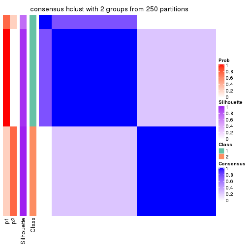
consensus_heatmap(res, k = 3)
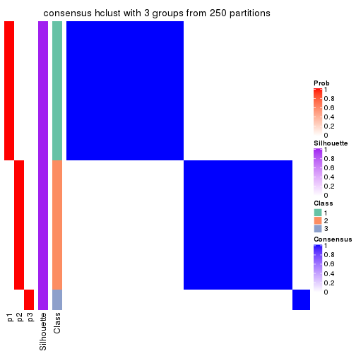
consensus_heatmap(res, k = 4)
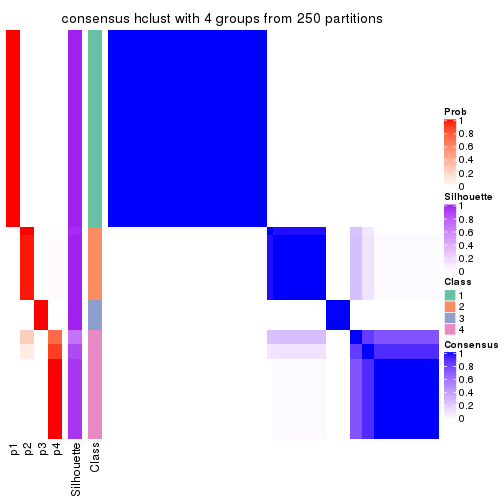
consensus_heatmap(res, k = 5)
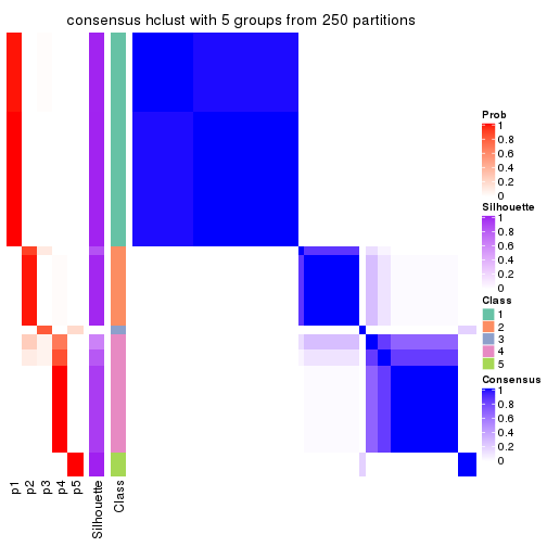
consensus_heatmap(res, k = 6)
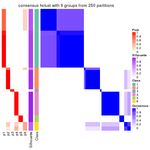
Heatmaps for the membership of samples in all partitions to see how consistent they are:
membership_heatmap(res, k = 2)
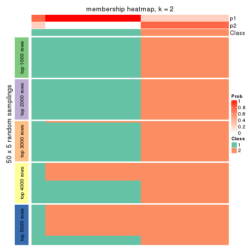
membership_heatmap(res, k = 3)
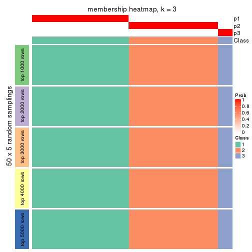
membership_heatmap(res, k = 4)
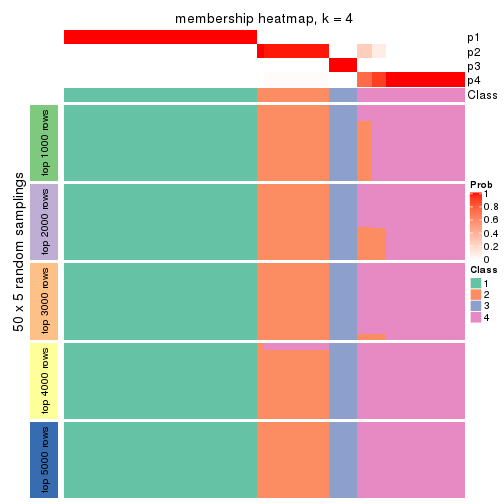
membership_heatmap(res, k = 5)
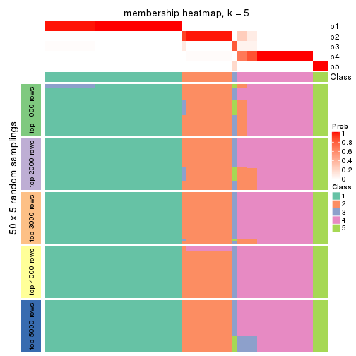
membership_heatmap(res, k = 6)
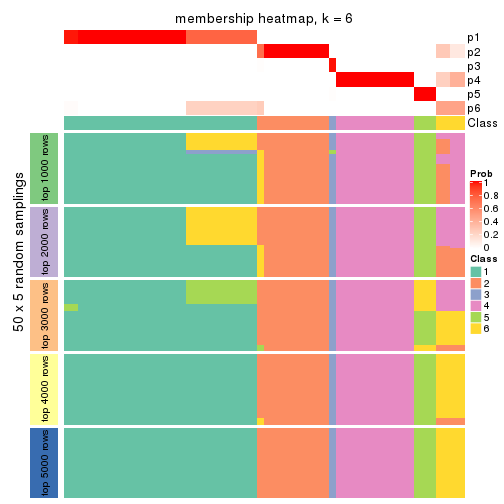
As soon as we have had the classes for columns, we can look for signatures which are significantly different between classes which can be candidate marks for certain classes. Following are the heatmaps for signatures.
Signature heatmaps where rows are scaled:
get_signatures(res, k = 2)
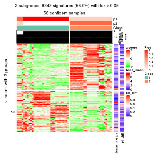
get_signatures(res, k = 3)
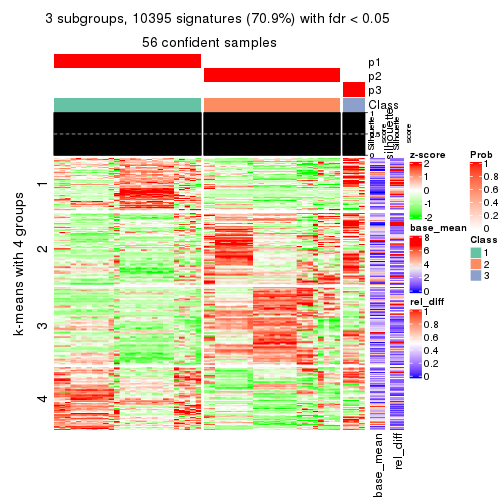
get_signatures(res, k = 4)
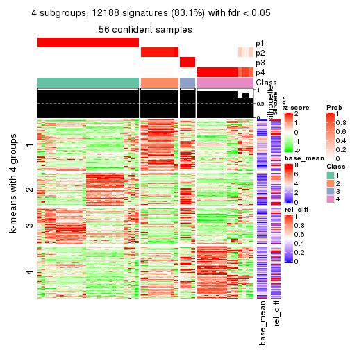
get_signatures(res, k = 5)
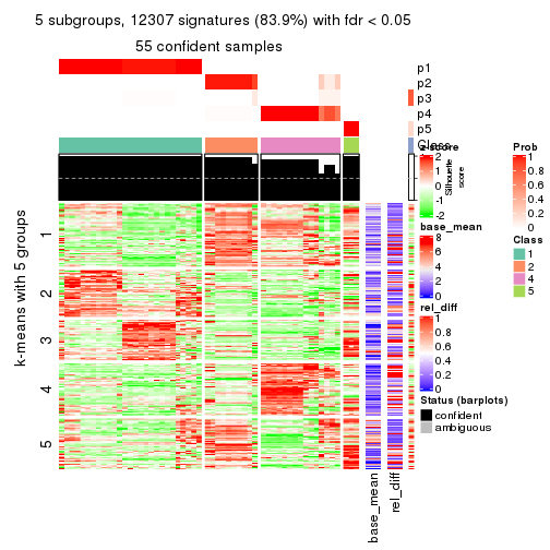
get_signatures(res, k = 6)
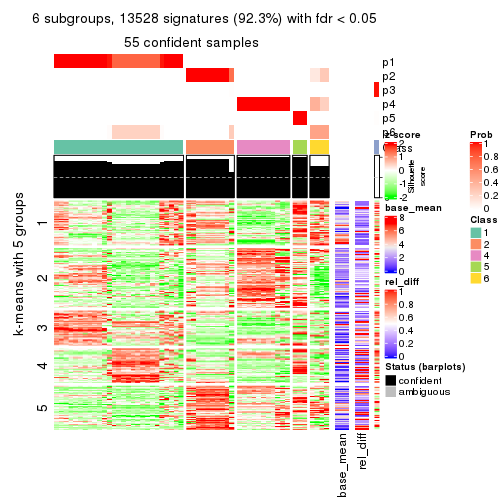
Signature heatmaps where rows are not scaled:
get_signatures(res, k = 2, scale_rows = FALSE)
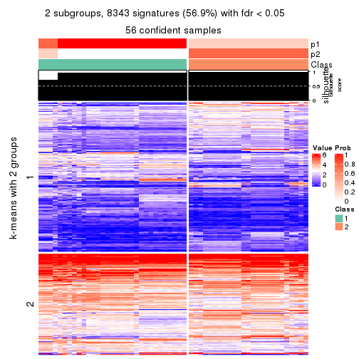
get_signatures(res, k = 3, scale_rows = FALSE)
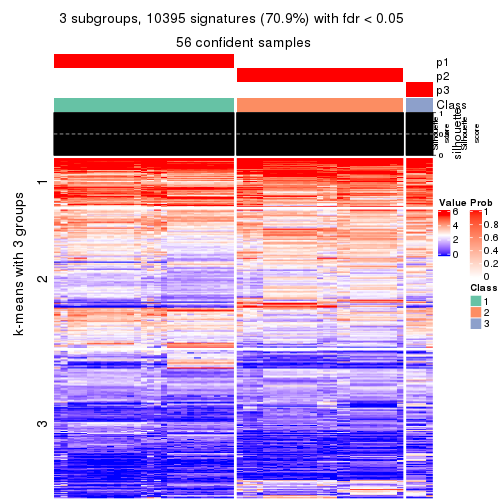
get_signatures(res, k = 4, scale_rows = FALSE)
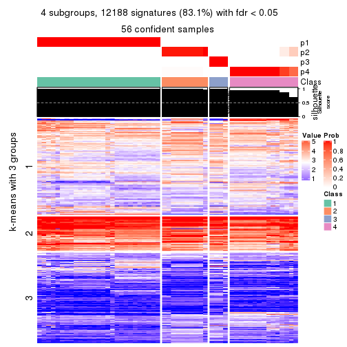
get_signatures(res, k = 5, scale_rows = FALSE)
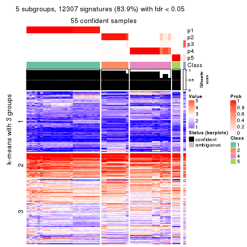
get_signatures(res, k = 6, scale_rows = FALSE)
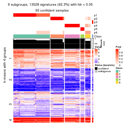
Compare the overlap of signatures from different k:
compare_signatures(res)
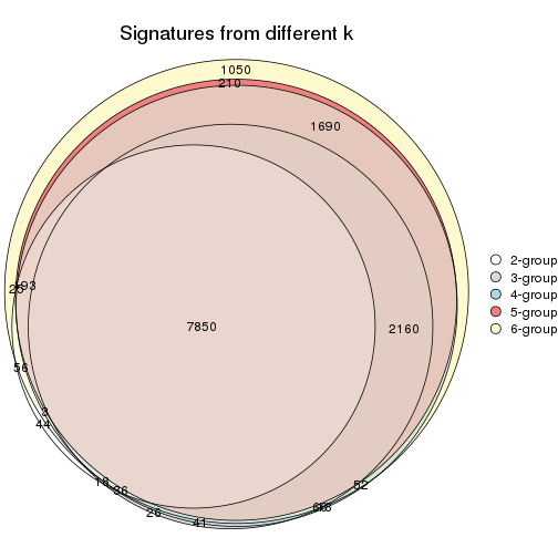
get_signature() returns a data frame invisibly. TO get the list of signatures, the function
call should be assigned to a variable explicitly. In following code, if plot argument is set
to FALSE, no heatmap is plotted while only the differential analysis is performed.
# code only for demonstration
tb = get_signature(res, k = ..., plot = FALSE)
An example of the output of tb is:
#>   which_row         fdr    mean_1    mean_2 scaled_mean_1 scaled_mean_2 km
#> 1        38 0.042760348  8.373488  9.131774    -0.5533452     0.5164555  1
#> 2        40 0.018707592  7.106213  8.469186    -0.6173731     0.5762149  1
#> 3        55 0.019134737 10.221463 11.207825    -0.6159697     0.5749050  1
#> 4        59 0.006059896  5.921854  7.869574    -0.6899429     0.6439467  1
#> 5        60 0.018055526  8.928898 10.211722    -0.6204761     0.5791110  1
#> 6        98 0.009384629 15.714769 14.887706     0.6635654    -0.6193277  2
...
The columns in tb are:
which_row: row indices corresponding to the input matrix.fdr: FDR for the differential test. mean_x: The mean value in group x.scaled_mean_x: The mean value in group x after rows are scaled.km: Row groups if k-means clustering is applied to rows.UMAP plot which shows how samples are separated.
dimension_reduction(res, k = 2, method = "UMAP")
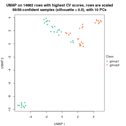
dimension_reduction(res, k = 3, method = "UMAP")

dimension_reduction(res, k = 4, method = "UMAP")
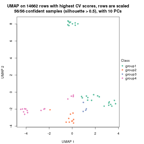
dimension_reduction(res, k = 5, method = "UMAP")
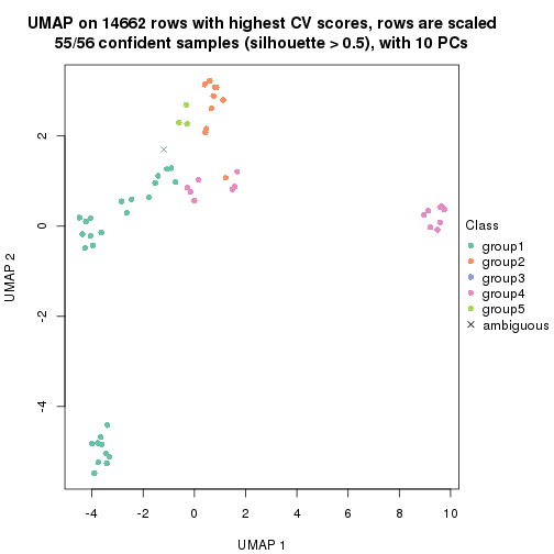
dimension_reduction(res, k = 6, method = "UMAP")
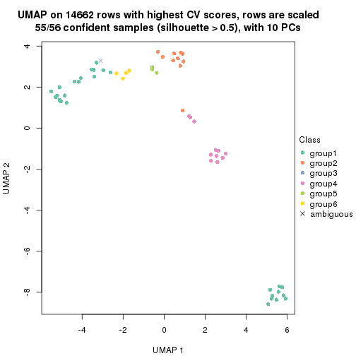
Following heatmap shows how subgroups are split when increasing k:
collect_classes(res)
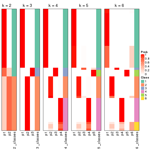
If matrix rows can be associated to genes, consider to use functional_enrichment(res,
...) to perform function enrichment for the signature genes. See this vignette for more detailed explanations.
The object with results only for a single top-value method and a single partition method can be extracted as:
res = res_list["CV", "kmeans"]
# you can also extract it by
# res = res_list["CV:kmeans"]
A summary of res and all the functions that can be applied to it:
res
#> A 'ConsensusPartition' object with k = 2, 3, 4, 5, 6.
#>   On a matrix with 14662 rows and 56 columns.
#>   Top rows (1000, 2000, 3000, 4000, 5000) are extracted by 'CV' method.
#>   Subgroups are detected by 'kmeans' method.
#>   Performed in total 1250 partitions by row resampling.
#>   Best k for subgroups seems to be 2.
#>
#> Following methods can be applied to this 'ConsensusPartition' object:
#>  [1] "cola_report"             "collect_classes"         "collect_plots"
#>  [4] "collect_stats"           "colnames"                "compare_signatures"
#>  [7] "consensus_heatmap"       "dimension_reduction"     "functional_enrichment"
#> [10] "get_anno_col"            "get_anno"                "get_classes"
#> [13] "get_consensus"           "get_matrix"              "get_membership"
#> [16] "get_param"               "get_signatures"          "get_stats"
#> [19] "is_best_k"               "is_stable_k"             "membership_heatmap"
#> [22] "ncol"                    "nrow"                    "plot_ecdf"
#> [25] "rownames"                "select_partition_number" "show"
#> [28] "suggest_best_k"          "test_to_known_factors"
collect_plots() function collects all the plots made from res for all k (number of partitions)
into one single page to provide an easy and fast comparison between different k.
collect_plots(res)
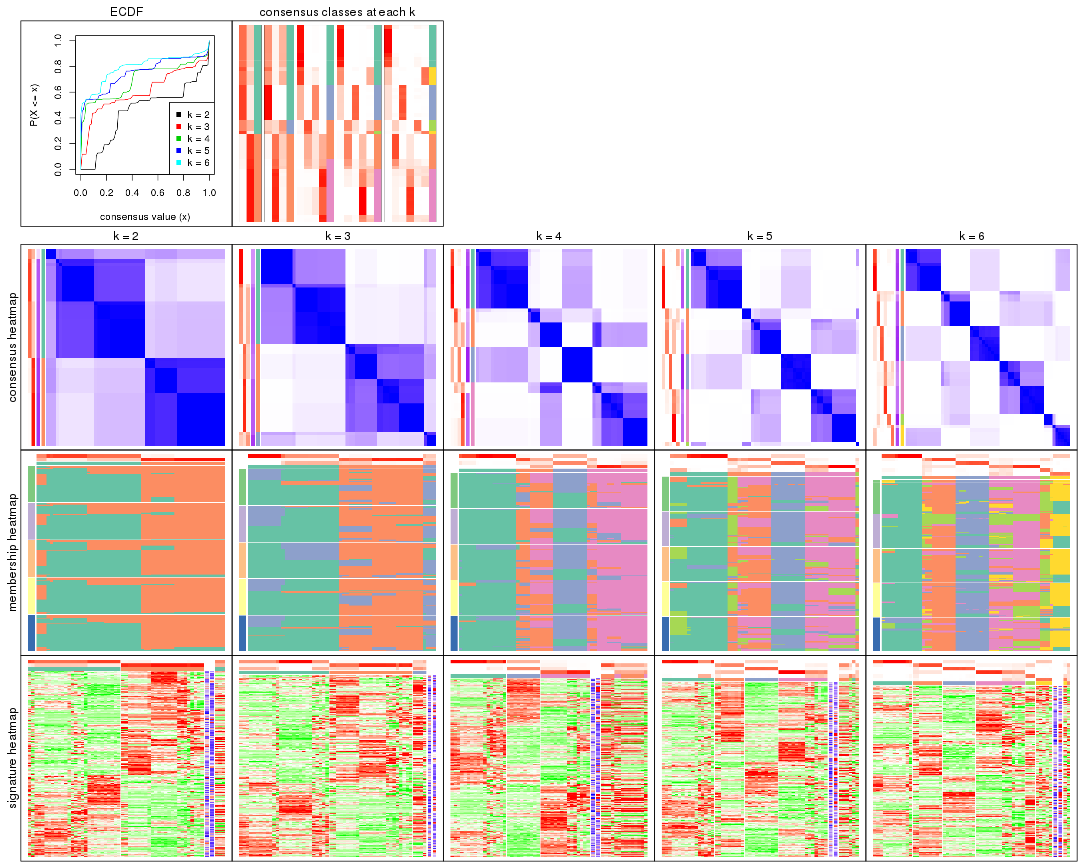
The plots are:
k and the heatmap of
predicted classes for each k.k.k.k.All the plots in panels can be made by individual functions and they are plotted later in this section.
select_partition_number() produces several plots showing different
statistics for choosing “optimized” k. There are following statistics:
k;k, the area increased is defined as \(A_k - A_{k-1}\).The detailed explanations of these statistics can be found in the cola vignette.
Generally speaking, lower PAC score, higher mean silhouette score or higher
concordance corresponds to better partition. Rand index and Jaccard index
measure how similar the current partition is compared to partition with k-1.
If they are too similar, we won't accept k is better than k-1.
select_partition_number(res)
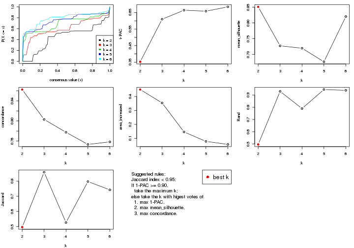
The numeric values for all these statistics can be obtained by get_stats().
get_stats(res)
#>   k 1-PAC mean_silhouette concordance area_increased  Rand Jaccard
#> 2 2 0.353           0.851       0.863         0.4498 0.497   0.497
#> 3 3 0.610           0.727       0.803         0.3538 0.930   0.859
#> 4 4 0.664           0.720       0.777         0.1461 0.790   0.527
#> 5 5 0.658           0.677       0.753         0.0784 0.945   0.797
#> 6 6 0.684           0.820       0.758         0.0565 0.938   0.743
suggest_best_k() suggests the best \(k\) based on these statistics. The rules are as follows:
suggest_best_k(res)
#> [1] 2
Following shows the table of the partitions (You need to click the show/hide
code output link to see it). The membership matrix (columns with name p*)
is inferred by
clue::cl_consensus()
function with the SE method. Basically the value in the membership matrix
represents the probability to belong to a certain group. The finall class
label for an item is determined with the group with highest probability it
belongs to.
In get_classes() function, the entropy is calculated from the membership
matrix and the silhouette score is calculated from the consensus matrix.
cbind(get_classes(res, k = 2), get_membership(res, k = 2))
#>           class entropy silhouette    p1    p2
#> SRR073723     1   0.605      0.830 0.852 0.148
#> SRR073724     1   0.844      0.843 0.728 0.272
#> SRR073725     1   0.844      0.843 0.728 0.272
#> SRR073726     2   0.118      0.961 0.016 0.984
#> SRR073727     1   0.844      0.843 0.728 0.272
#> SRR073728     1   0.961      0.198 0.616 0.384
#> SRR073729     1   0.961      0.198 0.616 0.384
#> SRR073730     1   0.961      0.198 0.616 0.384
#> SRR073731     2   0.388      0.929 0.076 0.924
#> SRR073732     2   0.388      0.929 0.076 0.924
#> SRR073733     2   0.388      0.929 0.076 0.924
#> SRR073734     2   0.388      0.929 0.076 0.924
#> SRR073735     2   0.388      0.929 0.076 0.924
#> SRR073736     2   0.388      0.929 0.076 0.924
#> SRR073737     2   0.388      0.929 0.076 0.924
#> SRR073738     1   0.844      0.843 0.728 0.272
#> SRR073739     1   0.850      0.842 0.724 0.276
#> SRR073740     1   0.850      0.842 0.724 0.276
#> SRR073741     1   0.850      0.842 0.724 0.276
#> SRR073742     1   0.850      0.842 0.724 0.276
#> SRR073743     1   0.850      0.842 0.724 0.276
#> SRR073744     1   0.850      0.842 0.724 0.276
#> SRR073745     1   0.850      0.842 0.724 0.276
#> SRR073746     1   0.850      0.842 0.724 0.276
#> SRR073747     1   0.850      0.842 0.724 0.276
#> SRR073748     1   0.850      0.842 0.724 0.276
#> SRR073749     1   0.850      0.842 0.724 0.276
#> SRR073750     1   0.833      0.843 0.736 0.264
#> SRR073751     1   0.482      0.811 0.896 0.104
#> SRR073752     2   0.295      0.930 0.052 0.948
#> SRR073753     2   0.295      0.930 0.052 0.948
#> SRR073754     2   0.118      0.961 0.016 0.984
#> SRR073755     2   0.118      0.961 0.016 0.984
#> SRR073756     2   0.118      0.961 0.016 0.984
#> SRR073758     2   0.118      0.961 0.016 0.984
#> SRR073759     2   0.278      0.933 0.048 0.952
#> SRR073760     2   0.118      0.961 0.016 0.984
#> SRR073761     2   0.118      0.961 0.016 0.984
#> SRR073763     2   0.118      0.961 0.016 0.984
#> SRR073764     2   0.118      0.961 0.016 0.984
#> SRR073765     2   0.118      0.961 0.016 0.984
#> SRR073766     2   0.118      0.961 0.016 0.984
#> SRR073767     2   0.118      0.961 0.016 0.984
#> SRR073768     2   0.118      0.961 0.016 0.984
#> SRR073769     1   0.482      0.824 0.896 0.104
#> SRR073770     1   0.482      0.824 0.896 0.104
#> SRR073771     1   0.482      0.824 0.896 0.104
#> SRR073772     1   0.482      0.824 0.896 0.104
#> SRR073773     1   0.482      0.824 0.896 0.104
#> SRR073774     1   0.482      0.824 0.896 0.104
#> SRR073775     1   0.482      0.824 0.896 0.104
#> SRR073776     1   0.482      0.824 0.896 0.104
#> SRR073777     1   0.482      0.824 0.896 0.104
#> SRR073778     1   0.482      0.824 0.896 0.104
#> SRR073779     2   0.118      0.961 0.016 0.984
#> SRR073780     2   0.118      0.961 0.016 0.984
cbind(get_classes(res, k = 3), get_membership(res, k = 3))
#>           class entropy silhouette    p1    p2    p3
#> SRR073723     1  0.6621      0.659 0.720 0.052 0.228
#> SRR073724     1  0.7890      0.760 0.544 0.060 0.396
#> SRR073725     1  0.7890      0.760 0.544 0.060 0.396
#> SRR073726     2  0.2066      0.796 0.000 0.940 0.060
#> SRR073727     1  0.7890      0.760 0.544 0.060 0.396
#> SRR073728     3  0.9187      0.937 0.272 0.196 0.532
#> SRR073729     3  0.9187      0.937 0.272 0.196 0.532
#> SRR073730     3  0.9187      0.937 0.272 0.196 0.532
#> SRR073731     2  0.6596      0.660 0.040 0.704 0.256
#> SRR073732     2  0.6596      0.660 0.040 0.704 0.256
#> SRR073733     2  0.6596      0.660 0.040 0.704 0.256
#> SRR073734     2  0.6596      0.660 0.040 0.704 0.256
#> SRR073735     2  0.6596      0.660 0.040 0.704 0.256
#> SRR073736     2  0.6596      0.660 0.040 0.704 0.256
#> SRR073737     2  0.6596      0.660 0.040 0.704 0.256
#> SRR073738     1  0.7890      0.760 0.544 0.060 0.396
#> SRR073739     1  0.7853      0.763 0.556 0.060 0.384
#> SRR073740     1  0.7853      0.763 0.556 0.060 0.384
#> SRR073741     1  0.7853      0.763 0.556 0.060 0.384
#> SRR073742     1  0.7853      0.763 0.556 0.060 0.384
#> SRR073743     1  0.7853      0.763 0.556 0.060 0.384
#> SRR073744     1  0.7853      0.763 0.556 0.060 0.384
#> SRR073745     1  0.7853      0.763 0.556 0.060 0.384
#> SRR073746     1  0.7878      0.761 0.548 0.060 0.392
#> SRR073747     1  0.7878      0.761 0.548 0.060 0.392
#> SRR073748     1  0.7878      0.761 0.548 0.060 0.392
#> SRR073749     1  0.7878      0.761 0.548 0.060 0.392
#> SRR073750     1  0.7890      0.760 0.544 0.060 0.396
#> SRR073751     3  0.9417      0.807 0.384 0.176 0.440
#> SRR073752     2  0.5158      0.716 0.004 0.764 0.232
#> SRR073753     2  0.5158      0.716 0.004 0.764 0.232
#> SRR073754     2  0.1529      0.803 0.000 0.960 0.040
#> SRR073755     2  0.1964      0.796 0.000 0.944 0.056
#> SRR073756     2  0.1964      0.796 0.000 0.944 0.056
#> SRR073758     2  0.1964      0.796 0.000 0.944 0.056
#> SRR073759     2  0.5216      0.714 0.000 0.740 0.260
#> SRR073760     2  0.1878      0.801 0.004 0.952 0.044
#> SRR073761     2  0.1878      0.801 0.004 0.952 0.044
#> SRR073763     2  0.1878      0.801 0.004 0.952 0.044
#> SRR073764     2  0.1878      0.801 0.004 0.952 0.044
#> SRR073765     2  0.1878      0.801 0.004 0.952 0.044
#> SRR073766     2  0.1878      0.801 0.004 0.952 0.044
#> SRR073767     2  0.1878      0.801 0.004 0.952 0.044
#> SRR073768     2  0.1878      0.801 0.004 0.952 0.044
#> SRR073769     1  0.0237      0.549 0.996 0.004 0.000
#> SRR073770     1  0.0237      0.549 0.996 0.004 0.000
#> SRR073771     1  0.0237      0.549 0.996 0.004 0.000
#> SRR073772     1  0.0237      0.549 0.996 0.004 0.000
#> SRR073773     1  0.0237      0.549 0.996 0.004 0.000
#> SRR073774     1  0.0237      0.549 0.996 0.004 0.000
#> SRR073775     1  0.0237      0.549 0.996 0.004 0.000
#> SRR073776     1  0.0237      0.549 0.996 0.004 0.000
#> SRR073777     1  0.0237      0.549 0.996 0.004 0.000
#> SRR073778     1  0.0237      0.549 0.996 0.004 0.000
#> SRR073779     2  0.1529      0.803 0.000 0.960 0.040
#> SRR073780     2  0.2066      0.796 0.000 0.940 0.060
cbind(get_classes(res, k = 4), get_membership(res, k = 4))
#>           class entropy silhouette    p1    p2    p3    p4
#> SRR073723     1  0.3863      0.792 0.828 0.028 0.144 0.000
#> SRR073724     1  0.2845      0.871 0.896 0.028 0.076 0.000
#> SRR073725     1  0.0469      0.933 0.988 0.000 0.012 0.000
#> SRR073726     4  0.1631      0.709 0.008 0.020 0.016 0.956
#> SRR073727     1  0.2845      0.871 0.896 0.028 0.076 0.000
#> SRR073728     2  0.3858      0.439 0.036 0.844 0.116 0.004
#> SRR073729     2  0.3858      0.439 0.036 0.844 0.116 0.004
#> SRR073730     2  0.3858      0.439 0.036 0.844 0.116 0.004
#> SRR073731     2  0.7540      0.489 0.008 0.428 0.144 0.420
#> SRR073732     2  0.7540      0.489 0.008 0.428 0.144 0.420
#> SRR073733     2  0.7540      0.489 0.008 0.428 0.144 0.420
#> SRR073734     2  0.7540      0.489 0.008 0.428 0.144 0.420
#> SRR073735     2  0.7540      0.489 0.008 0.428 0.144 0.420
#> SRR073736     2  0.7540      0.489 0.008 0.428 0.144 0.420
#> SRR073737     2  0.7540      0.489 0.008 0.428 0.144 0.420
#> SRR073738     1  0.2845      0.871 0.896 0.028 0.076 0.000
#> SRR073739     1  0.0336      0.938 0.992 0.000 0.008 0.000
#> SRR073740     1  0.0336      0.938 0.992 0.000 0.008 0.000
#> SRR073741     1  0.0336      0.938 0.992 0.000 0.008 0.000
#> SRR073742     1  0.0336      0.938 0.992 0.000 0.008 0.000
#> SRR073743     1  0.0336      0.938 0.992 0.000 0.008 0.000
#> SRR073744     1  0.0336      0.938 0.992 0.000 0.008 0.000
#> SRR073745     1  0.0336      0.938 0.992 0.000 0.008 0.000
#> SRR073746     1  0.0000      0.939 1.000 0.000 0.000 0.000
#> SRR073747     1  0.0000      0.939 1.000 0.000 0.000 0.000
#> SRR073748     1  0.0000      0.939 1.000 0.000 0.000 0.000
#> SRR073749     1  0.0000      0.939 1.000 0.000 0.000 0.000
#> SRR073750     1  0.2845      0.871 0.896 0.028 0.076 0.000
#> SRR073751     2  0.4731      0.386 0.060 0.780 0.160 0.000
#> SRR073752     4  0.7489     -0.442 0.004 0.388 0.156 0.452
#> SRR073753     4  0.7489     -0.442 0.004 0.388 0.156 0.452
#> SRR073754     4  0.1271      0.713 0.008 0.012 0.012 0.968
#> SRR073755     4  0.0992      0.717 0.008 0.012 0.004 0.976
#> SRR073756     4  0.0992      0.717 0.008 0.012 0.004 0.976
#> SRR073758     4  0.0992      0.717 0.008 0.012 0.004 0.976
#> SRR073759     4  0.7258     -0.342 0.000 0.328 0.164 0.508
#> SRR073760     4  0.5229      0.735 0.032 0.048 0.140 0.780
#> SRR073761     4  0.5229      0.735 0.032 0.048 0.140 0.780
#> SRR073763     4  0.5229      0.735 0.032 0.048 0.140 0.780
#> SRR073764     4  0.5229      0.735 0.032 0.048 0.140 0.780
#> SRR073765     4  0.5229      0.735 0.032 0.048 0.140 0.780
#> SRR073766     4  0.5229      0.735 0.032 0.048 0.140 0.780
#> SRR073767     4  0.5229      0.735 0.032 0.048 0.140 0.780
#> SRR073768     4  0.5229      0.735 0.032 0.048 0.140 0.780
#> SRR073769     3  0.4830      1.000 0.392 0.000 0.608 0.000
#> SRR073770     3  0.4830      1.000 0.392 0.000 0.608 0.000
#> SRR073771     3  0.4830      1.000 0.392 0.000 0.608 0.000
#> SRR073772     3  0.4830      1.000 0.392 0.000 0.608 0.000
#> SRR073773     3  0.4830      1.000 0.392 0.000 0.608 0.000
#> SRR073774     3  0.4830      1.000 0.392 0.000 0.608 0.000
#> SRR073775     3  0.4830      1.000 0.392 0.000 0.608 0.000
#> SRR073776     3  0.4830      1.000 0.392 0.000 0.608 0.000
#> SRR073777     3  0.4830      1.000 0.392 0.000 0.608 0.000
#> SRR073778     3  0.4830      1.000 0.392 0.000 0.608 0.000
#> SRR073779     4  0.1271      0.713 0.008 0.012 0.012 0.968
#> SRR073780     4  0.1631      0.709 0.008 0.020 0.016 0.956
cbind(get_classes(res, k = 5), get_membership(res, k = 5))
#>           class entropy silhouette    p1    p2    p3    p4    p5
#> SRR073723     1  0.4848      0.466 0.556 0.000 0.024 0.000 0.420
#> SRR073724     1  0.4227      0.506 0.580 0.000 0.000 0.000 0.420
#> SRR073725     1  0.1043      0.831 0.960 0.000 0.000 0.000 0.040
#> SRR073726     4  0.5989      0.660 0.000 0.084 0.020 0.584 0.312
#> SRR073727     1  0.4227      0.506 0.580 0.000 0.000 0.000 0.420
#> SRR073728     2  0.6269     -0.445 0.004 0.592 0.172 0.008 0.224
#> SRR073729     2  0.6269     -0.445 0.004 0.592 0.172 0.008 0.224
#> SRR073730     2  0.6269     -0.445 0.004 0.592 0.172 0.008 0.224
#> SRR073731     2  0.4706      0.659 0.020 0.632 0.004 0.344 0.000
#> SRR073732     2  0.4706      0.659 0.020 0.632 0.004 0.344 0.000
#> SRR073733     2  0.4706      0.659 0.020 0.632 0.004 0.344 0.000
#> SRR073734     2  0.4706      0.659 0.020 0.632 0.004 0.344 0.000
#> SRR073735     2  0.4706      0.659 0.020 0.632 0.004 0.344 0.000
#> SRR073736     2  0.4706      0.659 0.020 0.632 0.004 0.344 0.000
#> SRR073737     2  0.4706      0.659 0.020 0.632 0.004 0.344 0.000
#> SRR073738     1  0.4227      0.506 0.580 0.000 0.000 0.000 0.420
#> SRR073739     1  0.0162      0.845 0.996 0.000 0.000 0.004 0.000
#> SRR073740     1  0.0162      0.845 0.996 0.000 0.000 0.004 0.000
#> SRR073741     1  0.0162      0.845 0.996 0.000 0.000 0.004 0.000
#> SRR073742     1  0.0162      0.845 0.996 0.000 0.000 0.004 0.000
#> SRR073743     1  0.0162      0.845 0.996 0.000 0.000 0.004 0.000
#> SRR073744     1  0.0162      0.845 0.996 0.000 0.000 0.004 0.000
#> SRR073745     1  0.0162      0.845 0.996 0.000 0.000 0.004 0.000
#> SRR073746     1  0.0162      0.845 0.996 0.000 0.000 0.004 0.000
#> SRR073747     1  0.0671      0.843 0.980 0.000 0.000 0.004 0.016
#> SRR073748     1  0.0671      0.843 0.980 0.000 0.000 0.004 0.016
#> SRR073749     1  0.0671      0.843 0.980 0.000 0.000 0.004 0.016
#> SRR073750     1  0.4227      0.506 0.580 0.000 0.000 0.000 0.420
#> SRR073751     5  0.6146      0.000 0.020 0.240 0.116 0.004 0.620
#> SRR073752     2  0.6852      0.517 0.000 0.528 0.052 0.304 0.116
#> SRR073753     2  0.6852      0.517 0.000 0.528 0.052 0.304 0.116
#> SRR073754     4  0.5870      0.669 0.000 0.084 0.024 0.624 0.268
#> SRR073755     4  0.5801      0.687 0.000 0.068 0.028 0.624 0.280
#> SRR073756     4  0.5801      0.687 0.000 0.068 0.028 0.624 0.280
#> SRR073758     4  0.5801      0.687 0.000 0.068 0.028 0.624 0.280
#> SRR073759     2  0.7706      0.291 0.000 0.404 0.060 0.280 0.256
#> SRR073760     4  0.0000      0.752 0.000 0.000 0.000 1.000 0.000
#> SRR073761     4  0.0000      0.752 0.000 0.000 0.000 1.000 0.000
#> SRR073763     4  0.0000      0.752 0.000 0.000 0.000 1.000 0.000
#> SRR073764     4  0.0000      0.752 0.000 0.000 0.000 1.000 0.000
#> SRR073765     4  0.0000      0.752 0.000 0.000 0.000 1.000 0.000
#> SRR073766     4  0.0000      0.752 0.000 0.000 0.000 1.000 0.000
#> SRR073767     4  0.0000      0.752 0.000 0.000 0.000 1.000 0.000
#> SRR073768     4  0.0000      0.752 0.000 0.000 0.000 1.000 0.000
#> SRR073769     3  0.3582      0.994 0.224 0.000 0.768 0.000 0.008
#> SRR073770     3  0.3720      0.993 0.228 0.000 0.760 0.000 0.012
#> SRR073771     3  0.3305      0.994 0.224 0.000 0.776 0.000 0.000
#> SRR073772     3  0.3612      0.993 0.228 0.000 0.764 0.000 0.008
#> SRR073773     3  0.3491      0.993 0.228 0.000 0.768 0.000 0.004
#> SRR073774     3  0.3461      0.994 0.224 0.000 0.772 0.000 0.004
#> SRR073775     3  0.3305      0.994 0.224 0.000 0.776 0.000 0.000
#> SRR073776     3  0.3461      0.994 0.224 0.000 0.772 0.000 0.004
#> SRR073777     3  0.3612      0.993 0.228 0.000 0.764 0.000 0.008
#> SRR073778     3  0.3461      0.994 0.224 0.000 0.772 0.000 0.004
#> SRR073779     4  0.5870      0.669 0.000 0.084 0.024 0.624 0.268
#> SRR073780     4  0.5989      0.660 0.000 0.084 0.020 0.584 0.312
cbind(get_classes(res, k = 6), get_membership(res, k = 6))
#>           class entropy silhouette    p1    p2    p3    p4    p5    p6
#> SRR073723     6  0.3738      0.878 0.280 0.000 0.016 0.000 0.000 0.704
#> SRR073724     6  0.3390      0.888 0.296 0.000 0.000 0.000 0.000 0.704
#> SRR073725     1  0.2918      0.887 0.868 0.064 0.000 0.000 0.048 0.020
#> SRR073726     4  0.7298      0.574 0.000 0.088 0.072 0.536 0.132 0.172
#> SRR073727     6  0.3528      0.889 0.296 0.004 0.000 0.000 0.000 0.700
#> SRR073728     5  0.4049      1.000 0.004 0.256 0.032 0.000 0.708 0.000
#> SRR073729     5  0.4049      1.000 0.004 0.256 0.032 0.000 0.708 0.000
#> SRR073730     5  0.4049      1.000 0.004 0.256 0.032 0.000 0.708 0.000
#> SRR073731     2  0.2402      0.839 0.000 0.856 0.004 0.140 0.000 0.000
#> SRR073732     2  0.2402      0.839 0.000 0.856 0.004 0.140 0.000 0.000
#> SRR073733     2  0.2402      0.839 0.000 0.856 0.004 0.140 0.000 0.000
#> SRR073734     2  0.2402      0.839 0.000 0.856 0.004 0.140 0.000 0.000
#> SRR073735     2  0.2402      0.839 0.000 0.856 0.004 0.140 0.000 0.000
#> SRR073736     2  0.2402      0.839 0.000 0.856 0.004 0.140 0.000 0.000
#> SRR073737     2  0.2402      0.839 0.000 0.856 0.004 0.140 0.000 0.000
#> SRR073738     6  0.3973      0.882 0.296 0.012 0.000 0.000 0.008 0.684
#> SRR073739     1  0.0000      0.944 1.000 0.000 0.000 0.000 0.000 0.000
#> SRR073740     1  0.0000      0.944 1.000 0.000 0.000 0.000 0.000 0.000
#> SRR073741     1  0.0000      0.944 1.000 0.000 0.000 0.000 0.000 0.000
#> SRR073742     1  0.0000      0.944 1.000 0.000 0.000 0.000 0.000 0.000
#> SRR073743     1  0.0000      0.944 1.000 0.000 0.000 0.000 0.000 0.000
#> SRR073744     1  0.0000      0.944 1.000 0.000 0.000 0.000 0.000 0.000
#> SRR073745     1  0.0000      0.944 1.000 0.000 0.000 0.000 0.000 0.000
#> SRR073746     1  0.0993      0.934 0.964 0.024 0.000 0.000 0.012 0.000
#> SRR073747     1  0.2739      0.895 0.876 0.064 0.000 0.000 0.048 0.012
#> SRR073748     1  0.2739      0.895 0.876 0.064 0.000 0.000 0.048 0.012
#> SRR073749     1  0.2739      0.895 0.876 0.064 0.000 0.000 0.048 0.012
#> SRR073750     6  0.3772      0.887 0.296 0.008 0.000 0.000 0.004 0.692
#> SRR073751     6  0.5499      0.355 0.020 0.104 0.016 0.000 0.208 0.652
#> SRR073752     2  0.6921      0.633 0.000 0.572 0.120 0.160 0.104 0.044
#> SRR073753     2  0.6921      0.633 0.000 0.572 0.120 0.160 0.104 0.044
#> SRR073754     4  0.7379      0.569 0.000 0.096 0.076 0.532 0.148 0.148
#> SRR073755     4  0.6493      0.608 0.000 0.064 0.040 0.580 0.080 0.236
#> SRR073756     4  0.6493      0.608 0.000 0.064 0.040 0.580 0.080 0.236
#> SRR073758     4  0.6493      0.608 0.000 0.064 0.040 0.580 0.080 0.236
#> SRR073759     2  0.8547      0.379 0.000 0.368 0.140 0.180 0.152 0.160
#> SRR073760     4  0.1267      0.709 0.000 0.060 0.000 0.940 0.000 0.000
#> SRR073761     4  0.1555      0.709 0.000 0.060 0.004 0.932 0.004 0.000
#> SRR073763     4  0.1411      0.709 0.000 0.060 0.004 0.936 0.000 0.000
#> SRR073764     4  0.1555      0.709 0.000 0.060 0.004 0.932 0.004 0.000
#> SRR073765     4  0.1267      0.709 0.000 0.060 0.000 0.940 0.000 0.000
#> SRR073766     4  0.1411      0.709 0.000 0.060 0.000 0.936 0.004 0.000
#> SRR073767     4  0.1555      0.709 0.000 0.060 0.004 0.932 0.004 0.000
#> SRR073768     4  0.1267      0.709 0.000 0.060 0.000 0.940 0.000 0.000
#> SRR073769     3  0.2416      0.979 0.156 0.000 0.844 0.000 0.000 0.000
#> SRR073770     3  0.3800      0.965 0.156 0.024 0.792 0.000 0.020 0.008
#> SRR073771     3  0.3252      0.976 0.156 0.008 0.816 0.000 0.004 0.016
#> SRR073772     3  0.4054      0.960 0.156 0.024 0.780 0.000 0.028 0.012
#> SRR073773     3  0.2952      0.978 0.156 0.008 0.828 0.000 0.004 0.004
#> SRR073774     3  0.2700      0.978 0.156 0.004 0.836 0.000 0.000 0.004
#> SRR073775     3  0.2810      0.978 0.156 0.004 0.832 0.000 0.000 0.008
#> SRR073776     3  0.2700      0.977 0.156 0.004 0.836 0.000 0.000 0.004
#> SRR073777     3  0.4054      0.960 0.156 0.024 0.780 0.000 0.028 0.012
#> SRR073778     3  0.2700      0.977 0.156 0.004 0.836 0.000 0.000 0.004
#> SRR073779     4  0.7379      0.569 0.000 0.096 0.076 0.532 0.148 0.148
#> SRR073780     4  0.7298      0.574 0.000 0.088 0.072 0.536 0.132 0.172
Heatmaps for the consensus matrix. It visualizes the probability of two samples to be in a same group.
consensus_heatmap(res, k = 2)
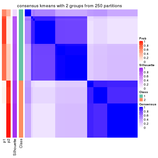
consensus_heatmap(res, k = 3)
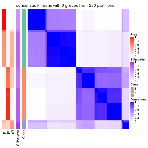
consensus_heatmap(res, k = 4)
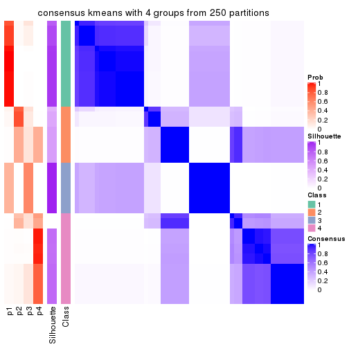
consensus_heatmap(res, k = 5)
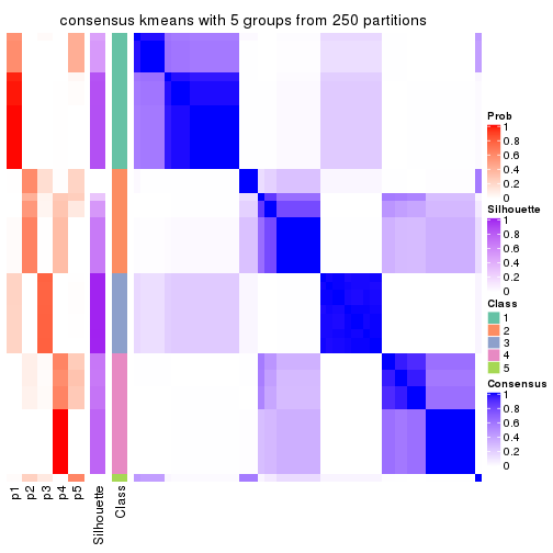
consensus_heatmap(res, k = 6)
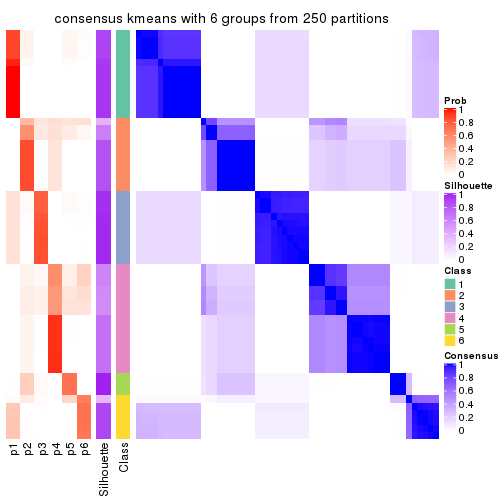
Heatmaps for the membership of samples in all partitions to see how consistent they are:
membership_heatmap(res, k = 2)
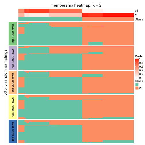
membership_heatmap(res, k = 3)
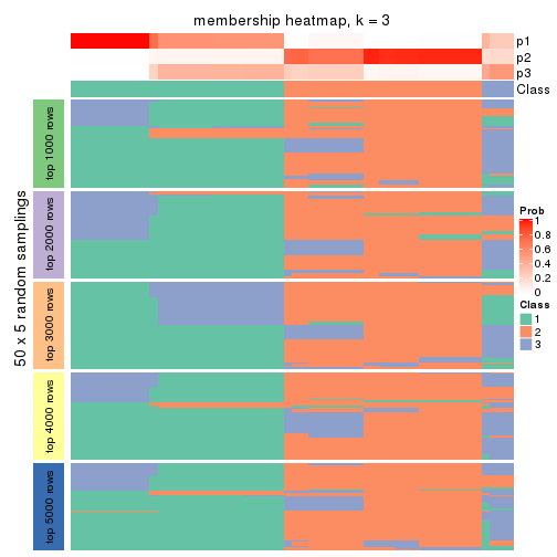
membership_heatmap(res, k = 4)
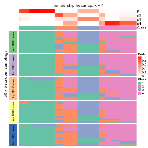
membership_heatmap(res, k = 5)
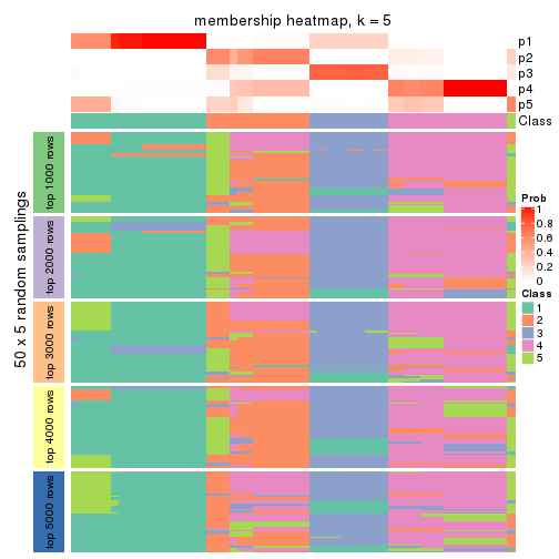
membership_heatmap(res, k = 6)
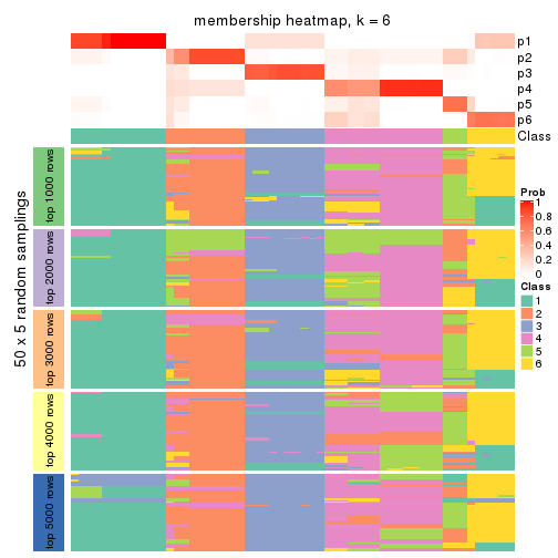
As soon as we have had the classes for columns, we can look for signatures which are significantly different between classes which can be candidate marks for certain classes. Following are the heatmaps for signatures.
Signature heatmaps where rows are scaled:
get_signatures(res, k = 2)
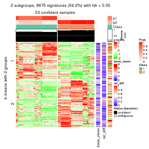
get_signatures(res, k = 3)
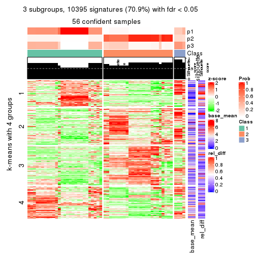
get_signatures(res, k = 4)
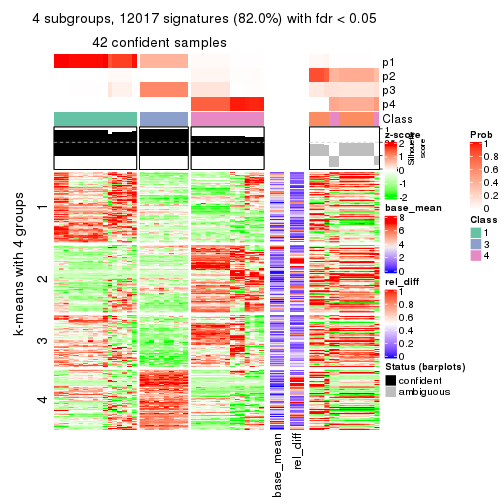
get_signatures(res, k = 5)
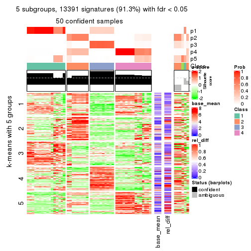
get_signatures(res, k = 6)
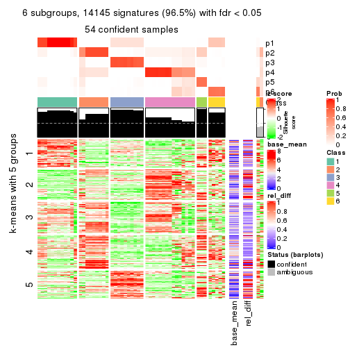
Signature heatmaps where rows are not scaled:
get_signatures(res, k = 2, scale_rows = FALSE)
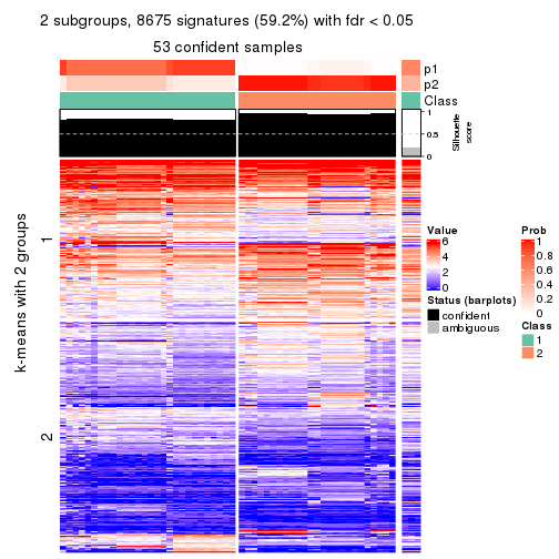
get_signatures(res, k = 3, scale_rows = FALSE)
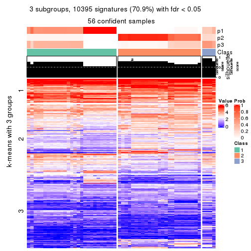
get_signatures(res, k = 4, scale_rows = FALSE)
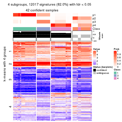
get_signatures(res, k = 5, scale_rows = FALSE)
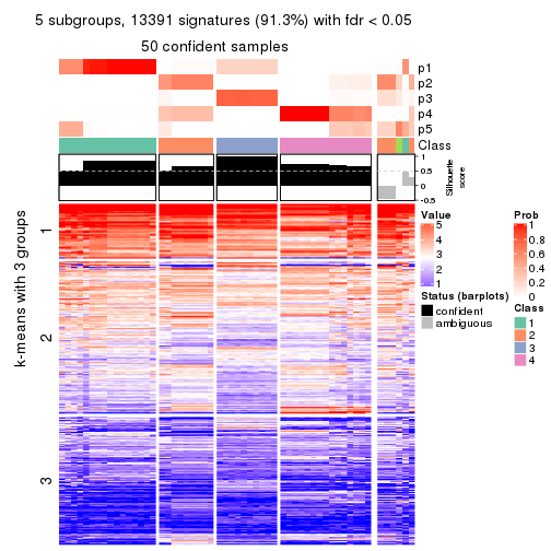
get_signatures(res, k = 6, scale_rows = FALSE)
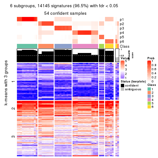
Compare the overlap of signatures from different k:
compare_signatures(res)
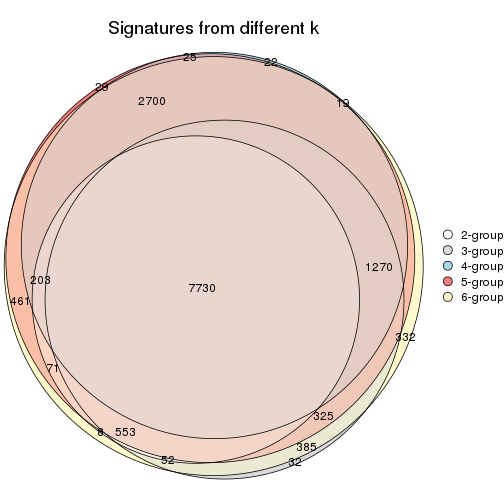
get_signature() returns a data frame invisibly. TO get the list of signatures, the function
call should be assigned to a variable explicitly. In following code, if plot argument is set
to FALSE, no heatmap is plotted while only the differential analysis is performed.
# code only for demonstration
tb = get_signature(res, k = ..., plot = FALSE)
An example of the output of tb is:
#>   which_row         fdr    mean_1    mean_2 scaled_mean_1 scaled_mean_2 km
#> 1        38 0.042760348  8.373488  9.131774    -0.5533452     0.5164555  1
#> 2        40 0.018707592  7.106213  8.469186    -0.6173731     0.5762149  1
#> 3        55 0.019134737 10.221463 11.207825    -0.6159697     0.5749050  1
#> 4        59 0.006059896  5.921854  7.869574    -0.6899429     0.6439467  1
#> 5        60 0.018055526  8.928898 10.211722    -0.6204761     0.5791110  1
#> 6        98 0.009384629 15.714769 14.887706     0.6635654    -0.6193277  2
...
The columns in tb are:
which_row: row indices corresponding to the input matrix.fdr: FDR for the differential test. mean_x: The mean value in group x.scaled_mean_x: The mean value in group x after rows are scaled.km: Row groups if k-means clustering is applied to rows.UMAP plot which shows how samples are separated.
dimension_reduction(res, k = 2, method = "UMAP")

dimension_reduction(res, k = 3, method = "UMAP")
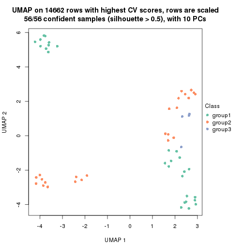
dimension_reduction(res, k = 4, method = "UMAP")
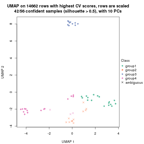
dimension_reduction(res, k = 5, method = "UMAP")

dimension_reduction(res, k = 6, method = "UMAP")
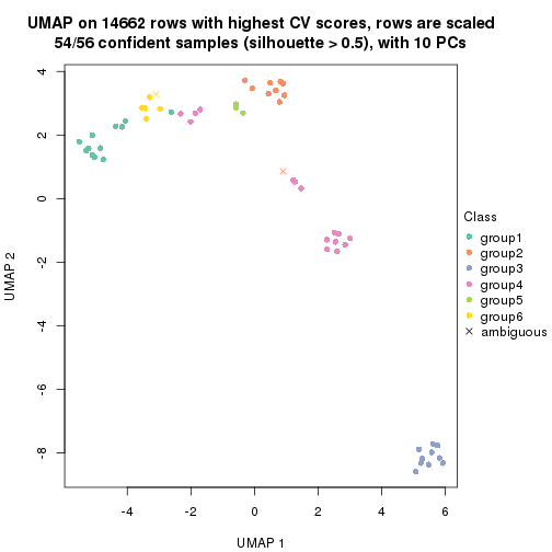
Following heatmap shows how subgroups are split when increasing k:
collect_classes(res)
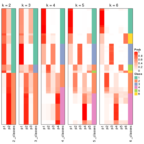
If matrix rows can be associated to genes, consider to use functional_enrichment(res,
...) to perform function enrichment for the signature genes. See this vignette for more detailed explanations.
The object with results only for a single top-value method and a single partition method can be extracted as:
res = res_list["CV", "skmeans"]
# you can also extract it by
# res = res_list["CV:skmeans"]
A summary of res and all the functions that can be applied to it:
res
#> A 'ConsensusPartition' object with k = 2, 3, 4, 5, 6.
#>   On a matrix with 14662 rows and 56 columns.
#>   Top rows (1000, 2000, 3000, 4000, 5000) are extracted by 'CV' method.
#>   Subgroups are detected by 'skmeans' method.
#>   Performed in total 1250 partitions by row resampling.
#>   Best k for subgroups seems to be 6.
#>
#> Following methods can be applied to this 'ConsensusPartition' object:
#>  [1] "cola_report"             "collect_classes"         "collect_plots"
#>  [4] "collect_stats"           "colnames"                "compare_signatures"
#>  [7] "consensus_heatmap"       "dimension_reduction"     "functional_enrichment"
#> [10] "get_anno_col"            "get_anno"                "get_classes"
#> [13] "get_consensus"           "get_matrix"              "get_membership"
#> [16] "get_param"               "get_signatures"          "get_stats"
#> [19] "is_best_k"               "is_stable_k"             "membership_heatmap"
#> [22] "ncol"                    "nrow"                    "plot_ecdf"
#> [25] "rownames"                "select_partition_number" "show"
#> [28] "suggest_best_k"          "test_to_known_factors"
collect_plots() function collects all the plots made from res for all k (number of partitions)
into one single page to provide an easy and fast comparison between different k.
collect_plots(res)
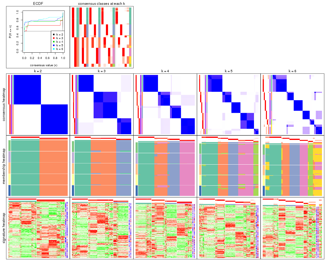
The plots are:
k and the heatmap of
predicted classes for each k.k.k.k.All the plots in panels can be made by individual functions and they are plotted later in this section.
select_partition_number() produces several plots showing different
statistics for choosing “optimized” k. There are following statistics:
k;k, the area increased is defined as \(A_k - A_{k-1}\).The detailed explanations of these statistics can be found in the cola vignette.
Generally speaking, lower PAC score, higher mean silhouette score or higher
concordance corresponds to better partition. Rand index and Jaccard index
measure how similar the current partition is compared to partition with k-1.
If they are too similar, we won't accept k is better than k-1.
select_partition_number(res)
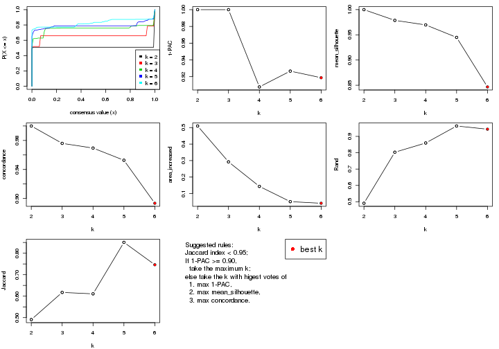
The numeric values for all these statistics can be obtained by get_stats().
get_stats(res)
#>   k 1-PAC mean_silhouette concordance area_increased  Rand Jaccard
#> 2 2 1.000           1.000       1.000         0.5096 0.491   0.491
#> 3 3 1.000           0.979       0.976         0.2923 0.803   0.617
#> 4 4 0.908           0.970       0.970         0.1437 0.860   0.611
#> 5 5 0.927           0.945       0.953         0.0512 0.964   0.851
#> 6 6 0.919           0.847       0.893         0.0414 0.944   0.746
suggest_best_k() suggests the best \(k\) based on these statistics. The rules are as follows:
suggest_best_k(res)
#> [1] 6
#> attr(,"optional")
#> [1] 2 3 4 5
There is also optional best \(k\) = 2 3 4 5 that is worth to check.
Following shows the table of the partitions (You need to click the show/hide
code output link to see it). The membership matrix (columns with name p*)
is inferred by
clue::cl_consensus()
function with the SE method. Basically the value in the membership matrix
represents the probability to belong to a certain group. The finall class
label for an item is determined with the group with highest probability it
belongs to.
In get_classes() function, the entropy is calculated from the membership
matrix and the silhouette score is calculated from the consensus matrix.
cbind(get_classes(res, k = 2), get_membership(res, k = 2))
#>           class entropy silhouette    p1    p2
#> SRR073723     1  0.0000      1.000 1.000 0.000
#> SRR073724     1  0.0000      1.000 1.000 0.000
#> SRR073725     1  0.0000      1.000 1.000 0.000
#> SRR073726     2  0.0000      1.000 0.000 1.000
#> SRR073727     1  0.0000      1.000 1.000 0.000
#> SRR073728     2  0.0000      1.000 0.000 1.000
#> SRR073729     2  0.0000      1.000 0.000 1.000
#> SRR073730     2  0.0000      1.000 0.000 1.000
#> SRR073731     2  0.0000      1.000 0.000 1.000
#> SRR073732     2  0.0000      1.000 0.000 1.000
#> SRR073733     2  0.0000      1.000 0.000 1.000
#> SRR073734     2  0.0000      1.000 0.000 1.000
#> SRR073735     2  0.0000      1.000 0.000 1.000
#> SRR073736     2  0.0000      1.000 0.000 1.000
#> SRR073737     2  0.0000      1.000 0.000 1.000
#> SRR073738     1  0.0000      1.000 1.000 0.000
#> SRR073739     1  0.0000      1.000 1.000 0.000
#> SRR073740     1  0.0000      1.000 1.000 0.000
#> SRR073741     1  0.0000      1.000 1.000 0.000
#> SRR073742     1  0.0000      1.000 1.000 0.000
#> SRR073743     1  0.0000      1.000 1.000 0.000
#> SRR073744     1  0.0000      1.000 1.000 0.000
#> SRR073745     1  0.0000      1.000 1.000 0.000
#> SRR073746     1  0.0000      1.000 1.000 0.000
#> SRR073747     1  0.0000      1.000 1.000 0.000
#> SRR073748     1  0.0000      1.000 1.000 0.000
#> SRR073749     1  0.0000      1.000 1.000 0.000
#> SRR073750     1  0.0000      1.000 1.000 0.000
#> SRR073751     1  0.0376      0.996 0.996 0.004
#> SRR073752     2  0.0000      1.000 0.000 1.000
#> SRR073753     2  0.0000      1.000 0.000 1.000
#> SRR073754     2  0.0000      1.000 0.000 1.000
#> SRR073755     2  0.0000      1.000 0.000 1.000
#> SRR073756     2  0.0000      1.000 0.000 1.000
#> SRR073758     2  0.0000      1.000 0.000 1.000
#> SRR073759     2  0.0000      1.000 0.000 1.000
#> SRR073760     2  0.0000      1.000 0.000 1.000
#> SRR073761     2  0.0000      1.000 0.000 1.000
#> SRR073763     2  0.0000      1.000 0.000 1.000
#> SRR073764     2  0.0000      1.000 0.000 1.000
#> SRR073765     2  0.0000      1.000 0.000 1.000
#> SRR073766     2  0.0000      1.000 0.000 1.000
#> SRR073767     2  0.0000      1.000 0.000 1.000
#> SRR073768     2  0.0000      1.000 0.000 1.000
#> SRR073769     1  0.0000      1.000 1.000 0.000
#> SRR073770     1  0.0000      1.000 1.000 0.000
#> SRR073771     1  0.0000      1.000 1.000 0.000
#> SRR073772     1  0.0000      1.000 1.000 0.000
#> SRR073773     1  0.0000      1.000 1.000 0.000
#> SRR073774     1  0.0000      1.000 1.000 0.000
#> SRR073775     1  0.0000      1.000 1.000 0.000
#> SRR073776     1  0.0000      1.000 1.000 0.000
#> SRR073777     1  0.0000      1.000 1.000 0.000
#> SRR073778     1  0.0000      1.000 1.000 0.000
#> SRR073779     2  0.0000      1.000 0.000 1.000
#> SRR073780     2  0.0000      1.000 0.000 1.000
cbind(get_classes(res, k = 3), get_membership(res, k = 3))
#>           class entropy silhouette    p1    p2    p3
#> SRR073723     3   0.216      0.978 0.064 0.000 0.936
#> SRR073724     1   0.000      1.000 1.000 0.000 0.000
#> SRR073725     1   0.000      1.000 1.000 0.000 0.000
#> SRR073726     2   0.000      0.977 0.000 1.000 0.000
#> SRR073727     1   0.000      1.000 1.000 0.000 0.000
#> SRR073728     3   0.000      0.940 0.000 0.000 1.000
#> SRR073729     3   0.000      0.940 0.000 0.000 1.000
#> SRR073730     3   0.000      0.940 0.000 0.000 1.000
#> SRR073731     2   0.216      0.964 0.000 0.936 0.064
#> SRR073732     2   0.216      0.964 0.000 0.936 0.064
#> SRR073733     2   0.216      0.964 0.000 0.936 0.064
#> SRR073734     2   0.216      0.964 0.000 0.936 0.064
#> SRR073735     2   0.216      0.964 0.000 0.936 0.064
#> SRR073736     2   0.216      0.964 0.000 0.936 0.064
#> SRR073737     2   0.216      0.964 0.000 0.936 0.064
#> SRR073738     1   0.000      1.000 1.000 0.000 0.000
#> SRR073739     1   0.000      1.000 1.000 0.000 0.000
#> SRR073740     1   0.000      1.000 1.000 0.000 0.000
#> SRR073741     1   0.000      1.000 1.000 0.000 0.000
#> SRR073742     1   0.000      1.000 1.000 0.000 0.000
#> SRR073743     1   0.000      1.000 1.000 0.000 0.000
#> SRR073744     1   0.000      1.000 1.000 0.000 0.000
#> SRR073745     1   0.000      1.000 1.000 0.000 0.000
#> SRR073746     1   0.000      1.000 1.000 0.000 0.000
#> SRR073747     1   0.000      1.000 1.000 0.000 0.000
#> SRR073748     1   0.000      1.000 1.000 0.000 0.000
#> SRR073749     1   0.000      1.000 1.000 0.000 0.000
#> SRR073750     1   0.000      1.000 1.000 0.000 0.000
#> SRR073751     3   0.000      0.940 0.000 0.000 1.000
#> SRR073752     2   0.216      0.964 0.000 0.936 0.064
#> SRR073753     2   0.216      0.964 0.000 0.936 0.064
#> SRR073754     2   0.000      0.977 0.000 1.000 0.000
#> SRR073755     2   0.000      0.977 0.000 1.000 0.000
#> SRR073756     2   0.000      0.977 0.000 1.000 0.000
#> SRR073758     2   0.000      0.977 0.000 1.000 0.000
#> SRR073759     2   0.216      0.964 0.000 0.936 0.064
#> SRR073760     2   0.000      0.977 0.000 1.000 0.000
#> SRR073761     2   0.000      0.977 0.000 1.000 0.000
#> SRR073763     2   0.000      0.977 0.000 1.000 0.000
#> SRR073764     2   0.000      0.977 0.000 1.000 0.000
#> SRR073765     2   0.000      0.977 0.000 1.000 0.000
#> SRR073766     2   0.000      0.977 0.000 1.000 0.000
#> SRR073767     2   0.000      0.977 0.000 1.000 0.000
#> SRR073768     2   0.000      0.977 0.000 1.000 0.000
#> SRR073769     3   0.216      0.978 0.064 0.000 0.936
#> SRR073770     3   0.216      0.978 0.064 0.000 0.936
#> SRR073771     3   0.216      0.978 0.064 0.000 0.936
#> SRR073772     3   0.216      0.978 0.064 0.000 0.936
#> SRR073773     3   0.216      0.978 0.064 0.000 0.936
#> SRR073774     3   0.216      0.978 0.064 0.000 0.936
#> SRR073775     3   0.216      0.978 0.064 0.000 0.936
#> SRR073776     3   0.216      0.978 0.064 0.000 0.936
#> SRR073777     3   0.216      0.978 0.064 0.000 0.936
#> SRR073778     3   0.216      0.978 0.064 0.000 0.936
#> SRR073779     2   0.000      0.977 0.000 1.000 0.000
#> SRR073780     2   0.000      0.977 0.000 1.000 0.000
cbind(get_classes(res, k = 4), get_membership(res, k = 4))
#>           class entropy silhouette    p1    p2    p3    p4
#> SRR073723     3  0.4669      0.813 0.104 0.100 0.796 0.000
#> SRR073724     1  0.0524      0.990 0.988 0.008 0.004 0.000
#> SRR073725     1  0.0000      0.999 1.000 0.000 0.000 0.000
#> SRR073726     4  0.0188      0.998 0.000 0.004 0.000 0.996
#> SRR073727     1  0.0336      0.993 0.992 0.008 0.000 0.000
#> SRR073728     2  0.2281      0.822 0.000 0.904 0.096 0.000
#> SRR073729     2  0.2281      0.822 0.000 0.904 0.096 0.000
#> SRR073730     2  0.2281      0.822 0.000 0.904 0.096 0.000
#> SRR073731     2  0.2281      0.951 0.000 0.904 0.000 0.096
#> SRR073732     2  0.2281      0.951 0.000 0.904 0.000 0.096
#> SRR073733     2  0.2281      0.951 0.000 0.904 0.000 0.096
#> SRR073734     2  0.2281      0.951 0.000 0.904 0.000 0.096
#> SRR073735     2  0.2281      0.951 0.000 0.904 0.000 0.096
#> SRR073736     2  0.2281      0.951 0.000 0.904 0.000 0.096
#> SRR073737     2  0.2281      0.951 0.000 0.904 0.000 0.096
#> SRR073738     1  0.0000      0.999 1.000 0.000 0.000 0.000
#> SRR073739     1  0.0000      0.999 1.000 0.000 0.000 0.000
#> SRR073740     1  0.0000      0.999 1.000 0.000 0.000 0.000
#> SRR073741     1  0.0000      0.999 1.000 0.000 0.000 0.000
#> SRR073742     1  0.0000      0.999 1.000 0.000 0.000 0.000
#> SRR073743     1  0.0000      0.999 1.000 0.000 0.000 0.000
#> SRR073744     1  0.0000      0.999 1.000 0.000 0.000 0.000
#> SRR073745     1  0.0000      0.999 1.000 0.000 0.000 0.000
#> SRR073746     1  0.0000      0.999 1.000 0.000 0.000 0.000
#> SRR073747     1  0.0000      0.999 1.000 0.000 0.000 0.000
#> SRR073748     1  0.0000      0.999 1.000 0.000 0.000 0.000
#> SRR073749     1  0.0000      0.999 1.000 0.000 0.000 0.000
#> SRR073750     1  0.0000      0.999 1.000 0.000 0.000 0.000
#> SRR073751     3  0.2973      0.865 0.000 0.144 0.856 0.000
#> SRR073752     2  0.2408      0.947 0.000 0.896 0.000 0.104
#> SRR073753     2  0.2408      0.947 0.000 0.896 0.000 0.104
#> SRR073754     4  0.0188      0.998 0.000 0.004 0.000 0.996
#> SRR073755     4  0.0188      0.998 0.000 0.004 0.000 0.996
#> SRR073756     4  0.0188      0.998 0.000 0.004 0.000 0.996
#> SRR073758     4  0.0188      0.998 0.000 0.004 0.000 0.996
#> SRR073759     2  0.2408      0.947 0.000 0.896 0.000 0.104
#> SRR073760     4  0.0000      0.998 0.000 0.000 0.000 1.000
#> SRR073761     4  0.0000      0.998 0.000 0.000 0.000 1.000
#> SRR073763     4  0.0000      0.998 0.000 0.000 0.000 1.000
#> SRR073764     4  0.0000      0.998 0.000 0.000 0.000 1.000
#> SRR073765     4  0.0000      0.998 0.000 0.000 0.000 1.000
#> SRR073766     4  0.0000      0.998 0.000 0.000 0.000 1.000
#> SRR073767     4  0.0000      0.998 0.000 0.000 0.000 1.000
#> SRR073768     4  0.0000      0.998 0.000 0.000 0.000 1.000
#> SRR073769     3  0.0188      0.973 0.004 0.000 0.996 0.000
#> SRR073770     3  0.0188      0.973 0.004 0.000 0.996 0.000
#> SRR073771     3  0.0188      0.973 0.004 0.000 0.996 0.000
#> SRR073772     3  0.0188      0.973 0.004 0.000 0.996 0.000
#> SRR073773     3  0.0188      0.973 0.004 0.000 0.996 0.000
#> SRR073774     3  0.0188      0.973 0.004 0.000 0.996 0.000
#> SRR073775     3  0.0188      0.973 0.004 0.000 0.996 0.000
#> SRR073776     3  0.0188      0.973 0.004 0.000 0.996 0.000
#> SRR073777     3  0.0188      0.973 0.004 0.000 0.996 0.000
#> SRR073778     3  0.0188      0.973 0.004 0.000 0.996 0.000
#> SRR073779     4  0.0188      0.998 0.000 0.004 0.000 0.996
#> SRR073780     4  0.0188      0.998 0.000 0.004 0.000 0.996
cbind(get_classes(res, k = 5), get_membership(res, k = 5))
#>           class entropy silhouette    p1    p2    p3    p4    p5
#> SRR073723     5   0.287      0.816 0.016 0.000 0.128 0.000 0.856
#> SRR073724     1   0.185      0.928 0.912 0.000 0.000 0.000 0.088
#> SRR073725     1   0.000      0.983 1.000 0.000 0.000 0.000 0.000
#> SRR073726     4   0.272      0.914 0.000 0.004 0.000 0.852 0.144
#> SRR073727     1   0.167      0.939 0.924 0.000 0.000 0.000 0.076
#> SRR073728     5   0.348      0.912 0.000 0.176 0.020 0.000 0.804
#> SRR073729     5   0.348      0.912 0.000 0.176 0.020 0.000 0.804
#> SRR073730     5   0.348      0.912 0.000 0.176 0.020 0.000 0.804
#> SRR073731     2   0.000      0.936 0.000 1.000 0.000 0.000 0.000
#> SRR073732     2   0.000      0.936 0.000 1.000 0.000 0.000 0.000
#> SRR073733     2   0.000      0.936 0.000 1.000 0.000 0.000 0.000
#> SRR073734     2   0.000      0.936 0.000 1.000 0.000 0.000 0.000
#> SRR073735     2   0.000      0.936 0.000 1.000 0.000 0.000 0.000
#> SRR073736     2   0.000      0.936 0.000 1.000 0.000 0.000 0.000
#> SRR073737     2   0.000      0.936 0.000 1.000 0.000 0.000 0.000
#> SRR073738     1   0.141      0.951 0.940 0.000 0.000 0.000 0.060
#> SRR073739     1   0.000      0.983 1.000 0.000 0.000 0.000 0.000
#> SRR073740     1   0.000      0.983 1.000 0.000 0.000 0.000 0.000
#> SRR073741     1   0.000      0.983 1.000 0.000 0.000 0.000 0.000
#> SRR073742     1   0.000      0.983 1.000 0.000 0.000 0.000 0.000
#> SRR073743     1   0.000      0.983 1.000 0.000 0.000 0.000 0.000
#> SRR073744     1   0.000      0.983 1.000 0.000 0.000 0.000 0.000
#> SRR073745     1   0.000      0.983 1.000 0.000 0.000 0.000 0.000
#> SRR073746     1   0.000      0.983 1.000 0.000 0.000 0.000 0.000
#> SRR073747     1   0.000      0.983 1.000 0.000 0.000 0.000 0.000
#> SRR073748     1   0.000      0.983 1.000 0.000 0.000 0.000 0.000
#> SRR073749     1   0.000      0.983 1.000 0.000 0.000 0.000 0.000
#> SRR073750     1   0.127      0.955 0.948 0.000 0.000 0.000 0.052
#> SRR073751     5   0.364      0.883 0.000 0.080 0.096 0.000 0.824
#> SRR073752     2   0.263      0.852 0.000 0.860 0.000 0.004 0.136
#> SRR073753     2   0.263      0.852 0.000 0.860 0.000 0.004 0.136
#> SRR073754     4   0.272      0.914 0.000 0.004 0.000 0.852 0.144
#> SRR073755     4   0.272      0.914 0.000 0.004 0.000 0.852 0.144
#> SRR073756     4   0.272      0.914 0.000 0.004 0.000 0.852 0.144
#> SRR073758     4   0.272      0.914 0.000 0.004 0.000 0.852 0.144
#> SRR073759     2   0.272      0.844 0.000 0.852 0.000 0.004 0.144
#> SRR073760     4   0.000      0.926 0.000 0.000 0.000 1.000 0.000
#> SRR073761     4   0.000      0.926 0.000 0.000 0.000 1.000 0.000
#> SRR073763     4   0.000      0.926 0.000 0.000 0.000 1.000 0.000
#> SRR073764     4   0.000      0.926 0.000 0.000 0.000 1.000 0.000
#> SRR073765     4   0.000      0.926 0.000 0.000 0.000 1.000 0.000
#> SRR073766     4   0.000      0.926 0.000 0.000 0.000 1.000 0.000
#> SRR073767     4   0.000      0.926 0.000 0.000 0.000 1.000 0.000
#> SRR073768     4   0.000      0.926 0.000 0.000 0.000 1.000 0.000
#> SRR073769     3   0.000      1.000 0.000 0.000 1.000 0.000 0.000
#> SRR073770     3   0.000      1.000 0.000 0.000 1.000 0.000 0.000
#> SRR073771     3   0.000      1.000 0.000 0.000 1.000 0.000 0.000
#> SRR073772     3   0.000      1.000 0.000 0.000 1.000 0.000 0.000
#> SRR073773     3   0.000      1.000 0.000 0.000 1.000 0.000 0.000
#> SRR073774     3   0.000      1.000 0.000 0.000 1.000 0.000 0.000
#> SRR073775     3   0.000      1.000 0.000 0.000 1.000 0.000 0.000
#> SRR073776     3   0.000      1.000 0.000 0.000 1.000 0.000 0.000
#> SRR073777     3   0.000      1.000 0.000 0.000 1.000 0.000 0.000
#> SRR073778     3   0.000      1.000 0.000 0.000 1.000 0.000 0.000
#> SRR073779     4   0.272      0.914 0.000 0.004 0.000 0.852 0.144
#> SRR073780     4   0.272      0.914 0.000 0.004 0.000 0.852 0.144
cbind(get_classes(res, k = 6), get_membership(res, k = 6))
#>           class entropy silhouette    p1    p2    p3    p4    p5    p6
#> SRR073723     5  0.3578     0.6603 0.000 0.000 0.000 0.000 0.660 0.340
#> SRR073724     1  0.5024     0.5608 0.572 0.000 0.000 0.000 0.088 0.340
#> SRR073725     1  0.0520     0.8899 0.984 0.000 0.000 0.000 0.008 0.008
#> SRR073726     6  0.3634     0.7988 0.000 0.000 0.000 0.356 0.000 0.644
#> SRR073727     1  0.4799     0.5894 0.592 0.000 0.000 0.000 0.068 0.340
#> SRR073728     5  0.0937     0.9047 0.000 0.040 0.000 0.000 0.960 0.000
#> SRR073729     5  0.0937     0.9047 0.000 0.040 0.000 0.000 0.960 0.000
#> SRR073730     5  0.0937     0.9047 0.000 0.040 0.000 0.000 0.960 0.000
#> SRR073731     2  0.0000     0.9127 0.000 1.000 0.000 0.000 0.000 0.000
#> SRR073732     2  0.0000     0.9127 0.000 1.000 0.000 0.000 0.000 0.000
#> SRR073733     2  0.0000     0.9127 0.000 1.000 0.000 0.000 0.000 0.000
#> SRR073734     2  0.0000     0.9127 0.000 1.000 0.000 0.000 0.000 0.000
#> SRR073735     2  0.0000     0.9127 0.000 1.000 0.000 0.000 0.000 0.000
#> SRR073736     2  0.0000     0.9127 0.000 1.000 0.000 0.000 0.000 0.000
#> SRR073737     2  0.0000     0.9127 0.000 1.000 0.000 0.000 0.000 0.000
#> SRR073738     1  0.4348     0.6422 0.640 0.000 0.000 0.000 0.040 0.320
#> SRR073739     1  0.0000     0.8958 1.000 0.000 0.000 0.000 0.000 0.000
#> SRR073740     1  0.0000     0.8958 1.000 0.000 0.000 0.000 0.000 0.000
#> SRR073741     1  0.0000     0.8958 1.000 0.000 0.000 0.000 0.000 0.000
#> SRR073742     1  0.0000     0.8958 1.000 0.000 0.000 0.000 0.000 0.000
#> SRR073743     1  0.0000     0.8958 1.000 0.000 0.000 0.000 0.000 0.000
#> SRR073744     1  0.0000     0.8958 1.000 0.000 0.000 0.000 0.000 0.000
#> SRR073745     1  0.0000     0.8958 1.000 0.000 0.000 0.000 0.000 0.000
#> SRR073746     1  0.0000     0.8958 1.000 0.000 0.000 0.000 0.000 0.000
#> SRR073747     1  0.0146     0.8949 0.996 0.000 0.000 0.000 0.000 0.004
#> SRR073748     1  0.0146     0.8949 0.996 0.000 0.000 0.000 0.000 0.004
#> SRR073749     1  0.0146     0.8949 0.996 0.000 0.000 0.000 0.000 0.004
#> SRR073750     1  0.4406     0.6273 0.624 0.000 0.000 0.000 0.040 0.336
#> SRR073751     5  0.0405     0.8914 0.000 0.004 0.008 0.000 0.988 0.000
#> SRR073752     2  0.4098    -0.0955 0.000 0.496 0.000 0.000 0.008 0.496
#> SRR073753     6  0.4098    -0.1401 0.000 0.496 0.000 0.000 0.008 0.496
#> SRR073754     6  0.3620     0.7970 0.000 0.000 0.000 0.352 0.000 0.648
#> SRR073755     6  0.3672     0.7919 0.000 0.000 0.000 0.368 0.000 0.632
#> SRR073756     6  0.3672     0.7919 0.000 0.000 0.000 0.368 0.000 0.632
#> SRR073758     6  0.3672     0.7919 0.000 0.000 0.000 0.368 0.000 0.632
#> SRR073759     6  0.3954     0.2665 0.000 0.352 0.000 0.000 0.012 0.636
#> SRR073760     4  0.0000     1.0000 0.000 0.000 0.000 1.000 0.000 0.000
#> SRR073761     4  0.0000     1.0000 0.000 0.000 0.000 1.000 0.000 0.000
#> SRR073763     4  0.0000     1.0000 0.000 0.000 0.000 1.000 0.000 0.000
#> SRR073764     4  0.0000     1.0000 0.000 0.000 0.000 1.000 0.000 0.000
#> SRR073765     4  0.0000     1.0000 0.000 0.000 0.000 1.000 0.000 0.000
#> SRR073766     4  0.0000     1.0000 0.000 0.000 0.000 1.000 0.000 0.000
#> SRR073767     4  0.0000     1.0000 0.000 0.000 0.000 1.000 0.000 0.000
#> SRR073768     4  0.0000     1.0000 0.000 0.000 0.000 1.000 0.000 0.000
#> SRR073769     3  0.0000     1.0000 0.000 0.000 1.000 0.000 0.000 0.000
#> SRR073770     3  0.0000     1.0000 0.000 0.000 1.000 0.000 0.000 0.000
#> SRR073771     3  0.0000     1.0000 0.000 0.000 1.000 0.000 0.000 0.000
#> SRR073772     3  0.0000     1.0000 0.000 0.000 1.000 0.000 0.000 0.000
#> SRR073773     3  0.0000     1.0000 0.000 0.000 1.000 0.000 0.000 0.000
#> SRR073774     3  0.0000     1.0000 0.000 0.000 1.000 0.000 0.000 0.000
#> SRR073775     3  0.0000     1.0000 0.000 0.000 1.000 0.000 0.000 0.000
#> SRR073776     3  0.0000     1.0000 0.000 0.000 1.000 0.000 0.000 0.000
#> SRR073777     3  0.0000     1.0000 0.000 0.000 1.000 0.000 0.000 0.000
#> SRR073778     3  0.0000     1.0000 0.000 0.000 1.000 0.000 0.000 0.000
#> SRR073779     6  0.3634     0.7988 0.000 0.000 0.000 0.356 0.000 0.644
#> SRR073780     6  0.3634     0.7988 0.000 0.000 0.000 0.356 0.000 0.644
Heatmaps for the consensus matrix. It visualizes the probability of two samples to be in a same group.
consensus_heatmap(res, k = 2)
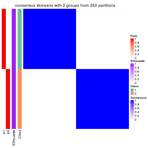
consensus_heatmap(res, k = 3)
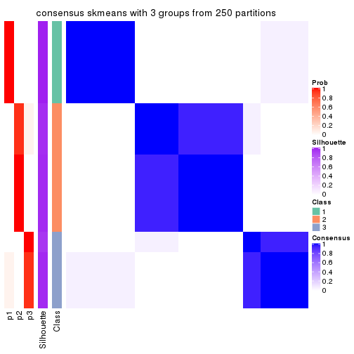
consensus_heatmap(res, k = 4)
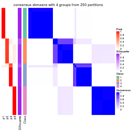
consensus_heatmap(res, k = 5)
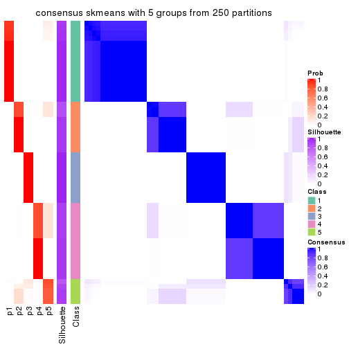
consensus_heatmap(res, k = 6)
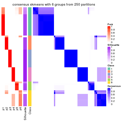
Heatmaps for the membership of samples in all partitions to see how consistent they are:
membership_heatmap(res, k = 2)

membership_heatmap(res, k = 3)
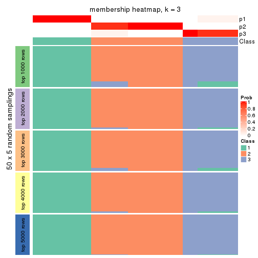
membership_heatmap(res, k = 4)
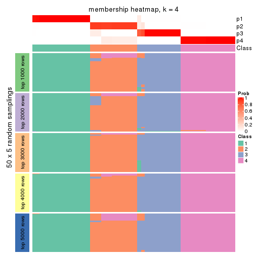
membership_heatmap(res, k = 5)
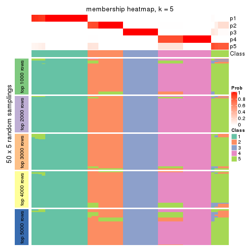
membership_heatmap(res, k = 6)
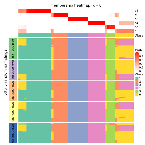
As soon as we have had the classes for columns, we can look for signatures which are significantly different between classes which can be candidate marks for certain classes. Following are the heatmaps for signatures.
Signature heatmaps where rows are scaled:
get_signatures(res, k = 2)

get_signatures(res, k = 3)
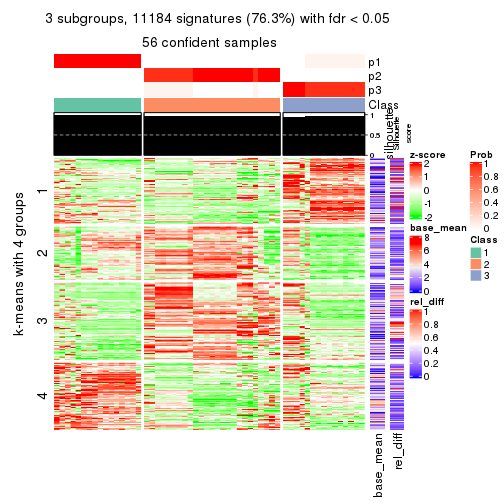
get_signatures(res, k = 4)
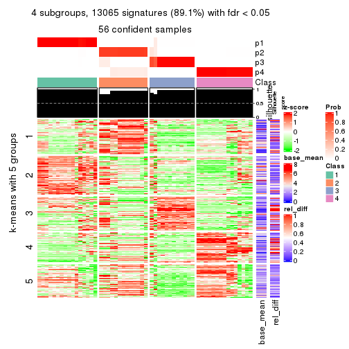
get_signatures(res, k = 5)
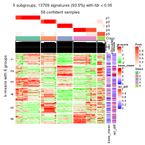
get_signatures(res, k = 6)
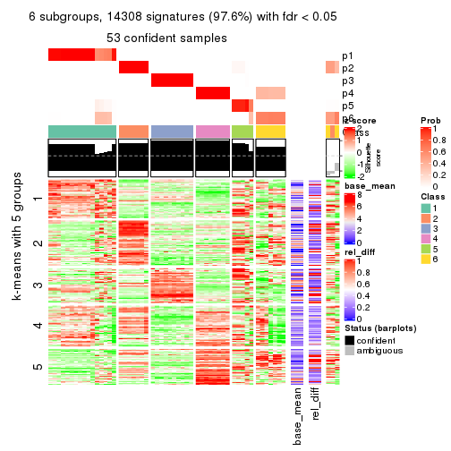
Signature heatmaps where rows are not scaled:
get_signatures(res, k = 2, scale_rows = FALSE)

get_signatures(res, k = 3, scale_rows = FALSE)
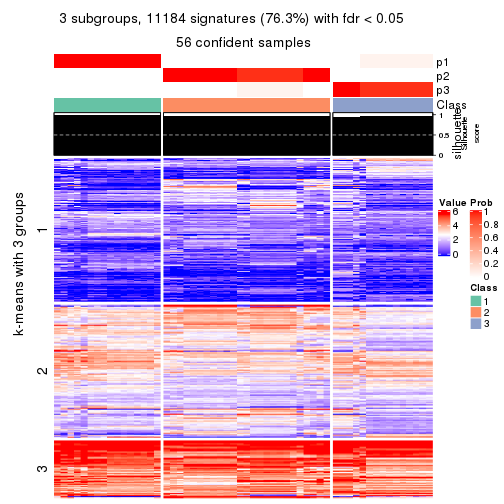
get_signatures(res, k = 4, scale_rows = FALSE)
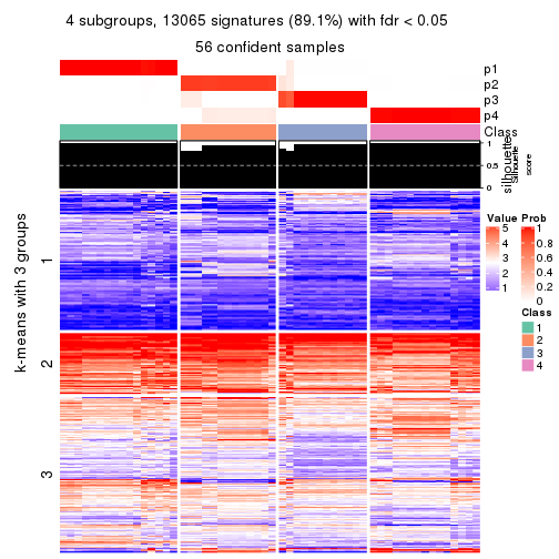
get_signatures(res, k = 5, scale_rows = FALSE)
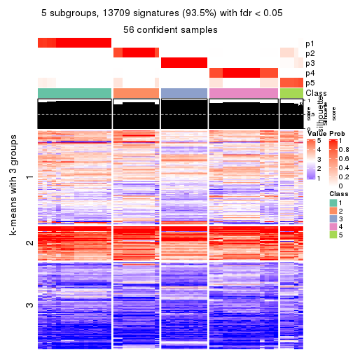
get_signatures(res, k = 6, scale_rows = FALSE)
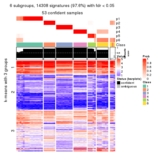
Compare the overlap of signatures from different k:
compare_signatures(res)
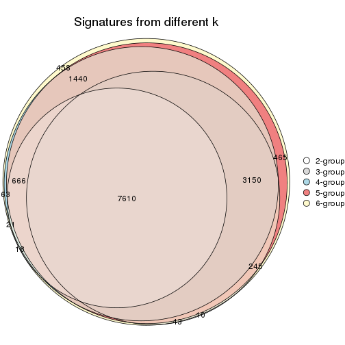
get_signature() returns a data frame invisibly. TO get the list of signatures, the function
call should be assigned to a variable explicitly. In following code, if plot argument is set
to FALSE, no heatmap is plotted while only the differential analysis is performed.
# code only for demonstration
tb = get_signature(res, k = ..., plot = FALSE)
An example of the output of tb is:
#>   which_row         fdr    mean_1    mean_2 scaled_mean_1 scaled_mean_2 km
#> 1        38 0.042760348  8.373488  9.131774    -0.5533452     0.5164555  1
#> 2        40 0.018707592  7.106213  8.469186    -0.6173731     0.5762149  1
#> 3        55 0.019134737 10.221463 11.207825    -0.6159697     0.5749050  1
#> 4        59 0.006059896  5.921854  7.869574    -0.6899429     0.6439467  1
#> 5        60 0.018055526  8.928898 10.211722    -0.6204761     0.5791110  1
#> 6        98 0.009384629 15.714769 14.887706     0.6635654    -0.6193277  2
...
The columns in tb are:
which_row: row indices corresponding to the input matrix.fdr: FDR for the differential test. mean_x: The mean value in group x.scaled_mean_x: The mean value in group x after rows are scaled.km: Row groups if k-means clustering is applied to rows.UMAP plot which shows how samples are separated.
dimension_reduction(res, k = 2, method = "UMAP")

dimension_reduction(res, k = 3, method = "UMAP")
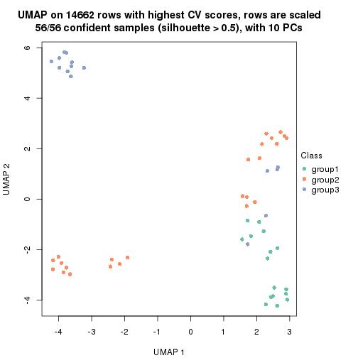
dimension_reduction(res, k = 4, method = "UMAP")
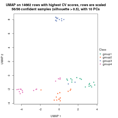
dimension_reduction(res, k = 5, method = "UMAP")
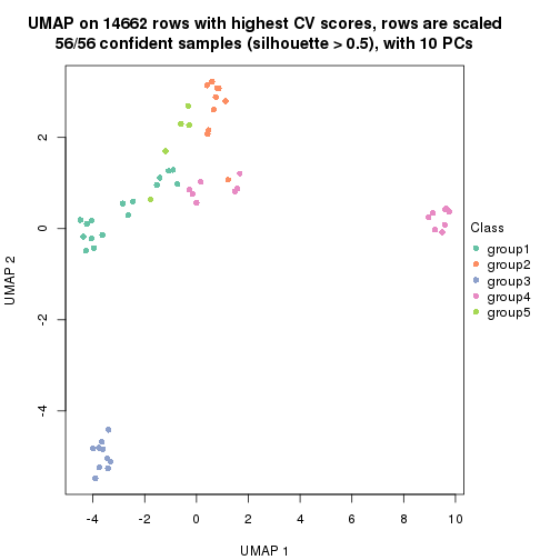
dimension_reduction(res, k = 6, method = "UMAP")

Following heatmap shows how subgroups are split when increasing k:
collect_classes(res)
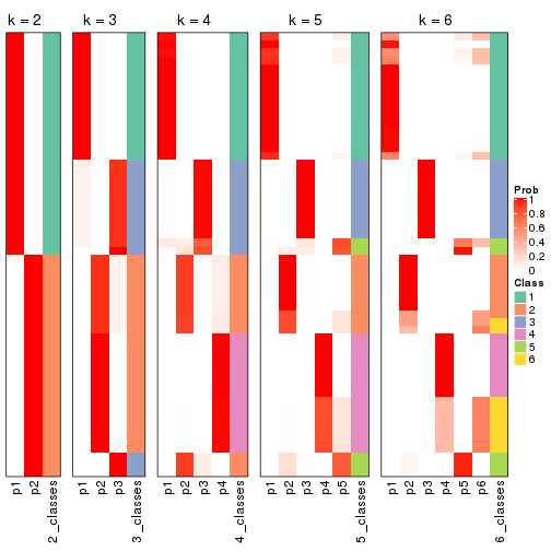
If matrix rows can be associated to genes, consider to use functional_enrichment(res,
...) to perform function enrichment for the signature genes. See this vignette for more detailed explanations.
The object with results only for a single top-value method and a single partition method can be extracted as:
res = res_list["CV", "pam"]
# you can also extract it by
# res = res_list["CV:pam"]
A summary of res and all the functions that can be applied to it:
res
#> A 'ConsensusPartition' object with k = 2, 3, 4, 5, 6.
#>   On a matrix with 14662 rows and 56 columns.
#>   Top rows (1000, 2000, 3000, 4000, 5000) are extracted by 'CV' method.
#>   Subgroups are detected by 'pam' method.
#>   Performed in total 1250 partitions by row resampling.
#>   Best k for subgroups seems to be 6.
#>
#> Following methods can be applied to this 'ConsensusPartition' object:
#>  [1] "cola_report"             "collect_classes"         "collect_plots"
#>  [4] "collect_stats"           "colnames"                "compare_signatures"
#>  [7] "consensus_heatmap"       "dimension_reduction"     "functional_enrichment"
#> [10] "get_anno_col"            "get_anno"                "get_classes"
#> [13] "get_consensus"           "get_matrix"              "get_membership"
#> [16] "get_param"               "get_signatures"          "get_stats"
#> [19] "is_best_k"               "is_stable_k"             "membership_heatmap"
#> [22] "ncol"                    "nrow"                    "plot_ecdf"
#> [25] "rownames"                "select_partition_number" "show"
#> [28] "suggest_best_k"          "test_to_known_factors"
collect_plots() function collects all the plots made from res for all k (number of partitions)
into one single page to provide an easy and fast comparison between different k.
collect_plots(res)
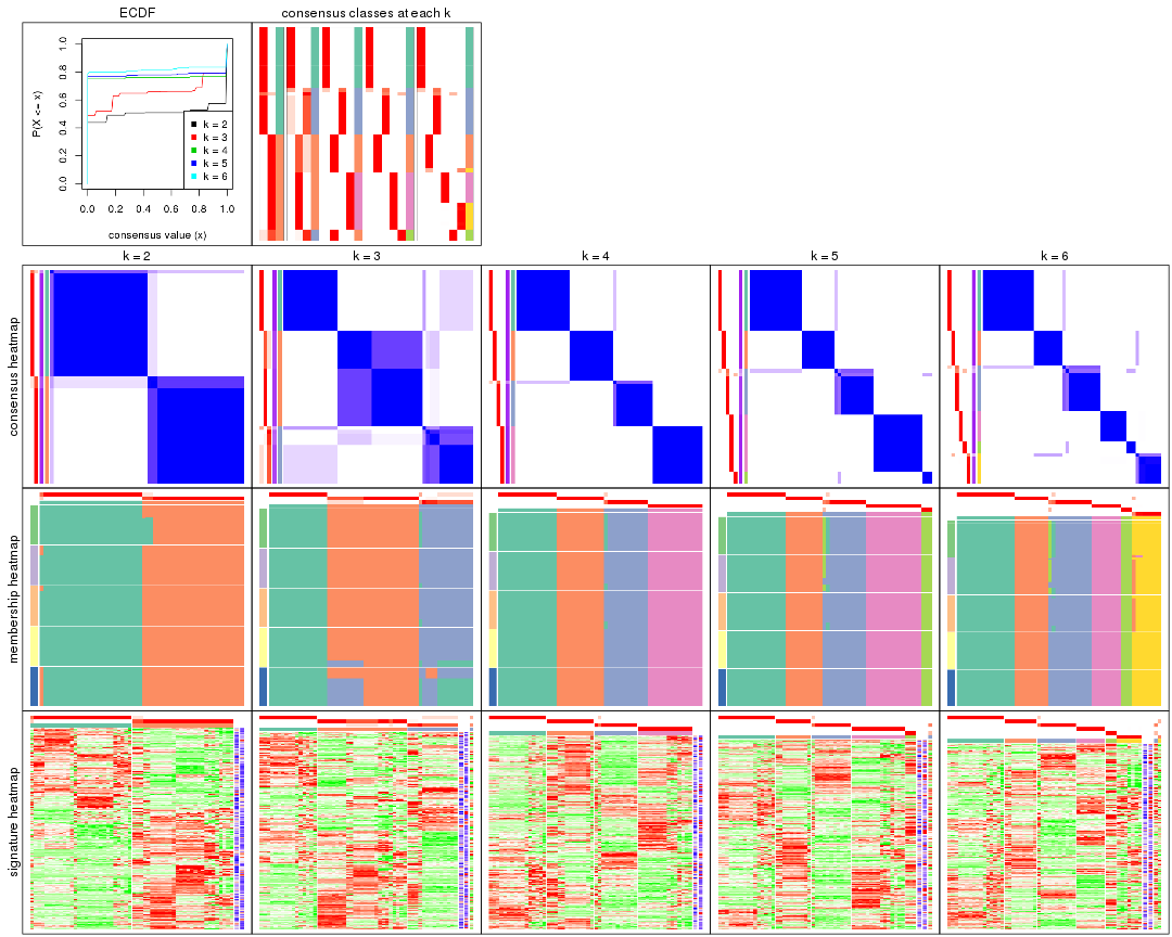
The plots are:
k and the heatmap of
predicted classes for each k.k.k.k.All the plots in panels can be made by individual functions and they are plotted later in this section.
select_partition_number() produces several plots showing different
statistics for choosing “optimized” k. There are following statistics:
k;k, the area increased is defined as \(A_k - A_{k-1}\).The detailed explanations of these statistics can be found in the cola vignette.
Generally speaking, lower PAC score, higher mean silhouette score or higher
concordance corresponds to better partition. Rand index and Jaccard index
measure how similar the current partition is compared to partition with k-1.
If they are too similar, we won't accept k is better than k-1.
select_partition_number(res)
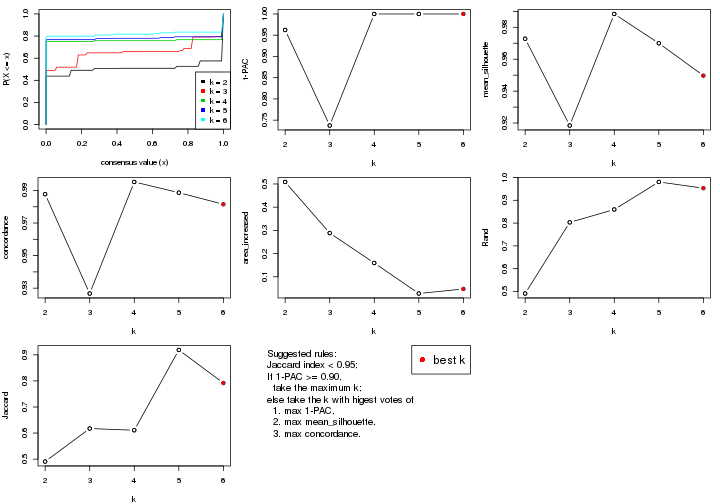
The numeric values for all these statistics can be obtained by get_stats().
get_stats(res)
#>   k 1-PAC mean_silhouette concordance area_increased  Rand Jaccard
#> 2 2 0.962           0.973       0.988         0.5086 0.491   0.491
#> 3 3 0.737           0.918       0.927         0.2884 0.803   0.617
#> 4 4 1.000           0.988       0.995         0.1594 0.860   0.611
#> 5 5 1.000           0.970       0.989         0.0278 0.981   0.919
#> 6 6 1.000           0.950       0.982         0.0475 0.953   0.792
suggest_best_k() suggests the best \(k\) based on these statistics. The rules are as follows:
suggest_best_k(res)
#> [1] 6
#> attr(,"optional")
#> [1] 2 4 5
There is also optional best \(k\) = 2 4 5 that is worth to check.
Following shows the table of the partitions (You need to click the show/hide
code output link to see it). The membership matrix (columns with name p*)
is inferred by
clue::cl_consensus()
function with the SE method. Basically the value in the membership matrix
represents the probability to belong to a certain group. The finall class
label for an item is determined with the group with highest probability it
belongs to.
In get_classes() function, the entropy is calculated from the membership
matrix and the silhouette score is calculated from the consensus matrix.
cbind(get_classes(res, k = 2), get_membership(res, k = 2))
#>           class entropy silhouette    p1    p2
#> SRR073723     1   0.000      0.990 1.000 0.000
#> SRR073724     1   0.000      0.990 1.000 0.000
#> SRR073725     1   0.000      0.990 1.000 0.000
#> SRR073726     2   0.000      0.984 0.000 1.000
#> SRR073727     1   0.000      0.990 1.000 0.000
#> SRR073728     2   0.584      0.846 0.140 0.860
#> SRR073729     2   0.584      0.846 0.140 0.860
#> SRR073730     2   0.574      0.851 0.136 0.864
#> SRR073731     2   0.000      0.984 0.000 1.000
#> SRR073732     2   0.000      0.984 0.000 1.000
#> SRR073733     2   0.000      0.984 0.000 1.000
#> SRR073734     2   0.000      0.984 0.000 1.000
#> SRR073735     2   0.000      0.984 0.000 1.000
#> SRR073736     2   0.000      0.984 0.000 1.000
#> SRR073737     2   0.000      0.984 0.000 1.000
#> SRR073738     1   0.000      0.990 1.000 0.000
#> SRR073739     1   0.000      0.990 1.000 0.000
#> SRR073740     1   0.000      0.990 1.000 0.000
#> SRR073741     1   0.000      0.990 1.000 0.000
#> SRR073742     1   0.000      0.990 1.000 0.000
#> SRR073743     1   0.000      0.990 1.000 0.000
#> SRR073744     1   0.000      0.990 1.000 0.000
#> SRR073745     1   0.000      0.990 1.000 0.000
#> SRR073746     1   0.000      0.990 1.000 0.000
#> SRR073747     1   0.000      0.990 1.000 0.000
#> SRR073748     1   0.000      0.990 1.000 0.000
#> SRR073749     1   0.000      0.990 1.000 0.000
#> SRR073750     1   0.000      0.990 1.000 0.000
#> SRR073751     1   0.844      0.613 0.728 0.272
#> SRR073752     2   0.000      0.984 0.000 1.000
#> SRR073753     2   0.000      0.984 0.000 1.000
#> SRR073754     2   0.000      0.984 0.000 1.000
#> SRR073755     2   0.000      0.984 0.000 1.000
#> SRR073756     2   0.000      0.984 0.000 1.000
#> SRR073758     2   0.000      0.984 0.000 1.000
#> SRR073759     2   0.000      0.984 0.000 1.000
#> SRR073760     2   0.000      0.984 0.000 1.000
#> SRR073761     2   0.000      0.984 0.000 1.000
#> SRR073763     2   0.000      0.984 0.000 1.000
#> SRR073764     2   0.000      0.984 0.000 1.000
#> SRR073765     2   0.000      0.984 0.000 1.000
#> SRR073766     2   0.000      0.984 0.000 1.000
#> SRR073767     2   0.000      0.984 0.000 1.000
#> SRR073768     2   0.000      0.984 0.000 1.000
#> SRR073769     1   0.000      0.990 1.000 0.000
#> SRR073770     1   0.000      0.990 1.000 0.000
#> SRR073771     1   0.000      0.990 1.000 0.000
#> SRR073772     1   0.000      0.990 1.000 0.000
#> SRR073773     1   0.000      0.990 1.000 0.000
#> SRR073774     1   0.000      0.990 1.000 0.000
#> SRR073775     1   0.000      0.990 1.000 0.000
#> SRR073776     1   0.000      0.990 1.000 0.000
#> SRR073777     1   0.000      0.990 1.000 0.000
#> SRR073778     1   0.000      0.990 1.000 0.000
#> SRR073779     2   0.000      0.984 0.000 1.000
#> SRR073780     2   0.000      0.984 0.000 1.000
cbind(get_classes(res, k = 3), get_membership(res, k = 3))
#>           class entropy silhouette    p1    p2    p3
#> SRR073723     3   0.621      0.491 0.428 0.000 0.572
#> SRR073724     1   0.000      1.000 1.000 0.000 0.000
#> SRR073725     1   0.000      1.000 1.000 0.000 0.000
#> SRR073726     2   0.000      0.931 0.000 1.000 0.000
#> SRR073727     1   0.000      1.000 1.000 0.000 0.000
#> SRR073728     3   0.186      0.769 0.000 0.052 0.948
#> SRR073729     3   0.186      0.769 0.000 0.052 0.948
#> SRR073730     3   0.186      0.769 0.000 0.052 0.948
#> SRR073731     2   0.424      0.892 0.000 0.824 0.176
#> SRR073732     2   0.424      0.892 0.000 0.824 0.176
#> SRR073733     2   0.424      0.892 0.000 0.824 0.176
#> SRR073734     2   0.424      0.892 0.000 0.824 0.176
#> SRR073735     2   0.424      0.892 0.000 0.824 0.176
#> SRR073736     2   0.424      0.892 0.000 0.824 0.176
#> SRR073737     2   0.424      0.892 0.000 0.824 0.176
#> SRR073738     1   0.000      1.000 1.000 0.000 0.000
#> SRR073739     1   0.000      1.000 1.000 0.000 0.000
#> SRR073740     1   0.000      1.000 1.000 0.000 0.000
#> SRR073741     1   0.000      1.000 1.000 0.000 0.000
#> SRR073742     1   0.000      1.000 1.000 0.000 0.000
#> SRR073743     1   0.000      1.000 1.000 0.000 0.000
#> SRR073744     1   0.000      1.000 1.000 0.000 0.000
#> SRR073745     1   0.000      1.000 1.000 0.000 0.000
#> SRR073746     1   0.000      1.000 1.000 0.000 0.000
#> SRR073747     1   0.000      1.000 1.000 0.000 0.000
#> SRR073748     1   0.000      1.000 1.000 0.000 0.000
#> SRR073749     1   0.000      1.000 1.000 0.000 0.000
#> SRR073750     1   0.000      1.000 1.000 0.000 0.000
#> SRR073751     3   0.000      0.792 0.000 0.000 1.000
#> SRR073752     2   0.424      0.892 0.000 0.824 0.176
#> SRR073753     2   0.424      0.892 0.000 0.824 0.176
#> SRR073754     2   0.000      0.931 0.000 1.000 0.000
#> SRR073755     2   0.000      0.931 0.000 1.000 0.000
#> SRR073756     2   0.000      0.931 0.000 1.000 0.000
#> SRR073758     2   0.000      0.931 0.000 1.000 0.000
#> SRR073759     2   0.424      0.892 0.000 0.824 0.176
#> SRR073760     2   0.000      0.931 0.000 1.000 0.000
#> SRR073761     2   0.000      0.931 0.000 1.000 0.000
#> SRR073763     2   0.000      0.931 0.000 1.000 0.000
#> SRR073764     2   0.000      0.931 0.000 1.000 0.000
#> SRR073765     2   0.000      0.931 0.000 1.000 0.000
#> SRR073766     2   0.000      0.931 0.000 1.000 0.000
#> SRR073767     2   0.000      0.931 0.000 1.000 0.000
#> SRR073768     2   0.000      0.931 0.000 1.000 0.000
#> SRR073769     3   0.424      0.896 0.176 0.000 0.824
#> SRR073770     3   0.424      0.896 0.176 0.000 0.824
#> SRR073771     3   0.424      0.896 0.176 0.000 0.824
#> SRR073772     3   0.424      0.896 0.176 0.000 0.824
#> SRR073773     3   0.424      0.896 0.176 0.000 0.824
#> SRR073774     3   0.424      0.896 0.176 0.000 0.824
#> SRR073775     3   0.424      0.896 0.176 0.000 0.824
#> SRR073776     3   0.424      0.896 0.176 0.000 0.824
#> SRR073777     3   0.424      0.896 0.176 0.000 0.824
#> SRR073778     3   0.424      0.896 0.176 0.000 0.824
#> SRR073779     2   0.000      0.931 0.000 1.000 0.000
#> SRR073780     2   0.000      0.931 0.000 1.000 0.000
cbind(get_classes(res, k = 4), get_membership(res, k = 4))
#>           class entropy silhouette    p1 p2    p3 p4
#> SRR073723     3   0.419      0.634 0.268  0 0.732  0
#> SRR073724     1   0.000      1.000 1.000  0 0.000  0
#> SRR073725     1   0.000      1.000 1.000  0 0.000  0
#> SRR073726     4   0.000      1.000 0.000  0 0.000  1
#> SRR073727     1   0.000      1.000 1.000  0 0.000  0
#> SRR073728     2   0.000      1.000 0.000  1 0.000  0
#> SRR073729     2   0.000      1.000 0.000  1 0.000  0
#> SRR073730     2   0.000      1.000 0.000  1 0.000  0
#> SRR073731     2   0.000      1.000 0.000  1 0.000  0
#> SRR073732     2   0.000      1.000 0.000  1 0.000  0
#> SRR073733     2   0.000      1.000 0.000  1 0.000  0
#> SRR073734     2   0.000      1.000 0.000  1 0.000  0
#> SRR073735     2   0.000      1.000 0.000  1 0.000  0
#> SRR073736     2   0.000      1.000 0.000  1 0.000  0
#> SRR073737     2   0.000      1.000 0.000  1 0.000  0
#> SRR073738     1   0.000      1.000 1.000  0 0.000  0
#> SRR073739     1   0.000      1.000 1.000  0 0.000  0
#> SRR073740     1   0.000      1.000 1.000  0 0.000  0
#> SRR073741     1   0.000      1.000 1.000  0 0.000  0
#> SRR073742     1   0.000      1.000 1.000  0 0.000  0
#> SRR073743     1   0.000      1.000 1.000  0 0.000  0
#> SRR073744     1   0.000      1.000 1.000  0 0.000  0
#> SRR073745     1   0.000      1.000 1.000  0 0.000  0
#> SRR073746     1   0.000      1.000 1.000  0 0.000  0
#> SRR073747     1   0.000      1.000 1.000  0 0.000  0
#> SRR073748     1   0.000      1.000 1.000  0 0.000  0
#> SRR073749     1   0.000      1.000 1.000  0 0.000  0
#> SRR073750     1   0.000      1.000 1.000  0 0.000  0
#> SRR073751     3   0.000      0.974 0.000  0 1.000  0
#> SRR073752     2   0.000      1.000 0.000  1 0.000  0
#> SRR073753     2   0.000      1.000 0.000  1 0.000  0
#> SRR073754     4   0.000      1.000 0.000  0 0.000  1
#> SRR073755     4   0.000      1.000 0.000  0 0.000  1
#> SRR073756     4   0.000      1.000 0.000  0 0.000  1
#> SRR073758     4   0.000      1.000 0.000  0 0.000  1
#> SRR073759     2   0.000      1.000 0.000  1 0.000  0
#> SRR073760     4   0.000      1.000 0.000  0 0.000  1
#> SRR073761     4   0.000      1.000 0.000  0 0.000  1
#> SRR073763     4   0.000      1.000 0.000  0 0.000  1
#> SRR073764     4   0.000      1.000 0.000  0 0.000  1
#> SRR073765     4   0.000      1.000 0.000  0 0.000  1
#> SRR073766     4   0.000      1.000 0.000  0 0.000  1
#> SRR073767     4   0.000      1.000 0.000  0 0.000  1
#> SRR073768     4   0.000      1.000 0.000  0 0.000  1
#> SRR073769     3   0.000      0.974 0.000  0 1.000  0
#> SRR073770     3   0.000      0.974 0.000  0 1.000  0
#> SRR073771     3   0.000      0.974 0.000  0 1.000  0
#> SRR073772     3   0.000      0.974 0.000  0 1.000  0
#> SRR073773     3   0.000      0.974 0.000  0 1.000  0
#> SRR073774     3   0.000      0.974 0.000  0 1.000  0
#> SRR073775     3   0.000      0.974 0.000  0 1.000  0
#> SRR073776     3   0.000      0.974 0.000  0 1.000  0
#> SRR073777     3   0.000      0.974 0.000  0 1.000  0
#> SRR073778     3   0.000      0.974 0.000  0 1.000  0
#> SRR073779     4   0.000      1.000 0.000  0 0.000  1
#> SRR073780     4   0.000      1.000 0.000  0 0.000  1
cbind(get_classes(res, k = 5), get_membership(res, k = 5))
#>           class entropy silhouette    p1 p2    p3 p4   p5
#> SRR073723     3   0.366      0.558 0.276  0 0.724  0 0.00
#> SRR073724     1   0.000      1.000 1.000  0 0.000  0 0.00
#> SRR073725     1   0.000      1.000 1.000  0 0.000  0 0.00
#> SRR073726     4   0.000      1.000 0.000  0 0.000  1 0.00
#> SRR073727     1   0.000      1.000 1.000  0 0.000  0 0.00
#> SRR073728     5   0.000      1.000 0.000  0 0.000  0 1.00
#> SRR073729     5   0.000      1.000 0.000  0 0.000  0 1.00
#> SRR073730     5   0.000      1.000 0.000  0 0.000  0 1.00
#> SRR073731     2   0.000      1.000 0.000  1 0.000  0 0.00
#> SRR073732     2   0.000      1.000 0.000  1 0.000  0 0.00
#> SRR073733     2   0.000      1.000 0.000  1 0.000  0 0.00
#> SRR073734     2   0.000      1.000 0.000  1 0.000  0 0.00
#> SRR073735     2   0.000      1.000 0.000  1 0.000  0 0.00
#> SRR073736     2   0.000      1.000 0.000  1 0.000  0 0.00
#> SRR073737     2   0.000      1.000 0.000  1 0.000  0 0.00
#> SRR073738     1   0.000      1.000 1.000  0 0.000  0 0.00
#> SRR073739     1   0.000      1.000 1.000  0 0.000  0 0.00
#> SRR073740     1   0.000      1.000 1.000  0 0.000  0 0.00
#> SRR073741     1   0.000      1.000 1.000  0 0.000  0 0.00
#> SRR073742     1   0.000      1.000 1.000  0 0.000  0 0.00
#> SRR073743     1   0.000      1.000 1.000  0 0.000  0 0.00
#> SRR073744     1   0.000      1.000 1.000  0 0.000  0 0.00
#> SRR073745     1   0.000      1.000 1.000  0 0.000  0 0.00
#> SRR073746     1   0.000      1.000 1.000  0 0.000  0 0.00
#> SRR073747     1   0.000      1.000 1.000  0 0.000  0 0.00
#> SRR073748     1   0.000      1.000 1.000  0 0.000  0 0.00
#> SRR073749     1   0.000      1.000 1.000  0 0.000  0 0.00
#> SRR073750     1   0.000      1.000 1.000  0 0.000  0 0.00
#> SRR073751     3   0.406      0.449 0.000  0 0.640  0 0.36
#> SRR073752     2   0.000      1.000 0.000  1 0.000  0 0.00
#> SRR073753     2   0.000      1.000 0.000  1 0.000  0 0.00
#> SRR073754     4   0.000      1.000 0.000  0 0.000  1 0.00
#> SRR073755     4   0.000      1.000 0.000  0 0.000  1 0.00
#> SRR073756     4   0.000      1.000 0.000  0 0.000  1 0.00
#> SRR073758     4   0.000      1.000 0.000  0 0.000  1 0.00
#> SRR073759     2   0.000      1.000 0.000  1 0.000  0 0.00
#> SRR073760     4   0.000      1.000 0.000  0 0.000  1 0.00
#> SRR073761     4   0.000      1.000 0.000  0 0.000  1 0.00
#> SRR073763     4   0.000      1.000 0.000  0 0.000  1 0.00
#> SRR073764     4   0.000      1.000 0.000  0 0.000  1 0.00
#> SRR073765     4   0.000      1.000 0.000  0 0.000  1 0.00
#> SRR073766     4   0.000      1.000 0.000  0 0.000  1 0.00
#> SRR073767     4   0.000      1.000 0.000  0 0.000  1 0.00
#> SRR073768     4   0.000      1.000 0.000  0 0.000  1 0.00
#> SRR073769     3   0.000      0.931 0.000  0 1.000  0 0.00
#> SRR073770     3   0.000      0.931 0.000  0 1.000  0 0.00
#> SRR073771     3   0.000      0.931 0.000  0 1.000  0 0.00
#> SRR073772     3   0.000      0.931 0.000  0 1.000  0 0.00
#> SRR073773     3   0.000      0.931 0.000  0 1.000  0 0.00
#> SRR073774     3   0.000      0.931 0.000  0 1.000  0 0.00
#> SRR073775     3   0.000      0.931 0.000  0 1.000  0 0.00
#> SRR073776     3   0.000      0.931 0.000  0 1.000  0 0.00
#> SRR073777     3   0.000      0.931 0.000  0 1.000  0 0.00
#> SRR073778     3   0.000      0.931 0.000  0 1.000  0 0.00
#> SRR073779     4   0.000      1.000 0.000  0 0.000  1 0.00
#> SRR073780     4   0.000      1.000 0.000  0 0.000  1 0.00
cbind(get_classes(res, k = 6), get_membership(res, k = 6))
#>           class entropy silhouette    p1    p2    p3    p4   p5    p6
#> SRR073723     3   0.329      0.558 0.276 0.000 0.724 0.000 0.00 0.000
#> SRR073724     1   0.000      1.000 1.000 0.000 0.000 0.000 0.00 0.000
#> SRR073725     1   0.000      1.000 1.000 0.000 0.000 0.000 0.00 0.000
#> SRR073726     6   0.000      0.928 0.000 0.000 0.000 0.000 0.00 1.000
#> SRR073727     1   0.000      1.000 1.000 0.000 0.000 0.000 0.00 0.000
#> SRR073728     5   0.000      1.000 0.000 0.000 0.000 0.000 1.00 0.000
#> SRR073729     5   0.000      1.000 0.000 0.000 0.000 0.000 1.00 0.000
#> SRR073730     5   0.000      1.000 0.000 0.000 0.000 0.000 1.00 0.000
#> SRR073731     2   0.000      1.000 0.000 1.000 0.000 0.000 0.00 0.000
#> SRR073732     2   0.000      1.000 0.000 1.000 0.000 0.000 0.00 0.000
#> SRR073733     2   0.000      1.000 0.000 1.000 0.000 0.000 0.00 0.000
#> SRR073734     2   0.000      1.000 0.000 1.000 0.000 0.000 0.00 0.000
#> SRR073735     2   0.000      1.000 0.000 1.000 0.000 0.000 0.00 0.000
#> SRR073736     2   0.000      1.000 0.000 1.000 0.000 0.000 0.00 0.000
#> SRR073737     2   0.000      1.000 0.000 1.000 0.000 0.000 0.00 0.000
#> SRR073738     1   0.000      1.000 1.000 0.000 0.000 0.000 0.00 0.000
#> SRR073739     1   0.000      1.000 1.000 0.000 0.000 0.000 0.00 0.000
#> SRR073740     1   0.000      1.000 1.000 0.000 0.000 0.000 0.00 0.000
#> SRR073741     1   0.000      1.000 1.000 0.000 0.000 0.000 0.00 0.000
#> SRR073742     1   0.000      1.000 1.000 0.000 0.000 0.000 0.00 0.000
#> SRR073743     1   0.000      1.000 1.000 0.000 0.000 0.000 0.00 0.000
#> SRR073744     1   0.000      1.000 1.000 0.000 0.000 0.000 0.00 0.000
#> SRR073745     1   0.000      1.000 1.000 0.000 0.000 0.000 0.00 0.000
#> SRR073746     1   0.000      1.000 1.000 0.000 0.000 0.000 0.00 0.000
#> SRR073747     1   0.000      1.000 1.000 0.000 0.000 0.000 0.00 0.000
#> SRR073748     1   0.000      1.000 1.000 0.000 0.000 0.000 0.00 0.000
#> SRR073749     1   0.000      1.000 1.000 0.000 0.000 0.000 0.00 0.000
#> SRR073750     1   0.000      1.000 1.000 0.000 0.000 0.000 0.00 0.000
#> SRR073751     3   0.365      0.449 0.000 0.000 0.640 0.000 0.36 0.000
#> SRR073752     2   0.000      1.000 0.000 1.000 0.000 0.000 0.00 0.000
#> SRR073753     2   0.000      1.000 0.000 1.000 0.000 0.000 0.00 0.000
#> SRR073754     6   0.026      0.924 0.000 0.000 0.000 0.008 0.00 0.992
#> SRR073755     6   0.000      0.928 0.000 0.000 0.000 0.000 0.00 1.000
#> SRR073756     6   0.000      0.928 0.000 0.000 0.000 0.000 0.00 1.000
#> SRR073758     6   0.000      0.928 0.000 0.000 0.000 0.000 0.00 1.000
#> SRR073759     6   0.372      0.379 0.000 0.384 0.000 0.000 0.00 0.616
#> SRR073760     4   0.000      1.000 0.000 0.000 0.000 1.000 0.00 0.000
#> SRR073761     4   0.000      1.000 0.000 0.000 0.000 1.000 0.00 0.000
#> SRR073763     4   0.000      1.000 0.000 0.000 0.000 1.000 0.00 0.000
#> SRR073764     4   0.000      1.000 0.000 0.000 0.000 1.000 0.00 0.000
#> SRR073765     4   0.000      1.000 0.000 0.000 0.000 1.000 0.00 0.000
#> SRR073766     4   0.000      1.000 0.000 0.000 0.000 1.000 0.00 0.000
#> SRR073767     4   0.000      1.000 0.000 0.000 0.000 1.000 0.00 0.000
#> SRR073768     4   0.000      1.000 0.000 0.000 0.000 1.000 0.00 0.000
#> SRR073769     3   0.000      0.931 0.000 0.000 1.000 0.000 0.00 0.000
#> SRR073770     3   0.000      0.931 0.000 0.000 1.000 0.000 0.00 0.000
#> SRR073771     3   0.000      0.931 0.000 0.000 1.000 0.000 0.00 0.000
#> SRR073772     3   0.000      0.931 0.000 0.000 1.000 0.000 0.00 0.000
#> SRR073773     3   0.000      0.931 0.000 0.000 1.000 0.000 0.00 0.000
#> SRR073774     3   0.000      0.931 0.000 0.000 1.000 0.000 0.00 0.000
#> SRR073775     3   0.000      0.931 0.000 0.000 1.000 0.000 0.00 0.000
#> SRR073776     3   0.000      0.931 0.000 0.000 1.000 0.000 0.00 0.000
#> SRR073777     3   0.000      0.931 0.000 0.000 1.000 0.000 0.00 0.000
#> SRR073778     3   0.000      0.931 0.000 0.000 1.000 0.000 0.00 0.000
#> SRR073779     6   0.026      0.924 0.000 0.000 0.000 0.008 0.00 0.992
#> SRR073780     6   0.000      0.928 0.000 0.000 0.000 0.000 0.00 1.000
Heatmaps for the consensus matrix. It visualizes the probability of two samples to be in a same group.
consensus_heatmap(res, k = 2)

consensus_heatmap(res, k = 3)
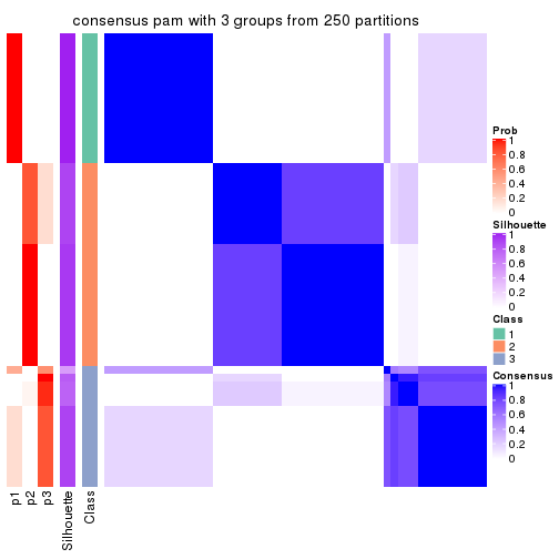
consensus_heatmap(res, k = 4)
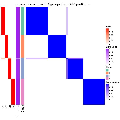
consensus_heatmap(res, k = 5)
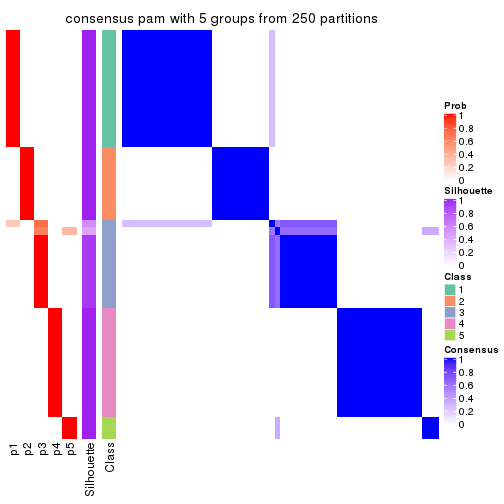
consensus_heatmap(res, k = 6)
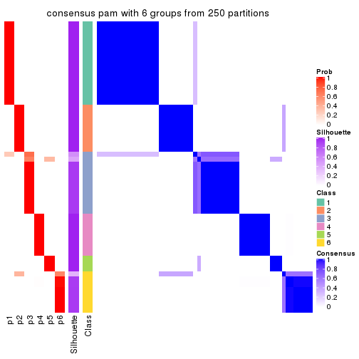
Heatmaps for the membership of samples in all partitions to see how consistent they are:
membership_heatmap(res, k = 2)

membership_heatmap(res, k = 3)
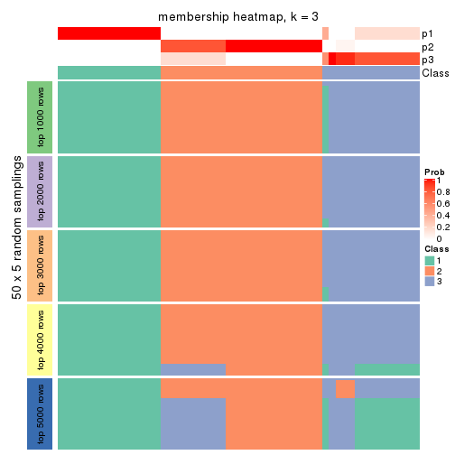
membership_heatmap(res, k = 4)
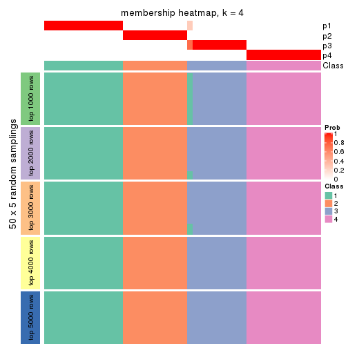
membership_heatmap(res, k = 5)
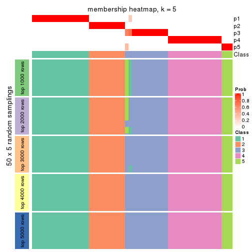
membership_heatmap(res, k = 6)
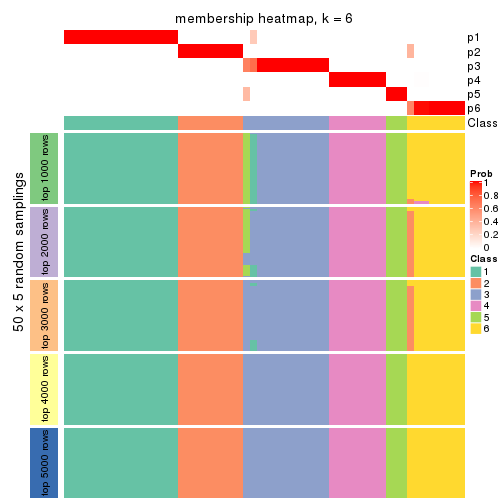
As soon as we have had the classes for columns, we can look for signatures which are significantly different between classes which can be candidate marks for certain classes. Following are the heatmaps for signatures.
Signature heatmaps where rows are scaled:
get_signatures(res, k = 2)

get_signatures(res, k = 3)
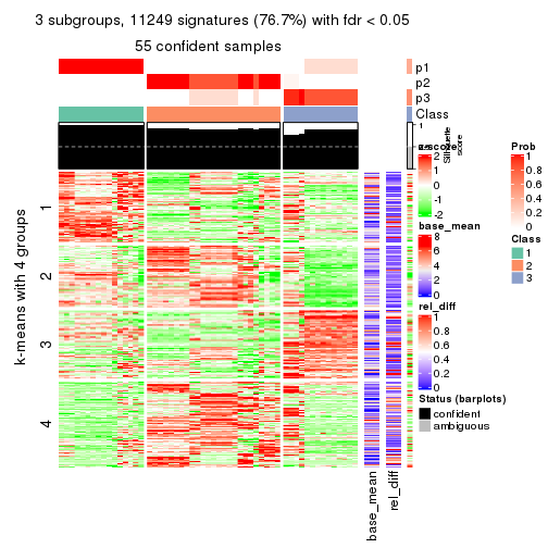
get_signatures(res, k = 4)
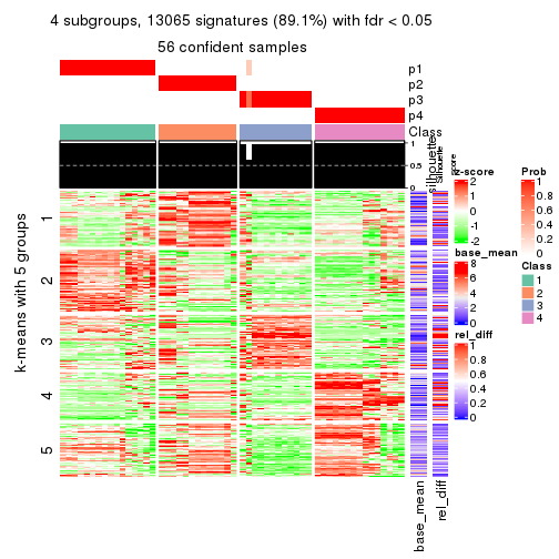
get_signatures(res, k = 5)
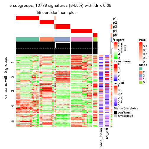
get_signatures(res, k = 6)
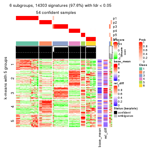
Signature heatmaps where rows are not scaled:
get_signatures(res, k = 2, scale_rows = FALSE)

get_signatures(res, k = 3, scale_rows = FALSE)
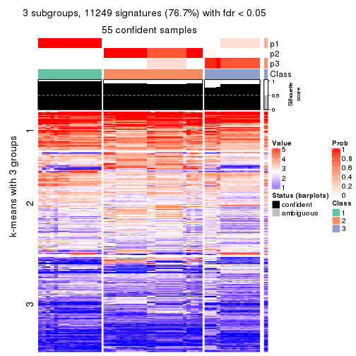
get_signatures(res, k = 4, scale_rows = FALSE)
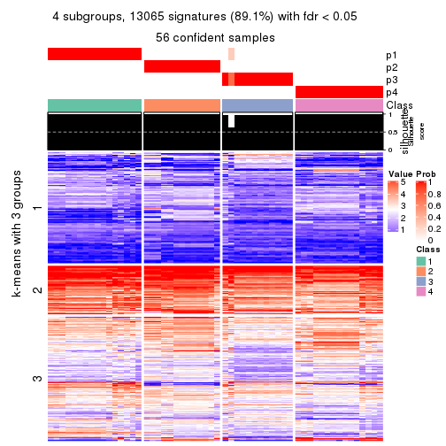
get_signatures(res, k = 5, scale_rows = FALSE)
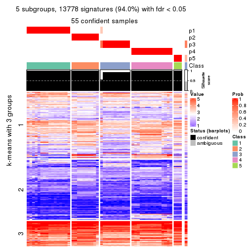
get_signatures(res, k = 6, scale_rows = FALSE)
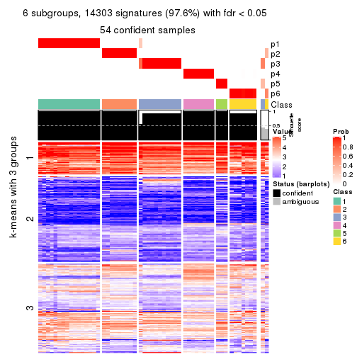
Compare the overlap of signatures from different k:
compare_signatures(res)
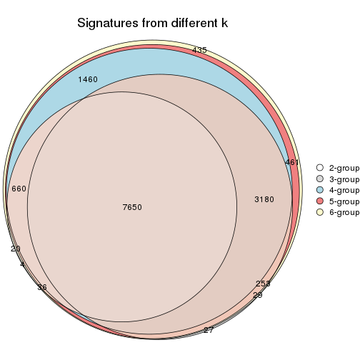
get_signature() returns a data frame invisibly. TO get the list of signatures, the function
call should be assigned to a variable explicitly. In following code, if plot argument is set
to FALSE, no heatmap is plotted while only the differential analysis is performed.
# code only for demonstration
tb = get_signature(res, k = ..., plot = FALSE)
An example of the output of tb is:
#>   which_row         fdr    mean_1    mean_2 scaled_mean_1 scaled_mean_2 km
#> 1        38 0.042760348  8.373488  9.131774    -0.5533452     0.5164555  1
#> 2        40 0.018707592  7.106213  8.469186    -0.6173731     0.5762149  1
#> 3        55 0.019134737 10.221463 11.207825    -0.6159697     0.5749050  1
#> 4        59 0.006059896  5.921854  7.869574    -0.6899429     0.6439467  1
#> 5        60 0.018055526  8.928898 10.211722    -0.6204761     0.5791110  1
#> 6        98 0.009384629 15.714769 14.887706     0.6635654    -0.6193277  2
...
The columns in tb are:
which_row: row indices corresponding to the input matrix.fdr: FDR for the differential test. mean_x: The mean value in group x.scaled_mean_x: The mean value in group x after rows are scaled.km: Row groups if k-means clustering is applied to rows.UMAP plot which shows how samples are separated.
dimension_reduction(res, k = 2, method = "UMAP")

dimension_reduction(res, k = 3, method = "UMAP")
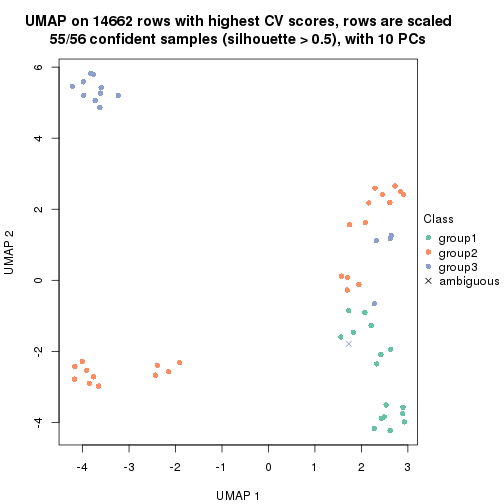
dimension_reduction(res, k = 4, method = "UMAP")

dimension_reduction(res, k = 5, method = "UMAP")

dimension_reduction(res, k = 6, method = "UMAP")
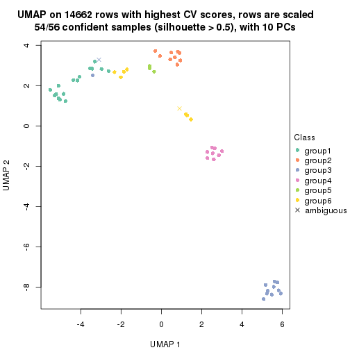
Following heatmap shows how subgroups are split when increasing k:
collect_classes(res)
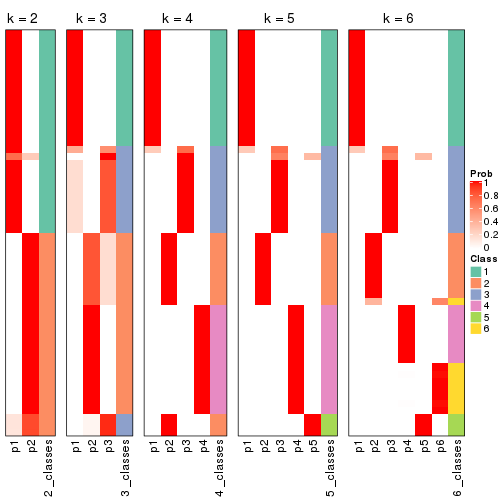
If matrix rows can be associated to genes, consider to use functional_enrichment(res,
...) to perform function enrichment for the signature genes. See this vignette for more detailed explanations.
The object with results only for a single top-value method and a single partition method can be extracted as:
res = res_list["CV", "mclust"]
# you can also extract it by
# res = res_list["CV:mclust"]
A summary of res and all the functions that can be applied to it:
res
#> A 'ConsensusPartition' object with k = 2, 3, 4, 5, 6.
#>   On a matrix with 14662 rows and 56 columns.
#>   Top rows (1000, 2000, 3000, 4000, 5000) are extracted by 'CV' method.
#>   Subgroups are detected by 'mclust' method.
#>   Performed in total 1250 partitions by row resampling.
#>   Best k for subgroups seems to be 6.
#>
#> Following methods can be applied to this 'ConsensusPartition' object:
#>  [1] "cola_report"             "collect_classes"         "collect_plots"
#>  [4] "collect_stats"           "colnames"                "compare_signatures"
#>  [7] "consensus_heatmap"       "dimension_reduction"     "functional_enrichment"
#> [10] "get_anno_col"            "get_anno"                "get_classes"
#> [13] "get_consensus"           "get_matrix"              "get_membership"
#> [16] "get_param"               "get_signatures"          "get_stats"
#> [19] "is_best_k"               "is_stable_k"             "membership_heatmap"
#> [22] "ncol"                    "nrow"                    "plot_ecdf"
#> [25] "rownames"                "select_partition_number" "show"
#> [28] "suggest_best_k"          "test_to_known_factors"
collect_plots() function collects all the plots made from res for all k (number of partitions)
into one single page to provide an easy and fast comparison between different k.
collect_plots(res)
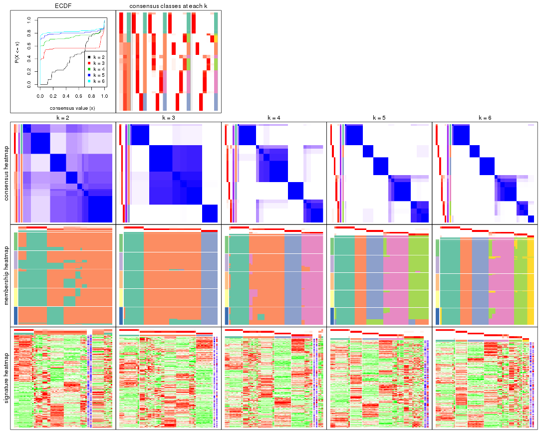
The plots are:
k and the heatmap of
predicted classes for each k.k.k.k.All the plots in panels can be made by individual functions and they are plotted later in this section.
select_partition_number() produces several plots showing different
statistics for choosing “optimized” k. There are following statistics:
k;k, the area increased is defined as \(A_k - A_{k-1}\).The detailed explanations of these statistics can be found in the cola vignette.
Generally speaking, lower PAC score, higher mean silhouette score or higher
concordance corresponds to better partition. Rand index and Jaccard index
measure how similar the current partition is compared to partition with k-1.
If they are too similar, we won't accept k is better than k-1.
select_partition_number(res)
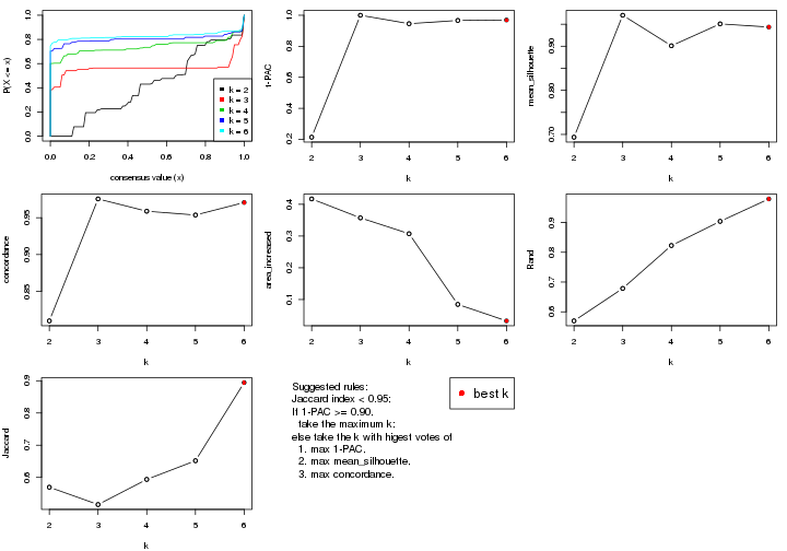
The numeric values for all these statistics can be obtained by get_stats().
get_stats(res)
#>   k 1-PAC mean_silhouette concordance area_increased  Rand Jaccard
#> 2 2 0.214           0.694       0.810         0.4169 0.569   0.569
#> 3 3 1.000           0.970       0.976         0.3572 0.679   0.516
#> 4 4 0.946           0.901       0.959         0.3073 0.823   0.594
#> 5 5 0.967           0.951       0.954         0.0846 0.904   0.652
#> 6 6 0.970           0.944       0.971         0.0326 0.979   0.894
suggest_best_k() suggests the best \(k\) based on these statistics. The rules are as follows:
suggest_best_k(res)
#> [1] 6
#> attr(,"optional")
#> [1] 3 4 5
There is also optional best \(k\) = 3 4 5 that is worth to check.
Following shows the table of the partitions (You need to click the show/hide
code output link to see it). The membership matrix (columns with name p*)
is inferred by
clue::cl_consensus()
function with the SE method. Basically the value in the membership matrix
represents the probability to belong to a certain group. The finall class
label for an item is determined with the group with highest probability it
belongs to.
In get_classes() function, the entropy is calculated from the membership
matrix and the silhouette score is calculated from the consensus matrix.
cbind(get_classes(res, k = 2), get_membership(res, k = 2))
#>           class entropy silhouette    p1    p2
#> SRR073723     1   0.855      0.467 0.720 0.280
#> SRR073724     1   0.855      0.467 0.720 0.280
#> SRR073725     1   0.000      0.857 1.000 0.000
#> SRR073726     2   0.671      0.785 0.176 0.824
#> SRR073727     1   0.866      0.455 0.712 0.288
#> SRR073728     2   0.949      0.561 0.368 0.632
#> SRR073729     2   0.949      0.561 0.368 0.632
#> SRR073730     2   0.949      0.561 0.368 0.632
#> SRR073731     2   0.981      0.487 0.420 0.580
#> SRR073732     2   0.981      0.487 0.420 0.580
#> SRR073733     2   0.981      0.487 0.420 0.580
#> SRR073734     2   0.981      0.487 0.420 0.580
#> SRR073735     2   0.981      0.487 0.420 0.580
#> SRR073736     2   0.981      0.487 0.420 0.580
#> SRR073737     2   0.981      0.487 0.420 0.580
#> SRR073738     1   0.866      0.455 0.712 0.288
#> SRR073739     1   0.000      0.857 1.000 0.000
#> SRR073740     1   0.000      0.857 1.000 0.000
#> SRR073741     1   0.000      0.857 1.000 0.000
#> SRR073742     1   0.000      0.857 1.000 0.000
#> SRR073743     1   0.000      0.857 1.000 0.000
#> SRR073744     1   0.000      0.857 1.000 0.000
#> SRR073745     1   0.000      0.857 1.000 0.000
#> SRR073746     1   0.000      0.857 1.000 0.000
#> SRR073747     1   0.000      0.857 1.000 0.000
#> SRR073748     1   0.000      0.857 1.000 0.000
#> SRR073749     1   0.000      0.857 1.000 0.000
#> SRR073750     1   0.855      0.467 0.720 0.280
#> SRR073751     2   0.827      0.745 0.260 0.740
#> SRR073752     2   0.795      0.747 0.240 0.760
#> SRR073753     2   0.795      0.747 0.240 0.760
#> SRR073754     2   0.671      0.785 0.176 0.824
#> SRR073755     2   0.671      0.785 0.176 0.824
#> SRR073756     2   0.671      0.785 0.176 0.824
#> SRR073758     2   0.671      0.785 0.176 0.824
#> SRR073759     2   0.795      0.747 0.240 0.760
#> SRR073760     2   0.671      0.785 0.176 0.824
#> SRR073761     2   0.671      0.785 0.176 0.824
#> SRR073763     2   0.671      0.785 0.176 0.824
#> SRR073764     2   0.671      0.785 0.176 0.824
#> SRR073765     2   0.671      0.785 0.176 0.824
#> SRR073766     2   0.671      0.785 0.176 0.824
#> SRR073767     2   0.671      0.785 0.176 0.824
#> SRR073768     2   0.671      0.785 0.176 0.824
#> SRR073769     2   0.529      0.640 0.120 0.880
#> SRR073770     2   0.529      0.640 0.120 0.880
#> SRR073771     2   0.529      0.640 0.120 0.880
#> SRR073772     2   0.529      0.640 0.120 0.880
#> SRR073773     2   0.529      0.640 0.120 0.880
#> SRR073774     2   0.529      0.640 0.120 0.880
#> SRR073775     2   0.529      0.640 0.120 0.880
#> SRR073776     2   0.529      0.640 0.120 0.880
#> SRR073777     2   0.529      0.640 0.120 0.880
#> SRR073778     2   0.529      0.640 0.120 0.880
#> SRR073779     2   0.671      0.785 0.176 0.824
#> SRR073780     2   0.671      0.785 0.176 0.824
cbind(get_classes(res, k = 3), get_membership(res, k = 3))
#>           class entropy silhouette    p1    p2    p3
#> SRR073723     2   0.254      0.955 0.080 0.920 0.000
#> SRR073724     2   0.254      0.955 0.080 0.920 0.000
#> SRR073725     1   0.362      0.795 0.864 0.136 0.000
#> SRR073726     2   0.000      0.963 0.000 1.000 0.000
#> SRR073727     2   0.254      0.955 0.080 0.920 0.000
#> SRR073728     2   0.255      0.964 0.056 0.932 0.012
#> SRR073729     2   0.255      0.964 0.056 0.932 0.012
#> SRR073730     2   0.255      0.964 0.056 0.932 0.012
#> SRR073731     2   0.196      0.967 0.056 0.944 0.000
#> SRR073732     2   0.196      0.967 0.056 0.944 0.000
#> SRR073733     2   0.196      0.967 0.056 0.944 0.000
#> SRR073734     2   0.196      0.967 0.056 0.944 0.000
#> SRR073735     2   0.196      0.967 0.056 0.944 0.000
#> SRR073736     2   0.196      0.967 0.056 0.944 0.000
#> SRR073737     2   0.196      0.967 0.056 0.944 0.000
#> SRR073738     2   0.254      0.955 0.080 0.920 0.000
#> SRR073739     1   0.000      0.982 1.000 0.000 0.000
#> SRR073740     1   0.000      0.982 1.000 0.000 0.000
#> SRR073741     1   0.000      0.982 1.000 0.000 0.000
#> SRR073742     1   0.000      0.982 1.000 0.000 0.000
#> SRR073743     1   0.000      0.982 1.000 0.000 0.000
#> SRR073744     1   0.000      0.982 1.000 0.000 0.000
#> SRR073745     1   0.000      0.982 1.000 0.000 0.000
#> SRR073746     1   0.000      0.982 1.000 0.000 0.000
#> SRR073747     1   0.000      0.982 1.000 0.000 0.000
#> SRR073748     1   0.000      0.982 1.000 0.000 0.000
#> SRR073749     1   0.000      0.982 1.000 0.000 0.000
#> SRR073750     2   0.254      0.955 0.080 0.920 0.000
#> SRR073751     2   0.249      0.964 0.060 0.932 0.008
#> SRR073752     2   0.196      0.967 0.056 0.944 0.000
#> SRR073753     2   0.196      0.967 0.056 0.944 0.000
#> SRR073754     2   0.000      0.963 0.000 1.000 0.000
#> SRR073755     2   0.000      0.963 0.000 1.000 0.000
#> SRR073756     2   0.000      0.963 0.000 1.000 0.000
#> SRR073758     2   0.000      0.963 0.000 1.000 0.000
#> SRR073759     2   0.196      0.967 0.056 0.944 0.000
#> SRR073760     2   0.000      0.963 0.000 1.000 0.000
#> SRR073761     2   0.000      0.963 0.000 1.000 0.000
#> SRR073763     2   0.000      0.963 0.000 1.000 0.000
#> SRR073764     2   0.000      0.963 0.000 1.000 0.000
#> SRR073765     2   0.000      0.963 0.000 1.000 0.000
#> SRR073766     2   0.000      0.963 0.000 1.000 0.000
#> SRR073767     2   0.000      0.963 0.000 1.000 0.000
#> SRR073768     2   0.000      0.963 0.000 1.000 0.000
#> SRR073769     3   0.000      1.000 0.000 0.000 1.000
#> SRR073770     3   0.000      1.000 0.000 0.000 1.000
#> SRR073771     3   0.000      1.000 0.000 0.000 1.000
#> SRR073772     3   0.000      1.000 0.000 0.000 1.000
#> SRR073773     3   0.000      1.000 0.000 0.000 1.000
#> SRR073774     3   0.000      1.000 0.000 0.000 1.000
#> SRR073775     3   0.000      1.000 0.000 0.000 1.000
#> SRR073776     3   0.000      1.000 0.000 0.000 1.000
#> SRR073777     3   0.000      1.000 0.000 0.000 1.000
#> SRR073778     3   0.000      1.000 0.000 0.000 1.000
#> SRR073779     2   0.000      0.963 0.000 1.000 0.000
#> SRR073780     2   0.000      0.963 0.000 1.000 0.000
cbind(get_classes(res, k = 4), get_membership(res, k = 4))
#>           class entropy silhouette    p1    p2 p3    p4
#> SRR073723     2   0.000      0.921 0.000 1.000  0 0.000
#> SRR073724     2   0.179      0.886 0.068 0.932  0 0.000
#> SRR073725     1   0.480      0.327 0.616 0.384  0 0.000
#> SRR073726     4   0.302      0.842 0.000 0.148  0 0.852
#> SRR073727     2   0.179      0.886 0.068 0.932  0 0.000
#> SRR073728     2   0.000      0.921 0.000 1.000  0 0.000
#> SRR073729     2   0.000      0.921 0.000 1.000  0 0.000
#> SRR073730     2   0.000      0.921 0.000 1.000  0 0.000
#> SRR073731     2   0.000      0.921 0.000 1.000  0 0.000
#> SRR073732     2   0.000      0.921 0.000 1.000  0 0.000
#> SRR073733     2   0.000      0.921 0.000 1.000  0 0.000
#> SRR073734     2   0.000      0.921 0.000 1.000  0 0.000
#> SRR073735     2   0.000      0.921 0.000 1.000  0 0.000
#> SRR073736     2   0.000      0.921 0.000 1.000  0 0.000
#> SRR073737     2   0.000      0.921 0.000 1.000  0 0.000
#> SRR073738     2   0.179      0.886 0.068 0.932  0 0.000
#> SRR073739     1   0.000      0.957 1.000 0.000  0 0.000
#> SRR073740     1   0.000      0.957 1.000 0.000  0 0.000
#> SRR073741     1   0.000      0.957 1.000 0.000  0 0.000
#> SRR073742     1   0.000      0.957 1.000 0.000  0 0.000
#> SRR073743     1   0.000      0.957 1.000 0.000  0 0.000
#> SRR073744     1   0.000      0.957 1.000 0.000  0 0.000
#> SRR073745     1   0.000      0.957 1.000 0.000  0 0.000
#> SRR073746     1   0.000      0.957 1.000 0.000  0 0.000
#> SRR073747     1   0.000      0.957 1.000 0.000  0 0.000
#> SRR073748     1   0.000      0.957 1.000 0.000  0 0.000
#> SRR073749     1   0.000      0.957 1.000 0.000  0 0.000
#> SRR073750     2   0.179      0.886 0.068 0.932  0 0.000
#> SRR073751     2   0.000      0.921 0.000 1.000  0 0.000
#> SRR073752     2   0.208      0.870 0.000 0.916  0 0.084
#> SRR073753     2   0.208      0.870 0.000 0.916  0 0.084
#> SRR073754     2   0.498      0.160 0.000 0.536  0 0.464
#> SRR073755     4   0.147      0.938 0.000 0.052  0 0.948
#> SRR073756     4   0.147      0.938 0.000 0.052  0 0.948
#> SRR073758     4   0.147      0.938 0.000 0.052  0 0.948
#> SRR073759     2   0.208      0.870 0.000 0.916  0 0.084
#> SRR073760     4   0.000      0.955 0.000 0.000  0 1.000
#> SRR073761     4   0.000      0.955 0.000 0.000  0 1.000
#> SRR073763     4   0.000      0.955 0.000 0.000  0 1.000
#> SRR073764     4   0.000      0.955 0.000 0.000  0 1.000
#> SRR073765     4   0.000      0.955 0.000 0.000  0 1.000
#> SRR073766     4   0.000      0.955 0.000 0.000  0 1.000
#> SRR073767     4   0.000      0.955 0.000 0.000  0 1.000
#> SRR073768     4   0.000      0.955 0.000 0.000  0 1.000
#> SRR073769     3   0.000      1.000 0.000 0.000  1 0.000
#> SRR073770     3   0.000      1.000 0.000 0.000  1 0.000
#> SRR073771     3   0.000      1.000 0.000 0.000  1 0.000
#> SRR073772     3   0.000      1.000 0.000 0.000  1 0.000
#> SRR073773     3   0.000      1.000 0.000 0.000  1 0.000
#> SRR073774     3   0.000      1.000 0.000 0.000  1 0.000
#> SRR073775     3   0.000      1.000 0.000 0.000  1 0.000
#> SRR073776     3   0.000      1.000 0.000 0.000  1 0.000
#> SRR073777     3   0.000      1.000 0.000 0.000  1 0.000
#> SRR073778     3   0.000      1.000 0.000 0.000  1 0.000
#> SRR073779     2   0.499      0.103 0.000 0.520  0 0.480
#> SRR073780     4   0.302      0.842 0.000 0.148  0 0.852
cbind(get_classes(res, k = 5), get_membership(res, k = 5))
#>           class entropy silhouette    p1    p2 p3    p4    p5
#> SRR073723     5   0.154      0.966 0.000 0.068  0 0.000 0.932
#> SRR073724     5   0.000      0.945 0.000 0.000  0 0.000 1.000
#> SRR073725     1   0.314      0.766 0.796 0.000  0 0.000 0.204
#> SRR073726     4   0.207      0.867 0.000 0.000  0 0.896 0.104
#> SRR073727     5   0.000      0.945 0.000 0.000  0 0.000 1.000
#> SRR073728     5   0.154      0.966 0.000 0.068  0 0.000 0.932
#> SRR073729     5   0.154      0.966 0.000 0.068  0 0.000 0.932
#> SRR073730     5   0.154      0.966 0.000 0.068  0 0.000 0.932
#> SRR073731     2   0.000      1.000 0.000 1.000  0 0.000 0.000
#> SRR073732     2   0.000      1.000 0.000 1.000  0 0.000 0.000
#> SRR073733     2   0.000      1.000 0.000 1.000  0 0.000 0.000
#> SRR073734     2   0.000      1.000 0.000 1.000  0 0.000 0.000
#> SRR073735     2   0.000      1.000 0.000 1.000  0 0.000 0.000
#> SRR073736     2   0.000      1.000 0.000 1.000  0 0.000 0.000
#> SRR073737     2   0.000      1.000 0.000 1.000  0 0.000 0.000
#> SRR073738     5   0.000      0.945 0.000 0.000  0 0.000 1.000
#> SRR073739     1   0.000      0.981 1.000 0.000  0 0.000 0.000
#> SRR073740     1   0.000      0.981 1.000 0.000  0 0.000 0.000
#> SRR073741     1   0.000      0.981 1.000 0.000  0 0.000 0.000
#> SRR073742     1   0.000      0.981 1.000 0.000  0 0.000 0.000
#> SRR073743     1   0.000      0.981 1.000 0.000  0 0.000 0.000
#> SRR073744     1   0.000      0.981 1.000 0.000  0 0.000 0.000
#> SRR073745     1   0.000      0.981 1.000 0.000  0 0.000 0.000
#> SRR073746     1   0.000      0.981 1.000 0.000  0 0.000 0.000
#> SRR073747     1   0.000      0.981 1.000 0.000  0 0.000 0.000
#> SRR073748     1   0.000      0.981 1.000 0.000  0 0.000 0.000
#> SRR073749     1   0.000      0.981 1.000 0.000  0 0.000 0.000
#> SRR073750     5   0.000      0.945 0.000 0.000  0 0.000 1.000
#> SRR073751     5   0.154      0.966 0.000 0.068  0 0.000 0.932
#> SRR073752     5   0.214      0.959 0.000 0.068  0 0.020 0.912
#> SRR073753     5   0.214      0.959 0.000 0.068  0 0.020 0.912
#> SRR073754     4   0.386      0.600 0.000 0.000  0 0.688 0.312
#> SRR073755     4   0.000      0.934 0.000 0.000  0 1.000 0.000
#> SRR073756     4   0.000      0.934 0.000 0.000  0 1.000 0.000
#> SRR073758     4   0.000      0.934 0.000 0.000  0 1.000 0.000
#> SRR073759     5   0.214      0.959 0.000 0.068  0 0.020 0.912
#> SRR073760     4   0.000      0.934 0.000 0.000  0 1.000 0.000
#> SRR073761     4   0.000      0.934 0.000 0.000  0 1.000 0.000
#> SRR073763     4   0.000      0.934 0.000 0.000  0 1.000 0.000
#> SRR073764     4   0.000      0.934 0.000 0.000  0 1.000 0.000
#> SRR073765     4   0.000      0.934 0.000 0.000  0 1.000 0.000
#> SRR073766     4   0.000      0.934 0.000 0.000  0 1.000 0.000
#> SRR073767     4   0.000      0.934 0.000 0.000  0 1.000 0.000
#> SRR073768     4   0.000      0.934 0.000 0.000  0 1.000 0.000
#> SRR073769     3   0.000      1.000 0.000 0.000  1 0.000 0.000
#> SRR073770     3   0.000      1.000 0.000 0.000  1 0.000 0.000
#> SRR073771     3   0.000      1.000 0.000 0.000  1 0.000 0.000
#> SRR073772     3   0.000      1.000 0.000 0.000  1 0.000 0.000
#> SRR073773     3   0.000      1.000 0.000 0.000  1 0.000 0.000
#> SRR073774     3   0.000      1.000 0.000 0.000  1 0.000 0.000
#> SRR073775     3   0.000      1.000 0.000 0.000  1 0.000 0.000
#> SRR073776     3   0.000      1.000 0.000 0.000  1 0.000 0.000
#> SRR073777     3   0.000      1.000 0.000 0.000  1 0.000 0.000
#> SRR073778     3   0.000      1.000 0.000 0.000  1 0.000 0.000
#> SRR073779     4   0.386      0.600 0.000 0.000  0 0.688 0.312
#> SRR073780     4   0.207      0.867 0.000 0.000  0 0.896 0.104
cbind(get_classes(res, k = 6), get_membership(res, k = 6))
#>           class entropy silhouette    p1 p2 p3    p4    p5    p6
#> SRR073723     5  0.2300      0.862 0.000  0  0 0.000 0.856 0.144
#> SRR073724     6  0.0260      1.000 0.000  0  0 0.000 0.008 0.992
#> SRR073725     1  0.2823      0.744 0.796  0  0 0.000 0.000 0.204
#> SRR073726     4  0.2647      0.845 0.000  0  0 0.868 0.088 0.044
#> SRR073727     6  0.0260      1.000 0.000  0  0 0.000 0.008 0.992
#> SRR073728     5  0.0000      0.956 0.000  0  0 0.000 1.000 0.000
#> SRR073729     5  0.0000      0.956 0.000  0  0 0.000 1.000 0.000
#> SRR073730     5  0.0000      0.956 0.000  0  0 0.000 1.000 0.000
#> SRR073731     2  0.0000      1.000 0.000  1  0 0.000 0.000 0.000
#> SRR073732     2  0.0000      1.000 0.000  1  0 0.000 0.000 0.000
#> SRR073733     2  0.0000      1.000 0.000  1  0 0.000 0.000 0.000
#> SRR073734     2  0.0000      1.000 0.000  1  0 0.000 0.000 0.000
#> SRR073735     2  0.0000      1.000 0.000  1  0 0.000 0.000 0.000
#> SRR073736     2  0.0000      1.000 0.000  1  0 0.000 0.000 0.000
#> SRR073737     2  0.0000      1.000 0.000  1  0 0.000 0.000 0.000
#> SRR073738     6  0.0260      1.000 0.000  0  0 0.000 0.008 0.992
#> SRR073739     1  0.0000      0.981 1.000  0  0 0.000 0.000 0.000
#> SRR073740     1  0.0000      0.981 1.000  0  0 0.000 0.000 0.000
#> SRR073741     1  0.0000      0.981 1.000  0  0 0.000 0.000 0.000
#> SRR073742     1  0.0000      0.981 1.000  0  0 0.000 0.000 0.000
#> SRR073743     1  0.0000      0.981 1.000  0  0 0.000 0.000 0.000
#> SRR073744     1  0.0000      0.981 1.000  0  0 0.000 0.000 0.000
#> SRR073745     1  0.0000      0.981 1.000  0  0 0.000 0.000 0.000
#> SRR073746     1  0.0000      0.981 1.000  0  0 0.000 0.000 0.000
#> SRR073747     1  0.0000      0.981 1.000  0  0 0.000 0.000 0.000
#> SRR073748     1  0.0000      0.981 1.000  0  0 0.000 0.000 0.000
#> SRR073749     1  0.0000      0.981 1.000  0  0 0.000 0.000 0.000
#> SRR073750     6  0.0260      1.000 0.000  0  0 0.000 0.008 0.992
#> SRR073751     5  0.1663      0.911 0.000  0  0 0.000 0.912 0.088
#> SRR073752     5  0.0632      0.957 0.000  0  0 0.000 0.976 0.024
#> SRR073753     5  0.0632      0.957 0.000  0  0 0.000 0.976 0.024
#> SRR073754     4  0.4538      0.507 0.000  0  0 0.612 0.340 0.048
#> SRR073755     4  0.0622      0.914 0.000  0  0 0.980 0.008 0.012
#> SRR073756     4  0.0622      0.914 0.000  0  0 0.980 0.008 0.012
#> SRR073758     4  0.0622      0.914 0.000  0  0 0.980 0.008 0.012
#> SRR073759     5  0.0632      0.957 0.000  0  0 0.000 0.976 0.024
#> SRR073760     4  0.0000      0.918 0.000  0  0 1.000 0.000 0.000
#> SRR073761     4  0.0000      0.918 0.000  0  0 1.000 0.000 0.000
#> SRR073763     4  0.0000      0.918 0.000  0  0 1.000 0.000 0.000
#> SRR073764     4  0.0000      0.918 0.000  0  0 1.000 0.000 0.000
#> SRR073765     4  0.0000      0.918 0.000  0  0 1.000 0.000 0.000
#> SRR073766     4  0.0000      0.918 0.000  0  0 1.000 0.000 0.000
#> SRR073767     4  0.0000      0.918 0.000  0  0 1.000 0.000 0.000
#> SRR073768     4  0.0000      0.918 0.000  0  0 1.000 0.000 0.000
#> SRR073769     3  0.0000      1.000 0.000  0  1 0.000 0.000 0.000
#> SRR073770     3  0.0000      1.000 0.000  0  1 0.000 0.000 0.000
#> SRR073771     3  0.0000      1.000 0.000  0  1 0.000 0.000 0.000
#> SRR073772     3  0.0000      1.000 0.000  0  1 0.000 0.000 0.000
#> SRR073773     3  0.0000      1.000 0.000  0  1 0.000 0.000 0.000
#> SRR073774     3  0.0000      1.000 0.000  0  1 0.000 0.000 0.000
#> SRR073775     3  0.0000      1.000 0.000  0  1 0.000 0.000 0.000
#> SRR073776     3  0.0000      1.000 0.000  0  1 0.000 0.000 0.000
#> SRR073777     3  0.0000      1.000 0.000  0  1 0.000 0.000 0.000
#> SRR073778     3  0.0000      1.000 0.000  0  1 0.000 0.000 0.000
#> SRR073779     4  0.4538      0.507 0.000  0  0 0.612 0.340 0.048
#> SRR073780     4  0.2647      0.845 0.000  0  0 0.868 0.088 0.044
Heatmaps for the consensus matrix. It visualizes the probability of two samples to be in a same group.
consensus_heatmap(res, k = 2)
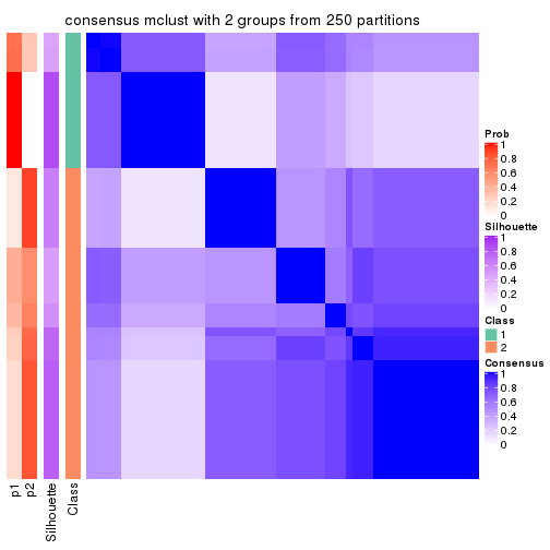
consensus_heatmap(res, k = 3)
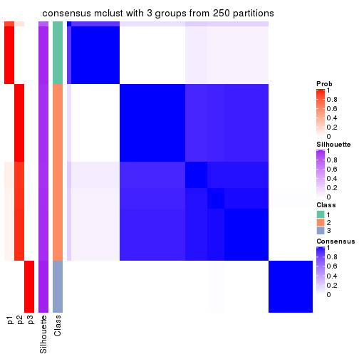
consensus_heatmap(res, k = 4)
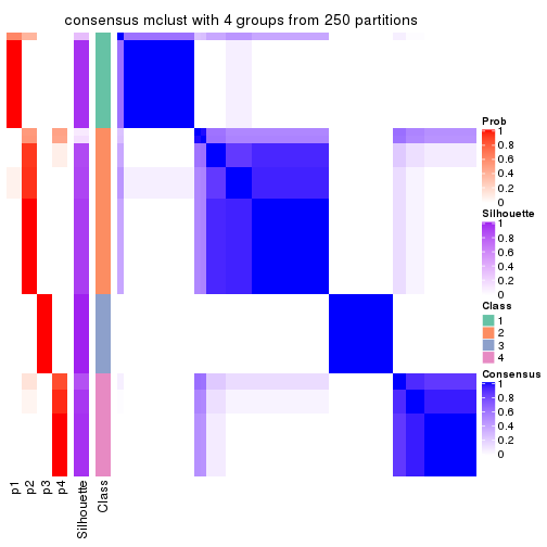
consensus_heatmap(res, k = 5)
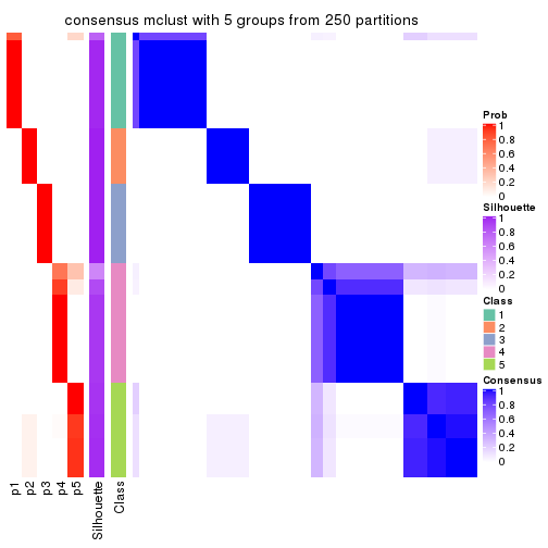
consensus_heatmap(res, k = 6)
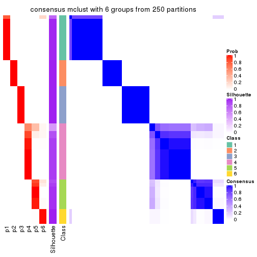
Heatmaps for the membership of samples in all partitions to see how consistent they are:
membership_heatmap(res, k = 2)
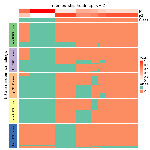
membership_heatmap(res, k = 3)
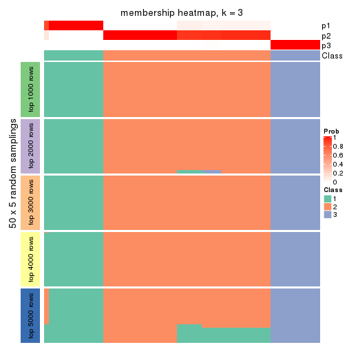
membership_heatmap(res, k = 4)
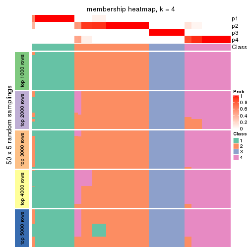
membership_heatmap(res, k = 5)
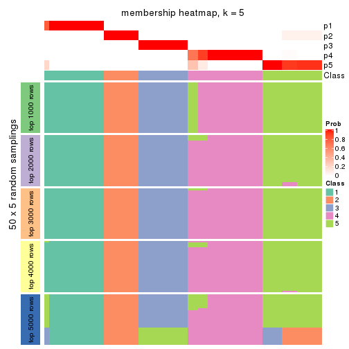
membership_heatmap(res, k = 6)
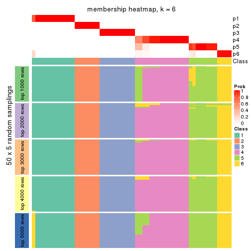
As soon as we have had the classes for columns, we can look for signatures which are significantly different between classes which can be candidate marks for certain classes. Following are the heatmaps for signatures.
Signature heatmaps where rows are scaled:
get_signatures(res, k = 2)
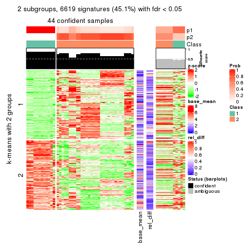
get_signatures(res, k = 3)
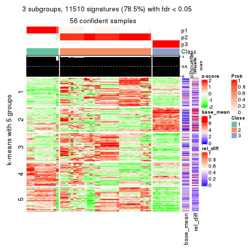
get_signatures(res, k = 4)
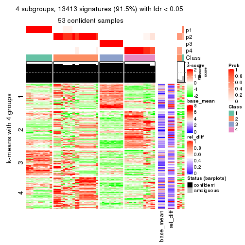
get_signatures(res, k = 5)
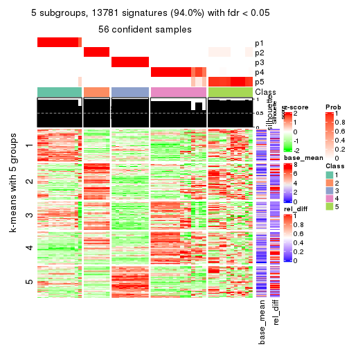
get_signatures(res, k = 6)
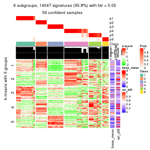
Signature heatmaps where rows are not scaled:
get_signatures(res, k = 2, scale_rows = FALSE)
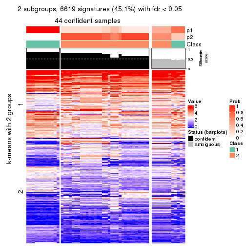
get_signatures(res, k = 3, scale_rows = FALSE)
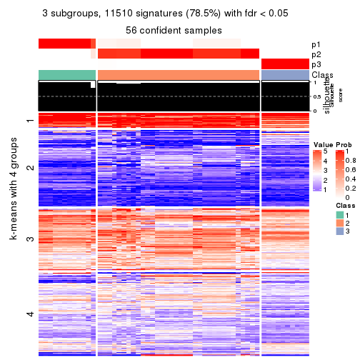
get_signatures(res, k = 4, scale_rows = FALSE)
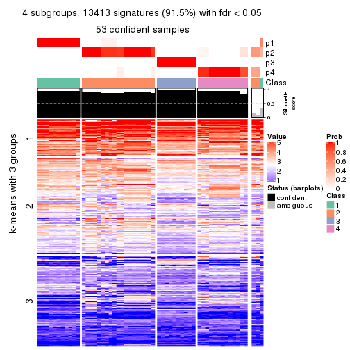
get_signatures(res, k = 5, scale_rows = FALSE)
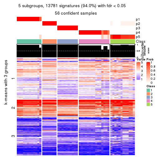
get_signatures(res, k = 6, scale_rows = FALSE)
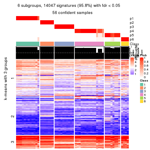
Compare the overlap of signatures from different k:
compare_signatures(res)
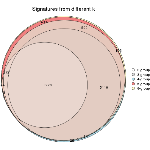
get_signature() returns a data frame invisibly. TO get the list of signatures, the function
call should be assigned to a variable explicitly. In following code, if plot argument is set
to FALSE, no heatmap is plotted while only the differential analysis is performed.
# code only for demonstration
tb = get_signature(res, k = ..., plot = FALSE)
An example of the output of tb is:
#>   which_row         fdr    mean_1    mean_2 scaled_mean_1 scaled_mean_2 km
#> 1        38 0.042760348  8.373488  9.131774    -0.5533452     0.5164555  1
#> 2        40 0.018707592  7.106213  8.469186    -0.6173731     0.5762149  1
#> 3        55 0.019134737 10.221463 11.207825    -0.6159697     0.5749050  1
#> 4        59 0.006059896  5.921854  7.869574    -0.6899429     0.6439467  1
#> 5        60 0.018055526  8.928898 10.211722    -0.6204761     0.5791110  1
#> 6        98 0.009384629 15.714769 14.887706     0.6635654    -0.6193277  2
...
The columns in tb are:
which_row: row indices corresponding to the input matrix.fdr: FDR for the differential test. mean_x: The mean value in group x.scaled_mean_x: The mean value in group x after rows are scaled.km: Row groups if k-means clustering is applied to rows.UMAP plot which shows how samples are separated.
dimension_reduction(res, k = 2, method = "UMAP")
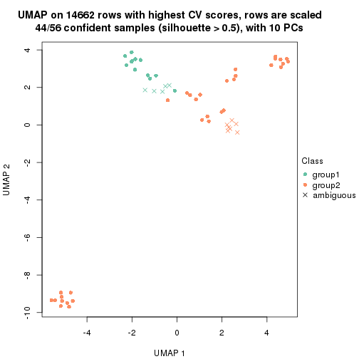
dimension_reduction(res, k = 3, method = "UMAP")
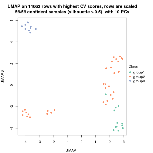
dimension_reduction(res, k = 4, method = "UMAP")
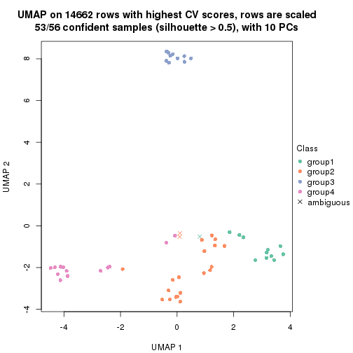
dimension_reduction(res, k = 5, method = "UMAP")
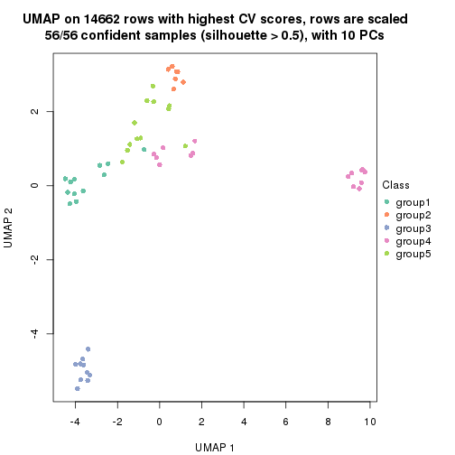
dimension_reduction(res, k = 6, method = "UMAP")

Following heatmap shows how subgroups are split when increasing k:
collect_classes(res)
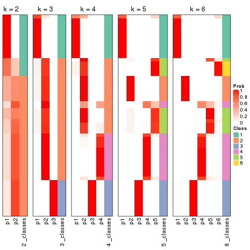
If matrix rows can be associated to genes, consider to use functional_enrichment(res,
...) to perform function enrichment for the signature genes. See this vignette for more detailed explanations.
The object with results only for a single top-value method and a single partition method can be extracted as:
res = res_list["CV", "NMF"]
# you can also extract it by
# res = res_list["CV:NMF"]
A summary of res and all the functions that can be applied to it:
res
#> A 'ConsensusPartition' object with k = 2, 3, 4, 5, 6.
#>   On a matrix with 14662 rows and 56 columns.
#>   Top rows (1000, 2000, 3000, 4000, 5000) are extracted by 'CV' method.
#>   Subgroups are detected by 'NMF' method.
#>   Performed in total 1250 partitions by row resampling.
#>   Best k for subgroups seems to be 6.
#>
#> Following methods can be applied to this 'ConsensusPartition' object:
#>  [1] "cola_report"             "collect_classes"         "collect_plots"
#>  [4] "collect_stats"           "colnames"                "compare_signatures"
#>  [7] "consensus_heatmap"       "dimension_reduction"     "functional_enrichment"
#> [10] "get_anno_col"            "get_anno"                "get_classes"
#> [13] "get_consensus"           "get_matrix"              "get_membership"
#> [16] "get_param"               "get_signatures"          "get_stats"
#> [19] "is_best_k"               "is_stable_k"             "membership_heatmap"
#> [22] "ncol"                    "nrow"                    "plot_ecdf"
#> [25] "rownames"                "select_partition_number" "show"
#> [28] "suggest_best_k"          "test_to_known_factors"
collect_plots() function collects all the plots made from res for all k (number of partitions)
into one single page to provide an easy and fast comparison between different k.
collect_plots(res)
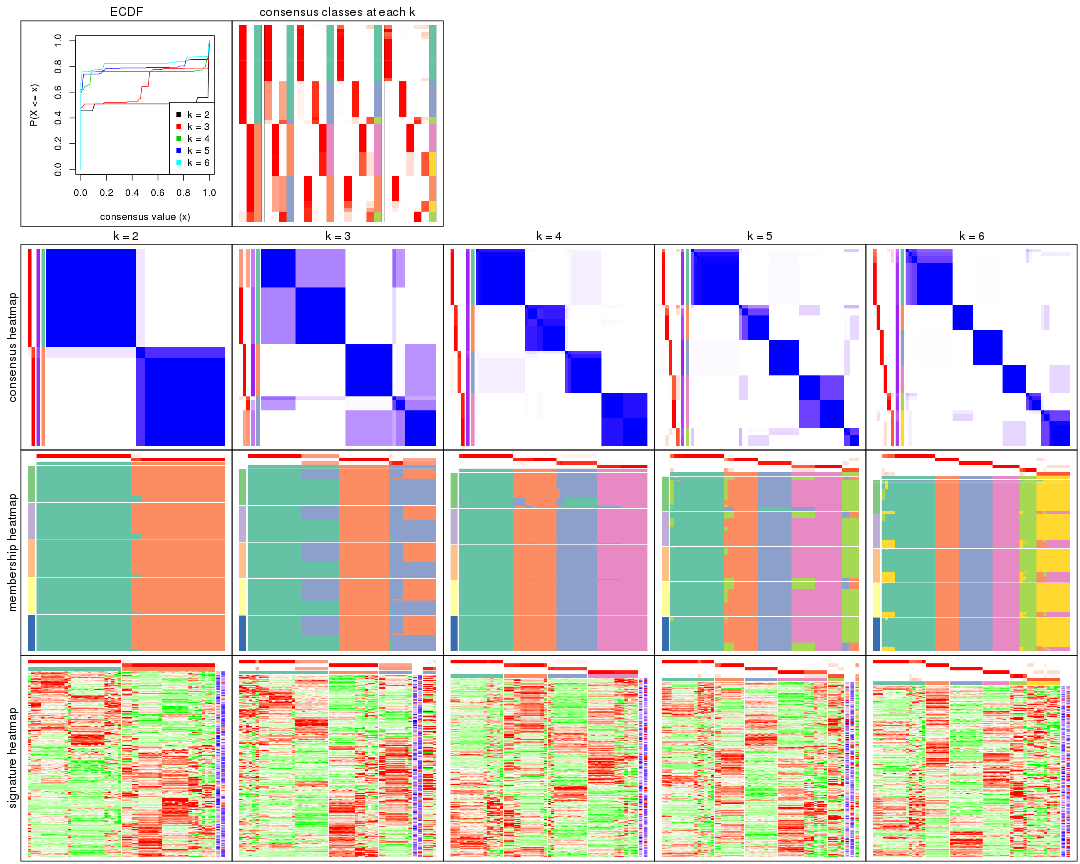
The plots are:
k and the heatmap of
predicted classes for each k.k.k.k.All the plots in panels can be made by individual functions and they are plotted later in this section.
select_partition_number() produces several plots showing different
statistics for choosing “optimized” k. There are following statistics:
k;k, the area increased is defined as \(A_k - A_{k-1}\).The detailed explanations of these statistics can be found in the cola vignette.
Generally speaking, lower PAC score, higher mean silhouette score or higher
concordance corresponds to better partition. Rand index and Jaccard index
measure how similar the current partition is compared to partition with k-1.
If they are too similar, we won't accept k is better than k-1.
select_partition_number(res)
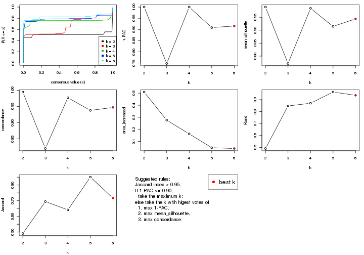
The numeric values for all these statistics can be obtained by get_stats().
get_stats(res)
#>   k 1-PAC mean_silhouette concordance area_increased  Rand Jaccard
#> 2 2 1.000           0.989       0.995         0.5090 0.491   0.491
#> 3 3 0.748           0.771       0.820         0.2766 0.847   0.694
#> 4 4 1.000           0.984       0.977         0.1630 0.870   0.642
#> 5 5 0.908           0.915       0.938         0.0487 0.964   0.851
#> 6 6 0.915           0.944       0.947         0.0420 0.936   0.717
suggest_best_k() suggests the best \(k\) based on these statistics. The rules are as follows:
suggest_best_k(res)
#> [1] 6
#> attr(,"optional")
#> [1] 2 4 5
There is also optional best \(k\) = 2 4 5 that is worth to check.
Following shows the table of the partitions (You need to click the show/hide
code output link to see it). The membership matrix (columns with name p*)
is inferred by
clue::cl_consensus()
function with the SE method. Basically the value in the membership matrix
represents the probability to belong to a certain group. The finall class
label for an item is determined with the group with highest probability it
belongs to.
In get_classes() function, the entropy is calculated from the membership
matrix and the silhouette score is calculated from the consensus matrix.
cbind(get_classes(res, k = 2), get_membership(res, k = 2))
#>           class entropy silhouette    p1    p2
#> SRR073723     1   0.000      1.000 1.000 0.000
#> SRR073724     1   0.000      1.000 1.000 0.000
#> SRR073725     1   0.000      1.000 1.000 0.000
#> SRR073726     2   0.000      0.989 0.000 1.000
#> SRR073727     1   0.000      1.000 1.000 0.000
#> SRR073728     2   0.469      0.897 0.100 0.900
#> SRR073729     2   0.482      0.892 0.104 0.896
#> SRR073730     2   0.469      0.897 0.100 0.900
#> SRR073731     2   0.000      0.989 0.000 1.000
#> SRR073732     2   0.000      0.989 0.000 1.000
#> SRR073733     2   0.000      0.989 0.000 1.000
#> SRR073734     2   0.000      0.989 0.000 1.000
#> SRR073735     2   0.000      0.989 0.000 1.000
#> SRR073736     2   0.000      0.989 0.000 1.000
#> SRR073737     2   0.000      0.989 0.000 1.000
#> SRR073738     1   0.000      1.000 1.000 0.000
#> SRR073739     1   0.000      1.000 1.000 0.000
#> SRR073740     1   0.000      1.000 1.000 0.000
#> SRR073741     1   0.000      1.000 1.000 0.000
#> SRR073742     1   0.000      1.000 1.000 0.000
#> SRR073743     1   0.000      1.000 1.000 0.000
#> SRR073744     1   0.000      1.000 1.000 0.000
#> SRR073745     1   0.000      1.000 1.000 0.000
#> SRR073746     1   0.000      1.000 1.000 0.000
#> SRR073747     1   0.000      1.000 1.000 0.000
#> SRR073748     1   0.000      1.000 1.000 0.000
#> SRR073749     1   0.000      1.000 1.000 0.000
#> SRR073750     1   0.000      1.000 1.000 0.000
#> SRR073751     1   0.000      1.000 1.000 0.000
#> SRR073752     2   0.000      0.989 0.000 1.000
#> SRR073753     2   0.000      0.989 0.000 1.000
#> SRR073754     2   0.000      0.989 0.000 1.000
#> SRR073755     2   0.000      0.989 0.000 1.000
#> SRR073756     2   0.000      0.989 0.000 1.000
#> SRR073758     2   0.000      0.989 0.000 1.000
#> SRR073759     2   0.000      0.989 0.000 1.000
#> SRR073760     2   0.000      0.989 0.000 1.000
#> SRR073761     2   0.000      0.989 0.000 1.000
#> SRR073763     2   0.000      0.989 0.000 1.000
#> SRR073764     2   0.000      0.989 0.000 1.000
#> SRR073765     2   0.000      0.989 0.000 1.000
#> SRR073766     2   0.000      0.989 0.000 1.000
#> SRR073767     2   0.000      0.989 0.000 1.000
#> SRR073768     2   0.000      0.989 0.000 1.000
#> SRR073769     1   0.000      1.000 1.000 0.000
#> SRR073770     1   0.000      1.000 1.000 0.000
#> SRR073771     1   0.000      1.000 1.000 0.000
#> SRR073772     1   0.000      1.000 1.000 0.000
#> SRR073773     1   0.000      1.000 1.000 0.000
#> SRR073774     1   0.000      1.000 1.000 0.000
#> SRR073775     1   0.000      1.000 1.000 0.000
#> SRR073776     1   0.000      1.000 1.000 0.000
#> SRR073777     1   0.000      1.000 1.000 0.000
#> SRR073778     1   0.000      1.000 1.000 0.000
#> SRR073779     2   0.000      0.989 0.000 1.000
#> SRR073780     2   0.000      0.989 0.000 1.000
cbind(get_classes(res, k = 3), get_membership(res, k = 3))
#>           class entropy silhouette    p1    p2    p3
#> SRR073723     1  0.6291     0.6634 0.532 0.000 0.468
#> SRR073724     1  0.0000     0.7974 1.000 0.000 0.000
#> SRR073725     1  0.0000     0.7974 1.000 0.000 0.000
#> SRR073726     2  0.0000     0.9995 0.000 1.000 0.000
#> SRR073727     1  0.0000     0.7974 1.000 0.000 0.000
#> SRR073728     3  0.0747     0.4552 0.000 0.016 0.984
#> SRR073729     3  0.1031     0.4654 0.000 0.024 0.976
#> SRR073730     3  0.0892     0.4607 0.000 0.020 0.980
#> SRR073731     3  0.6291     0.6718 0.000 0.468 0.532
#> SRR073732     3  0.6291     0.6718 0.000 0.468 0.532
#> SRR073733     3  0.6291     0.6718 0.000 0.468 0.532
#> SRR073734     3  0.6291     0.6718 0.000 0.468 0.532
#> SRR073735     3  0.6291     0.6718 0.000 0.468 0.532
#> SRR073736     3  0.6291     0.6718 0.000 0.468 0.532
#> SRR073737     3  0.6291     0.6718 0.000 0.468 0.532
#> SRR073738     1  0.0000     0.7974 1.000 0.000 0.000
#> SRR073739     1  0.0000     0.7974 1.000 0.000 0.000
#> SRR073740     1  0.0000     0.7974 1.000 0.000 0.000
#> SRR073741     1  0.0000     0.7974 1.000 0.000 0.000
#> SRR073742     1  0.0000     0.7974 1.000 0.000 0.000
#> SRR073743     1  0.0000     0.7974 1.000 0.000 0.000
#> SRR073744     1  0.0000     0.7974 1.000 0.000 0.000
#> SRR073745     1  0.0000     0.7974 1.000 0.000 0.000
#> SRR073746     1  0.0000     0.7974 1.000 0.000 0.000
#> SRR073747     1  0.0000     0.7974 1.000 0.000 0.000
#> SRR073748     1  0.0000     0.7974 1.000 0.000 0.000
#> SRR073749     1  0.0000     0.7974 1.000 0.000 0.000
#> SRR073750     1  0.0000     0.7974 1.000 0.000 0.000
#> SRR073751     3  0.4178     0.0601 0.172 0.000 0.828
#> SRR073752     3  0.6291     0.6718 0.000 0.468 0.532
#> SRR073753     3  0.6291     0.6718 0.000 0.468 0.532
#> SRR073754     2  0.0237     0.9935 0.000 0.996 0.004
#> SRR073755     2  0.0000     0.9995 0.000 1.000 0.000
#> SRR073756     2  0.0000     0.9995 0.000 1.000 0.000
#> SRR073758     2  0.0000     0.9995 0.000 1.000 0.000
#> SRR073759     3  0.6291     0.6718 0.000 0.468 0.532
#> SRR073760     2  0.0000     0.9995 0.000 1.000 0.000
#> SRR073761     2  0.0000     0.9995 0.000 1.000 0.000
#> SRR073763     2  0.0000     0.9995 0.000 1.000 0.000
#> SRR073764     2  0.0000     0.9995 0.000 1.000 0.000
#> SRR073765     2  0.0000     0.9995 0.000 1.000 0.000
#> SRR073766     2  0.0000     0.9995 0.000 1.000 0.000
#> SRR073767     2  0.0000     0.9995 0.000 1.000 0.000
#> SRR073768     2  0.0000     0.9995 0.000 1.000 0.000
#> SRR073769     1  0.6291     0.6634 0.532 0.000 0.468
#> SRR073770     1  0.6291     0.6634 0.532 0.000 0.468
#> SRR073771     1  0.6291     0.6634 0.532 0.000 0.468
#> SRR073772     1  0.6291     0.6634 0.532 0.000 0.468
#> SRR073773     1  0.6291     0.6634 0.532 0.000 0.468
#> SRR073774     1  0.6291     0.6634 0.532 0.000 0.468
#> SRR073775     1  0.6291     0.6634 0.532 0.000 0.468
#> SRR073776     1  0.6291     0.6634 0.532 0.000 0.468
#> SRR073777     1  0.6291     0.6634 0.532 0.000 0.468
#> SRR073778     1  0.6291     0.6634 0.532 0.000 0.468
#> SRR073779     2  0.0000     0.9995 0.000 1.000 0.000
#> SRR073780     2  0.0000     0.9995 0.000 1.000 0.000
cbind(get_classes(res, k = 4), get_membership(res, k = 4))
#>           class entropy silhouette    p1    p2    p3    p4
#> SRR073723     3  0.0817      0.943 0.024 0.000 0.976 0.000
#> SRR073724     1  0.0921      0.968 0.972 0.000 0.028 0.000
#> SRR073725     1  0.0000      0.998 1.000 0.000 0.000 0.000
#> SRR073726     4  0.0817      0.988 0.000 0.000 0.024 0.976
#> SRR073727     1  0.0000      0.998 1.000 0.000 0.000 0.000
#> SRR073728     2  0.1389      0.969 0.000 0.952 0.048 0.000
#> SRR073729     2  0.1389      0.969 0.000 0.952 0.048 0.000
#> SRR073730     2  0.1389      0.969 0.000 0.952 0.048 0.000
#> SRR073731     2  0.0000      0.984 0.000 1.000 0.000 0.000
#> SRR073732     2  0.0000      0.984 0.000 1.000 0.000 0.000
#> SRR073733     2  0.0000      0.984 0.000 1.000 0.000 0.000
#> SRR073734     2  0.0000      0.984 0.000 1.000 0.000 0.000
#> SRR073735     2  0.0000      0.984 0.000 1.000 0.000 0.000
#> SRR073736     2  0.0000      0.984 0.000 1.000 0.000 0.000
#> SRR073737     2  0.0000      0.984 0.000 1.000 0.000 0.000
#> SRR073738     1  0.0188      0.993 0.996 0.000 0.000 0.004
#> SRR073739     1  0.0000      0.998 1.000 0.000 0.000 0.000
#> SRR073740     1  0.0000      0.998 1.000 0.000 0.000 0.000
#> SRR073741     1  0.0000      0.998 1.000 0.000 0.000 0.000
#> SRR073742     1  0.0000      0.998 1.000 0.000 0.000 0.000
#> SRR073743     1  0.0000      0.998 1.000 0.000 0.000 0.000
#> SRR073744     1  0.0000      0.998 1.000 0.000 0.000 0.000
#> SRR073745     1  0.0000      0.998 1.000 0.000 0.000 0.000
#> SRR073746     1  0.0000      0.998 1.000 0.000 0.000 0.000
#> SRR073747     1  0.0000      0.998 1.000 0.000 0.000 0.000
#> SRR073748     1  0.0000      0.998 1.000 0.000 0.000 0.000
#> SRR073749     1  0.0000      0.998 1.000 0.000 0.000 0.000
#> SRR073750     1  0.0000      0.998 1.000 0.000 0.000 0.000
#> SRR073751     3  0.2053      0.877 0.004 0.072 0.924 0.000
#> SRR073752     2  0.0817      0.974 0.000 0.976 0.024 0.000
#> SRR073753     2  0.0817      0.974 0.000 0.976 0.024 0.000
#> SRR073754     4  0.1004      0.986 0.000 0.004 0.024 0.972
#> SRR073755     4  0.0817      0.988 0.000 0.000 0.024 0.976
#> SRR073756     4  0.0817      0.988 0.000 0.000 0.024 0.976
#> SRR073758     4  0.0817      0.988 0.000 0.000 0.024 0.976
#> SRR073759     2  0.1637      0.966 0.000 0.940 0.060 0.000
#> SRR073760     4  0.0000      0.990 0.000 0.000 0.000 1.000
#> SRR073761     4  0.0000      0.990 0.000 0.000 0.000 1.000
#> SRR073763     4  0.0000      0.990 0.000 0.000 0.000 1.000
#> SRR073764     4  0.0000      0.990 0.000 0.000 0.000 1.000
#> SRR073765     4  0.0000      0.990 0.000 0.000 0.000 1.000
#> SRR073766     4  0.0000      0.990 0.000 0.000 0.000 1.000
#> SRR073767     4  0.0000      0.990 0.000 0.000 0.000 1.000
#> SRR073768     4  0.0000      0.990 0.000 0.000 0.000 1.000
#> SRR073769     3  0.1867      0.985 0.072 0.000 0.928 0.000
#> SRR073770     3  0.1867      0.985 0.072 0.000 0.928 0.000
#> SRR073771     3  0.1867      0.985 0.072 0.000 0.928 0.000
#> SRR073772     3  0.1867      0.985 0.072 0.000 0.928 0.000
#> SRR073773     3  0.1867      0.985 0.072 0.000 0.928 0.000
#> SRR073774     3  0.1867      0.985 0.072 0.000 0.928 0.000
#> SRR073775     3  0.1867      0.985 0.072 0.000 0.928 0.000
#> SRR073776     3  0.1867      0.985 0.072 0.000 0.928 0.000
#> SRR073777     3  0.1867      0.985 0.072 0.000 0.928 0.000
#> SRR073778     3  0.1867      0.985 0.072 0.000 0.928 0.000
#> SRR073779     4  0.0817      0.988 0.000 0.000 0.024 0.976
#> SRR073780     4  0.0817      0.988 0.000 0.000 0.024 0.976
cbind(get_classes(res, k = 5), get_membership(res, k = 5))
#>           class entropy silhouette    p1    p2    p3    p4    p5
#> SRR073723     5  0.2813      0.812 0.000 0.000 0.168 0.000 0.832
#> SRR073724     1  0.3395      0.687 0.764 0.000 0.000 0.000 0.236
#> SRR073725     1  0.0000      0.982 1.000 0.000 0.000 0.000 0.000
#> SRR073726     4  0.3399      0.889 0.000 0.000 0.020 0.812 0.168
#> SRR073727     1  0.0510      0.967 0.984 0.000 0.000 0.000 0.016
#> SRR073728     5  0.2813      0.878 0.000 0.168 0.000 0.000 0.832
#> SRR073729     5  0.2813      0.878 0.000 0.168 0.000 0.000 0.832
#> SRR073730     5  0.2813      0.878 0.000 0.168 0.000 0.000 0.832
#> SRR073731     2  0.0000      0.891 0.000 1.000 0.000 0.000 0.000
#> SRR073732     2  0.0000      0.891 0.000 1.000 0.000 0.000 0.000
#> SRR073733     2  0.0000      0.891 0.000 1.000 0.000 0.000 0.000
#> SRR073734     2  0.0000      0.891 0.000 1.000 0.000 0.000 0.000
#> SRR073735     2  0.0000      0.891 0.000 1.000 0.000 0.000 0.000
#> SRR073736     2  0.0000      0.891 0.000 1.000 0.000 0.000 0.000
#> SRR073737     2  0.0000      0.891 0.000 1.000 0.000 0.000 0.000
#> SRR073738     1  0.0162      0.979 0.996 0.000 0.000 0.000 0.004
#> SRR073739     1  0.0000      0.982 1.000 0.000 0.000 0.000 0.000
#> SRR073740     1  0.0000      0.982 1.000 0.000 0.000 0.000 0.000
#> SRR073741     1  0.0000      0.982 1.000 0.000 0.000 0.000 0.000
#> SRR073742     1  0.0000      0.982 1.000 0.000 0.000 0.000 0.000
#> SRR073743     1  0.0000      0.982 1.000 0.000 0.000 0.000 0.000
#> SRR073744     1  0.0000      0.982 1.000 0.000 0.000 0.000 0.000
#> SRR073745     1  0.0000      0.982 1.000 0.000 0.000 0.000 0.000
#> SRR073746     1  0.0000      0.982 1.000 0.000 0.000 0.000 0.000
#> SRR073747     1  0.0000      0.982 1.000 0.000 0.000 0.000 0.000
#> SRR073748     1  0.0000      0.982 1.000 0.000 0.000 0.000 0.000
#> SRR073749     1  0.0000      0.982 1.000 0.000 0.000 0.000 0.000
#> SRR073750     1  0.0290      0.975 0.992 0.000 0.008 0.000 0.000
#> SRR073751     5  0.3194      0.835 0.000 0.020 0.148 0.000 0.832
#> SRR073752     2  0.3359      0.763 0.000 0.816 0.020 0.000 0.164
#> SRR073753     2  0.3359      0.763 0.000 0.816 0.020 0.000 0.164
#> SRR073754     4  0.3399      0.889 0.000 0.000 0.020 0.812 0.168
#> SRR073755     4  0.3399      0.889 0.000 0.000 0.020 0.812 0.168
#> SRR073756     4  0.3399      0.889 0.000 0.000 0.020 0.812 0.168
#> SRR073758     4  0.3399      0.889 0.000 0.000 0.020 0.812 0.168
#> SRR073759     2  0.4826      0.329 0.000 0.508 0.020 0.000 0.472
#> SRR073760     4  0.0000      0.904 0.000 0.000 0.000 1.000 0.000
#> SRR073761     4  0.0000      0.904 0.000 0.000 0.000 1.000 0.000
#> SRR073763     4  0.0000      0.904 0.000 0.000 0.000 1.000 0.000
#> SRR073764     4  0.0000      0.904 0.000 0.000 0.000 1.000 0.000
#> SRR073765     4  0.0000      0.904 0.000 0.000 0.000 1.000 0.000
#> SRR073766     4  0.0000      0.904 0.000 0.000 0.000 1.000 0.000
#> SRR073767     4  0.0000      0.904 0.000 0.000 0.000 1.000 0.000
#> SRR073768     4  0.0000      0.904 0.000 0.000 0.000 1.000 0.000
#> SRR073769     3  0.0609      1.000 0.020 0.000 0.980 0.000 0.000
#> SRR073770     3  0.0609      1.000 0.020 0.000 0.980 0.000 0.000
#> SRR073771     3  0.0609      1.000 0.020 0.000 0.980 0.000 0.000
#> SRR073772     3  0.0609      1.000 0.020 0.000 0.980 0.000 0.000
#> SRR073773     3  0.0609      1.000 0.020 0.000 0.980 0.000 0.000
#> SRR073774     3  0.0609      1.000 0.020 0.000 0.980 0.000 0.000
#> SRR073775     3  0.0609      1.000 0.020 0.000 0.980 0.000 0.000
#> SRR073776     3  0.0609      1.000 0.020 0.000 0.980 0.000 0.000
#> SRR073777     3  0.0609      1.000 0.020 0.000 0.980 0.000 0.000
#> SRR073778     3  0.0609      1.000 0.020 0.000 0.980 0.000 0.000
#> SRR073779     4  0.3399      0.889 0.000 0.000 0.020 0.812 0.168
#> SRR073780     4  0.3399      0.889 0.000 0.000 0.020 0.812 0.168
cbind(get_classes(res, k = 6), get_membership(res, k = 6))
#>           class entropy silhouette    p1    p2    p3    p4    p5    p6
#> SRR073723     5  0.2738      0.853 0.000 0.000 0.004 0.000 0.820 0.176
#> SRR073724     1  0.4757      0.678 0.688 0.000 0.004 0.000 0.132 0.176
#> SRR073725     1  0.0000      0.943 1.000 0.000 0.000 0.000 0.000 0.000
#> SRR073726     6  0.2597      0.918 0.000 0.000 0.000 0.176 0.000 0.824
#> SRR073727     1  0.3265      0.766 0.748 0.000 0.004 0.000 0.000 0.248
#> SRR073728     5  0.0000      0.950 0.000 0.000 0.000 0.000 1.000 0.000
#> SRR073729     5  0.0000      0.950 0.000 0.000 0.000 0.000 1.000 0.000
#> SRR073730     5  0.0000      0.950 0.000 0.000 0.000 0.000 1.000 0.000
#> SRR073731     2  0.0000      1.000 0.000 1.000 0.000 0.000 0.000 0.000
#> SRR073732     2  0.0000      1.000 0.000 1.000 0.000 0.000 0.000 0.000
#> SRR073733     2  0.0000      1.000 0.000 1.000 0.000 0.000 0.000 0.000
#> SRR073734     2  0.0000      1.000 0.000 1.000 0.000 0.000 0.000 0.000
#> SRR073735     2  0.0000      1.000 0.000 1.000 0.000 0.000 0.000 0.000
#> SRR073736     2  0.0000      1.000 0.000 1.000 0.000 0.000 0.000 0.000
#> SRR073737     2  0.0000      1.000 0.000 1.000 0.000 0.000 0.000 0.000
#> SRR073738     1  0.2738      0.831 0.820 0.000 0.004 0.000 0.000 0.176
#> SRR073739     1  0.0000      0.943 1.000 0.000 0.000 0.000 0.000 0.000
#> SRR073740     1  0.0000      0.943 1.000 0.000 0.000 0.000 0.000 0.000
#> SRR073741     1  0.0000      0.943 1.000 0.000 0.000 0.000 0.000 0.000
#> SRR073742     1  0.0000      0.943 1.000 0.000 0.000 0.000 0.000 0.000
#> SRR073743     1  0.0000      0.943 1.000 0.000 0.000 0.000 0.000 0.000
#> SRR073744     1  0.0000      0.943 1.000 0.000 0.000 0.000 0.000 0.000
#> SRR073745     1  0.0000      0.943 1.000 0.000 0.000 0.000 0.000 0.000
#> SRR073746     1  0.0000      0.943 1.000 0.000 0.000 0.000 0.000 0.000
#> SRR073747     1  0.0000      0.943 1.000 0.000 0.000 0.000 0.000 0.000
#> SRR073748     1  0.0000      0.943 1.000 0.000 0.000 0.000 0.000 0.000
#> SRR073749     1  0.0000      0.943 1.000 0.000 0.000 0.000 0.000 0.000
#> SRR073750     1  0.2597      0.834 0.824 0.000 0.000 0.000 0.000 0.176
#> SRR073751     5  0.1141      0.937 0.000 0.000 0.000 0.000 0.948 0.052
#> SRR073752     6  0.2772      0.786 0.000 0.180 0.004 0.000 0.000 0.816
#> SRR073753     6  0.2772      0.786 0.000 0.180 0.004 0.000 0.000 0.816
#> SRR073754     6  0.2527      0.915 0.000 0.000 0.000 0.168 0.000 0.832
#> SRR073755     6  0.2597      0.918 0.000 0.000 0.000 0.176 0.000 0.824
#> SRR073756     6  0.2597      0.918 0.000 0.000 0.000 0.176 0.000 0.824
#> SRR073758     6  0.2597      0.918 0.000 0.000 0.000 0.176 0.000 0.824
#> SRR073759     6  0.3277      0.800 0.000 0.092 0.000 0.000 0.084 0.824
#> SRR073760     4  0.0000      1.000 0.000 0.000 0.000 1.000 0.000 0.000
#> SRR073761     4  0.0000      1.000 0.000 0.000 0.000 1.000 0.000 0.000
#> SRR073763     4  0.0000      1.000 0.000 0.000 0.000 1.000 0.000 0.000
#> SRR073764     4  0.0000      1.000 0.000 0.000 0.000 1.000 0.000 0.000
#> SRR073765     4  0.0000      1.000 0.000 0.000 0.000 1.000 0.000 0.000
#> SRR073766     4  0.0000      1.000 0.000 0.000 0.000 1.000 0.000 0.000
#> SRR073767     4  0.0000      1.000 0.000 0.000 0.000 1.000 0.000 0.000
#> SRR073768     4  0.0000      1.000 0.000 0.000 0.000 1.000 0.000 0.000
#> SRR073769     3  0.0146      1.000 0.004 0.000 0.996 0.000 0.000 0.000
#> SRR073770     3  0.0146      1.000 0.004 0.000 0.996 0.000 0.000 0.000
#> SRR073771     3  0.0146      1.000 0.004 0.000 0.996 0.000 0.000 0.000
#> SRR073772     3  0.0146      1.000 0.004 0.000 0.996 0.000 0.000 0.000
#> SRR073773     3  0.0146      1.000 0.004 0.000 0.996 0.000 0.000 0.000
#> SRR073774     3  0.0146      1.000 0.004 0.000 0.996 0.000 0.000 0.000
#> SRR073775     3  0.0146      1.000 0.004 0.000 0.996 0.000 0.000 0.000
#> SRR073776     3  0.0146      1.000 0.004 0.000 0.996 0.000 0.000 0.000
#> SRR073777     3  0.0146      1.000 0.004 0.000 0.996 0.000 0.000 0.000
#> SRR073778     3  0.0146      1.000 0.004 0.000 0.996 0.000 0.000 0.000
#> SRR073779     6  0.2597      0.918 0.000 0.000 0.000 0.176 0.000 0.824
#> SRR073780     6  0.2597      0.918 0.000 0.000 0.000 0.176 0.000 0.824
Heatmaps for the consensus matrix. It visualizes the probability of two samples to be in a same group.
consensus_heatmap(res, k = 2)
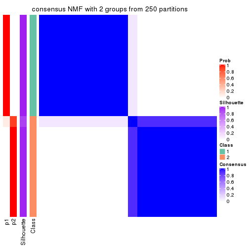
consensus_heatmap(res, k = 3)
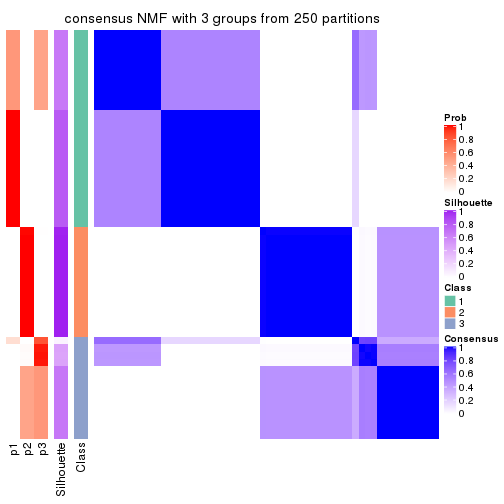
consensus_heatmap(res, k = 4)

consensus_heatmap(res, k = 5)
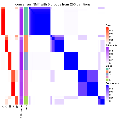
consensus_heatmap(res, k = 6)
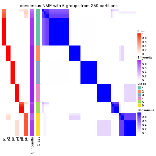
Heatmaps for the membership of samples in all partitions to see how consistent they are:
membership_heatmap(res, k = 2)

membership_heatmap(res, k = 3)
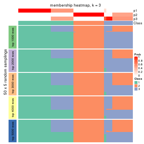
membership_heatmap(res, k = 4)
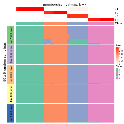
membership_heatmap(res, k = 5)
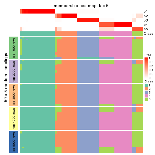
membership_heatmap(res, k = 6)
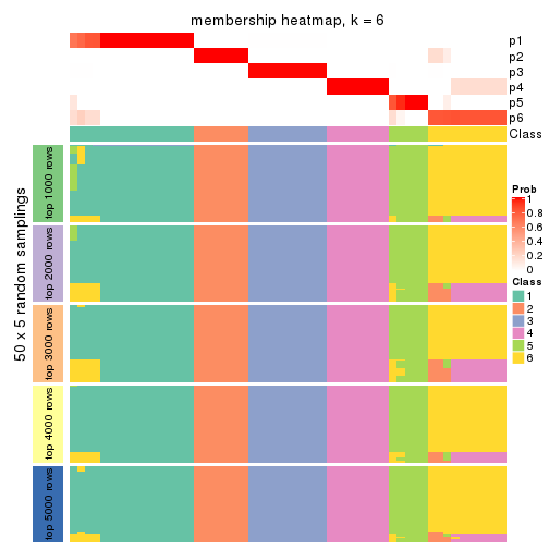
As soon as we have had the classes for columns, we can look for signatures which are significantly different between classes which can be candidate marks for certain classes. Following are the heatmaps for signatures.
Signature heatmaps where rows are scaled:
get_signatures(res, k = 2)

get_signatures(res, k = 3)
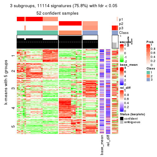
get_signatures(res, k = 4)

get_signatures(res, k = 5)
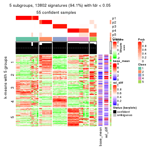
get_signatures(res, k = 6)
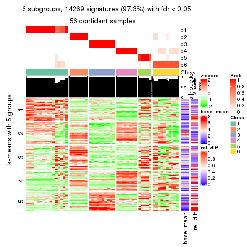
Signature heatmaps where rows are not scaled:
get_signatures(res, k = 2, scale_rows = FALSE)

get_signatures(res, k = 3, scale_rows = FALSE)
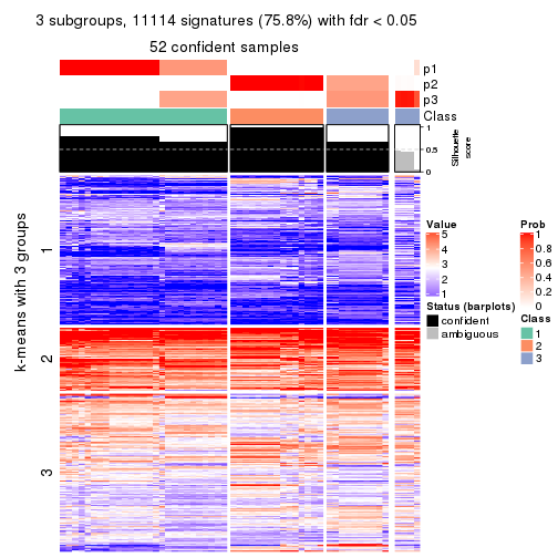
get_signatures(res, k = 4, scale_rows = FALSE)

get_signatures(res, k = 5, scale_rows = FALSE)
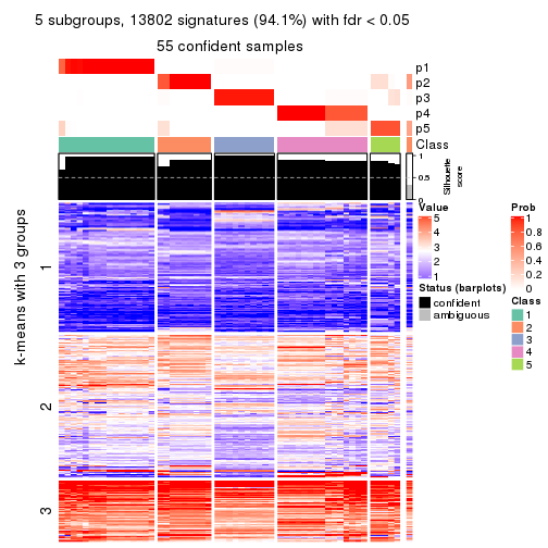
get_signatures(res, k = 6, scale_rows = FALSE)
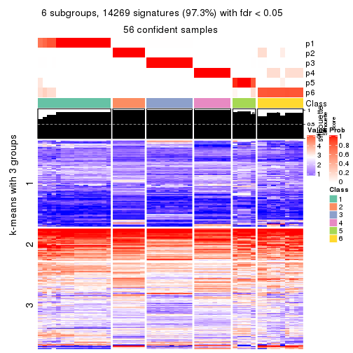
Compare the overlap of signatures from different k:
compare_signatures(res)
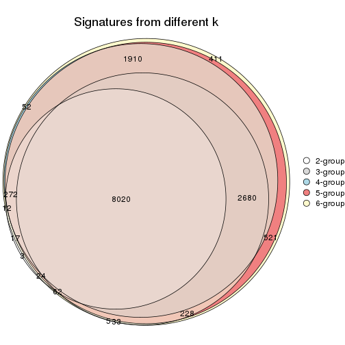
get_signature() returns a data frame invisibly. TO get the list of signatures, the function
call should be assigned to a variable explicitly. In following code, if plot argument is set
to FALSE, no heatmap is plotted while only the differential analysis is performed.
# code only for demonstration
tb = get_signature(res, k = ..., plot = FALSE)
An example of the output of tb is:
#>   which_row         fdr    mean_1    mean_2 scaled_mean_1 scaled_mean_2 km
#> 1        38 0.042760348  8.373488  9.131774    -0.5533452     0.5164555  1
#> 2        40 0.018707592  7.106213  8.469186    -0.6173731     0.5762149  1
#> 3        55 0.019134737 10.221463 11.207825    -0.6159697     0.5749050  1
#> 4        59 0.006059896  5.921854  7.869574    -0.6899429     0.6439467  1
#> 5        60 0.018055526  8.928898 10.211722    -0.6204761     0.5791110  1
#> 6        98 0.009384629 15.714769 14.887706     0.6635654    -0.6193277  2
...
The columns in tb are:
which_row: row indices corresponding to the input matrix.fdr: FDR for the differential test. mean_x: The mean value in group x.scaled_mean_x: The mean value in group x after rows are scaled.km: Row groups if k-means clustering is applied to rows.UMAP plot which shows how samples are separated.
dimension_reduction(res, k = 2, method = "UMAP")

dimension_reduction(res, k = 3, method = "UMAP")
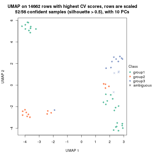
dimension_reduction(res, k = 4, method = "UMAP")

dimension_reduction(res, k = 5, method = "UMAP")

dimension_reduction(res, k = 6, method = "UMAP")
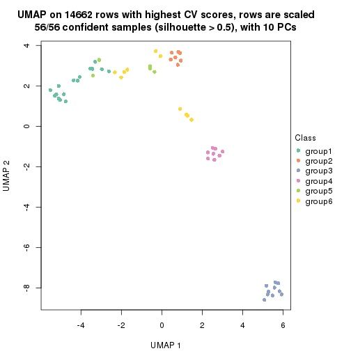
Following heatmap shows how subgroups are split when increasing k:
collect_classes(res)
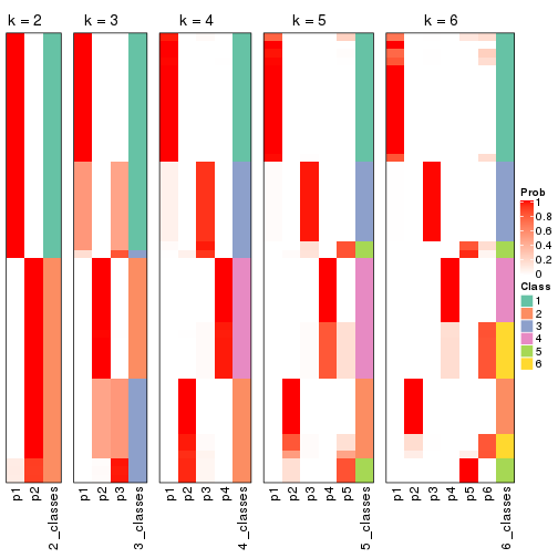
If matrix rows can be associated to genes, consider to use functional_enrichment(res,
...) to perform function enrichment for the signature genes. See this vignette for more detailed explanations.
The object with results only for a single top-value method and a single partition method can be extracted as:
res = res_list["MAD", "hclust"]
# you can also extract it by
# res = res_list["MAD:hclust"]
A summary of res and all the functions that can be applied to it:
res
#> A 'ConsensusPartition' object with k = 2, 3, 4, 5, 6.
#>   On a matrix with 14662 rows and 56 columns.
#>   Top rows (1000, 2000, 3000, 4000, 5000) are extracted by 'MAD' method.
#>   Subgroups are detected by 'hclust' method.
#>   Performed in total 1250 partitions by row resampling.
#>   Best k for subgroups seems to be 3.
#>
#> Following methods can be applied to this 'ConsensusPartition' object:
#>  [1] "cola_report"             "collect_classes"         "collect_plots"
#>  [4] "collect_stats"           "colnames"                "compare_signatures"
#>  [7] "consensus_heatmap"       "dimension_reduction"     "functional_enrichment"
#> [10] "get_anno_col"            "get_anno"                "get_classes"
#> [13] "get_consensus"           "get_matrix"              "get_membership"
#> [16] "get_param"               "get_signatures"          "get_stats"
#> [19] "is_best_k"               "is_stable_k"             "membership_heatmap"
#> [22] "ncol"                    "nrow"                    "plot_ecdf"
#> [25] "rownames"                "select_partition_number" "show"
#> [28] "suggest_best_k"          "test_to_known_factors"
collect_plots() function collects all the plots made from res for all k (number of partitions)
into one single page to provide an easy and fast comparison between different k.
collect_plots(res)
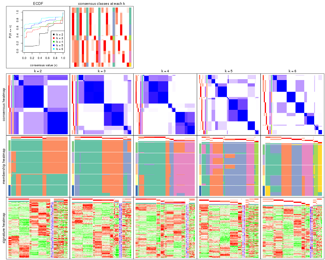
The plots are:
k and the heatmap of
predicted classes for each k.k.k.k.All the plots in panels can be made by individual functions and they are plotted later in this section.
select_partition_number() produces several plots showing different
statistics for choosing “optimized” k. There are following statistics:
k;k, the area increased is defined as \(A_k - A_{k-1}\).The detailed explanations of these statistics can be found in the cola vignette.
Generally speaking, lower PAC score, higher mean silhouette score or higher
concordance corresponds to better partition. Rand index and Jaccard index
measure how similar the current partition is compared to partition with k-1.
If they are too similar, we won't accept k is better than k-1.
select_partition_number(res)
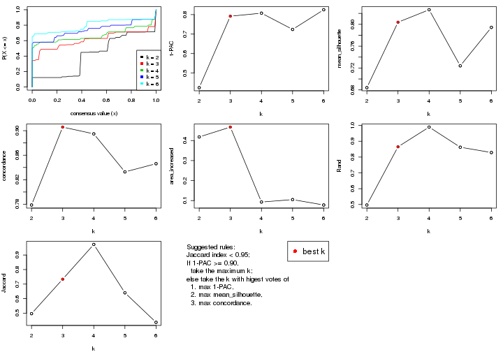
The numeric values for all these statistics can be obtained by get_stats().
get_stats(res)
#>   k 1-PAC mean_silhouette concordance area_increased  Rand Jaccard
#> 2 2 0.425           0.684       0.779         0.4181 0.497   0.497
#> 3 3 0.792           0.804       0.906         0.4673 0.865   0.734
#> 4 4 0.807           0.827       0.895         0.0928 0.990   0.973
#> 5 5 0.724           0.724       0.833         0.1049 0.862   0.640
#> 6 6 0.825           0.794       0.846         0.0780 0.829   0.437
suggest_best_k() suggests the best \(k\) based on these statistics. The rules are as follows:
suggest_best_k(res)
#> [1] 3
Following shows the table of the partitions (You need to click the show/hide
code output link to see it). The membership matrix (columns with name p*)
is inferred by
clue::cl_consensus()
function with the SE method. Basically the value in the membership matrix
represents the probability to belong to a certain group. The finall class
label for an item is determined with the group with highest probability it
belongs to.
In get_classes() function, the entropy is calculated from the membership
matrix and the silhouette score is calculated from the consensus matrix.
cbind(get_classes(res, k = 2), get_membership(res, k = 2))
#>           class entropy silhouette    p1    p2
#> SRR073723     1   0.913    -0.0461 0.672 0.328
#> SRR073724     1   0.963     0.4773 0.612 0.388
#> SRR073725     1   0.963     0.4773 0.612 0.388
#> SRR073726     2   0.000     0.4680 0.000 1.000
#> SRR073727     1   0.963     0.4773 0.612 0.388
#> SRR073728     1   0.955    -0.2442 0.624 0.376
#> SRR073729     1   0.955    -0.2442 0.624 0.376
#> SRR073730     1   0.955    -0.2442 0.624 0.376
#> SRR073731     2   0.963     0.8831 0.388 0.612
#> SRR073732     2   0.963     0.8831 0.388 0.612
#> SRR073733     2   0.963     0.8831 0.388 0.612
#> SRR073734     2   0.963     0.8831 0.388 0.612
#> SRR073735     2   0.963     0.8831 0.388 0.612
#> SRR073736     2   0.963     0.8831 0.388 0.612
#> SRR073737     2   0.963     0.8831 0.388 0.612
#> SRR073738     1   0.963     0.4773 0.612 0.388
#> SRR073739     1   0.000     0.7910 1.000 0.000
#> SRR073740     1   0.000     0.7910 1.000 0.000
#> SRR073741     1   0.000     0.7910 1.000 0.000
#> SRR073742     1   0.000     0.7910 1.000 0.000
#> SRR073743     1   0.000     0.7910 1.000 0.000
#> SRR073744     1   0.000     0.7910 1.000 0.000
#> SRR073745     1   0.000     0.7910 1.000 0.000
#> SRR073746     1   0.000     0.7910 1.000 0.000
#> SRR073747     1   0.000     0.7910 1.000 0.000
#> SRR073748     1   0.000     0.7910 1.000 0.000
#> SRR073749     1   0.000     0.7910 1.000 0.000
#> SRR073750     1   0.963     0.4773 0.612 0.388
#> SRR073751     1   0.995    -0.3268 0.540 0.460
#> SRR073752     2   0.963     0.8831 0.388 0.612
#> SRR073753     2   0.963     0.8831 0.388 0.612
#> SRR073754     2   0.000     0.4680 0.000 1.000
#> SRR073755     2   0.963     0.8831 0.388 0.612
#> SRR073756     2   0.963     0.8831 0.388 0.612
#> SRR073758     2   0.963     0.8831 0.388 0.612
#> SRR073759     2   0.963     0.8831 0.388 0.612
#> SRR073760     2   0.963     0.8831 0.388 0.612
#> SRR073761     2   0.963     0.8831 0.388 0.612
#> SRR073763     2   0.963     0.8831 0.388 0.612
#> SRR073764     2   0.963     0.8831 0.388 0.612
#> SRR073765     2   0.963     0.8831 0.388 0.612
#> SRR073766     2   0.963     0.8831 0.388 0.612
#> SRR073767     2   0.963     0.8831 0.388 0.612
#> SRR073768     2   0.963     0.8831 0.388 0.612
#> SRR073769     1   0.000     0.7910 1.000 0.000
#> SRR073770     1   0.000     0.7910 1.000 0.000
#> SRR073771     1   0.000     0.7910 1.000 0.000
#> SRR073772     1   0.000     0.7910 1.000 0.000
#> SRR073773     1   0.000     0.7910 1.000 0.000
#> SRR073774     1   0.000     0.7910 1.000 0.000
#> SRR073775     1   0.000     0.7910 1.000 0.000
#> SRR073776     1   0.000     0.7910 1.000 0.000
#> SRR073777     1   0.000     0.7910 1.000 0.000
#> SRR073778     1   0.000     0.7910 1.000 0.000
#> SRR073779     2   0.000     0.4680 0.000 1.000
#> SRR073780     2   0.000     0.4680 0.000 1.000
cbind(get_classes(res, k = 3), get_membership(res, k = 3))
#>           class entropy silhouette    p1    p2    p3
#> SRR073723     1  0.5785      0.201 0.668 0.000 0.332
#> SRR073724     1  0.6079      0.414 0.612 0.000 0.388
#> SRR073725     1  0.6079      0.414 0.612 0.000 0.388
#> SRR073726     3  0.4654      0.605 0.000 0.208 0.792
#> SRR073727     1  0.6079      0.414 0.612 0.000 0.388
#> SRR073728     3  0.6180      0.462 0.416 0.000 0.584
#> SRR073729     3  0.6180      0.462 0.416 0.000 0.584
#> SRR073730     3  0.6180      0.462 0.416 0.000 0.584
#> SRR073731     2  0.0000      0.963 0.000 1.000 0.000
#> SRR073732     2  0.0000      0.963 0.000 1.000 0.000
#> SRR073733     2  0.0000      0.963 0.000 1.000 0.000
#> SRR073734     2  0.0000      0.963 0.000 1.000 0.000
#> SRR073735     2  0.0000      0.963 0.000 1.000 0.000
#> SRR073736     2  0.0000      0.963 0.000 1.000 0.000
#> SRR073737     2  0.0000      0.963 0.000 1.000 0.000
#> SRR073738     1  0.6079      0.414 0.612 0.000 0.388
#> SRR073739     1  0.0000      0.876 1.000 0.000 0.000
#> SRR073740     1  0.0000      0.876 1.000 0.000 0.000
#> SRR073741     1  0.0000      0.876 1.000 0.000 0.000
#> SRR073742     1  0.0000      0.876 1.000 0.000 0.000
#> SRR073743     1  0.0000      0.876 1.000 0.000 0.000
#> SRR073744     1  0.0000      0.876 1.000 0.000 0.000
#> SRR073745     1  0.0000      0.876 1.000 0.000 0.000
#> SRR073746     1  0.0000      0.876 1.000 0.000 0.000
#> SRR073747     1  0.0000      0.876 1.000 0.000 0.000
#> SRR073748     1  0.0000      0.876 1.000 0.000 0.000
#> SRR073749     1  0.0000      0.876 1.000 0.000 0.000
#> SRR073750     1  0.6079      0.414 0.612 0.000 0.388
#> SRR073751     3  0.5810      0.526 0.336 0.000 0.664
#> SRR073752     2  0.0000      0.963 0.000 1.000 0.000
#> SRR073753     2  0.0000      0.963 0.000 1.000 0.000
#> SRR073754     3  0.4654      0.605 0.000 0.208 0.792
#> SRR073755     2  0.0000      0.963 0.000 1.000 0.000
#> SRR073756     2  0.0000      0.963 0.000 1.000 0.000
#> SRR073758     2  0.0000      0.963 0.000 1.000 0.000
#> SRR073759     2  0.0000      0.963 0.000 1.000 0.000
#> SRR073760     2  0.2550      0.937 0.056 0.932 0.012
#> SRR073761     2  0.2550      0.937 0.056 0.932 0.012
#> SRR073763     2  0.2550      0.937 0.056 0.932 0.012
#> SRR073764     2  0.2550      0.937 0.056 0.932 0.012
#> SRR073765     2  0.2550      0.937 0.056 0.932 0.012
#> SRR073766     2  0.2550      0.937 0.056 0.932 0.012
#> SRR073767     2  0.2550      0.937 0.056 0.932 0.012
#> SRR073768     2  0.2550      0.937 0.056 0.932 0.012
#> SRR073769     1  0.0237      0.876 0.996 0.000 0.004
#> SRR073770     1  0.0237      0.876 0.996 0.000 0.004
#> SRR073771     1  0.0237      0.876 0.996 0.000 0.004
#> SRR073772     1  0.0237      0.876 0.996 0.000 0.004
#> SRR073773     1  0.0237      0.876 0.996 0.000 0.004
#> SRR073774     1  0.0237      0.876 0.996 0.000 0.004
#> SRR073775     1  0.0237      0.876 0.996 0.000 0.004
#> SRR073776     1  0.0237      0.876 0.996 0.000 0.004
#> SRR073777     1  0.0237      0.876 0.996 0.000 0.004
#> SRR073778     1  0.0237      0.876 0.996 0.000 0.004
#> SRR073779     3  0.4654      0.605 0.000 0.208 0.792
#> SRR073780     3  0.4654      0.605 0.000 0.208 0.792
cbind(get_classes(res, k = 4), get_membership(res, k = 4))
#>           class entropy silhouette    p1    p2    p3    p4
#> SRR073723     1   0.534      0.258 0.564 0.012 0.424 0.000
#> SRR073724     1   0.485      0.436 0.600 0.400 0.000 0.000
#> SRR073725     1   0.483      0.447 0.608 0.392 0.000 0.000
#> SRR073726     2   0.357      1.000 0.000 0.804 0.000 0.196
#> SRR073727     1   0.485      0.436 0.600 0.400 0.000 0.000
#> SRR073728     3   0.000      0.915 0.000 0.000 1.000 0.000
#> SRR073729     3   0.000      0.915 0.000 0.000 1.000 0.000
#> SRR073730     3   0.000      0.915 0.000 0.000 1.000 0.000
#> SRR073731     4   0.340      0.860 0.000 0.180 0.000 0.820
#> SRR073732     4   0.340      0.860 0.000 0.180 0.000 0.820
#> SRR073733     4   0.340      0.860 0.000 0.180 0.000 0.820
#> SRR073734     4   0.340      0.860 0.000 0.180 0.000 0.820
#> SRR073735     4   0.340      0.860 0.000 0.180 0.000 0.820
#> SRR073736     4   0.340      0.860 0.000 0.180 0.000 0.820
#> SRR073737     4   0.340      0.860 0.000 0.180 0.000 0.820
#> SRR073738     1   0.485      0.436 0.600 0.400 0.000 0.000
#> SRR073739     1   0.000      0.884 1.000 0.000 0.000 0.000
#> SRR073740     1   0.000      0.884 1.000 0.000 0.000 0.000
#> SRR073741     1   0.000      0.884 1.000 0.000 0.000 0.000
#> SRR073742     1   0.000      0.884 1.000 0.000 0.000 0.000
#> SRR073743     1   0.000      0.884 1.000 0.000 0.000 0.000
#> SRR073744     1   0.000      0.884 1.000 0.000 0.000 0.000
#> SRR073745     1   0.000      0.884 1.000 0.000 0.000 0.000
#> SRR073746     1   0.000      0.884 1.000 0.000 0.000 0.000
#> SRR073747     1   0.000      0.884 1.000 0.000 0.000 0.000
#> SRR073748     1   0.000      0.884 1.000 0.000 0.000 0.000
#> SRR073749     1   0.000      0.884 1.000 0.000 0.000 0.000
#> SRR073750     1   0.485      0.436 0.600 0.400 0.000 0.000
#> SRR073751     3   0.401      0.682 0.000 0.244 0.756 0.000
#> SRR073752     4   0.340      0.860 0.000 0.180 0.000 0.820
#> SRR073753     4   0.340      0.860 0.000 0.180 0.000 0.820
#> SRR073754     2   0.357      1.000 0.000 0.804 0.000 0.196
#> SRR073755     4   0.000      0.854 0.000 0.000 0.000 1.000
#> SRR073756     4   0.000      0.854 0.000 0.000 0.000 1.000
#> SRR073758     4   0.000      0.854 0.000 0.000 0.000 1.000
#> SRR073759     4   0.340      0.860 0.000 0.180 0.000 0.820
#> SRR073760     4   0.202      0.842 0.000 0.012 0.056 0.932
#> SRR073761     4   0.202      0.842 0.000 0.012 0.056 0.932
#> SRR073763     4   0.202      0.842 0.000 0.012 0.056 0.932
#> SRR073764     4   0.202      0.842 0.000 0.012 0.056 0.932
#> SRR073765     4   0.202      0.842 0.000 0.012 0.056 0.932
#> SRR073766     4   0.202      0.842 0.000 0.012 0.056 0.932
#> SRR073767     4   0.202      0.842 0.000 0.012 0.056 0.932
#> SRR073768     4   0.202      0.842 0.000 0.012 0.056 0.932
#> SRR073769     1   0.121      0.880 0.964 0.004 0.032 0.000
#> SRR073770     1   0.121      0.880 0.964 0.004 0.032 0.000
#> SRR073771     1   0.121      0.880 0.964 0.004 0.032 0.000
#> SRR073772     1   0.121      0.880 0.964 0.004 0.032 0.000
#> SRR073773     1   0.121      0.880 0.964 0.004 0.032 0.000
#> SRR073774     1   0.121      0.880 0.964 0.004 0.032 0.000
#> SRR073775     1   0.121      0.880 0.964 0.004 0.032 0.000
#> SRR073776     1   0.121      0.880 0.964 0.004 0.032 0.000
#> SRR073777     1   0.121      0.880 0.964 0.004 0.032 0.000
#> SRR073778     1   0.121      0.880 0.964 0.004 0.032 0.000
#> SRR073779     2   0.357      1.000 0.000 0.804 0.000 0.196
#> SRR073780     2   0.357      1.000 0.000 0.804 0.000 0.196
cbind(get_classes(res, k = 5), get_membership(res, k = 5))
#>           class entropy silhouette    p1    p2    p3    p4    p5
#> SRR073723     3   0.649    -0.0753 0.160 0.000 0.420 0.004 0.416
#> SRR073724     1   0.489     0.4791 0.528 0.000 0.448 0.024 0.000
#> SRR073725     3   0.483    -0.2968 0.412 0.000 0.564 0.024 0.000
#> SRR073726     1   0.304     0.4602 0.808 0.000 0.000 0.192 0.000
#> SRR073727     1   0.489     0.4791 0.528 0.000 0.448 0.024 0.000
#> SRR073728     5   0.000     0.9222 0.000 0.000 0.000 0.000 1.000
#> SRR073729     5   0.000     0.9222 0.000 0.000 0.000 0.000 1.000
#> SRR073730     5   0.000     0.9222 0.000 0.000 0.000 0.000 1.000
#> SRR073731     2   0.000     0.8512 0.000 1.000 0.000 0.000 0.000
#> SRR073732     2   0.000     0.8512 0.000 1.000 0.000 0.000 0.000
#> SRR073733     2   0.000     0.8512 0.000 1.000 0.000 0.000 0.000
#> SRR073734     2   0.000     0.8512 0.000 1.000 0.000 0.000 0.000
#> SRR073735     2   0.000     0.8512 0.000 1.000 0.000 0.000 0.000
#> SRR073736     2   0.000     0.8512 0.000 1.000 0.000 0.000 0.000
#> SRR073737     2   0.000     0.8512 0.000 1.000 0.000 0.000 0.000
#> SRR073738     1   0.489     0.4791 0.528 0.000 0.448 0.024 0.000
#> SRR073739     3   0.000     0.8236 0.000 0.000 1.000 0.000 0.000
#> SRR073740     3   0.000     0.8236 0.000 0.000 1.000 0.000 0.000
#> SRR073741     3   0.000     0.8236 0.000 0.000 1.000 0.000 0.000
#> SRR073742     3   0.000     0.8236 0.000 0.000 1.000 0.000 0.000
#> SRR073743     3   0.000     0.8236 0.000 0.000 1.000 0.000 0.000
#> SRR073744     3   0.000     0.8236 0.000 0.000 1.000 0.000 0.000
#> SRR073745     3   0.000     0.8236 0.000 0.000 1.000 0.000 0.000
#> SRR073746     3   0.000     0.8236 0.000 0.000 1.000 0.000 0.000
#> SRR073747     3   0.000     0.8236 0.000 0.000 1.000 0.000 0.000
#> SRR073748     3   0.000     0.8236 0.000 0.000 1.000 0.000 0.000
#> SRR073749     3   0.000     0.8236 0.000 0.000 1.000 0.000 0.000
#> SRR073750     1   0.489     0.4791 0.528 0.000 0.448 0.024 0.000
#> SRR073751     5   0.345     0.7294 0.244 0.000 0.000 0.000 0.756
#> SRR073752     2   0.000     0.8512 0.000 1.000 0.000 0.000 0.000
#> SRR073753     2   0.000     0.8512 0.000 1.000 0.000 0.000 0.000
#> SRR073754     1   0.304     0.4602 0.808 0.000 0.000 0.192 0.000
#> SRR073755     2   0.427    -0.0184 0.000 0.552 0.000 0.448 0.000
#> SRR073756     2   0.427    -0.0184 0.000 0.552 0.000 0.448 0.000
#> SRR073758     2   0.427    -0.0184 0.000 0.552 0.000 0.448 0.000
#> SRR073759     2   0.000     0.8512 0.000 1.000 0.000 0.000 0.000
#> SRR073760     4   0.293     1.0000 0.000 0.180 0.000 0.820 0.000
#> SRR073761     4   0.293     1.0000 0.000 0.180 0.000 0.820 0.000
#> SRR073763     4   0.293     1.0000 0.000 0.180 0.000 0.820 0.000
#> SRR073764     4   0.293     1.0000 0.000 0.180 0.000 0.820 0.000
#> SRR073765     4   0.293     1.0000 0.000 0.180 0.000 0.820 0.000
#> SRR073766     4   0.293     1.0000 0.000 0.180 0.000 0.820 0.000
#> SRR073767     4   0.293     1.0000 0.000 0.180 0.000 0.820 0.000
#> SRR073768     4   0.293     1.0000 0.000 0.180 0.000 0.820 0.000
#> SRR073769     3   0.373     0.8149 0.028 0.000 0.808 0.156 0.008
#> SRR073770     3   0.373     0.8149 0.028 0.000 0.808 0.156 0.008
#> SRR073771     3   0.373     0.8149 0.028 0.000 0.808 0.156 0.008
#> SRR073772     3   0.373     0.8149 0.028 0.000 0.808 0.156 0.008
#> SRR073773     3   0.373     0.8149 0.028 0.000 0.808 0.156 0.008
#> SRR073774     3   0.373     0.8149 0.028 0.000 0.808 0.156 0.008
#> SRR073775     3   0.373     0.8149 0.028 0.000 0.808 0.156 0.008
#> SRR073776     3   0.373     0.8149 0.028 0.000 0.808 0.156 0.008
#> SRR073777     3   0.373     0.8149 0.028 0.000 0.808 0.156 0.008
#> SRR073778     3   0.373     0.8149 0.028 0.000 0.808 0.156 0.008
#> SRR073779     1   0.304     0.4602 0.808 0.000 0.000 0.192 0.000
#> SRR073780     1   0.304     0.4602 0.808 0.000 0.000 0.192 0.000
cbind(get_classes(res, k = 6), get_membership(res, k = 6))
#>           class entropy silhouette    p1    p2    p3    p4    p5    p6
#> SRR073723     5  0.6243      0.154 0.220 0.000 0.352 0.000 0.416 0.012
#> SRR073724     1  0.2219      0.325 0.864 0.000 0.000 0.000 0.000 0.136
#> SRR073725     1  0.4003      0.450 0.760 0.000 0.116 0.000 0.000 0.124
#> SRR073726     6  0.0363      1.000 0.000 0.000 0.000 0.012 0.000 0.988
#> SRR073727     1  0.2219      0.325 0.864 0.000 0.000 0.000 0.000 0.136
#> SRR073728     5  0.0000      0.751 0.000 0.000 0.000 0.000 1.000 0.000
#> SRR073729     5  0.0000      0.751 0.000 0.000 0.000 0.000 1.000 0.000
#> SRR073730     5  0.0000      0.751 0.000 0.000 0.000 0.000 1.000 0.000
#> SRR073731     2  0.0000      1.000 0.000 1.000 0.000 0.000 0.000 0.000
#> SRR073732     2  0.0000      1.000 0.000 1.000 0.000 0.000 0.000 0.000
#> SRR073733     2  0.0000      1.000 0.000 1.000 0.000 0.000 0.000 0.000
#> SRR073734     2  0.0000      1.000 0.000 1.000 0.000 0.000 0.000 0.000
#> SRR073735     2  0.0000      1.000 0.000 1.000 0.000 0.000 0.000 0.000
#> SRR073736     2  0.0000      1.000 0.000 1.000 0.000 0.000 0.000 0.000
#> SRR073737     2  0.0000      1.000 0.000 1.000 0.000 0.000 0.000 0.000
#> SRR073738     1  0.2219      0.325 0.864 0.000 0.000 0.000 0.000 0.136
#> SRR073739     1  0.3833      0.687 0.556 0.000 0.444 0.000 0.000 0.000
#> SRR073740     1  0.3833      0.687 0.556 0.000 0.444 0.000 0.000 0.000
#> SRR073741     1  0.3833      0.687 0.556 0.000 0.444 0.000 0.000 0.000
#> SRR073742     1  0.3833      0.687 0.556 0.000 0.444 0.000 0.000 0.000
#> SRR073743     1  0.3833      0.687 0.556 0.000 0.444 0.000 0.000 0.000
#> SRR073744     1  0.3833      0.687 0.556 0.000 0.444 0.000 0.000 0.000
#> SRR073745     1  0.3833      0.687 0.556 0.000 0.444 0.000 0.000 0.000
#> SRR073746     1  0.3833      0.687 0.556 0.000 0.444 0.000 0.000 0.000
#> SRR073747     1  0.3833      0.687 0.556 0.000 0.444 0.000 0.000 0.000
#> SRR073748     1  0.3833      0.687 0.556 0.000 0.444 0.000 0.000 0.000
#> SRR073749     1  0.3833      0.687 0.556 0.000 0.444 0.000 0.000 0.000
#> SRR073750     1  0.2219      0.325 0.864 0.000 0.000 0.000 0.000 0.136
#> SRR073751     5  0.3215      0.512 0.004 0.000 0.000 0.000 0.756 0.240
#> SRR073752     2  0.0000      1.000 0.000 1.000 0.000 0.000 0.000 0.000
#> SRR073753     2  0.0000      1.000 0.000 1.000 0.000 0.000 0.000 0.000
#> SRR073754     6  0.0363      1.000 0.000 0.000 0.000 0.012 0.000 0.988
#> SRR073755     4  0.3862      0.488 0.004 0.388 0.000 0.608 0.000 0.000
#> SRR073756     4  0.3862      0.488 0.004 0.388 0.000 0.608 0.000 0.000
#> SRR073758     4  0.3862      0.488 0.004 0.388 0.000 0.608 0.000 0.000
#> SRR073759     2  0.0146      0.996 0.004 0.996 0.000 0.000 0.000 0.000
#> SRR073760     4  0.0000      0.850 0.000 0.000 0.000 1.000 0.000 0.000
#> SRR073761     4  0.0000      0.850 0.000 0.000 0.000 1.000 0.000 0.000
#> SRR073763     4  0.0000      0.850 0.000 0.000 0.000 1.000 0.000 0.000
#> SRR073764     4  0.0000      0.850 0.000 0.000 0.000 1.000 0.000 0.000
#> SRR073765     4  0.0000      0.850 0.000 0.000 0.000 1.000 0.000 0.000
#> SRR073766     4  0.0000      0.850 0.000 0.000 0.000 1.000 0.000 0.000
#> SRR073767     4  0.0000      0.850 0.000 0.000 0.000 1.000 0.000 0.000
#> SRR073768     4  0.0000      0.850 0.000 0.000 0.000 1.000 0.000 0.000
#> SRR073769     3  0.0000      1.000 0.000 0.000 1.000 0.000 0.000 0.000
#> SRR073770     3  0.0000      1.000 0.000 0.000 1.000 0.000 0.000 0.000
#> SRR073771     3  0.0000      1.000 0.000 0.000 1.000 0.000 0.000 0.000
#> SRR073772     3  0.0000      1.000 0.000 0.000 1.000 0.000 0.000 0.000
#> SRR073773     3  0.0000      1.000 0.000 0.000 1.000 0.000 0.000 0.000
#> SRR073774     3  0.0000      1.000 0.000 0.000 1.000 0.000 0.000 0.000
#> SRR073775     3  0.0000      1.000 0.000 0.000 1.000 0.000 0.000 0.000
#> SRR073776     3  0.0000      1.000 0.000 0.000 1.000 0.000 0.000 0.000
#> SRR073777     3  0.0000      1.000 0.000 0.000 1.000 0.000 0.000 0.000
#> SRR073778     3  0.0000      1.000 0.000 0.000 1.000 0.000 0.000 0.000
#> SRR073779     6  0.0363      1.000 0.000 0.000 0.000 0.012 0.000 0.988
#> SRR073780     6  0.0363      1.000 0.000 0.000 0.000 0.012 0.000 0.988
Heatmaps for the consensus matrix. It visualizes the probability of two samples to be in a same group.
consensus_heatmap(res, k = 2)
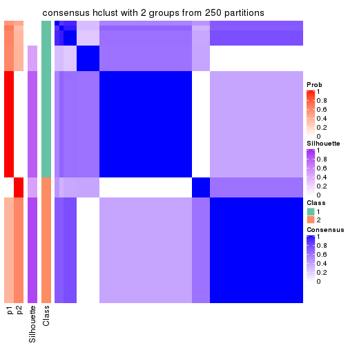
consensus_heatmap(res, k = 3)
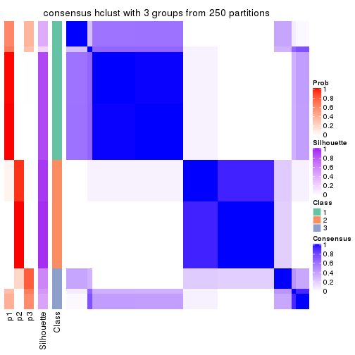
consensus_heatmap(res, k = 4)
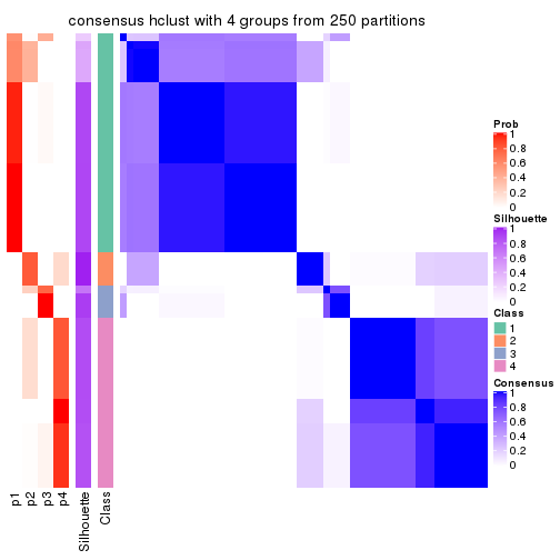
consensus_heatmap(res, k = 5)
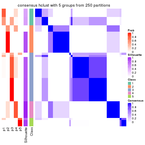
consensus_heatmap(res, k = 6)
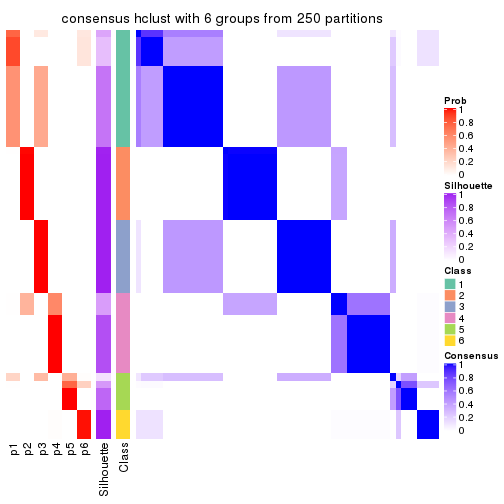
Heatmaps for the membership of samples in all partitions to see how consistent they are:
membership_heatmap(res, k = 2)
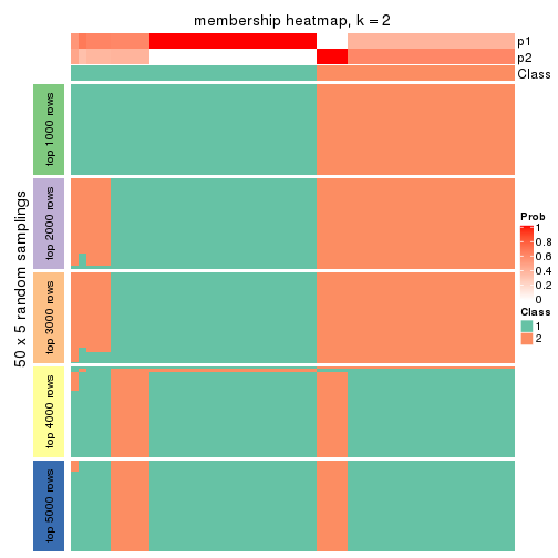
membership_heatmap(res, k = 3)
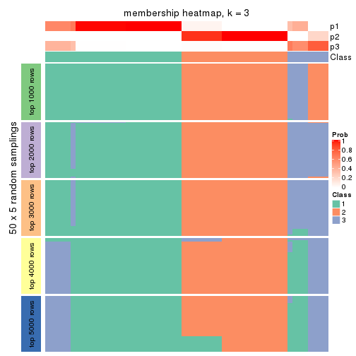
membership_heatmap(res, k = 4)
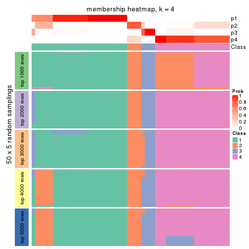
membership_heatmap(res, k = 5)
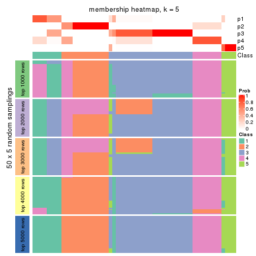
membership_heatmap(res, k = 6)
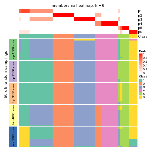
As soon as we have had the classes for columns, we can look for signatures which are significantly different between classes which can be candidate marks for certain classes. Following are the heatmaps for signatures.
Signature heatmaps where rows are scaled:
get_signatures(res, k = 2)
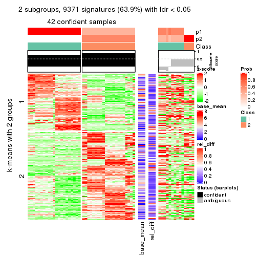
get_signatures(res, k = 3)
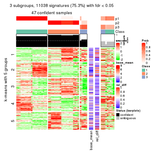
get_signatures(res, k = 4)
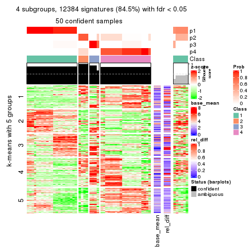
get_signatures(res, k = 5)
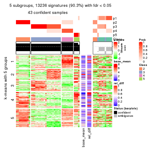
get_signatures(res, k = 6)
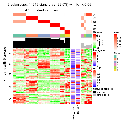
Signature heatmaps where rows are not scaled:
get_signatures(res, k = 2, scale_rows = FALSE)
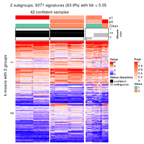
get_signatures(res, k = 3, scale_rows = FALSE)
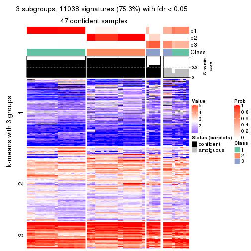
get_signatures(res, k = 4, scale_rows = FALSE)
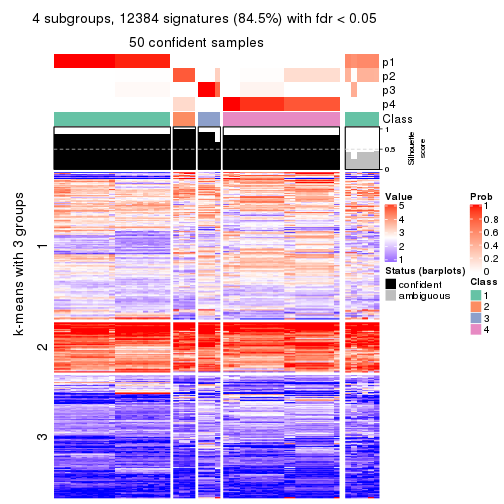
get_signatures(res, k = 5, scale_rows = FALSE)
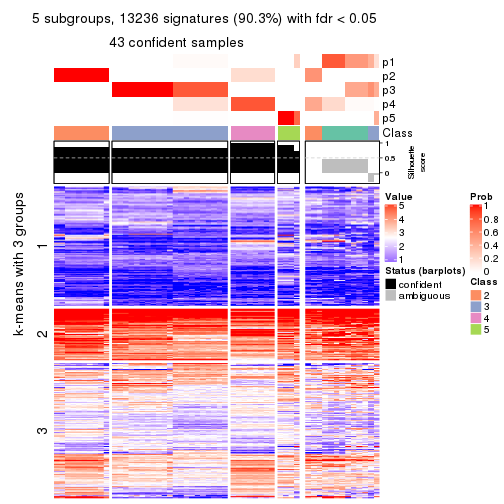
get_signatures(res, k = 6, scale_rows = FALSE)
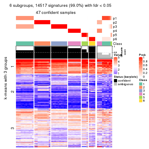
Compare the overlap of signatures from different k:
compare_signatures(res)
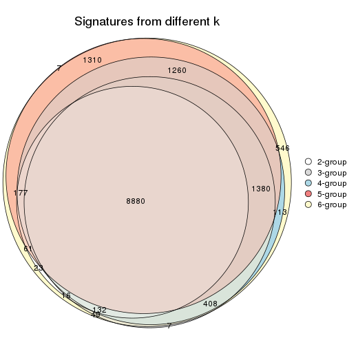
get_signature() returns a data frame invisibly. TO get the list of signatures, the function
call should be assigned to a variable explicitly. In following code, if plot argument is set
to FALSE, no heatmap is plotted while only the differential analysis is performed.
# code only for demonstration
tb = get_signature(res, k = ..., plot = FALSE)
An example of the output of tb is:
#>   which_row         fdr    mean_1    mean_2 scaled_mean_1 scaled_mean_2 km
#> 1        38 0.042760348  8.373488  9.131774    -0.5533452     0.5164555  1
#> 2        40 0.018707592  7.106213  8.469186    -0.6173731     0.5762149  1
#> 3        55 0.019134737 10.221463 11.207825    -0.6159697     0.5749050  1
#> 4        59 0.006059896  5.921854  7.869574    -0.6899429     0.6439467  1
#> 5        60 0.018055526  8.928898 10.211722    -0.6204761     0.5791110  1
#> 6        98 0.009384629 15.714769 14.887706     0.6635654    -0.6193277  2
...
The columns in tb are:
which_row: row indices corresponding to the input matrix.fdr: FDR for the differential test. mean_x: The mean value in group x.scaled_mean_x: The mean value in group x after rows are scaled.km: Row groups if k-means clustering is applied to rows.UMAP plot which shows how samples are separated.
dimension_reduction(res, k = 2, method = "UMAP")
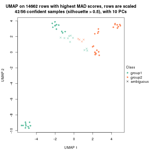
dimension_reduction(res, k = 3, method = "UMAP")
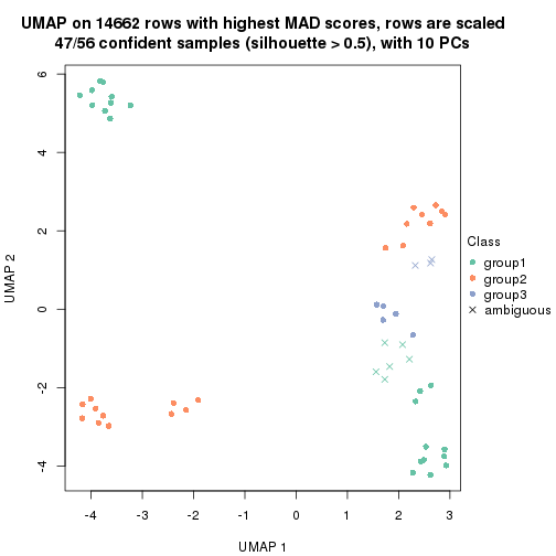
dimension_reduction(res, k = 4, method = "UMAP")
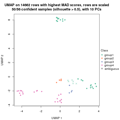
dimension_reduction(res, k = 5, method = "UMAP")
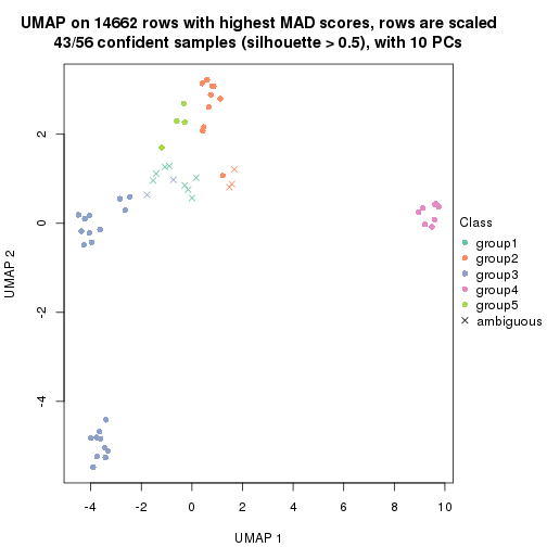
dimension_reduction(res, k = 6, method = "UMAP")
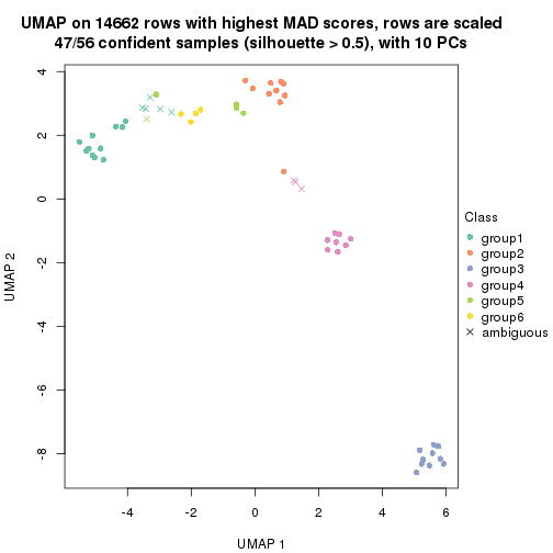
Following heatmap shows how subgroups are split when increasing k:
collect_classes(res)
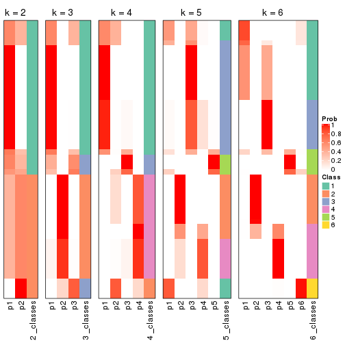
If matrix rows can be associated to genes, consider to use functional_enrichment(res,
...) to perform function enrichment for the signature genes. See this vignette for more detailed explanations.
The object with results only for a single top-value method and a single partition method can be extracted as:
res = res_list["MAD", "kmeans"]
# you can also extract it by
# res = res_list["MAD:kmeans"]
A summary of res and all the functions that can be applied to it:
res
#> A 'ConsensusPartition' object with k = 2, 3, 4, 5, 6.
#>   On a matrix with 14662 rows and 56 columns.
#>   Top rows (1000, 2000, 3000, 4000, 5000) are extracted by 'MAD' method.
#>   Subgroups are detected by 'kmeans' method.
#>   Performed in total 1250 partitions by row resampling.
#>   Best k for subgroups seems to be 2.
#>
#> Following methods can be applied to this 'ConsensusPartition' object:
#>  [1] "cola_report"             "collect_classes"         "collect_plots"
#>  [4] "collect_stats"           "colnames"                "compare_signatures"
#>  [7] "consensus_heatmap"       "dimension_reduction"     "functional_enrichment"
#> [10] "get_anno_col"            "get_anno"                "get_classes"
#> [13] "get_consensus"           "get_matrix"              "get_membership"
#> [16] "get_param"               "get_signatures"          "get_stats"
#> [19] "is_best_k"               "is_stable_k"             "membership_heatmap"
#> [22] "ncol"                    "nrow"                    "plot_ecdf"
#> [25] "rownames"                "select_partition_number" "show"
#> [28] "suggest_best_k"          "test_to_known_factors"
collect_plots() function collects all the plots made from res for all k (number of partitions)
into one single page to provide an easy and fast comparison between different k.
collect_plots(res)

The plots are:
k and the heatmap of
predicted classes for each k.k.k.k.All the plots in panels can be made by individual functions and they are plotted later in this section.
select_partition_number() produces several plots showing different
statistics for choosing “optimized” k. There are following statistics:
k;k, the area increased is defined as \(A_k - A_{k-1}\).The detailed explanations of these statistics can be found in the cola vignette.
Generally speaking, lower PAC score, higher mean silhouette score or higher
concordance corresponds to better partition. Rand index and Jaccard index
measure how similar the current partition is compared to partition with k-1.
If they are too similar, we won't accept k is better than k-1.
select_partition_number(res)
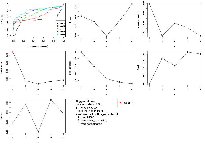
The numeric values for all these statistics can be obtained by get_stats().
get_stats(res)
#>   k 1-PAC mean_silhouette concordance area_increased  Rand Jaccard
#> 2 2 0.642           0.894       0.921         0.4895 0.491   0.491
#> 3 3 0.618           0.574       0.737         0.2923 0.842   0.687
#> 4 4 0.558           0.700       0.716         0.1238 0.738   0.401
#> 5 5 0.619           0.657       0.733         0.0774 0.929   0.726
#> 6 6 0.693           0.574       0.742         0.0531 0.902   0.586
suggest_best_k() suggests the best \(k\) based on these statistics. The rules are as follows:
suggest_best_k(res)
#> [1] 2
Following shows the table of the partitions (You need to click the show/hide
code output link to see it). The membership matrix (columns with name p*)
is inferred by
clue::cl_consensus()
function with the SE method. Basically the value in the membership matrix
represents the probability to belong to a certain group. The finall class
label for an item is determined with the group with highest probability it
belongs to.
In get_classes() function, the entropy is calculated from the membership
matrix and the silhouette score is calculated from the consensus matrix.
cbind(get_classes(res, k = 2), get_membership(res, k = 2))
#>           class entropy silhouette    p1    p2
#> SRR073723     1  0.4939      0.932 0.892 0.108
#> SRR073724     1  0.4562      0.934 0.904 0.096
#> SRR073725     1  0.4562      0.934 0.904 0.096
#> SRR073726     2  0.3274      0.915 0.060 0.940
#> SRR073727     1  0.4562      0.934 0.904 0.096
#> SRR073728     2  0.9686      0.370 0.396 0.604
#> SRR073729     2  0.9686      0.370 0.396 0.604
#> SRR073730     2  0.9686      0.370 0.396 0.604
#> SRR073731     2  0.2778      0.921 0.048 0.952
#> SRR073732     2  0.2778      0.921 0.048 0.952
#> SRR073733     2  0.2778      0.921 0.048 0.952
#> SRR073734     2  0.2778      0.921 0.048 0.952
#> SRR073735     2  0.2778      0.921 0.048 0.952
#> SRR073736     2  0.2778      0.921 0.048 0.952
#> SRR073737     2  0.2778      0.921 0.048 0.952
#> SRR073738     1  0.4562      0.934 0.904 0.096
#> SRR073739     1  0.5519      0.933 0.872 0.128
#> SRR073740     1  0.5519      0.933 0.872 0.128
#> SRR073741     1  0.5519      0.933 0.872 0.128
#> SRR073742     1  0.5519      0.933 0.872 0.128
#> SRR073743     1  0.5519      0.933 0.872 0.128
#> SRR073744     1  0.5519      0.933 0.872 0.128
#> SRR073745     1  0.5519      0.933 0.872 0.128
#> SRR073746     1  0.5519      0.933 0.872 0.128
#> SRR073747     1  0.4562      0.934 0.904 0.096
#> SRR073748     1  0.4562      0.934 0.904 0.096
#> SRR073749     1  0.4562      0.934 0.904 0.096
#> SRR073750     1  0.4562      0.934 0.904 0.096
#> SRR073751     1  0.4815      0.931 0.896 0.104
#> SRR073752     2  0.2948      0.919 0.052 0.948
#> SRR073753     2  0.2948      0.919 0.052 0.948
#> SRR073754     2  0.3274      0.915 0.060 0.940
#> SRR073755     2  0.0000      0.916 0.000 1.000
#> SRR073756     2  0.0000      0.916 0.000 1.000
#> SRR073758     2  0.0000      0.916 0.000 1.000
#> SRR073759     2  0.0938      0.917 0.012 0.988
#> SRR073760     2  0.2236      0.907 0.036 0.964
#> SRR073761     2  0.2236      0.907 0.036 0.964
#> SRR073763     2  0.2236      0.907 0.036 0.964
#> SRR073764     2  0.2236      0.907 0.036 0.964
#> SRR073765     2  0.2236      0.907 0.036 0.964
#> SRR073766     2  0.2236      0.907 0.036 0.964
#> SRR073767     2  0.2236      0.907 0.036 0.964
#> SRR073768     2  0.2236      0.907 0.036 0.964
#> SRR073769     1  0.1843      0.927 0.972 0.028
#> SRR073770     1  0.1843      0.927 0.972 0.028
#> SRR073771     1  0.1843      0.927 0.972 0.028
#> SRR073772     1  0.1843      0.927 0.972 0.028
#> SRR073773     1  0.1843      0.927 0.972 0.028
#> SRR073774     1  0.1843      0.927 0.972 0.028
#> SRR073775     1  0.1843      0.927 0.972 0.028
#> SRR073776     1  0.1843      0.927 0.972 0.028
#> SRR073777     1  0.1843      0.927 0.972 0.028
#> SRR073778     1  0.1843      0.927 0.972 0.028
#> SRR073779     2  0.3274      0.915 0.060 0.940
#> SRR073780     2  0.3274      0.915 0.060 0.940
cbind(get_classes(res, k = 3), get_membership(res, k = 3))
#>           class entropy silhouette    p1    p2    p3
#> SRR073723     1   0.650     0.0986 0.536 0.004 0.460
#> SRR073724     1   0.624     0.1433 0.560 0.000 0.440
#> SRR073725     1   0.626     0.0565 0.552 0.000 0.448
#> SRR073726     2   0.571     0.7686 0.320 0.680 0.000
#> SRR073727     1   0.624     0.1433 0.560 0.000 0.440
#> SRR073728     1   0.902    -0.0853 0.508 0.348 0.144
#> SRR073729     1   0.902    -0.0853 0.508 0.348 0.144
#> SRR073730     1   0.902    -0.0853 0.508 0.348 0.144
#> SRR073731     2   0.579     0.7907 0.332 0.668 0.000
#> SRR073732     2   0.579     0.7907 0.332 0.668 0.000
#> SRR073733     2   0.579     0.7907 0.332 0.668 0.000
#> SRR073734     2   0.579     0.7907 0.332 0.668 0.000
#> SRR073735     2   0.579     0.7907 0.332 0.668 0.000
#> SRR073736     2   0.579     0.7907 0.332 0.668 0.000
#> SRR073737     2   0.579     0.7907 0.332 0.668 0.000
#> SRR073738     1   0.623     0.1497 0.564 0.000 0.436
#> SRR073739     3   0.619     0.6127 0.292 0.016 0.692
#> SRR073740     3   0.619     0.6127 0.292 0.016 0.692
#> SRR073741     3   0.619     0.6127 0.292 0.016 0.692
#> SRR073742     3   0.619     0.6127 0.292 0.016 0.692
#> SRR073743     3   0.619     0.6127 0.292 0.016 0.692
#> SRR073744     3   0.619     0.6127 0.292 0.016 0.692
#> SRR073745     3   0.619     0.6127 0.292 0.016 0.692
#> SRR073746     3   0.667     0.4836 0.368 0.016 0.616
#> SRR073747     3   0.694     0.1919 0.468 0.016 0.516
#> SRR073748     3   0.694     0.1919 0.468 0.016 0.516
#> SRR073749     3   0.694     0.1919 0.468 0.016 0.516
#> SRR073750     1   0.624     0.1433 0.560 0.000 0.440
#> SRR073751     1   0.804     0.3415 0.636 0.116 0.248
#> SRR073752     2   0.608     0.7661 0.388 0.612 0.000
#> SRR073753     2   0.608     0.7661 0.388 0.612 0.000
#> SRR073754     2   0.629     0.6124 0.464 0.536 0.000
#> SRR073755     2   0.216     0.7818 0.064 0.936 0.000
#> SRR073756     2   0.216     0.7818 0.064 0.936 0.000
#> SRR073758     2   0.216     0.7818 0.064 0.936 0.000
#> SRR073759     2   0.588     0.7879 0.348 0.652 0.000
#> SRR073760     2   0.118     0.7709 0.012 0.976 0.012
#> SRR073761     2   0.118     0.7709 0.012 0.976 0.012
#> SRR073763     2   0.118     0.7709 0.012 0.976 0.012
#> SRR073764     2   0.118     0.7709 0.012 0.976 0.012
#> SRR073765     2   0.118     0.7709 0.012 0.976 0.012
#> SRR073766     2   0.118     0.7709 0.012 0.976 0.012
#> SRR073767     2   0.118     0.7709 0.012 0.976 0.012
#> SRR073768     2   0.118     0.7709 0.012 0.976 0.012
#> SRR073769     3   0.000     0.6831 0.000 0.000 1.000
#> SRR073770     3   0.000     0.6831 0.000 0.000 1.000
#> SRR073771     3   0.000     0.6831 0.000 0.000 1.000
#> SRR073772     3   0.000     0.6831 0.000 0.000 1.000
#> SRR073773     3   0.000     0.6831 0.000 0.000 1.000
#> SRR073774     3   0.000     0.6831 0.000 0.000 1.000
#> SRR073775     3   0.000     0.6831 0.000 0.000 1.000
#> SRR073776     3   0.000     0.6831 0.000 0.000 1.000
#> SRR073777     3   0.000     0.6831 0.000 0.000 1.000
#> SRR073778     3   0.000     0.6831 0.000 0.000 1.000
#> SRR073779     2   0.610     0.7072 0.392 0.608 0.000
#> SRR073780     2   0.610     0.7072 0.392 0.608 0.000
cbind(get_classes(res, k = 4), get_membership(res, k = 4))
#>           class entropy silhouette    p1    p2    p3    p4
#> SRR073723     1   0.488     0.5296 0.760 0.000 0.052 0.188
#> SRR073724     1   0.270     0.6271 0.876 0.000 0.000 0.124
#> SRR073725     1   0.286     0.6398 0.888 0.000 0.016 0.096
#> SRR073726     2   0.760     0.5072 0.088 0.628 0.112 0.172
#> SRR073727     1   0.270     0.6271 0.876 0.000 0.000 0.124
#> SRR073728     2   0.926     0.4388 0.176 0.444 0.140 0.240
#> SRR073729     2   0.926     0.4388 0.176 0.444 0.140 0.240
#> SRR073730     2   0.926     0.4388 0.176 0.444 0.140 0.240
#> SRR073731     2   0.000     0.6400 0.000 1.000 0.000 0.000
#> SRR073732     2   0.000     0.6400 0.000 1.000 0.000 0.000
#> SRR073733     2   0.000     0.6400 0.000 1.000 0.000 0.000
#> SRR073734     2   0.000     0.6400 0.000 1.000 0.000 0.000
#> SRR073735     2   0.000     0.6400 0.000 1.000 0.000 0.000
#> SRR073736     2   0.000     0.6400 0.000 1.000 0.000 0.000
#> SRR073737     2   0.000     0.6400 0.000 1.000 0.000 0.000
#> SRR073738     1   0.294     0.6219 0.868 0.000 0.004 0.128
#> SRR073739     1   0.540     0.5723 0.700 0.000 0.248 0.052
#> SRR073740     1   0.540     0.5723 0.700 0.000 0.248 0.052
#> SRR073741     1   0.540     0.5723 0.700 0.000 0.248 0.052
#> SRR073742     1   0.540     0.5723 0.700 0.000 0.248 0.052
#> SRR073743     1   0.540     0.5723 0.700 0.000 0.248 0.052
#> SRR073744     1   0.540     0.5723 0.700 0.000 0.248 0.052
#> SRR073745     1   0.540     0.5723 0.700 0.000 0.248 0.052
#> SRR073746     1   0.471     0.6206 0.776 0.000 0.172 0.052
#> SRR073747     1   0.234     0.6652 0.912 0.000 0.080 0.008
#> SRR073748     1   0.234     0.6652 0.912 0.000 0.080 0.008
#> SRR073749     1   0.234     0.6652 0.912 0.000 0.080 0.008
#> SRR073750     1   0.289     0.6286 0.872 0.000 0.004 0.124
#> SRR073751     1   0.924    -0.0198 0.432 0.188 0.120 0.260
#> SRR073752     2   0.358     0.6471 0.004 0.868 0.060 0.068
#> SRR073753     2   0.358     0.6471 0.004 0.868 0.060 0.068
#> SRR073754     2   0.873     0.4852 0.132 0.496 0.112 0.260
#> SRR073755     4   0.684     0.7448 0.000 0.436 0.100 0.464
#> SRR073756     4   0.684     0.7448 0.000 0.436 0.100 0.464
#> SRR073758     4   0.684     0.7448 0.000 0.436 0.100 0.464
#> SRR073759     2   0.447     0.5236 0.000 0.800 0.144 0.056
#> SRR073760     4   0.500     0.9165 0.000 0.392 0.004 0.604
#> SRR073761     4   0.500     0.9165 0.000 0.392 0.004 0.604
#> SRR073763     4   0.500     0.9165 0.000 0.392 0.004 0.604
#> SRR073764     4   0.500     0.9165 0.000 0.392 0.004 0.604
#> SRR073765     4   0.500     0.9165 0.000 0.392 0.004 0.604
#> SRR073766     4   0.500     0.9165 0.000 0.392 0.004 0.604
#> SRR073767     4   0.500     0.9165 0.000 0.392 0.004 0.604
#> SRR073768     4   0.500     0.9165 0.000 0.392 0.004 0.604
#> SRR073769     3   0.398     0.9801 0.240 0.000 0.760 0.000
#> SRR073770     3   0.511     0.9699 0.240 0.000 0.720 0.040
#> SRR073771     3   0.398     0.9801 0.240 0.000 0.760 0.000
#> SRR073772     3   0.511     0.9699 0.240 0.000 0.720 0.040
#> SRR073773     3   0.511     0.9699 0.240 0.000 0.720 0.040
#> SRR073774     3   0.398     0.9801 0.240 0.000 0.760 0.000
#> SRR073775     3   0.398     0.9801 0.240 0.000 0.760 0.000
#> SRR073776     3   0.398     0.9801 0.240 0.000 0.760 0.000
#> SRR073777     3   0.511     0.9699 0.240 0.000 0.720 0.040
#> SRR073778     3   0.398     0.9801 0.240 0.000 0.760 0.000
#> SRR073779     2   0.842     0.4985 0.112 0.536 0.112 0.240
#> SRR073780     2   0.842     0.4985 0.112 0.536 0.112 0.240
cbind(get_classes(res, k = 5), get_membership(res, k = 5))
#>           class entropy silhouette    p1    p2    p3    p4    p5
#> SRR073723     5   0.474     -0.187 0.420 0.004 0.012 0.000 0.564
#> SRR073724     1   0.450      0.390 0.564 0.000 0.008 0.000 0.428
#> SRR073725     1   0.410      0.448 0.628 0.000 0.000 0.000 0.372
#> SRR073726     2   0.715     -0.228 0.016 0.436 0.044 0.092 0.412
#> SRR073727     1   0.450      0.390 0.564 0.000 0.008 0.000 0.428
#> SRR073728     5   0.809      0.356 0.092 0.368 0.040 0.092 0.408
#> SRR073729     5   0.809      0.356 0.092 0.368 0.040 0.092 0.408
#> SRR073730     5   0.809      0.356 0.092 0.368 0.040 0.092 0.408
#> SRR073731     2   0.127      0.812 0.000 0.948 0.000 0.052 0.000
#> SRR073732     2   0.127      0.812 0.000 0.948 0.000 0.052 0.000
#> SRR073733     2   0.127      0.812 0.000 0.948 0.000 0.052 0.000
#> SRR073734     2   0.127      0.812 0.000 0.948 0.000 0.052 0.000
#> SRR073735     2   0.127      0.812 0.000 0.948 0.000 0.052 0.000
#> SRR073736     2   0.127      0.812 0.000 0.948 0.000 0.052 0.000
#> SRR073737     2   0.127      0.812 0.000 0.948 0.000 0.052 0.000
#> SRR073738     1   0.451      0.373 0.560 0.000 0.008 0.000 0.432
#> SRR073739     1   0.289      0.665 0.844 0.000 0.148 0.008 0.000
#> SRR073740     1   0.289      0.665 0.844 0.000 0.148 0.008 0.000
#> SRR073741     1   0.289      0.665 0.844 0.000 0.148 0.008 0.000
#> SRR073742     1   0.289      0.665 0.844 0.000 0.148 0.008 0.000
#> SRR073743     1   0.289      0.665 0.844 0.000 0.148 0.008 0.000
#> SRR073744     1   0.289      0.665 0.844 0.000 0.148 0.008 0.000
#> SRR073745     1   0.289      0.665 0.844 0.000 0.148 0.008 0.000
#> SRR073746     1   0.219      0.679 0.900 0.000 0.092 0.008 0.000
#> SRR073747     1   0.141      0.685 0.940 0.000 0.000 0.000 0.060
#> SRR073748     1   0.141      0.685 0.940 0.000 0.000 0.000 0.060
#> SRR073749     1   0.141      0.685 0.940 0.000 0.000 0.000 0.060
#> SRR073750     1   0.450      0.390 0.564 0.000 0.008 0.000 0.428
#> SRR073751     5   0.520      0.305 0.236 0.076 0.008 0.000 0.680
#> SRR073752     2   0.357      0.622 0.000 0.832 0.032 0.012 0.124
#> SRR073753     2   0.357      0.622 0.000 0.832 0.032 0.012 0.124
#> SRR073754     5   0.732      0.225 0.032 0.368 0.044 0.084 0.472
#> SRR073755     4   0.724      0.651 0.000 0.216 0.116 0.548 0.120
#> SRR073756     4   0.724      0.651 0.000 0.216 0.116 0.548 0.120
#> SRR073758     4   0.724      0.651 0.000 0.216 0.116 0.548 0.120
#> SRR073759     2   0.700      0.433 0.000 0.580 0.148 0.092 0.180
#> SRR073760     4   0.323      0.884 0.000 0.196 0.004 0.800 0.000
#> SRR073761     4   0.323      0.884 0.000 0.196 0.004 0.800 0.000
#> SRR073763     4   0.335      0.884 0.000 0.196 0.008 0.796 0.000
#> SRR073764     4   0.356      0.883 0.000 0.196 0.016 0.788 0.000
#> SRR073765     4   0.323      0.884 0.000 0.196 0.004 0.800 0.000
#> SRR073766     4   0.356      0.883 0.000 0.196 0.016 0.788 0.000
#> SRR073767     4   0.356      0.883 0.000 0.196 0.016 0.788 0.000
#> SRR073768     4   0.323      0.884 0.000 0.196 0.004 0.800 0.000
#> SRR073769     3   0.304      0.962 0.192 0.000 0.808 0.000 0.000
#> SRR073770     3   0.514      0.942 0.192 0.000 0.720 0.052 0.036
#> SRR073771     3   0.304      0.962 0.192 0.000 0.808 0.000 0.000
#> SRR073772     3   0.514      0.942 0.192 0.000 0.720 0.052 0.036
#> SRR073773     3   0.514      0.942 0.192 0.000 0.720 0.052 0.036
#> SRR073774     3   0.304      0.962 0.192 0.000 0.808 0.000 0.000
#> SRR073775     3   0.304      0.962 0.192 0.000 0.808 0.000 0.000
#> SRR073776     3   0.304      0.962 0.192 0.000 0.808 0.000 0.000
#> SRR073777     3   0.514      0.942 0.192 0.000 0.720 0.052 0.036
#> SRR073778     3   0.304      0.962 0.192 0.000 0.808 0.000 0.000
#> SRR073779     5   0.707      0.161 0.016 0.408 0.044 0.084 0.448
#> SRR073780     5   0.707      0.161 0.016 0.408 0.044 0.084 0.448
cbind(get_classes(res, k = 6), get_membership(res, k = 6))
#>           class entropy silhouette    p1    p2    p3    p4    p5    p6
#> SRR073723     6  0.2821     0.5294 0.116 0.004 0.020 0.000 0.004 0.856
#> SRR073724     6  0.3586     0.5037 0.216 0.000 0.028 0.000 0.000 0.756
#> SRR073725     6  0.5439     0.3103 0.296 0.016 0.032 0.000 0.044 0.612
#> SRR073726     6  0.7982    -0.1216 0.028 0.280 0.000 0.124 0.276 0.292
#> SRR073727     6  0.3586     0.5037 0.216 0.000 0.028 0.000 0.000 0.756
#> SRR073728     2  0.7840     0.1144 0.084 0.428 0.008 0.040 0.216 0.224
#> SRR073729     2  0.7840     0.1144 0.084 0.428 0.008 0.040 0.216 0.224
#> SRR073730     2  0.7840     0.1144 0.084 0.428 0.008 0.040 0.216 0.224
#> SRR073731     2  0.3126     0.4668 0.000 0.752 0.000 0.248 0.000 0.000
#> SRR073732     2  0.3126     0.4668 0.000 0.752 0.000 0.248 0.000 0.000
#> SRR073733     2  0.3126     0.4668 0.000 0.752 0.000 0.248 0.000 0.000
#> SRR073734     2  0.3126     0.4668 0.000 0.752 0.000 0.248 0.000 0.000
#> SRR073735     2  0.3126     0.4668 0.000 0.752 0.000 0.248 0.000 0.000
#> SRR073736     2  0.3126     0.4668 0.000 0.752 0.000 0.248 0.000 0.000
#> SRR073737     2  0.3126     0.4668 0.000 0.752 0.000 0.248 0.000 0.000
#> SRR073738     6  0.3409     0.5191 0.192 0.000 0.028 0.000 0.000 0.780
#> SRR073739     1  0.2260     0.8842 0.860 0.000 0.140 0.000 0.000 0.000
#> SRR073740     1  0.2260     0.8842 0.860 0.000 0.140 0.000 0.000 0.000
#> SRR073741     1  0.2260     0.8842 0.860 0.000 0.140 0.000 0.000 0.000
#> SRR073742     1  0.2260     0.8842 0.860 0.000 0.140 0.000 0.000 0.000
#> SRR073743     1  0.2260     0.8842 0.860 0.000 0.140 0.000 0.000 0.000
#> SRR073744     1  0.2260     0.8842 0.860 0.000 0.140 0.000 0.000 0.000
#> SRR073745     1  0.2260     0.8842 0.860 0.000 0.140 0.000 0.000 0.000
#> SRR073746     1  0.3639     0.8408 0.828 0.008 0.092 0.000 0.028 0.044
#> SRR073747     1  0.5570     0.6677 0.656 0.024 0.056 0.000 0.044 0.220
#> SRR073748     1  0.5570     0.6677 0.656 0.024 0.056 0.000 0.044 0.220
#> SRR073749     1  0.5570     0.6677 0.656 0.024 0.056 0.000 0.044 0.220
#> SRR073750     6  0.3586     0.5037 0.216 0.000 0.028 0.000 0.000 0.756
#> SRR073751     6  0.1994     0.5032 0.004 0.052 0.008 0.000 0.016 0.920
#> SRR073752     2  0.5860     0.1365 0.028 0.668 0.000 0.148 0.084 0.072
#> SRR073753     2  0.5860     0.1365 0.028 0.668 0.000 0.148 0.084 0.072
#> SRR073754     6  0.7722     0.0755 0.028 0.248 0.000 0.092 0.260 0.372
#> SRR073755     4  0.5065     0.1123 0.000 0.080 0.000 0.524 0.396 0.000
#> SRR073756     4  0.5065     0.1123 0.000 0.080 0.000 0.524 0.396 0.000
#> SRR073758     4  0.5065     0.1123 0.000 0.080 0.000 0.524 0.396 0.000
#> SRR073759     5  0.6797     0.0000 0.016 0.340 0.000 0.184 0.428 0.032
#> SRR073760     4  0.0146     0.8022 0.000 0.000 0.000 0.996 0.000 0.004
#> SRR073761     4  0.0146     0.8008 0.000 0.000 0.000 0.996 0.000 0.004
#> SRR073763     4  0.0405     0.8021 0.004 0.000 0.000 0.988 0.000 0.008
#> SRR073764     4  0.0914     0.7998 0.016 0.000 0.000 0.968 0.000 0.016
#> SRR073765     4  0.0000     0.8016 0.000 0.000 0.000 1.000 0.000 0.000
#> SRR073766     4  0.0914     0.7998 0.016 0.000 0.000 0.968 0.000 0.016
#> SRR073767     4  0.0914     0.7998 0.016 0.000 0.000 0.968 0.000 0.016
#> SRR073768     4  0.0291     0.8016 0.004 0.000 0.000 0.992 0.000 0.004
#> SRR073769     3  0.0000     0.9274 0.000 0.000 1.000 0.000 0.000 0.000
#> SRR073770     3  0.3219     0.8905 0.000 0.008 0.808 0.000 0.168 0.016
#> SRR073771     3  0.0458     0.9265 0.000 0.000 0.984 0.000 0.016 0.000
#> SRR073772     3  0.3502     0.8857 0.000 0.024 0.800 0.000 0.160 0.016
#> SRR073773     3  0.3183     0.8919 0.000 0.008 0.812 0.000 0.164 0.016
#> SRR073774     3  0.0260     0.9272 0.000 0.000 0.992 0.000 0.008 0.000
#> SRR073775     3  0.0000     0.9274 0.000 0.000 1.000 0.000 0.000 0.000
#> SRR073776     3  0.0000     0.9274 0.000 0.000 1.000 0.000 0.000 0.000
#> SRR073777     3  0.3502     0.8857 0.000 0.024 0.800 0.000 0.160 0.016
#> SRR073778     3  0.0000     0.9274 0.000 0.000 1.000 0.000 0.000 0.000
#> SRR073779     6  0.7782     0.0215 0.028 0.272 0.000 0.092 0.272 0.336
#> SRR073780     6  0.7782     0.0215 0.028 0.272 0.000 0.092 0.272 0.336
Heatmaps for the consensus matrix. It visualizes the probability of two samples to be in a same group.
consensus_heatmap(res, k = 2)
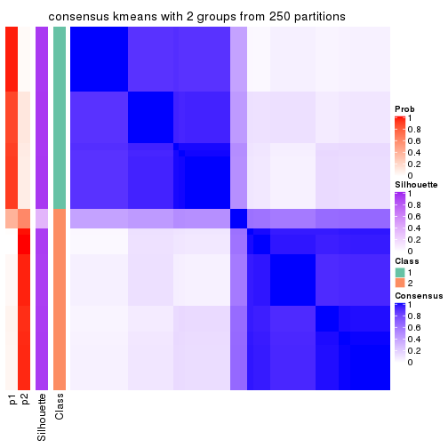
consensus_heatmap(res, k = 3)
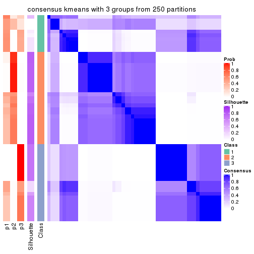
consensus_heatmap(res, k = 4)
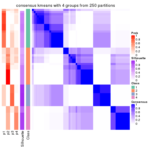
consensus_heatmap(res, k = 5)
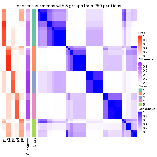
consensus_heatmap(res, k = 6)
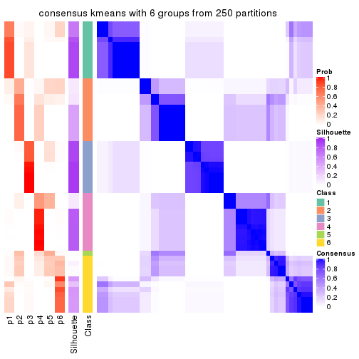
Heatmaps for the membership of samples in all partitions to see how consistent they are:
membership_heatmap(res, k = 2)

membership_heatmap(res, k = 3)
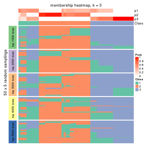
membership_heatmap(res, k = 4)
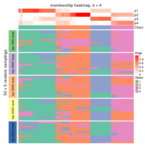
membership_heatmap(res, k = 5)
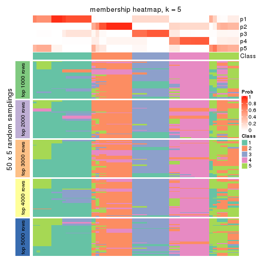
membership_heatmap(res, k = 6)
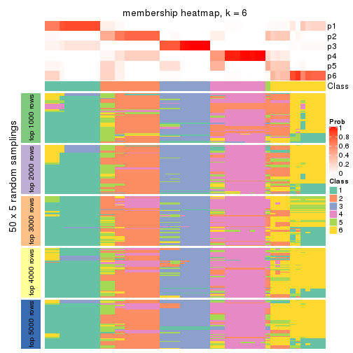
As soon as we have had the classes for columns, we can look for signatures which are significantly different between classes which can be candidate marks for certain classes. Following are the heatmaps for signatures.
Signature heatmaps where rows are scaled:
get_signatures(res, k = 2)
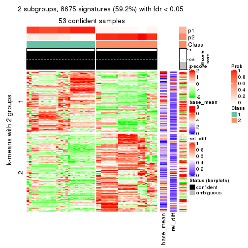
get_signatures(res, k = 3)
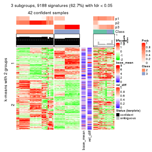
get_signatures(res, k = 4)
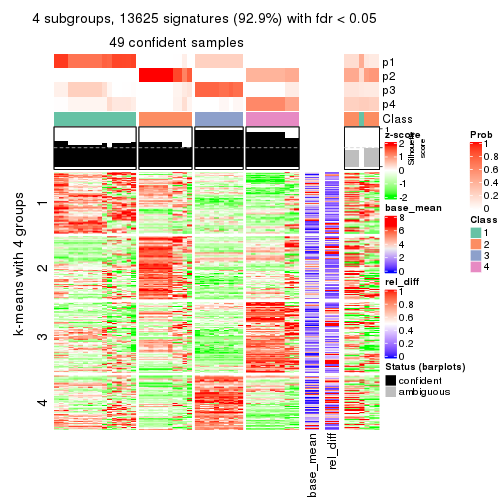
get_signatures(res, k = 5)
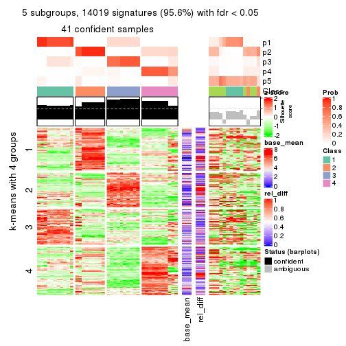
get_signatures(res, k = 6)

Signature heatmaps where rows are not scaled:
get_signatures(res, k = 2, scale_rows = FALSE)
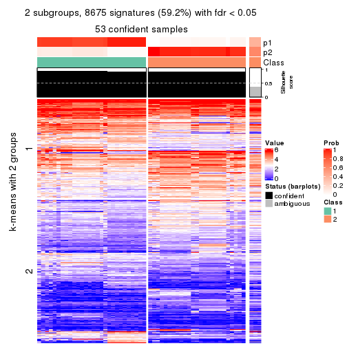
get_signatures(res, k = 3, scale_rows = FALSE)
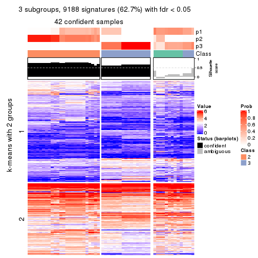
get_signatures(res, k = 4, scale_rows = FALSE)
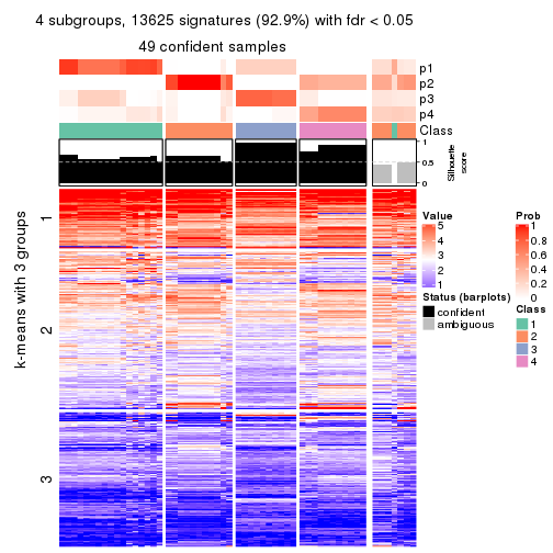
get_signatures(res, k = 5, scale_rows = FALSE)
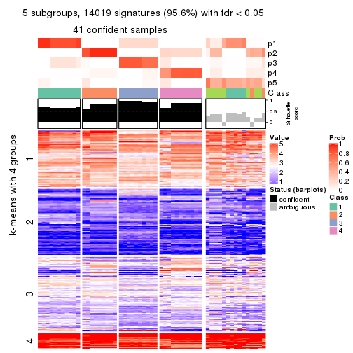
get_signatures(res, k = 6, scale_rows = FALSE)
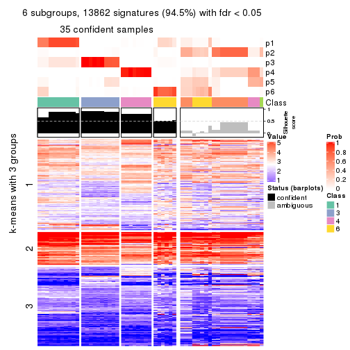
Compare the overlap of signatures from different k:
compare_signatures(res)
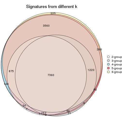
get_signature() returns a data frame invisibly. TO get the list of signatures, the function
call should be assigned to a variable explicitly. In following code, if plot argument is set
to FALSE, no heatmap is plotted while only the differential analysis is performed.
# code only for demonstration
tb = get_signature(res, k = ..., plot = FALSE)
An example of the output of tb is:
#>   which_row         fdr    mean_1    mean_2 scaled_mean_1 scaled_mean_2 km
#> 1        38 0.042760348  8.373488  9.131774    -0.5533452     0.5164555  1
#> 2        40 0.018707592  7.106213  8.469186    -0.6173731     0.5762149  1
#> 3        55 0.019134737 10.221463 11.207825    -0.6159697     0.5749050  1
#> 4        59 0.006059896  5.921854  7.869574    -0.6899429     0.6439467  1
#> 5        60 0.018055526  8.928898 10.211722    -0.6204761     0.5791110  1
#> 6        98 0.009384629 15.714769 14.887706     0.6635654    -0.6193277  2
...
The columns in tb are:
which_row: row indices corresponding to the input matrix.fdr: FDR for the differential test. mean_x: The mean value in group x.scaled_mean_x: The mean value in group x after rows are scaled.km: Row groups if k-means clustering is applied to rows.UMAP plot which shows how samples are separated.
dimension_reduction(res, k = 2, method = "UMAP")
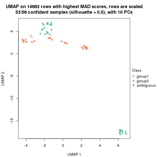
dimension_reduction(res, k = 3, method = "UMAP")
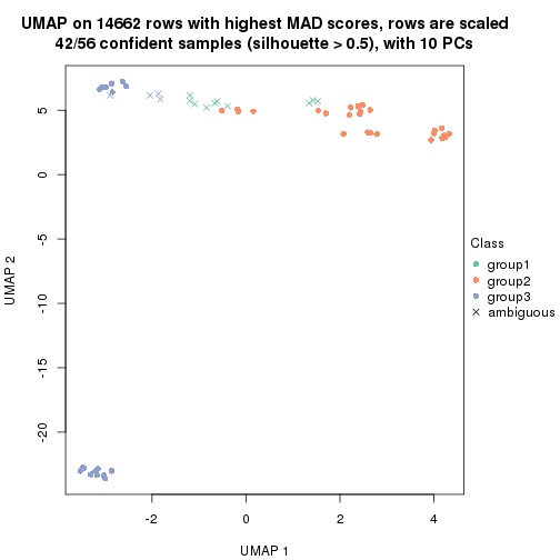
dimension_reduction(res, k = 4, method = "UMAP")
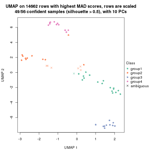
dimension_reduction(res, k = 5, method = "UMAP")

dimension_reduction(res, k = 6, method = "UMAP")
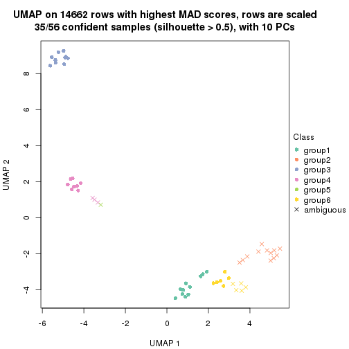
Following heatmap shows how subgroups are split when increasing k:
collect_classes(res)
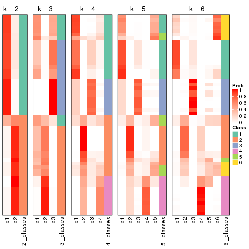
If matrix rows can be associated to genes, consider to use functional_enrichment(res,
...) to perform function enrichment for the signature genes. See this vignette for more detailed explanations.
The object with results only for a single top-value method and a single partition method can be extracted as:
res = res_list["MAD", "skmeans"]
# you can also extract it by
# res = res_list["MAD:skmeans"]
A summary of res and all the functions that can be applied to it:
res
#> A 'ConsensusPartition' object with k = 2, 3, 4, 5, 6.
#>   On a matrix with 14662 rows and 56 columns.
#>   Top rows (1000, 2000, 3000, 4000, 5000) are extracted by 'MAD' method.
#>   Subgroups are detected by 'skmeans' method.
#>   Performed in total 1250 partitions by row resampling.
#>   Best k for subgroups seems to be 3.
#>
#> Following methods can be applied to this 'ConsensusPartition' object:
#>  [1] "cola_report"             "collect_classes"         "collect_plots"
#>  [4] "collect_stats"           "colnames"                "compare_signatures"
#>  [7] "consensus_heatmap"       "dimension_reduction"     "functional_enrichment"
#> [10] "get_anno_col"            "get_anno"                "get_classes"
#> [13] "get_consensus"           "get_matrix"              "get_membership"
#> [16] "get_param"               "get_signatures"          "get_stats"
#> [19] "is_best_k"               "is_stable_k"             "membership_heatmap"
#> [22] "ncol"                    "nrow"                    "plot_ecdf"
#> [25] "rownames"                "select_partition_number" "show"
#> [28] "suggest_best_k"          "test_to_known_factors"
collect_plots() function collects all the plots made from res for all k (number of partitions)
into one single page to provide an easy and fast comparison between different k.
collect_plots(res)
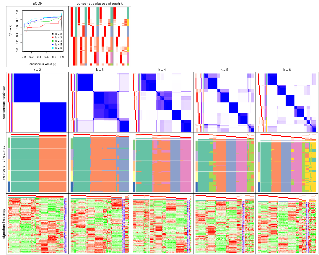
The plots are:
k and the heatmap of
predicted classes for each k.k.k.k.All the plots in panels can be made by individual functions and they are plotted later in this section.
select_partition_number() produces several plots showing different
statistics for choosing “optimized” k. There are following statistics:
k;k, the area increased is defined as \(A_k - A_{k-1}\).The detailed explanations of these statistics can be found in the cola vignette.
Generally speaking, lower PAC score, higher mean silhouette score or higher
concordance corresponds to better partition. Rand index and Jaccard index
measure how similar the current partition is compared to partition with k-1.
If they are too similar, we won't accept k is better than k-1.
select_partition_number(res)
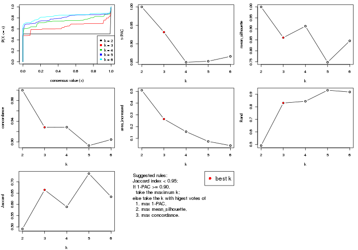
The numeric values for all these statistics can be obtained by get_stats().
get_stats(res)
#>   k 1-PAC mean_silhouette concordance area_increased  Rand Jaccard
#> 2 2 1.000           1.000       1.000         0.5096 0.491   0.491
#> 3 3 0.932           0.860       0.928         0.2646 0.831   0.665
#> 4 4 0.850           0.912       0.928         0.1570 0.844   0.589
#> 5 5 0.853           0.748       0.893         0.0742 0.932   0.737
#> 6 6 0.866           0.845       0.904         0.0386 0.918   0.634
suggest_best_k() suggests the best \(k\) based on these statistics. The rules are as follows:
suggest_best_k(res)
#> [1] 3
#> attr(,"optional")
#> [1] 2
There is also optional best \(k\) = 2 that is worth to check.
Following shows the table of the partitions (You need to click the show/hide
code output link to see it). The membership matrix (columns with name p*)
is inferred by
clue::cl_consensus()
function with the SE method. Basically the value in the membership matrix
represents the probability to belong to a certain group. The finall class
label for an item is determined with the group with highest probability it
belongs to.
In get_classes() function, the entropy is calculated from the membership
matrix and the silhouette score is calculated from the consensus matrix.
cbind(get_classes(res, k = 2), get_membership(res, k = 2))
#>           class entropy silhouette    p1    p2
#> SRR073723     1  0.0000      1.000 1.000 0.000
#> SRR073724     1  0.0000      1.000 1.000 0.000
#> SRR073725     1  0.0000      1.000 1.000 0.000
#> SRR073726     2  0.0000      1.000 0.000 1.000
#> SRR073727     1  0.0000      1.000 1.000 0.000
#> SRR073728     2  0.0000      1.000 0.000 1.000
#> SRR073729     2  0.0000      1.000 0.000 1.000
#> SRR073730     2  0.0000      1.000 0.000 1.000
#> SRR073731     2  0.0000      1.000 0.000 1.000
#> SRR073732     2  0.0000      1.000 0.000 1.000
#> SRR073733     2  0.0000      1.000 0.000 1.000
#> SRR073734     2  0.0000      1.000 0.000 1.000
#> SRR073735     2  0.0000      1.000 0.000 1.000
#> SRR073736     2  0.0000      1.000 0.000 1.000
#> SRR073737     2  0.0000      1.000 0.000 1.000
#> SRR073738     1  0.0000      1.000 1.000 0.000
#> SRR073739     1  0.0000      1.000 1.000 0.000
#> SRR073740     1  0.0000      1.000 1.000 0.000
#> SRR073741     1  0.0000      1.000 1.000 0.000
#> SRR073742     1  0.0000      1.000 1.000 0.000
#> SRR073743     1  0.0000      1.000 1.000 0.000
#> SRR073744     1  0.0000      1.000 1.000 0.000
#> SRR073745     1  0.0000      1.000 1.000 0.000
#> SRR073746     1  0.0000      1.000 1.000 0.000
#> SRR073747     1  0.0000      1.000 1.000 0.000
#> SRR073748     1  0.0000      1.000 1.000 0.000
#> SRR073749     1  0.0000      1.000 1.000 0.000
#> SRR073750     1  0.0000      1.000 1.000 0.000
#> SRR073751     1  0.0376      0.996 0.996 0.004
#> SRR073752     2  0.0000      1.000 0.000 1.000
#> SRR073753     2  0.0000      1.000 0.000 1.000
#> SRR073754     2  0.0000      1.000 0.000 1.000
#> SRR073755     2  0.0000      1.000 0.000 1.000
#> SRR073756     2  0.0000      1.000 0.000 1.000
#> SRR073758     2  0.0000      1.000 0.000 1.000
#> SRR073759     2  0.0000      1.000 0.000 1.000
#> SRR073760     2  0.0000      1.000 0.000 1.000
#> SRR073761     2  0.0000      1.000 0.000 1.000
#> SRR073763     2  0.0000      1.000 0.000 1.000
#> SRR073764     2  0.0000      1.000 0.000 1.000
#> SRR073765     2  0.0000      1.000 0.000 1.000
#> SRR073766     2  0.0000      1.000 0.000 1.000
#> SRR073767     2  0.0000      1.000 0.000 1.000
#> SRR073768     2  0.0000      1.000 0.000 1.000
#> SRR073769     1  0.0000      1.000 1.000 0.000
#> SRR073770     1  0.0000      1.000 1.000 0.000
#> SRR073771     1  0.0000      1.000 1.000 0.000
#> SRR073772     1  0.0000      1.000 1.000 0.000
#> SRR073773     1  0.0000      1.000 1.000 0.000
#> SRR073774     1  0.0000      1.000 1.000 0.000
#> SRR073775     1  0.0000      1.000 1.000 0.000
#> SRR073776     1  0.0000      1.000 1.000 0.000
#> SRR073777     1  0.0000      1.000 1.000 0.000
#> SRR073778     1  0.0000      1.000 1.000 0.000
#> SRR073779     2  0.0000      1.000 0.000 1.000
#> SRR073780     2  0.0000      1.000 0.000 1.000
cbind(get_classes(res, k = 3), get_membership(res, k = 3))
#>           class entropy silhouette    p1    p2    p3
#> SRR073723     1   0.627    0.00832 0.544 0.000 0.456
#> SRR073724     1   0.000    0.96737 1.000 0.000 0.000
#> SRR073725     1   0.000    0.96737 1.000 0.000 0.000
#> SRR073726     2   0.000    0.94208 0.000 1.000 0.000
#> SRR073727     1   0.000    0.96737 1.000 0.000 0.000
#> SRR073728     3   0.631    0.02848 0.000 0.500 0.500
#> SRR073729     2   0.631   -0.13770 0.000 0.500 0.500
#> SRR073730     3   0.631    0.02848 0.000 0.500 0.500
#> SRR073731     2   0.116    0.93768 0.000 0.972 0.028
#> SRR073732     2   0.116    0.93768 0.000 0.972 0.028
#> SRR073733     2   0.116    0.93768 0.000 0.972 0.028
#> SRR073734     2   0.116    0.93768 0.000 0.972 0.028
#> SRR073735     2   0.116    0.93768 0.000 0.972 0.028
#> SRR073736     2   0.116    0.93768 0.000 0.972 0.028
#> SRR073737     2   0.116    0.93768 0.000 0.972 0.028
#> SRR073738     1   0.000    0.96737 1.000 0.000 0.000
#> SRR073739     1   0.000    0.96737 1.000 0.000 0.000
#> SRR073740     1   0.000    0.96737 1.000 0.000 0.000
#> SRR073741     1   0.000    0.96737 1.000 0.000 0.000
#> SRR073742     1   0.000    0.96737 1.000 0.000 0.000
#> SRR073743     1   0.000    0.96737 1.000 0.000 0.000
#> SRR073744     1   0.000    0.96737 1.000 0.000 0.000
#> SRR073745     1   0.000    0.96737 1.000 0.000 0.000
#> SRR073746     1   0.000    0.96737 1.000 0.000 0.000
#> SRR073747     1   0.000    0.96737 1.000 0.000 0.000
#> SRR073748     1   0.000    0.96737 1.000 0.000 0.000
#> SRR073749     1   0.000    0.96737 1.000 0.000 0.000
#> SRR073750     1   0.000    0.96737 1.000 0.000 0.000
#> SRR073751     3   0.668    0.62054 0.216 0.060 0.724
#> SRR073752     2   0.116    0.93768 0.000 0.972 0.028
#> SRR073753     2   0.116    0.93768 0.000 0.972 0.028
#> SRR073754     2   0.000    0.94208 0.000 1.000 0.000
#> SRR073755     2   0.196    0.93825 0.000 0.944 0.056
#> SRR073756     2   0.196    0.93825 0.000 0.944 0.056
#> SRR073758     2   0.196    0.93825 0.000 0.944 0.056
#> SRR073759     2   0.196    0.94050 0.000 0.944 0.056
#> SRR073760     2   0.196    0.93825 0.000 0.944 0.056
#> SRR073761     2   0.196    0.93825 0.000 0.944 0.056
#> SRR073763     2   0.196    0.93825 0.000 0.944 0.056
#> SRR073764     2   0.196    0.93825 0.000 0.944 0.056
#> SRR073765     2   0.196    0.93825 0.000 0.944 0.056
#> SRR073766     2   0.196    0.93825 0.000 0.944 0.056
#> SRR073767     2   0.196    0.93825 0.000 0.944 0.056
#> SRR073768     2   0.196    0.93825 0.000 0.944 0.056
#> SRR073769     3   0.263    0.86635 0.084 0.000 0.916
#> SRR073770     3   0.263    0.86635 0.084 0.000 0.916
#> SRR073771     3   0.263    0.86635 0.084 0.000 0.916
#> SRR073772     3   0.263    0.86635 0.084 0.000 0.916
#> SRR073773     3   0.263    0.86635 0.084 0.000 0.916
#> SRR073774     3   0.263    0.86635 0.084 0.000 0.916
#> SRR073775     3   0.263    0.86635 0.084 0.000 0.916
#> SRR073776     3   0.263    0.86635 0.084 0.000 0.916
#> SRR073777     3   0.263    0.86635 0.084 0.000 0.916
#> SRR073778     3   0.263    0.86635 0.084 0.000 0.916
#> SRR073779     2   0.000    0.94208 0.000 1.000 0.000
#> SRR073780     2   0.000    0.94208 0.000 1.000 0.000
cbind(get_classes(res, k = 4), get_membership(res, k = 4))
#>           class entropy silhouette    p1    p2    p3    p4
#> SRR073723     1  0.5994      0.692 0.692 0.152 0.156 0.000
#> SRR073724     1  0.1940      0.932 0.924 0.076 0.000 0.000
#> SRR073725     1  0.1978      0.937 0.928 0.068 0.004 0.000
#> SRR073726     2  0.4543      0.726 0.000 0.676 0.000 0.324
#> SRR073727     1  0.1867      0.934 0.928 0.072 0.000 0.000
#> SRR073728     2  0.1229      0.791 0.008 0.968 0.004 0.020
#> SRR073729     2  0.1229      0.791 0.008 0.968 0.004 0.020
#> SRR073730     2  0.1229      0.791 0.008 0.968 0.004 0.020
#> SRR073731     2  0.3172      0.866 0.000 0.840 0.000 0.160
#> SRR073732     2  0.3172      0.866 0.000 0.840 0.000 0.160
#> SRR073733     2  0.3172      0.866 0.000 0.840 0.000 0.160
#> SRR073734     2  0.3172      0.866 0.000 0.840 0.000 0.160
#> SRR073735     2  0.3172      0.866 0.000 0.840 0.000 0.160
#> SRR073736     2  0.3172      0.866 0.000 0.840 0.000 0.160
#> SRR073737     2  0.3172      0.866 0.000 0.840 0.000 0.160
#> SRR073738     1  0.1867      0.934 0.928 0.072 0.000 0.000
#> SRR073739     1  0.0336      0.960 0.992 0.000 0.008 0.000
#> SRR073740     1  0.0336      0.960 0.992 0.000 0.008 0.000
#> SRR073741     1  0.0336      0.960 0.992 0.000 0.008 0.000
#> SRR073742     1  0.0336      0.960 0.992 0.000 0.008 0.000
#> SRR073743     1  0.0336      0.960 0.992 0.000 0.008 0.000
#> SRR073744     1  0.0336      0.960 0.992 0.000 0.008 0.000
#> SRR073745     1  0.0336      0.960 0.992 0.000 0.008 0.000
#> SRR073746     1  0.0336      0.960 0.992 0.000 0.008 0.000
#> SRR073747     1  0.0188      0.960 0.996 0.000 0.004 0.000
#> SRR073748     1  0.0188      0.960 0.996 0.000 0.004 0.000
#> SRR073749     1  0.0188      0.960 0.996 0.000 0.004 0.000
#> SRR073750     1  0.2053      0.935 0.924 0.072 0.004 0.000
#> SRR073751     2  0.2727      0.751 0.012 0.900 0.084 0.004
#> SRR073752     2  0.3123      0.866 0.000 0.844 0.000 0.156
#> SRR073753     2  0.3123      0.866 0.000 0.844 0.000 0.156
#> SRR073754     2  0.4220      0.743 0.004 0.748 0.000 0.248
#> SRR073755     4  0.0469      0.987 0.000 0.012 0.000 0.988
#> SRR073756     4  0.0469      0.987 0.000 0.012 0.000 0.988
#> SRR073758     4  0.0469      0.987 0.000 0.012 0.000 0.988
#> SRR073759     2  0.4989      0.348 0.000 0.528 0.000 0.472
#> SRR073760     4  0.0000      0.995 0.000 0.000 0.000 1.000
#> SRR073761     4  0.0000      0.995 0.000 0.000 0.000 1.000
#> SRR073763     4  0.0000      0.995 0.000 0.000 0.000 1.000
#> SRR073764     4  0.0000      0.995 0.000 0.000 0.000 1.000
#> SRR073765     4  0.0000      0.995 0.000 0.000 0.000 1.000
#> SRR073766     4  0.0000      0.995 0.000 0.000 0.000 1.000
#> SRR073767     4  0.0000      0.995 0.000 0.000 0.000 1.000
#> SRR073768     4  0.0000      0.995 0.000 0.000 0.000 1.000
#> SRR073769     3  0.0000      1.000 0.000 0.000 1.000 0.000
#> SRR073770     3  0.0000      1.000 0.000 0.000 1.000 0.000
#> SRR073771     3  0.0000      1.000 0.000 0.000 1.000 0.000
#> SRR073772     3  0.0000      1.000 0.000 0.000 1.000 0.000
#> SRR073773     3  0.0000      1.000 0.000 0.000 1.000 0.000
#> SRR073774     3  0.0000      1.000 0.000 0.000 1.000 0.000
#> SRR073775     3  0.0000      1.000 0.000 0.000 1.000 0.000
#> SRR073776     3  0.0000      1.000 0.000 0.000 1.000 0.000
#> SRR073777     3  0.0000      1.000 0.000 0.000 1.000 0.000
#> SRR073778     3  0.0000      1.000 0.000 0.000 1.000 0.000
#> SRR073779     2  0.4222      0.746 0.000 0.728 0.000 0.272
#> SRR073780     2  0.4222      0.746 0.000 0.728 0.000 0.272
cbind(get_classes(res, k = 5), get_membership(res, k = 5))
#>           class entropy silhouette    p1    p2    p3    p4    p5
#> SRR073723     5  0.2754     0.5286 0.080 0.004 0.032 0.000 0.884
#> SRR073724     1  0.4306     0.2423 0.508 0.000 0.000 0.000 0.492
#> SRR073725     1  0.4201     0.3835 0.592 0.000 0.000 0.000 0.408
#> SRR073726     2  0.6294     0.1597 0.000 0.444 0.000 0.152 0.404
#> SRR073727     1  0.4304     0.2608 0.516 0.000 0.000 0.000 0.484
#> SRR073728     5  0.3913     0.5041 0.000 0.324 0.000 0.000 0.676
#> SRR073729     5  0.3913     0.5041 0.000 0.324 0.000 0.000 0.676
#> SRR073730     5  0.3913     0.5041 0.000 0.324 0.000 0.000 0.676
#> SRR073731     2  0.0510     0.8090 0.000 0.984 0.000 0.016 0.000
#> SRR073732     2  0.0510     0.8090 0.000 0.984 0.000 0.016 0.000
#> SRR073733     2  0.0510     0.8090 0.000 0.984 0.000 0.016 0.000
#> SRR073734     2  0.0510     0.8090 0.000 0.984 0.000 0.016 0.000
#> SRR073735     2  0.0510     0.8090 0.000 0.984 0.000 0.016 0.000
#> SRR073736     2  0.0510     0.8090 0.000 0.984 0.000 0.016 0.000
#> SRR073737     2  0.0510     0.8090 0.000 0.984 0.000 0.016 0.000
#> SRR073738     5  0.4307    -0.3634 0.496 0.000 0.000 0.000 0.504
#> SRR073739     1  0.0000     0.8402 1.000 0.000 0.000 0.000 0.000
#> SRR073740     1  0.0000     0.8402 1.000 0.000 0.000 0.000 0.000
#> SRR073741     1  0.0000     0.8402 1.000 0.000 0.000 0.000 0.000
#> SRR073742     1  0.0000     0.8402 1.000 0.000 0.000 0.000 0.000
#> SRR073743     1  0.0000     0.8402 1.000 0.000 0.000 0.000 0.000
#> SRR073744     1  0.0000     0.8402 1.000 0.000 0.000 0.000 0.000
#> SRR073745     1  0.0000     0.8402 1.000 0.000 0.000 0.000 0.000
#> SRR073746     1  0.0000     0.8402 1.000 0.000 0.000 0.000 0.000
#> SRR073747     1  0.0000     0.8402 1.000 0.000 0.000 0.000 0.000
#> SRR073748     1  0.0000     0.8402 1.000 0.000 0.000 0.000 0.000
#> SRR073749     1  0.0000     0.8402 1.000 0.000 0.000 0.000 0.000
#> SRR073750     1  0.4297     0.2852 0.528 0.000 0.000 0.000 0.472
#> SRR073751     5  0.0963     0.5636 0.000 0.036 0.000 0.000 0.964
#> SRR073752     2  0.0510     0.8090 0.000 0.984 0.000 0.016 0.000
#> SRR073753     2  0.0510     0.8090 0.000 0.984 0.000 0.016 0.000
#> SRR073754     5  0.6144    -0.0275 0.000 0.332 0.000 0.148 0.520
#> SRR073755     4  0.0955     0.9738 0.000 0.004 0.000 0.968 0.028
#> SRR073756     4  0.0955     0.9738 0.000 0.004 0.000 0.968 0.028
#> SRR073758     4  0.0955     0.9738 0.000 0.004 0.000 0.968 0.028
#> SRR073759     2  0.2900     0.7037 0.000 0.864 0.000 0.108 0.028
#> SRR073760     4  0.0000     0.9903 0.000 0.000 0.000 1.000 0.000
#> SRR073761     4  0.0000     0.9903 0.000 0.000 0.000 1.000 0.000
#> SRR073763     4  0.0000     0.9903 0.000 0.000 0.000 1.000 0.000
#> SRR073764     4  0.0000     0.9903 0.000 0.000 0.000 1.000 0.000
#> SRR073765     4  0.0000     0.9903 0.000 0.000 0.000 1.000 0.000
#> SRR073766     4  0.0000     0.9903 0.000 0.000 0.000 1.000 0.000
#> SRR073767     4  0.0000     0.9903 0.000 0.000 0.000 1.000 0.000
#> SRR073768     4  0.0000     0.9903 0.000 0.000 0.000 1.000 0.000
#> SRR073769     3  0.0000     1.0000 0.000 0.000 1.000 0.000 0.000
#> SRR073770     3  0.0000     1.0000 0.000 0.000 1.000 0.000 0.000
#> SRR073771     3  0.0000     1.0000 0.000 0.000 1.000 0.000 0.000
#> SRR073772     3  0.0000     1.0000 0.000 0.000 1.000 0.000 0.000
#> SRR073773     3  0.0000     1.0000 0.000 0.000 1.000 0.000 0.000
#> SRR073774     3  0.0000     1.0000 0.000 0.000 1.000 0.000 0.000
#> SRR073775     3  0.0000     1.0000 0.000 0.000 1.000 0.000 0.000
#> SRR073776     3  0.0000     1.0000 0.000 0.000 1.000 0.000 0.000
#> SRR073777     3  0.0000     1.0000 0.000 0.000 1.000 0.000 0.000
#> SRR073778     3  0.0000     1.0000 0.000 0.000 1.000 0.000 0.000
#> SRR073779     2  0.6274     0.1282 0.000 0.432 0.000 0.148 0.420
#> SRR073780     2  0.6274     0.1282 0.000 0.432 0.000 0.148 0.420
cbind(get_classes(res, k = 6), get_membership(res, k = 6))
#>           class entropy silhouette    p1    p2    p3    p4    p5    p6
#> SRR073723     6  0.4323     -0.186 0.008 0.000 0.008 0.000 0.476 0.508
#> SRR073724     6  0.2915      0.562 0.184 0.000 0.000 0.000 0.008 0.808
#> SRR073725     6  0.3607      0.450 0.348 0.000 0.000 0.000 0.000 0.652
#> SRR073726     6  0.6835      0.366 0.000 0.200 0.000 0.096 0.212 0.492
#> SRR073727     6  0.2882      0.562 0.180 0.000 0.000 0.000 0.008 0.812
#> SRR073728     5  0.2667      1.000 0.000 0.128 0.000 0.000 0.852 0.020
#> SRR073729     5  0.2667      1.000 0.000 0.128 0.000 0.000 0.852 0.020
#> SRR073730     5  0.2667      1.000 0.000 0.128 0.000 0.000 0.852 0.020
#> SRR073731     2  0.0000      0.962 0.000 1.000 0.000 0.000 0.000 0.000
#> SRR073732     2  0.0000      0.962 0.000 1.000 0.000 0.000 0.000 0.000
#> SRR073733     2  0.0000      0.962 0.000 1.000 0.000 0.000 0.000 0.000
#> SRR073734     2  0.0000      0.962 0.000 1.000 0.000 0.000 0.000 0.000
#> SRR073735     2  0.0000      0.962 0.000 1.000 0.000 0.000 0.000 0.000
#> SRR073736     2  0.0000      0.962 0.000 1.000 0.000 0.000 0.000 0.000
#> SRR073737     2  0.0000      0.962 0.000 1.000 0.000 0.000 0.000 0.000
#> SRR073738     6  0.2981      0.559 0.160 0.000 0.000 0.000 0.020 0.820
#> SRR073739     1  0.0000      0.997 1.000 0.000 0.000 0.000 0.000 0.000
#> SRR073740     1  0.0000      0.997 1.000 0.000 0.000 0.000 0.000 0.000
#> SRR073741     1  0.0000      0.997 1.000 0.000 0.000 0.000 0.000 0.000
#> SRR073742     1  0.0000      0.997 1.000 0.000 0.000 0.000 0.000 0.000
#> SRR073743     1  0.0000      0.997 1.000 0.000 0.000 0.000 0.000 0.000
#> SRR073744     1  0.0000      0.997 1.000 0.000 0.000 0.000 0.000 0.000
#> SRR073745     1  0.0000      0.997 1.000 0.000 0.000 0.000 0.000 0.000
#> SRR073746     1  0.0000      0.997 1.000 0.000 0.000 0.000 0.000 0.000
#> SRR073747     1  0.0260      0.993 0.992 0.000 0.000 0.000 0.000 0.008
#> SRR073748     1  0.0260      0.993 0.992 0.000 0.000 0.000 0.000 0.008
#> SRR073749     1  0.0260      0.993 0.992 0.000 0.000 0.000 0.000 0.008
#> SRR073750     6  0.2915      0.562 0.184 0.000 0.000 0.000 0.008 0.808
#> SRR073751     6  0.3737      0.210 0.000 0.000 0.000 0.000 0.392 0.608
#> SRR073752     2  0.0363      0.955 0.000 0.988 0.000 0.000 0.000 0.012
#> SRR073753     2  0.0363      0.955 0.000 0.988 0.000 0.000 0.000 0.012
#> SRR073754     6  0.6319      0.410 0.000 0.140 0.000 0.096 0.188 0.576
#> SRR073755     4  0.4060      0.789 0.000 0.004 0.000 0.764 0.112 0.120
#> SRR073756     4  0.4060      0.789 0.000 0.004 0.000 0.764 0.112 0.120
#> SRR073758     4  0.4060      0.789 0.000 0.004 0.000 0.764 0.112 0.120
#> SRR073759     2  0.4514      0.658 0.000 0.744 0.000 0.024 0.124 0.108
#> SRR073760     4  0.0000      0.928 0.000 0.000 0.000 1.000 0.000 0.000
#> SRR073761     4  0.0000      0.928 0.000 0.000 0.000 1.000 0.000 0.000
#> SRR073763     4  0.0000      0.928 0.000 0.000 0.000 1.000 0.000 0.000
#> SRR073764     4  0.0000      0.928 0.000 0.000 0.000 1.000 0.000 0.000
#> SRR073765     4  0.0000      0.928 0.000 0.000 0.000 1.000 0.000 0.000
#> SRR073766     4  0.0000      0.928 0.000 0.000 0.000 1.000 0.000 0.000
#> SRR073767     4  0.0000      0.928 0.000 0.000 0.000 1.000 0.000 0.000
#> SRR073768     4  0.0000      0.928 0.000 0.000 0.000 1.000 0.000 0.000
#> SRR073769     3  0.0000      1.000 0.000 0.000 1.000 0.000 0.000 0.000
#> SRR073770     3  0.0000      1.000 0.000 0.000 1.000 0.000 0.000 0.000
#> SRR073771     3  0.0000      1.000 0.000 0.000 1.000 0.000 0.000 0.000
#> SRR073772     3  0.0000      1.000 0.000 0.000 1.000 0.000 0.000 0.000
#> SRR073773     3  0.0000      1.000 0.000 0.000 1.000 0.000 0.000 0.000
#> SRR073774     3  0.0000      1.000 0.000 0.000 1.000 0.000 0.000 0.000
#> SRR073775     3  0.0000      1.000 0.000 0.000 1.000 0.000 0.000 0.000
#> SRR073776     3  0.0000      1.000 0.000 0.000 1.000 0.000 0.000 0.000
#> SRR073777     3  0.0000      1.000 0.000 0.000 1.000 0.000 0.000 0.000
#> SRR073778     3  0.0000      1.000 0.000 0.000 1.000 0.000 0.000 0.000
#> SRR073779     6  0.6683      0.392 0.000 0.176 0.000 0.096 0.208 0.520
#> SRR073780     6  0.6683      0.392 0.000 0.176 0.000 0.096 0.208 0.520
Heatmaps for the consensus matrix. It visualizes the probability of two samples to be in a same group.
consensus_heatmap(res, k = 2)

consensus_heatmap(res, k = 3)
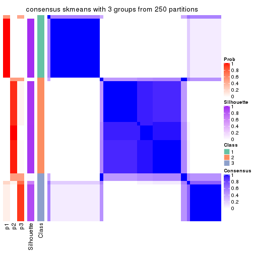
consensus_heatmap(res, k = 4)
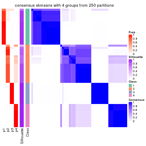
consensus_heatmap(res, k = 5)
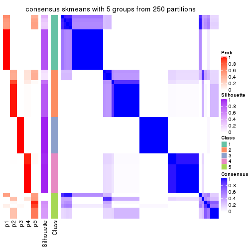
consensus_heatmap(res, k = 6)
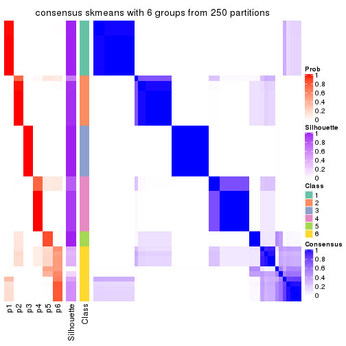
Heatmaps for the membership of samples in all partitions to see how consistent they are:
membership_heatmap(res, k = 2)

membership_heatmap(res, k = 3)
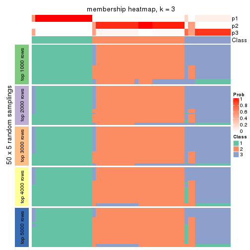
membership_heatmap(res, k = 4)
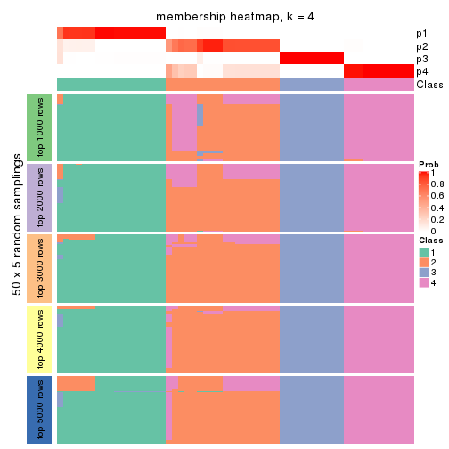
membership_heatmap(res, k = 5)
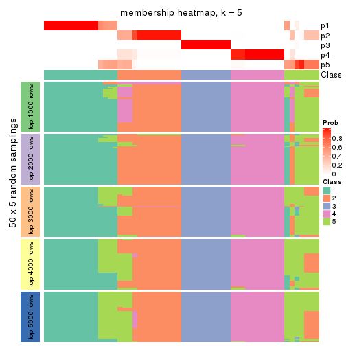
membership_heatmap(res, k = 6)
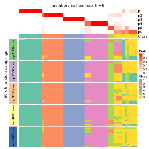
As soon as we have had the classes for columns, we can look for signatures which are significantly different between classes which can be candidate marks for certain classes. Following are the heatmaps for signatures.
Signature heatmaps where rows are scaled:
get_signatures(res, k = 2)

get_signatures(res, k = 3)
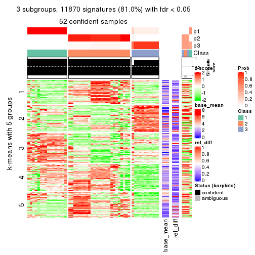
get_signatures(res, k = 4)
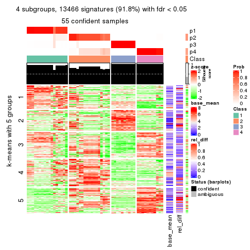
get_signatures(res, k = 5)
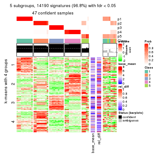
get_signatures(res, k = 6)
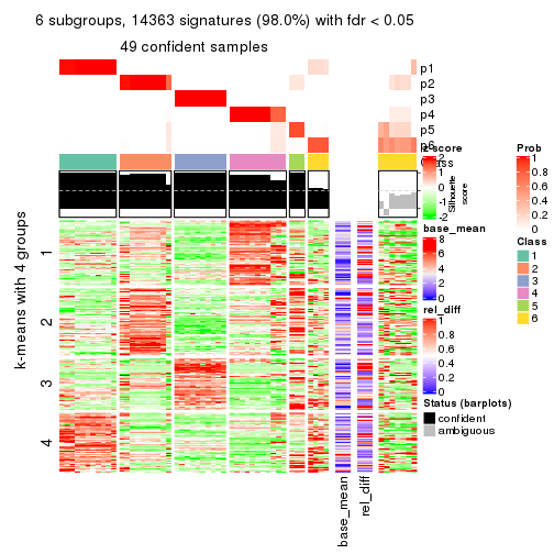
Signature heatmaps where rows are not scaled:
get_signatures(res, k = 2, scale_rows = FALSE)

get_signatures(res, k = 3, scale_rows = FALSE)
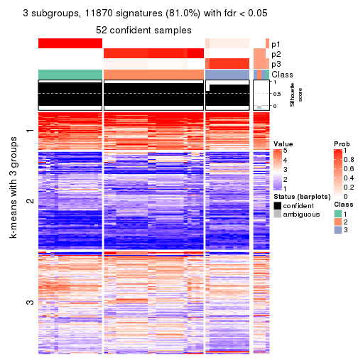
get_signatures(res, k = 4, scale_rows = FALSE)
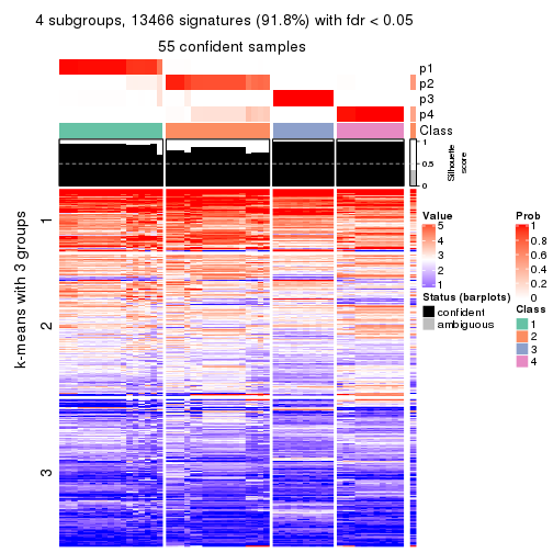
get_signatures(res, k = 5, scale_rows = FALSE)
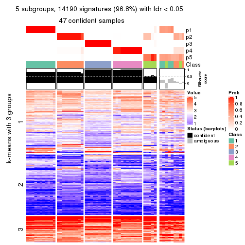
get_signatures(res, k = 6, scale_rows = FALSE)
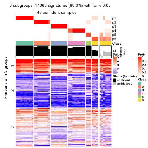
Compare the overlap of signatures from different k:
compare_signatures(res)
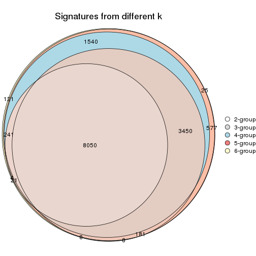
get_signature() returns a data frame invisibly. TO get the list of signatures, the function
call should be assigned to a variable explicitly. In following code, if plot argument is set
to FALSE, no heatmap is plotted while only the differential analysis is performed.
# code only for demonstration
tb = get_signature(res, k = ..., plot = FALSE)
An example of the output of tb is:
#>   which_row         fdr    mean_1    mean_2 scaled_mean_1 scaled_mean_2 km
#> 1        38 0.042760348  8.373488  9.131774    -0.5533452     0.5164555  1
#> 2        40 0.018707592  7.106213  8.469186    -0.6173731     0.5762149  1
#> 3        55 0.019134737 10.221463 11.207825    -0.6159697     0.5749050  1
#> 4        59 0.006059896  5.921854  7.869574    -0.6899429     0.6439467  1
#> 5        60 0.018055526  8.928898 10.211722    -0.6204761     0.5791110  1
#> 6        98 0.009384629 15.714769 14.887706     0.6635654    -0.6193277  2
...
The columns in tb are:
which_row: row indices corresponding to the input matrix.fdr: FDR for the differential test. mean_x: The mean value in group x.scaled_mean_x: The mean value in group x after rows are scaled.km: Row groups if k-means clustering is applied to rows.UMAP plot which shows how samples are separated.
dimension_reduction(res, k = 2, method = "UMAP")

dimension_reduction(res, k = 3, method = "UMAP")
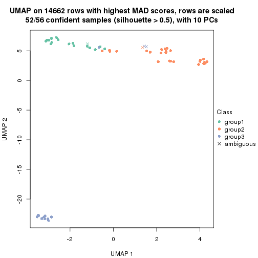
dimension_reduction(res, k = 4, method = "UMAP")
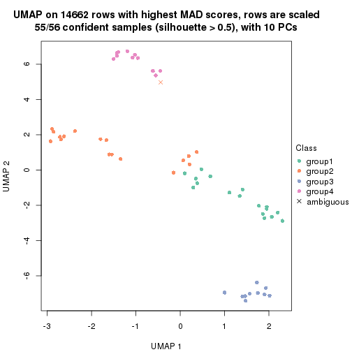
dimension_reduction(res, k = 5, method = "UMAP")
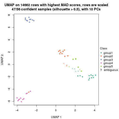
dimension_reduction(res, k = 6, method = "UMAP")
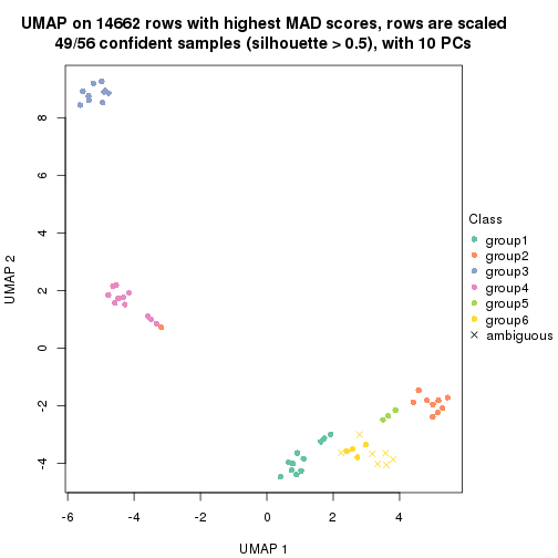
Following heatmap shows how subgroups are split when increasing k:
collect_classes(res)
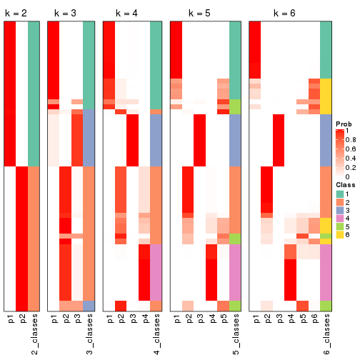
If matrix rows can be associated to genes, consider to use functional_enrichment(res,
...) to perform function enrichment for the signature genes. See this vignette for more detailed explanations.
The object with results only for a single top-value method and a single partition method can be extracted as:
res = res_list["MAD", "pam"]
# you can also extract it by
# res = res_list["MAD:pam"]
A summary of res and all the functions that can be applied to it:
res
#> A 'ConsensusPartition' object with k = 2, 3, 4, 5, 6.
#>   On a matrix with 14662 rows and 56 columns.
#>   Top rows (1000, 2000, 3000, 4000, 5000) are extracted by 'MAD' method.
#>   Subgroups are detected by 'pam' method.
#>   Performed in total 1250 partitions by row resampling.
#>   Best k for subgroups seems to be 6.
#>
#> Following methods can be applied to this 'ConsensusPartition' object:
#>  [1] "cola_report"             "collect_classes"         "collect_plots"
#>  [4] "collect_stats"           "colnames"                "compare_signatures"
#>  [7] "consensus_heatmap"       "dimension_reduction"     "functional_enrichment"
#> [10] "get_anno_col"            "get_anno"                "get_classes"
#> [13] "get_consensus"           "get_matrix"              "get_membership"
#> [16] "get_param"               "get_signatures"          "get_stats"
#> [19] "is_best_k"               "is_stable_k"             "membership_heatmap"
#> [22] "ncol"                    "nrow"                    "plot_ecdf"
#> [25] "rownames"                "select_partition_number" "show"
#> [28] "suggest_best_k"          "test_to_known_factors"
collect_plots() function collects all the plots made from res for all k (number of partitions)
into one single page to provide an easy and fast comparison between different k.
collect_plots(res)
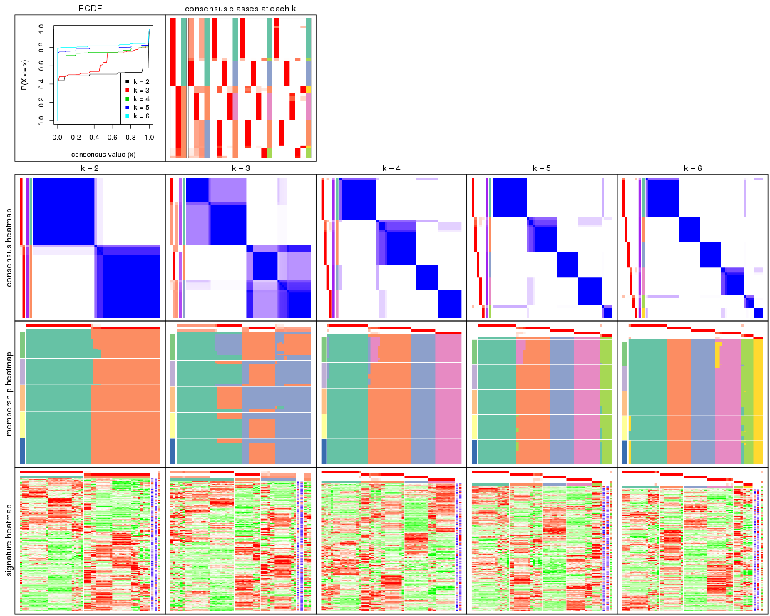
The plots are:
k and the heatmap of
predicted classes for each k.k.k.k.All the plots in panels can be made by individual functions and they are plotted later in this section.
select_partition_number() produces several plots showing different
statistics for choosing “optimized” k. There are following statistics:
k;k, the area increased is defined as \(A_k - A_{k-1}\).The detailed explanations of these statistics can be found in the cola vignette.
Generally speaking, lower PAC score, higher mean silhouette score or higher
concordance corresponds to better partition. Rand index and Jaccard index
measure how similar the current partition is compared to partition with k-1.
If they are too similar, we won't accept k is better than k-1.
select_partition_number(res)
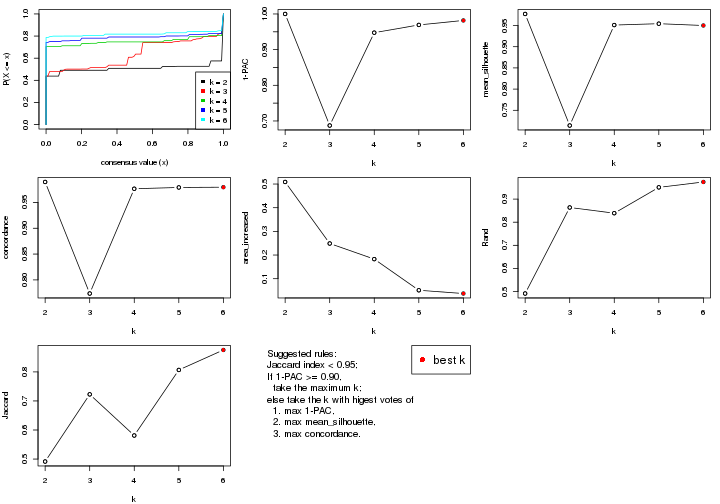
The numeric values for all these statistics can be obtained by get_stats().
get_stats(res)
#>   k 1-PAC mean_silhouette concordance area_increased  Rand Jaccard
#> 2 2 1.000           0.977       0.990         0.5087 0.492   0.492
#> 3 3 0.687           0.714       0.774         0.2487 0.864   0.723
#> 4 4 0.948           0.951       0.977         0.1827 0.839   0.581
#> 5 5 0.969           0.954       0.979         0.0510 0.951   0.807
#> 6 6 0.982           0.950       0.980         0.0373 0.974   0.875
suggest_best_k() suggests the best \(k\) based on these statistics. The rules are as follows:
suggest_best_k(res)
#> [1] 6
#> attr(,"optional")
#> [1] 2 4 5
There is also optional best \(k\) = 2 4 5 that is worth to check.
Following shows the table of the partitions (You need to click the show/hide
code output link to see it). The membership matrix (columns with name p*)
is inferred by
clue::cl_consensus()
function with the SE method. Basically the value in the membership matrix
represents the probability to belong to a certain group. The finall class
label for an item is determined with the group with highest probability it
belongs to.
In get_classes() function, the entropy is calculated from the membership
matrix and the silhouette score is calculated from the consensus matrix.
cbind(get_classes(res, k = 2), get_membership(res, k = 2))
#>           class entropy silhouette    p1    p2
#> SRR073723     1   0.000      1.000 1.000 0.000
#> SRR073724     1   0.000      1.000 1.000 0.000
#> SRR073725     1   0.000      1.000 1.000 0.000
#> SRR073726     2   0.000      0.979 0.000 1.000
#> SRR073727     1   0.000      1.000 1.000 0.000
#> SRR073728     2   0.373      0.919 0.072 0.928
#> SRR073729     2   0.402      0.911 0.080 0.920
#> SRR073730     2   0.402      0.911 0.080 0.920
#> SRR073731     2   0.000      0.979 0.000 1.000
#> SRR073732     2   0.000      0.979 0.000 1.000
#> SRR073733     2   0.000      0.979 0.000 1.000
#> SRR073734     2   0.000      0.979 0.000 1.000
#> SRR073735     2   0.000      0.979 0.000 1.000
#> SRR073736     2   0.000      0.979 0.000 1.000
#> SRR073737     2   0.000      0.979 0.000 1.000
#> SRR073738     1   0.000      1.000 1.000 0.000
#> SRR073739     1   0.000      1.000 1.000 0.000
#> SRR073740     1   0.000      1.000 1.000 0.000
#> SRR073741     1   0.000      1.000 1.000 0.000
#> SRR073742     1   0.000      1.000 1.000 0.000
#> SRR073743     1   0.000      1.000 1.000 0.000
#> SRR073744     1   0.000      1.000 1.000 0.000
#> SRR073745     1   0.000      1.000 1.000 0.000
#> SRR073746     1   0.000      1.000 1.000 0.000
#> SRR073747     1   0.000      1.000 1.000 0.000
#> SRR073748     1   0.000      1.000 1.000 0.000
#> SRR073749     1   0.000      1.000 1.000 0.000
#> SRR073750     1   0.000      1.000 1.000 0.000
#> SRR073751     2   0.929      0.497 0.344 0.656
#> SRR073752     2   0.000      0.979 0.000 1.000
#> SRR073753     2   0.000      0.979 0.000 1.000
#> SRR073754     2   0.000      0.979 0.000 1.000
#> SRR073755     2   0.000      0.979 0.000 1.000
#> SRR073756     2   0.000      0.979 0.000 1.000
#> SRR073758     2   0.000      0.979 0.000 1.000
#> SRR073759     2   0.000      0.979 0.000 1.000
#> SRR073760     2   0.000      0.979 0.000 1.000
#> SRR073761     2   0.000      0.979 0.000 1.000
#> SRR073763     2   0.000      0.979 0.000 1.000
#> SRR073764     2   0.000      0.979 0.000 1.000
#> SRR073765     2   0.000      0.979 0.000 1.000
#> SRR073766     2   0.000      0.979 0.000 1.000
#> SRR073767     2   0.000      0.979 0.000 1.000
#> SRR073768     2   0.000      0.979 0.000 1.000
#> SRR073769     1   0.000      1.000 1.000 0.000
#> SRR073770     1   0.000      1.000 1.000 0.000
#> SRR073771     1   0.000      1.000 1.000 0.000
#> SRR073772     1   0.000      1.000 1.000 0.000
#> SRR073773     1   0.000      1.000 1.000 0.000
#> SRR073774     1   0.000      1.000 1.000 0.000
#> SRR073775     1   0.000      1.000 1.000 0.000
#> SRR073776     1   0.000      1.000 1.000 0.000
#> SRR073777     1   0.000      1.000 1.000 0.000
#> SRR073778     1   0.000      1.000 1.000 0.000
#> SRR073779     2   0.000      0.979 0.000 1.000
#> SRR073780     2   0.000      0.979 0.000 1.000
cbind(get_classes(res, k = 3), get_membership(res, k = 3))
#>           class entropy silhouette    p1    p2    p3
#> SRR073723     1   0.550      0.797 0.708 0.000 0.292
#> SRR073724     1   0.629      0.839 0.536 0.000 0.464
#> SRR073725     1   0.629      0.839 0.536 0.000 0.464
#> SRR073726     2   0.631     -0.821 0.000 0.504 0.496
#> SRR073727     1   0.629      0.839 0.536 0.000 0.464
#> SRR073728     3   0.831      0.754 0.092 0.352 0.556
#> SRR073729     3   0.841      0.744 0.100 0.344 0.556
#> SRR073730     3   0.849      0.731 0.108 0.336 0.556
#> SRR073731     3   0.629      0.881 0.000 0.464 0.536
#> SRR073732     3   0.629      0.881 0.000 0.464 0.536
#> SRR073733     3   0.629      0.881 0.000 0.464 0.536
#> SRR073734     3   0.629      0.881 0.000 0.464 0.536
#> SRR073735     3   0.629      0.881 0.000 0.464 0.536
#> SRR073736     3   0.629      0.881 0.000 0.464 0.536
#> SRR073737     3   0.629      0.881 0.000 0.464 0.536
#> SRR073738     1   0.629      0.839 0.536 0.000 0.464
#> SRR073739     1   0.629      0.839 0.536 0.000 0.464
#> SRR073740     1   0.629      0.839 0.536 0.000 0.464
#> SRR073741     1   0.629      0.839 0.536 0.000 0.464
#> SRR073742     1   0.629      0.839 0.536 0.000 0.464
#> SRR073743     1   0.629      0.839 0.536 0.000 0.464
#> SRR073744     1   0.629      0.839 0.536 0.000 0.464
#> SRR073745     1   0.629      0.839 0.536 0.000 0.464
#> SRR073746     1   0.629      0.839 0.536 0.000 0.464
#> SRR073747     1   0.629      0.839 0.536 0.000 0.464
#> SRR073748     1   0.629      0.839 0.536 0.000 0.464
#> SRR073749     1   0.629      0.839 0.536 0.000 0.464
#> SRR073750     1   0.629      0.839 0.536 0.000 0.464
#> SRR073751     3   0.936      0.517 0.248 0.236 0.516
#> SRR073752     3   0.629      0.881 0.000 0.464 0.536
#> SRR073753     3   0.629      0.881 0.000 0.464 0.536
#> SRR073754     2   0.631     -0.821 0.000 0.504 0.496
#> SRR073755     2   0.000      0.785 0.000 1.000 0.000
#> SRR073756     2   0.000      0.785 0.000 1.000 0.000
#> SRR073758     2   0.000      0.785 0.000 1.000 0.000
#> SRR073759     3   0.629      0.881 0.000 0.464 0.536
#> SRR073760     2   0.000      0.785 0.000 1.000 0.000
#> SRR073761     2   0.000      0.785 0.000 1.000 0.000
#> SRR073763     2   0.000      0.785 0.000 1.000 0.000
#> SRR073764     2   0.000      0.785 0.000 1.000 0.000
#> SRR073765     2   0.000      0.785 0.000 1.000 0.000
#> SRR073766     2   0.000      0.785 0.000 1.000 0.000
#> SRR073767     2   0.000      0.785 0.000 1.000 0.000
#> SRR073768     2   0.000      0.785 0.000 1.000 0.000
#> SRR073769     1   0.000      0.722 1.000 0.000 0.000
#> SRR073770     1   0.000      0.722 1.000 0.000 0.000
#> SRR073771     1   0.000      0.722 1.000 0.000 0.000
#> SRR073772     1   0.000      0.722 1.000 0.000 0.000
#> SRR073773     1   0.000      0.722 1.000 0.000 0.000
#> SRR073774     1   0.000      0.722 1.000 0.000 0.000
#> SRR073775     1   0.000      0.722 1.000 0.000 0.000
#> SRR073776     1   0.000      0.722 1.000 0.000 0.000
#> SRR073777     1   0.000      0.722 1.000 0.000 0.000
#> SRR073778     1   0.000      0.722 1.000 0.000 0.000
#> SRR073779     3   0.631      0.824 0.000 0.492 0.508
#> SRR073780     2   0.631     -0.821 0.000 0.504 0.496
cbind(get_classes(res, k = 4), get_membership(res, k = 4))
#>           class entropy silhouette    p1    p2    p3    p4
#> SRR073723     1   0.433      0.590 0.712 0.000 0.288 0.000
#> SRR073724     1   0.000      0.982 1.000 0.000 0.000 0.000
#> SRR073725     1   0.000      0.982 1.000 0.000 0.000 0.000
#> SRR073726     2   0.361      0.785 0.000 0.800 0.000 0.200
#> SRR073727     1   0.000      0.982 1.000 0.000 0.000 0.000
#> SRR073728     2   0.000      0.939 0.000 1.000 0.000 0.000
#> SRR073729     2   0.000      0.939 0.000 1.000 0.000 0.000
#> SRR073730     2   0.000      0.939 0.000 1.000 0.000 0.000
#> SRR073731     2   0.000      0.939 0.000 1.000 0.000 0.000
#> SRR073732     2   0.000      0.939 0.000 1.000 0.000 0.000
#> SRR073733     2   0.000      0.939 0.000 1.000 0.000 0.000
#> SRR073734     2   0.000      0.939 0.000 1.000 0.000 0.000
#> SRR073735     2   0.000      0.939 0.000 1.000 0.000 0.000
#> SRR073736     2   0.000      0.939 0.000 1.000 0.000 0.000
#> SRR073737     2   0.000      0.939 0.000 1.000 0.000 0.000
#> SRR073738     1   0.000      0.982 1.000 0.000 0.000 0.000
#> SRR073739     1   0.000      0.982 1.000 0.000 0.000 0.000
#> SRR073740     1   0.000      0.982 1.000 0.000 0.000 0.000
#> SRR073741     1   0.000      0.982 1.000 0.000 0.000 0.000
#> SRR073742     1   0.000      0.982 1.000 0.000 0.000 0.000
#> SRR073743     1   0.000      0.982 1.000 0.000 0.000 0.000
#> SRR073744     1   0.000      0.982 1.000 0.000 0.000 0.000
#> SRR073745     1   0.000      0.982 1.000 0.000 0.000 0.000
#> SRR073746     1   0.000      0.982 1.000 0.000 0.000 0.000
#> SRR073747     1   0.000      0.982 1.000 0.000 0.000 0.000
#> SRR073748     1   0.000      0.982 1.000 0.000 0.000 0.000
#> SRR073749     1   0.000      0.982 1.000 0.000 0.000 0.000
#> SRR073750     1   0.000      0.982 1.000 0.000 0.000 0.000
#> SRR073751     2   0.462      0.518 0.000 0.660 0.340 0.000
#> SRR073752     2   0.000      0.939 0.000 1.000 0.000 0.000
#> SRR073753     2   0.000      0.939 0.000 1.000 0.000 0.000
#> SRR073754     2   0.361      0.785 0.000 0.800 0.000 0.200
#> SRR073755     4   0.000      1.000 0.000 0.000 0.000 1.000
#> SRR073756     4   0.000      1.000 0.000 0.000 0.000 1.000
#> SRR073758     4   0.000      1.000 0.000 0.000 0.000 1.000
#> SRR073759     2   0.000      0.939 0.000 1.000 0.000 0.000
#> SRR073760     4   0.000      1.000 0.000 0.000 0.000 1.000
#> SRR073761     4   0.000      1.000 0.000 0.000 0.000 1.000
#> SRR073763     4   0.000      1.000 0.000 0.000 0.000 1.000
#> SRR073764     4   0.000      1.000 0.000 0.000 0.000 1.000
#> SRR073765     4   0.000      1.000 0.000 0.000 0.000 1.000
#> SRR073766     4   0.000      1.000 0.000 0.000 0.000 1.000
#> SRR073767     4   0.000      1.000 0.000 0.000 0.000 1.000
#> SRR073768     4   0.000      1.000 0.000 0.000 0.000 1.000
#> SRR073769     3   0.000      1.000 0.000 0.000 1.000 0.000
#> SRR073770     3   0.000      1.000 0.000 0.000 1.000 0.000
#> SRR073771     3   0.000      1.000 0.000 0.000 1.000 0.000
#> SRR073772     3   0.000      1.000 0.000 0.000 1.000 0.000
#> SRR073773     3   0.000      1.000 0.000 0.000 1.000 0.000
#> SRR073774     3   0.000      1.000 0.000 0.000 1.000 0.000
#> SRR073775     3   0.000      1.000 0.000 0.000 1.000 0.000
#> SRR073776     3   0.000      1.000 0.000 0.000 1.000 0.000
#> SRR073777     3   0.000      1.000 0.000 0.000 1.000 0.000
#> SRR073778     3   0.000      1.000 0.000 0.000 1.000 0.000
#> SRR073779     2   0.208      0.887 0.000 0.916 0.000 0.084
#> SRR073780     2   0.361      0.785 0.000 0.800 0.000 0.200
cbind(get_classes(res, k = 5), get_membership(res, k = 5))
#>           class entropy silhouette    p1    p2    p3    p4    p5
#> SRR073723     5   0.437      0.468 0.344 0.000 0.012 0.000 0.644
#> SRR073724     1   0.000      1.000 1.000 0.000 0.000 0.000 0.000
#> SRR073725     1   0.000      1.000 1.000 0.000 0.000 0.000 0.000
#> SRR073726     2   0.311      0.780 0.000 0.800 0.000 0.200 0.000
#> SRR073727     1   0.000      1.000 1.000 0.000 0.000 0.000 0.000
#> SRR073728     5   0.000      0.895 0.000 0.000 0.000 0.000 1.000
#> SRR073729     5   0.000      0.895 0.000 0.000 0.000 0.000 1.000
#> SRR073730     5   0.000      0.895 0.000 0.000 0.000 0.000 1.000
#> SRR073731     2   0.000      0.931 0.000 1.000 0.000 0.000 0.000
#> SRR073732     2   0.000      0.931 0.000 1.000 0.000 0.000 0.000
#> SRR073733     2   0.000      0.931 0.000 1.000 0.000 0.000 0.000
#> SRR073734     2   0.000      0.931 0.000 1.000 0.000 0.000 0.000
#> SRR073735     2   0.000      0.931 0.000 1.000 0.000 0.000 0.000
#> SRR073736     2   0.000      0.931 0.000 1.000 0.000 0.000 0.000
#> SRR073737     2   0.000      0.931 0.000 1.000 0.000 0.000 0.000
#> SRR073738     1   0.000      1.000 1.000 0.000 0.000 0.000 0.000
#> SRR073739     1   0.000      1.000 1.000 0.000 0.000 0.000 0.000
#> SRR073740     1   0.000      1.000 1.000 0.000 0.000 0.000 0.000
#> SRR073741     1   0.000      1.000 1.000 0.000 0.000 0.000 0.000
#> SRR073742     1   0.000      1.000 1.000 0.000 0.000 0.000 0.000
#> SRR073743     1   0.000      1.000 1.000 0.000 0.000 0.000 0.000
#> SRR073744     1   0.000      1.000 1.000 0.000 0.000 0.000 0.000
#> SRR073745     1   0.000      1.000 1.000 0.000 0.000 0.000 0.000
#> SRR073746     1   0.000      1.000 1.000 0.000 0.000 0.000 0.000
#> SRR073747     1   0.000      1.000 1.000 0.000 0.000 0.000 0.000
#> SRR073748     1   0.000      1.000 1.000 0.000 0.000 0.000 0.000
#> SRR073749     1   0.000      1.000 1.000 0.000 0.000 0.000 0.000
#> SRR073750     1   0.000      1.000 1.000 0.000 0.000 0.000 0.000
#> SRR073751     5   0.000      0.895 0.000 0.000 0.000 0.000 1.000
#> SRR073752     2   0.000      0.931 0.000 1.000 0.000 0.000 0.000
#> SRR073753     2   0.000      0.931 0.000 1.000 0.000 0.000 0.000
#> SRR073754     2   0.534      0.648 0.000 0.668 0.000 0.200 0.132
#> SRR073755     4   0.000      1.000 0.000 0.000 0.000 1.000 0.000
#> SRR073756     4   0.000      1.000 0.000 0.000 0.000 1.000 0.000
#> SRR073758     4   0.000      1.000 0.000 0.000 0.000 1.000 0.000
#> SRR073759     2   0.000      0.931 0.000 1.000 0.000 0.000 0.000
#> SRR073760     4   0.000      1.000 0.000 0.000 0.000 1.000 0.000
#> SRR073761     4   0.000      1.000 0.000 0.000 0.000 1.000 0.000
#> SRR073763     4   0.000      1.000 0.000 0.000 0.000 1.000 0.000
#> SRR073764     4   0.000      1.000 0.000 0.000 0.000 1.000 0.000
#> SRR073765     4   0.000      1.000 0.000 0.000 0.000 1.000 0.000
#> SRR073766     4   0.000      1.000 0.000 0.000 0.000 1.000 0.000
#> SRR073767     4   0.000      1.000 0.000 0.000 0.000 1.000 0.000
#> SRR073768     4   0.000      1.000 0.000 0.000 0.000 1.000 0.000
#> SRR073769     3   0.000      1.000 0.000 0.000 1.000 0.000 0.000
#> SRR073770     3   0.000      1.000 0.000 0.000 1.000 0.000 0.000
#> SRR073771     3   0.000      1.000 0.000 0.000 1.000 0.000 0.000
#> SRR073772     3   0.000      1.000 0.000 0.000 1.000 0.000 0.000
#> SRR073773     3   0.000      1.000 0.000 0.000 1.000 0.000 0.000
#> SRR073774     3   0.000      1.000 0.000 0.000 1.000 0.000 0.000
#> SRR073775     3   0.000      1.000 0.000 0.000 1.000 0.000 0.000
#> SRR073776     3   0.000      1.000 0.000 0.000 1.000 0.000 0.000
#> SRR073777     3   0.000      1.000 0.000 0.000 1.000 0.000 0.000
#> SRR073778     3   0.000      1.000 0.000 0.000 1.000 0.000 0.000
#> SRR073779     2   0.179      0.878 0.000 0.916 0.000 0.084 0.000
#> SRR073780     2   0.311      0.780 0.000 0.800 0.000 0.200 0.000
cbind(get_classes(res, k = 6), get_membership(res, k = 6))
#>           class entropy silhouette    p1 p2    p3    p4    p5    p6
#> SRR073723     5  0.3852      0.497 0.324  0 0.012 0.000 0.664 0.000
#> SRR073724     1  0.0000      0.976 1.000  0 0.000 0.000 0.000 0.000
#> SRR073725     1  0.0000      0.976 1.000  0 0.000 0.000 0.000 0.000
#> SRR073726     6  0.0000      1.000 0.000  0 0.000 0.000 0.000 1.000
#> SRR073727     1  0.0000      0.976 1.000  0 0.000 0.000 0.000 0.000
#> SRR073728     5  0.0000      0.869 0.000  0 0.000 0.000 1.000 0.000
#> SRR073729     5  0.0000      0.869 0.000  0 0.000 0.000 1.000 0.000
#> SRR073730     5  0.0000      0.869 0.000  0 0.000 0.000 1.000 0.000
#> SRR073731     2  0.0000      1.000 0.000  1 0.000 0.000 0.000 0.000
#> SRR073732     2  0.0000      1.000 0.000  1 0.000 0.000 0.000 0.000
#> SRR073733     2  0.0000      1.000 0.000  1 0.000 0.000 0.000 0.000
#> SRR073734     2  0.0000      1.000 0.000  1 0.000 0.000 0.000 0.000
#> SRR073735     2  0.0000      1.000 0.000  1 0.000 0.000 0.000 0.000
#> SRR073736     2  0.0000      1.000 0.000  1 0.000 0.000 0.000 0.000
#> SRR073737     2  0.0000      1.000 0.000  1 0.000 0.000 0.000 0.000
#> SRR073738     1  0.3531      0.509 0.672  0 0.000 0.000 0.000 0.328
#> SRR073739     1  0.0000      0.976 1.000  0 0.000 0.000 0.000 0.000
#> SRR073740     1  0.0000      0.976 1.000  0 0.000 0.000 0.000 0.000
#> SRR073741     1  0.0000      0.976 1.000  0 0.000 0.000 0.000 0.000
#> SRR073742     1  0.0000      0.976 1.000  0 0.000 0.000 0.000 0.000
#> SRR073743     1  0.0000      0.976 1.000  0 0.000 0.000 0.000 0.000
#> SRR073744     1  0.0000      0.976 1.000  0 0.000 0.000 0.000 0.000
#> SRR073745     1  0.0000      0.976 1.000  0 0.000 0.000 0.000 0.000
#> SRR073746     1  0.0000      0.976 1.000  0 0.000 0.000 0.000 0.000
#> SRR073747     1  0.0000      0.976 1.000  0 0.000 0.000 0.000 0.000
#> SRR073748     1  0.0000      0.976 1.000  0 0.000 0.000 0.000 0.000
#> SRR073749     1  0.0000      0.976 1.000  0 0.000 0.000 0.000 0.000
#> SRR073750     1  0.0000      0.976 1.000  0 0.000 0.000 0.000 0.000
#> SRR073751     5  0.0632      0.855 0.000  0 0.000 0.000 0.976 0.024
#> SRR073752     2  0.0000      1.000 0.000  1 0.000 0.000 0.000 0.000
#> SRR073753     2  0.0000      1.000 0.000  1 0.000 0.000 0.000 0.000
#> SRR073754     6  0.0000      1.000 0.000  0 0.000 0.000 0.000 1.000
#> SRR073755     4  0.0790      0.934 0.000  0 0.000 0.968 0.000 0.032
#> SRR073756     4  0.2883      0.767 0.000  0 0.000 0.788 0.000 0.212
#> SRR073758     4  0.2883      0.767 0.000  0 0.000 0.788 0.000 0.212
#> SRR073759     2  0.0000      1.000 0.000  1 0.000 0.000 0.000 0.000
#> SRR073760     4  0.0000      0.953 0.000  0 0.000 1.000 0.000 0.000
#> SRR073761     4  0.0000      0.953 0.000  0 0.000 1.000 0.000 0.000
#> SRR073763     4  0.0000      0.953 0.000  0 0.000 1.000 0.000 0.000
#> SRR073764     4  0.0000      0.953 0.000  0 0.000 1.000 0.000 0.000
#> SRR073765     4  0.0000      0.953 0.000  0 0.000 1.000 0.000 0.000
#> SRR073766     4  0.0000      0.953 0.000  0 0.000 1.000 0.000 0.000
#> SRR073767     4  0.0000      0.953 0.000  0 0.000 1.000 0.000 0.000
#> SRR073768     4  0.0000      0.953 0.000  0 0.000 1.000 0.000 0.000
#> SRR073769     3  0.0000      1.000 0.000  0 1.000 0.000 0.000 0.000
#> SRR073770     3  0.0000      1.000 0.000  0 1.000 0.000 0.000 0.000
#> SRR073771     3  0.0000      1.000 0.000  0 1.000 0.000 0.000 0.000
#> SRR073772     3  0.0000      1.000 0.000  0 1.000 0.000 0.000 0.000
#> SRR073773     3  0.0000      1.000 0.000  0 1.000 0.000 0.000 0.000
#> SRR073774     3  0.0000      1.000 0.000  0 1.000 0.000 0.000 0.000
#> SRR073775     3  0.0000      1.000 0.000  0 1.000 0.000 0.000 0.000
#> SRR073776     3  0.0000      1.000 0.000  0 1.000 0.000 0.000 0.000
#> SRR073777     3  0.0000      1.000 0.000  0 1.000 0.000 0.000 0.000
#> SRR073778     3  0.0000      1.000 0.000  0 1.000 0.000 0.000 0.000
#> SRR073779     6  0.0000      1.000 0.000  0 0.000 0.000 0.000 1.000
#> SRR073780     6  0.0000      1.000 0.000  0 0.000 0.000 0.000 1.000
Heatmaps for the consensus matrix. It visualizes the probability of two samples to be in a same group.
consensus_heatmap(res, k = 2)
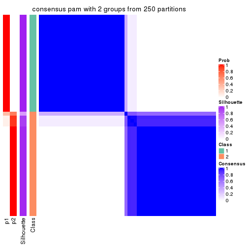
consensus_heatmap(res, k = 3)
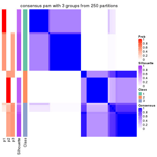
consensus_heatmap(res, k = 4)
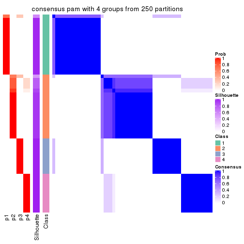
consensus_heatmap(res, k = 5)
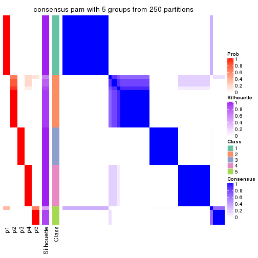
consensus_heatmap(res, k = 6)
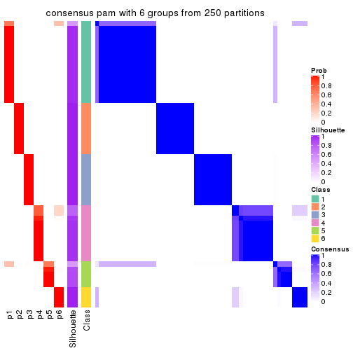
Heatmaps for the membership of samples in all partitions to see how consistent they are:
membership_heatmap(res, k = 2)
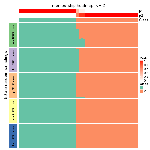
membership_heatmap(res, k = 3)
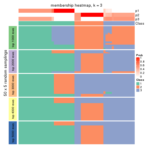
membership_heatmap(res, k = 4)
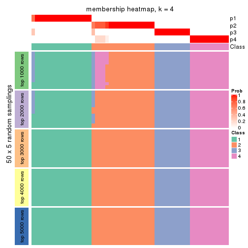
membership_heatmap(res, k = 5)
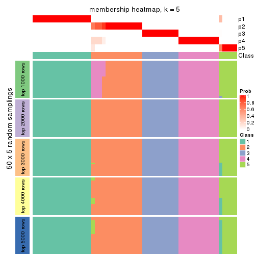
membership_heatmap(res, k = 6)
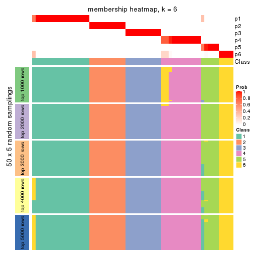
As soon as we have had the classes for columns, we can look for signatures which are significantly different between classes which can be candidate marks for certain classes. Following are the heatmaps for signatures.
Signature heatmaps where rows are scaled:
get_signatures(res, k = 2)
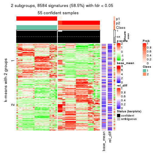
get_signatures(res, k = 3)
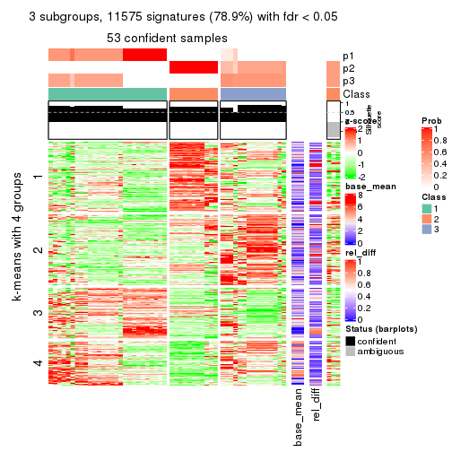
get_signatures(res, k = 4)
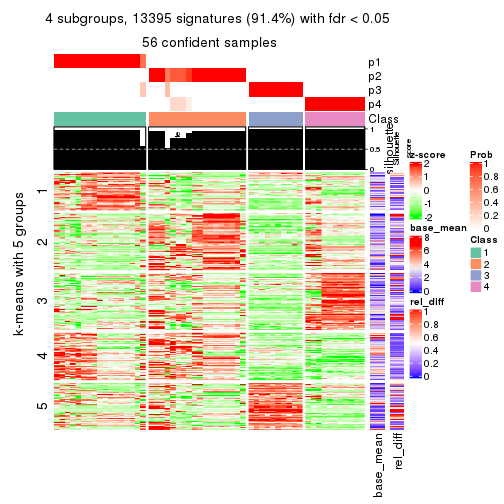
get_signatures(res, k = 5)
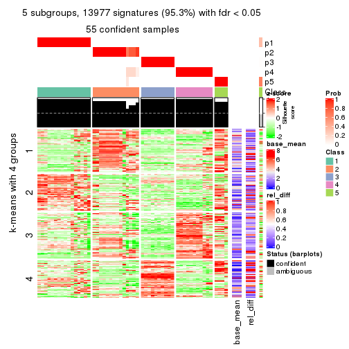
get_signatures(res, k = 6)
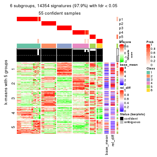
Signature heatmaps where rows are not scaled:
get_signatures(res, k = 2, scale_rows = FALSE)
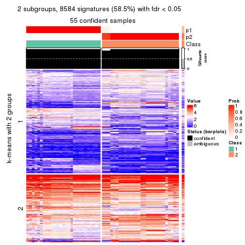
get_signatures(res, k = 3, scale_rows = FALSE)
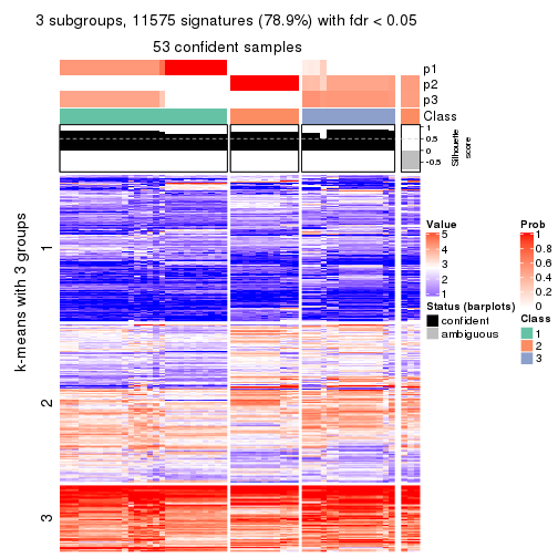
get_signatures(res, k = 4, scale_rows = FALSE)
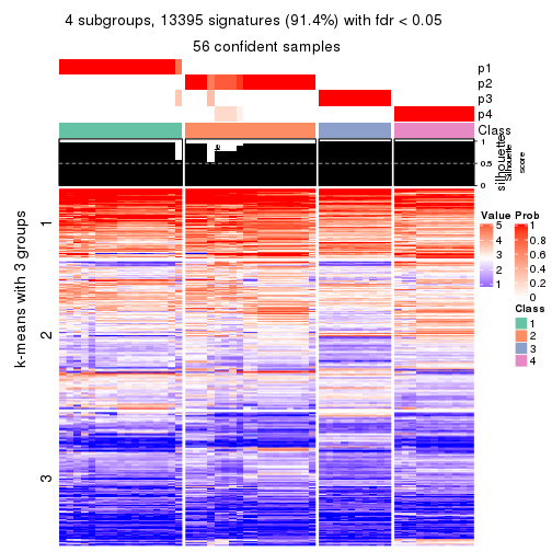
get_signatures(res, k = 5, scale_rows = FALSE)
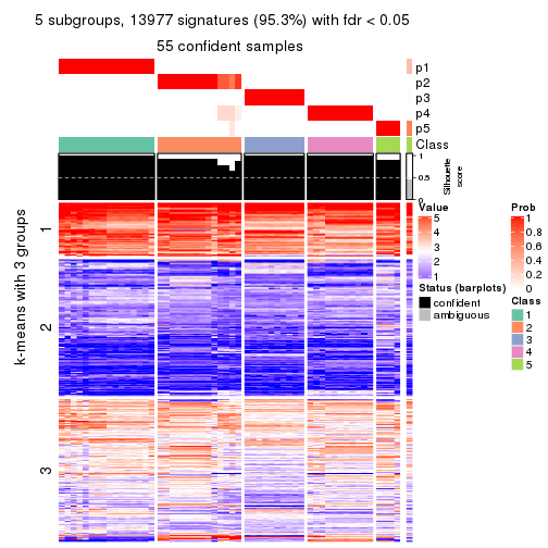
get_signatures(res, k = 6, scale_rows = FALSE)
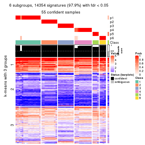
Compare the overlap of signatures from different k:
compare_signatures(res)
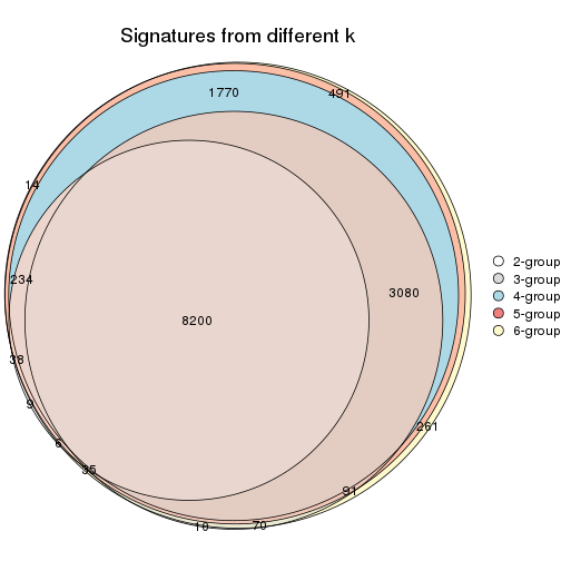
get_signature() returns a data frame invisibly. TO get the list of signatures, the function
call should be assigned to a variable explicitly. In following code, if plot argument is set
to FALSE, no heatmap is plotted while only the differential analysis is performed.
# code only for demonstration
tb = get_signature(res, k = ..., plot = FALSE)
An example of the output of tb is:
#>   which_row         fdr    mean_1    mean_2 scaled_mean_1 scaled_mean_2 km
#> 1        38 0.042760348  8.373488  9.131774    -0.5533452     0.5164555  1
#> 2        40 0.018707592  7.106213  8.469186    -0.6173731     0.5762149  1
#> 3        55 0.019134737 10.221463 11.207825    -0.6159697     0.5749050  1
#> 4        59 0.006059896  5.921854  7.869574    -0.6899429     0.6439467  1
#> 5        60 0.018055526  8.928898 10.211722    -0.6204761     0.5791110  1
#> 6        98 0.009384629 15.714769 14.887706     0.6635654    -0.6193277  2
...
The columns in tb are:
which_row: row indices corresponding to the input matrix.fdr: FDR for the differential test. mean_x: The mean value in group x.scaled_mean_x: The mean value in group x after rows are scaled.km: Row groups if k-means clustering is applied to rows.UMAP plot which shows how samples are separated.
dimension_reduction(res, k = 2, method = "UMAP")
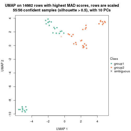
dimension_reduction(res, k = 3, method = "UMAP")
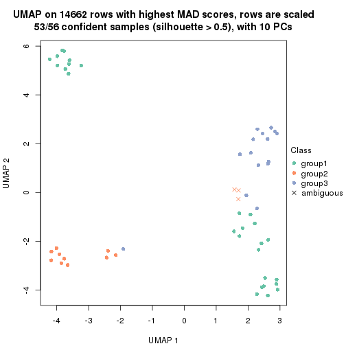
dimension_reduction(res, k = 4, method = "UMAP")
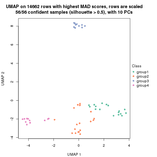
dimension_reduction(res, k = 5, method = "UMAP")
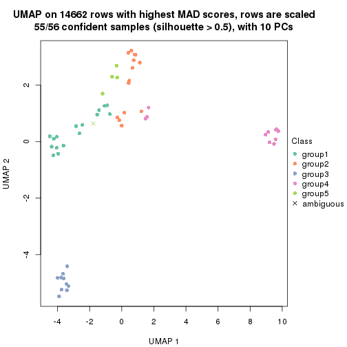
dimension_reduction(res, k = 6, method = "UMAP")
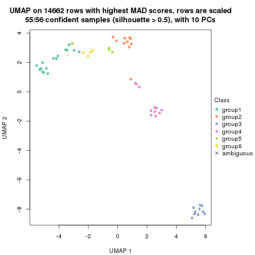
Following heatmap shows how subgroups are split when increasing k:
collect_classes(res)
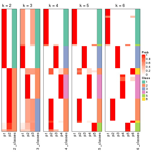
If matrix rows can be associated to genes, consider to use functional_enrichment(res,
...) to perform function enrichment for the signature genes. See this vignette for more detailed explanations.
The object with results only for a single top-value method and a single partition method can be extracted as:
res = res_list["MAD", "mclust"]
# you can also extract it by
# res = res_list["MAD:mclust"]
A summary of res and all the functions that can be applied to it:
res
#> A 'ConsensusPartition' object with k = 2, 3, 4, 5, 6.
#>   On a matrix with 14662 rows and 56 columns.
#>   Top rows (1000, 2000, 3000, 4000, 5000) are extracted by 'MAD' method.
#>   Subgroups are detected by 'mclust' method.
#>   Performed in total 1250 partitions by row resampling.
#>   Best k for subgroups seems to be 6.
#>
#> Following methods can be applied to this 'ConsensusPartition' object:
#>  [1] "cola_report"             "collect_classes"         "collect_plots"
#>  [4] "collect_stats"           "colnames"                "compare_signatures"
#>  [7] "consensus_heatmap"       "dimension_reduction"     "functional_enrichment"
#> [10] "get_anno_col"            "get_anno"                "get_classes"
#> [13] "get_consensus"           "get_matrix"              "get_membership"
#> [16] "get_param"               "get_signatures"          "get_stats"
#> [19] "is_best_k"               "is_stable_k"             "membership_heatmap"
#> [22] "ncol"                    "nrow"                    "plot_ecdf"
#> [25] "rownames"                "select_partition_number" "show"
#> [28] "suggest_best_k"          "test_to_known_factors"
collect_plots() function collects all the plots made from res for all k (number of partitions)
into one single page to provide an easy and fast comparison between different k.
collect_plots(res)
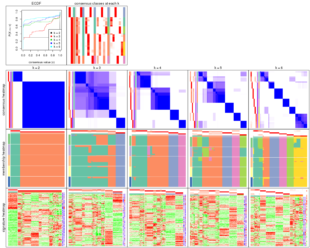
The plots are:
k and the heatmap of
predicted classes for each k.k.k.k.All the plots in panels can be made by individual functions and they are plotted later in this section.
select_partition_number() produces several plots showing different
statistics for choosing “optimized” k. There are following statistics:
k;k, the area increased is defined as \(A_k - A_{k-1}\).The detailed explanations of these statistics can be found in the cola vignette.
Generally speaking, lower PAC score, higher mean silhouette score or higher
concordance corresponds to better partition. Rand index and Jaccard index
measure how similar the current partition is compared to partition with k-1.
If they are too similar, we won't accept k is better than k-1.
select_partition_number(res)
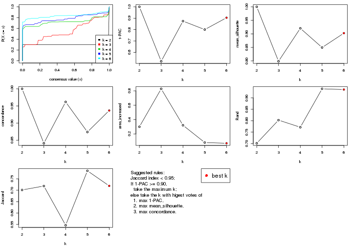
The numeric values for all these statistics can be obtained by get_stats().
get_stats(res)
#>   k 1-PAC mean_silhouette concordance area_increased  Rand Jaccard
#> 2 2 1.000           1.000       1.000         0.2994 0.701   0.701
#> 3 3 0.522           0.799       0.841         0.8281 0.803   0.719
#> 4 4 0.874           0.921       0.962         0.3204 0.771   0.546
#> 5 5 0.800           0.850       0.874         0.0799 0.940   0.785
#> 6 6 0.904           0.903       0.937         0.0697 0.936   0.719
suggest_best_k() suggests the best \(k\) based on these statistics. The rules are as follows:
suggest_best_k(res)
#> [1] 6
#> attr(,"optional")
#> [1] 2
There is also optional best \(k\) = 2 that is worth to check.
Following shows the table of the partitions (You need to click the show/hide
code output link to see it). The membership matrix (columns with name p*)
is inferred by
clue::cl_consensus()
function with the SE method. Basically the value in the membership matrix
represents the probability to belong to a certain group. The finall class
label for an item is determined with the group with highest probability it
belongs to.
In get_classes() function, the entropy is calculated from the membership
matrix and the silhouette score is calculated from the consensus matrix.
cbind(get_classes(res, k = 2), get_membership(res, k = 2))
#>           class entropy silhouette p1 p2
#> SRR073723     2       0          1  0  1
#> SRR073724     2       0          1  0  1
#> SRR073725     2       0          1  0  1
#> SRR073726     2       0          1  0  1
#> SRR073727     2       0          1  0  1
#> SRR073728     2       0          1  0  1
#> SRR073729     2       0          1  0  1
#> SRR073730     2       0          1  0  1
#> SRR073731     2       0          1  0  1
#> SRR073732     2       0          1  0  1
#> SRR073733     2       0          1  0  1
#> SRR073734     2       0          1  0  1
#> SRR073735     2       0          1  0  1
#> SRR073736     2       0          1  0  1
#> SRR073737     2       0          1  0  1
#> SRR073738     2       0          1  0  1
#> SRR073739     2       0          1  0  1
#> SRR073740     2       0          1  0  1
#> SRR073741     2       0          1  0  1
#> SRR073742     2       0          1  0  1
#> SRR073743     2       0          1  0  1
#> SRR073744     2       0          1  0  1
#> SRR073745     2       0          1  0  1
#> SRR073746     2       0          1  0  1
#> SRR073747     2       0          1  0  1
#> SRR073748     2       0          1  0  1
#> SRR073749     2       0          1  0  1
#> SRR073750     2       0          1  0  1
#> SRR073751     2       0          1  0  1
#> SRR073752     2       0          1  0  1
#> SRR073753     2       0          1  0  1
#> SRR073754     2       0          1  0  1
#> SRR073755     2       0          1  0  1
#> SRR073756     2       0          1  0  1
#> SRR073758     2       0          1  0  1
#> SRR073759     2       0          1  0  1
#> SRR073760     2       0          1  0  1
#> SRR073761     2       0          1  0  1
#> SRR073763     2       0          1  0  1
#> SRR073764     2       0          1  0  1
#> SRR073765     2       0          1  0  1
#> SRR073766     2       0          1  0  1
#> SRR073767     2       0          1  0  1
#> SRR073768     2       0          1  0  1
#> SRR073769     1       0          1  1  0
#> SRR073770     1       0          1  1  0
#> SRR073771     1       0          1  1  0
#> SRR073772     1       0          1  1  0
#> SRR073773     1       0          1  1  0
#> SRR073774     1       0          1  1  0
#> SRR073775     1       0          1  1  0
#> SRR073776     1       0          1  1  0
#> SRR073777     1       0          1  1  0
#> SRR073778     1       0          1  1  0
#> SRR073779     2       0          1  0  1
#> SRR073780     2       0          1  0  1
cbind(get_classes(res, k = 3), get_membership(res, k = 3))
#> class entropy silhouette p1 p2 p3
#> SRR073723 1 0.420 0.748 0.864 0.112 0.024
#> SRR073724 1 0.441 0.731 0.824 0.172 0.004
#> SRR073725 1 0.590 0.682 0.648 0.352 0.000
#> SRR073726 1 0.175 0.746 0.952 0.048 0.000
#> SRR073727 1 0.512 0.730 0.812 0.160 0.028
#> SRR073728 1 0.127 0.748 0.972 0.004 0.024
#> SRR073729 1 0.127 0.748 0.972 0.004 0.024
#> SRR073730 1 0.127 0.748 0.972 0.004 0.024
#> SRR073731 1 0.175 0.746 0.952 0.048 0.000
#> SRR073732 1 0.175 0.746 0.952 0.048 0.000
#> SRR073733 1 0.175 0.746 0.952 0.048 0.000
#> SRR073734 1 0.175 0.746 0.952 0.048 0.000
#> SRR073735 1 0.175 0.746 0.952 0.048 0.000
#> SRR073736 1 0.175 0.746 0.952 0.048 0.000
#> SRR073737 1 0.175 0.746 0.952 0.048 0.000
#> SRR073738 1 0.441 0.731 0.824 0.172 0.004
#> SRR073739 1 0.599 0.677 0.632 0.368 0.000
#> SRR073740 1 0.599 0.677 0.632 0.368 0.000
#> SRR073741 1 0.599 0.677 0.632 0.368 0.000
#> SRR073742 1 0.599 0.677 0.632 0.368 0.000
#> SRR073743 1 0.599 0.677 0.632 0.368 0.000
#> SRR073744 1 0.599 0.677 0.632 0.368 0.000
#> SRR073745 1 0.599 0.677 0.632 0.368 0.000
#> SRR073746 1 0.599 0.677 0.632 0.368 0.000
#> SRR073747 1 0.599 0.677 0.632 0.368 0.000
#> SRR073748 1 0.599 0.677 0.632 0.368 0.000
#> SRR073749 1 0.599 0.677 0.632 0.368 0.000
#> SRR073750 1 0.424 0.731 0.824 0.176 0.000
#> SRR073751 1 0.127 0.748 0.972 0.004 0.024
#> SRR073752 1 0.141 0.749 0.964 0.036 0.000
#> SRR073753 1 0.141 0.749 0.964 0.036 0.000
#> SRR073754 1 0.175 0.746 0.952 0.048 0.000
#> SRR073755 1 0.590 0.510 0.648 0.352 0.000
#> SRR073756 1 0.590 0.510 0.648 0.352 0.000
#> SRR073758 1 0.590 0.510 0.648 0.352 0.000
#> SRR073759 1 0.484 0.703 0.776 0.224 0.000
#> SRR073760 2 0.445 1.000 0.192 0.808 0.000
#> SRR073761 2 0.445 1.000 0.192 0.808 0.000
#> SRR073763 2 0.445 1.000 0.192 0.808 0.000
#> SRR073764 2 0.445 1.000 0.192 0.808 0.000
#> SRR073765 2 0.445 1.000 0.192 0.808 0.000
#> SRR073766 2 0.445 1.000 0.192 0.808 0.000
#> SRR073767 2 0.445 1.000 0.192 0.808 0.000
#> SRR073768 2 0.445 1.000 0.192 0.808 0.000
#> SRR073769 3 0.000 1.000 0.000 0.000 1.000
#> SRR073770 3 0.000 1.000 0.000 0.000 1.000
#> SRR073771 3 0.000 1.000 0.000 0.000 1.000
#> SRR073772 3 0.000 1.000 0.000 0.000 1.000
#> SRR073773 3 0.000 1.000 0.000 0.000 1.000
#> SRR073774 3 0.000 1.000 0.000 0.000 1.000
#> SRR073775 3 0.000 1.000 0.000 0.000 1.000
#> SRR073776 3 0.000 1.000 0.000 0.000 1.000
#> SRR073777 3 0.000 1.000 0.000 0.000 1.000
#> SRR073778 3 0.000 1.000 0.000 0.000 1.000
#> SRR073779 1 0.175 0.746 0.952 0.048 0.000
#> SRR073780 1 0.175 0.746 0.952 0.048 0.000
cbind(get_classes(res, k = 4), get_membership(res, k = 4))
#> class entropy silhouette p1 p2 p3 p4
#> SRR073723 2 0.3610 0.750 0.200 0.800 0 0.000
#> SRR073724 1 0.3837 0.738 0.776 0.224 0 0.000
#> SRR073725 1 0.0469 0.905 0.988 0.012 0 0.000
#> SRR073726 2 0.0000 0.947 0.000 1.000 0 0.000
#> SRR073727 1 0.4356 0.638 0.708 0.292 0 0.000
#> SRR073728 2 0.0817 0.935 0.024 0.976 0 0.000
#> SRR073729 2 0.0817 0.935 0.024 0.976 0 0.000
#> SRR073730 2 0.0817 0.935 0.024 0.976 0 0.000
#> SRR073731 2 0.0000 0.947 0.000 1.000 0 0.000
#> SRR073732 2 0.0000 0.947 0.000 1.000 0 0.000
#> SRR073733 2 0.0000 0.947 0.000 1.000 0 0.000
#> SRR073734 2 0.0000 0.947 0.000 1.000 0 0.000
#> SRR073735 2 0.0000 0.947 0.000 1.000 0 0.000
#> SRR073736 2 0.0000 0.947 0.000 1.000 0 0.000
#> SRR073737 2 0.0000 0.947 0.000 1.000 0 0.000
#> SRR073738 1 0.4406 0.623 0.700 0.300 0 0.000
#> SRR073739 1 0.0000 0.909 1.000 0.000 0 0.000
#> SRR073740 1 0.0000 0.909 1.000 0.000 0 0.000
#> SRR073741 1 0.0000 0.909 1.000 0.000 0 0.000
#> SRR073742 1 0.0000 0.909 1.000 0.000 0 0.000
#> SRR073743 1 0.0000 0.909 1.000 0.000 0 0.000
#> SRR073744 1 0.0000 0.909 1.000 0.000 0 0.000
#> SRR073745 1 0.0000 0.909 1.000 0.000 0 0.000
#> SRR073746 1 0.0000 0.909 1.000 0.000 0 0.000
#> SRR073747 1 0.0188 0.909 0.996 0.004 0 0.000
#> SRR073748 1 0.0188 0.909 0.996 0.004 0 0.000
#> SRR073749 1 0.0188 0.909 0.996 0.004 0 0.000
#> SRR073750 1 0.3873 0.733 0.772 0.228 0 0.000
#> SRR073751 2 0.3486 0.767 0.188 0.812 0 0.000
#> SRR073752 2 0.0000 0.947 0.000 1.000 0 0.000
#> SRR073753 2 0.0000 0.947 0.000 1.000 0 0.000
#> SRR073754 2 0.0000 0.947 0.000 1.000 0 0.000
#> SRR073755 2 0.3649 0.781 0.000 0.796 0 0.204
#> SRR073756 2 0.3649 0.781 0.000 0.796 0 0.204
#> SRR073758 2 0.3649 0.781 0.000 0.796 0 0.204
#> SRR073759 2 0.0000 0.947 0.000 1.000 0 0.000
#> SRR073760 4 0.0000 1.000 0.000 0.000 0 1.000
#> SRR073761 4 0.0000 1.000 0.000 0.000 0 1.000
#> SRR073763 4 0.0000 1.000 0.000 0.000 0 1.000
#> SRR073764 4 0.0000 1.000 0.000 0.000 0 1.000
#> SRR073765 4 0.0000 1.000 0.000 0.000 0 1.000
#> SRR073766 4 0.0000 1.000 0.000 0.000 0 1.000
#> SRR073767 4 0.0000 1.000 0.000 0.000 0 1.000
#> SRR073768 4 0.0000 1.000 0.000 0.000 0 1.000
#> SRR073769 3 0.0000 1.000 0.000 0.000 1 0.000
#> SRR073770 3 0.0000 1.000 0.000 0.000 1 0.000
#> SRR073771 3 0.0000 1.000 0.000 0.000 1 0.000
#> SRR073772 3 0.0000 1.000 0.000 0.000 1 0.000
#> SRR073773 3 0.0000 1.000 0.000 0.000 1 0.000
#> SRR073774 3 0.0000 1.000 0.000 0.000 1 0.000
#> SRR073775 3 0.0000 1.000 0.000 0.000 1 0.000
#> SRR073776 3 0.0000 1.000 0.000 0.000 1 0.000
#> SRR073777 3 0.0000 1.000 0.000 0.000 1 0.000
#> SRR073778 3 0.0000 1.000 0.000 0.000 1 0.000
#> SRR073779 2 0.0000 0.947 0.000 1.000 0 0.000
#> SRR073780 2 0.0000 0.947 0.000 1.000 0 0.000
cbind(get_classes(res, k = 5), get_membership(res, k = 5))
#> class entropy silhouette p1 p2 p3 p4 p5
#> SRR073723 1 0.564 0.508 0.592 0.036 0 0.340 0.032
#> SRR073724 1 0.570 0.710 0.628 0.000 0 0.200 0.172
#> SRR073725 1 0.411 0.622 0.624 0.000 0 0.000 0.376
#> SRR073726 2 0.456 0.832 0.016 0.612 0 0.372 0.000
#> SRR073727 1 0.569 0.707 0.628 0.000 0 0.204 0.168
#> SRR073728 2 0.456 0.832 0.016 0.612 0 0.372 0.000
#> SRR073729 2 0.456 0.832 0.016 0.612 0 0.372 0.000
#> SRR073730 2 0.456 0.832 0.016 0.612 0 0.372 0.000
#> SRR073731 2 0.000 0.701 0.000 1.000 0 0.000 0.000
#> SRR073732 2 0.195 0.738 0.004 0.912 0 0.084 0.000
#> SRR073733 2 0.000 0.701 0.000 1.000 0 0.000 0.000
#> SRR073734 2 0.000 0.701 0.000 1.000 0 0.000 0.000
#> SRR073735 2 0.000 0.701 0.000 1.000 0 0.000 0.000
#> SRR073736 2 0.000 0.701 0.000 1.000 0 0.000 0.000
#> SRR073737 2 0.000 0.701 0.000 1.000 0 0.000 0.000
#> SRR073738 1 0.570 0.710 0.628 0.000 0 0.200 0.172
#> SRR073739 5 0.000 1.000 0.000 0.000 0 0.000 1.000
#> SRR073740 5 0.000 1.000 0.000 0.000 0 0.000 1.000
#> SRR073741 5 0.000 1.000 0.000 0.000 0 0.000 1.000
#> SRR073742 5 0.000 1.000 0.000 0.000 0 0.000 1.000
#> SRR073743 5 0.000 1.000 0.000 0.000 0 0.000 1.000
#> SRR073744 5 0.000 1.000 0.000 0.000 0 0.000 1.000
#> SRR073745 5 0.000 1.000 0.000 0.000 0 0.000 1.000
#> SRR073746 1 0.430 0.557 0.520 0.000 0 0.000 0.480
#> SRR073747 1 0.430 0.565 0.524 0.000 0 0.000 0.476
#> SRR073748 1 0.430 0.565 0.524 0.000 0 0.000 0.476
#> SRR073749 1 0.430 0.565 0.524 0.000 0 0.000 0.476
#> SRR073750 1 0.570 0.710 0.628 0.000 0 0.200 0.172
#> SRR073751 2 0.498 0.825 0.020 0.608 0 0.360 0.012
#> SRR073752 2 0.430 0.831 0.008 0.640 0 0.352 0.000
#> SRR073753 2 0.430 0.831 0.008 0.640 0 0.352 0.000
#> SRR073754 2 0.456 0.832 0.016 0.612 0 0.372 0.000
#> SRR073755 2 0.532 0.756 0.052 0.524 0 0.424 0.000
#> SRR073756 2 0.532 0.756 0.052 0.524 0 0.424 0.000
#> SRR073758 2 0.531 0.759 0.052 0.528 0 0.420 0.000
#> SRR073759 2 0.456 0.832 0.016 0.612 0 0.372 0.000
#> SRR073760 4 0.410 1.000 0.372 0.000 0 0.628 0.000
#> SRR073761 4 0.410 1.000 0.372 0.000 0 0.628 0.000
#> SRR073763 4 0.410 1.000 0.372 0.000 0 0.628 0.000
#> SRR073764 4 0.410 1.000 0.372 0.000 0 0.628 0.000
#> SRR073765 4 0.410 1.000 0.372 0.000 0 0.628 0.000
#> SRR073766 4 0.410 1.000 0.372 0.000 0 0.628 0.000
#> SRR073767 4 0.410 1.000 0.372 0.000 0 0.628 0.000
#> SRR073768 4 0.410 1.000 0.372 0.000 0 0.628 0.000
#> SRR073769 3 0.000 1.000 0.000 0.000 1 0.000 0.000
#> SRR073770 3 0.000 1.000 0.000 0.000 1 0.000 0.000
#> SRR073771 3 0.000 1.000 0.000 0.000 1 0.000 0.000
#> SRR073772 3 0.000 1.000 0.000 0.000 1 0.000 0.000
#> SRR073773 3 0.000 1.000 0.000 0.000 1 0.000 0.000
#> SRR073774 3 0.000 1.000 0.000 0.000 1 0.000 0.000
#> SRR073775 3 0.000 1.000 0.000 0.000 1 0.000 0.000
#> SRR073776 3 0.000 1.000 0.000 0.000 1 0.000 0.000
#> SRR073777 3 0.000 1.000 0.000 0.000 1 0.000 0.000
#> SRR073778 3 0.000 1.000 0.000 0.000 1 0.000 0.000
#> SRR073779 2 0.456 0.832 0.016 0.612 0 0.372 0.000
#> SRR073780 2 0.456 0.832 0.016 0.612 0 0.372 0.000
cbind(get_classes(res, k = 6), get_membership(res, k = 6))
#> class entropy silhouette p1 p2 p3 p4 p5 p6
#> SRR073723 1 0.3065 0.593 0.820 0.028 0 0.000 0.000 0.152
#> SRR073724 1 0.0000 0.774 1.000 0.000 0 0.000 0.000 0.000
#> SRR073725 1 0.2854 0.735 0.792 0.000 0 0.000 0.208 0.000
#> SRR073726 6 0.0790 0.902 0.000 0.032 0 0.000 0.000 0.968
#> SRR073727 1 0.0000 0.774 1.000 0.000 0 0.000 0.000 0.000
#> SRR073728 6 0.3450 0.863 0.188 0.032 0 0.000 0.000 0.780
#> SRR073729 6 0.3450 0.863 0.188 0.032 0 0.000 0.000 0.780
#> SRR073730 6 0.3450 0.863 0.188 0.032 0 0.000 0.000 0.780
#> SRR073731 2 0.0000 0.931 0.000 1.000 0 0.000 0.000 0.000
#> SRR073732 2 0.3547 0.424 0.000 0.668 0 0.000 0.000 0.332
#> SRR073733 2 0.0000 0.931 0.000 1.000 0 0.000 0.000 0.000
#> SRR073734 2 0.0000 0.931 0.000 1.000 0 0.000 0.000 0.000
#> SRR073735 2 0.0000 0.931 0.000 1.000 0 0.000 0.000 0.000
#> SRR073736 2 0.0000 0.931 0.000 1.000 0 0.000 0.000 0.000
#> SRR073737 2 0.0000 0.931 0.000 1.000 0 0.000 0.000 0.000
#> SRR073738 1 0.0000 0.774 1.000 0.000 0 0.000 0.000 0.000
#> SRR073739 5 0.0000 1.000 0.000 0.000 0 0.000 1.000 0.000
#> SRR073740 5 0.0000 1.000 0.000 0.000 0 0.000 1.000 0.000
#> SRR073741 5 0.0000 1.000 0.000 0.000 0 0.000 1.000 0.000
#> SRR073742 5 0.0000 1.000 0.000 0.000 0 0.000 1.000 0.000
#> SRR073743 5 0.0000 1.000 0.000 0.000 0 0.000 1.000 0.000
#> SRR073744 5 0.0000 1.000 0.000 0.000 0 0.000 1.000 0.000
#> SRR073745 5 0.0000 1.000 0.000 0.000 0 0.000 1.000 0.000
#> SRR073746 1 0.3634 0.642 0.644 0.000 0 0.000 0.356 0.000
#> SRR073747 1 0.3499 0.689 0.680 0.000 0 0.000 0.320 0.000
#> SRR073748 1 0.3499 0.689 0.680 0.000 0 0.000 0.320 0.000
#> SRR073749 1 0.3499 0.689 0.680 0.000 0 0.000 0.320 0.000
#> SRR073750 1 0.0000 0.774 1.000 0.000 0 0.000 0.000 0.000
#> SRR073751 6 0.3450 0.863 0.188 0.032 0 0.000 0.000 0.780
#> SRR073752 6 0.2985 0.894 0.100 0.056 0 0.000 0.000 0.844
#> SRR073753 6 0.2985 0.894 0.100 0.056 0 0.000 0.000 0.844
#> SRR073754 6 0.0790 0.902 0.000 0.032 0 0.000 0.000 0.968
#> SRR073755 6 0.0632 0.886 0.000 0.000 0 0.024 0.000 0.976
#> SRR073756 6 0.0632 0.886 0.000 0.000 0 0.024 0.000 0.976
#> SRR073758 6 0.0632 0.886 0.000 0.000 0 0.024 0.000 0.976
#> SRR073759 6 0.1663 0.899 0.088 0.000 0 0.000 0.000 0.912
#> SRR073760 4 0.0000 1.000 0.000 0.000 0 1.000 0.000 0.000
#> SRR073761 4 0.0000 1.000 0.000 0.000 0 1.000 0.000 0.000
#> SRR073763 4 0.0000 1.000 0.000 0.000 0 1.000 0.000 0.000
#> SRR073764 4 0.0000 1.000 0.000 0.000 0 1.000 0.000 0.000
#> SRR073765 4 0.0000 1.000 0.000 0.000 0 1.000 0.000 0.000
#> SRR073766 4 0.0000 1.000 0.000 0.000 0 1.000 0.000 0.000
#> SRR073767 4 0.0000 1.000 0.000 0.000 0 1.000 0.000 0.000
#> SRR073768 4 0.0000 1.000 0.000 0.000 0 1.000 0.000 0.000
#> SRR073769 3 0.0000 1.000 0.000 0.000 1 0.000 0.000 0.000
#> SRR073770 3 0.0000 1.000 0.000 0.000 1 0.000 0.000 0.000
#> SRR073771 3 0.0000 1.000 0.000 0.000 1 0.000 0.000 0.000
#> SRR073772 3 0.0000 1.000 0.000 0.000 1 0.000 0.000 0.000
#> SRR073773 3 0.0000 1.000 0.000 0.000 1 0.000 0.000 0.000
#> SRR073774 3 0.0000 1.000 0.000 0.000 1 0.000 0.000 0.000
#> SRR073775 3 0.0000 1.000 0.000 0.000 1 0.000 0.000 0.000
#> SRR073776 3 0.0000 1.000 0.000 0.000 1 0.000 0.000 0.000
#> SRR073777 3 0.0000 1.000 0.000 0.000 1 0.000 0.000 0.000
#> SRR073778 3 0.0000 1.000 0.000 0.000 1 0.000 0.000 0.000
#> SRR073779 6 0.0790 0.902 0.000 0.032 0 0.000 0.000 0.968
#> SRR073780 6 0.0790 0.902 0.000 0.032 0 0.000 0.000 0.968
Heatmaps for the consensus matrix. It visualizes the probability of two samples to be in a same group.
consensus_heatmap(res, k = 2)

consensus_heatmap(res, k = 3)
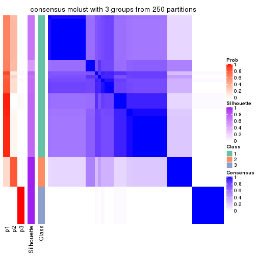
consensus_heatmap(res, k = 4)
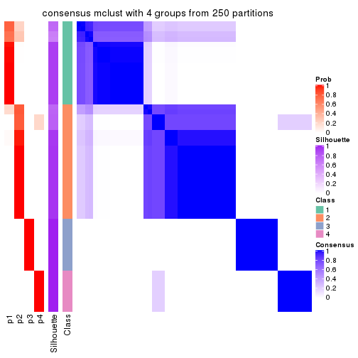
consensus_heatmap(res, k = 5)
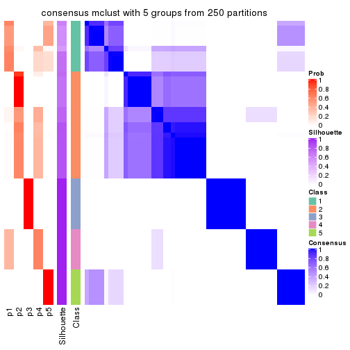
consensus_heatmap(res, k = 6)
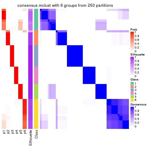
Heatmaps for the membership of samples in all partitions to see how consistent they are:
membership_heatmap(res, k = 2)
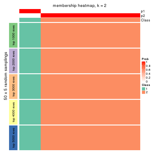
membership_heatmap(res, k = 3)
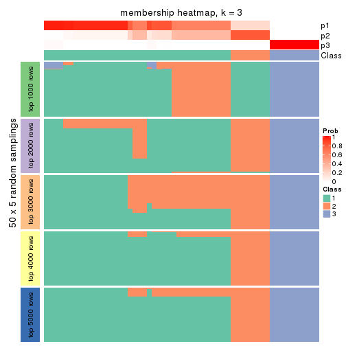
membership_heatmap(res, k = 4)
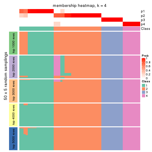
membership_heatmap(res, k = 5)
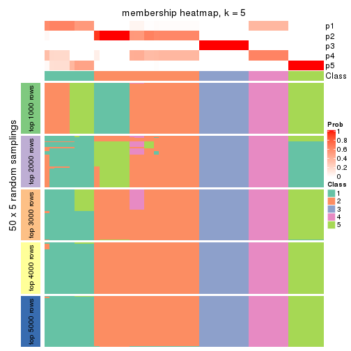
membership_heatmap(res, k = 6)
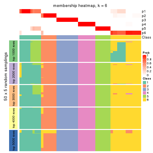
As soon as we have had the classes for columns, we can look for signatures which are significantly different between classes which can be candidate marks for certain classes. Following are the heatmaps for signatures.
Signature heatmaps where rows are scaled:
get_signatures(res, k = 2)
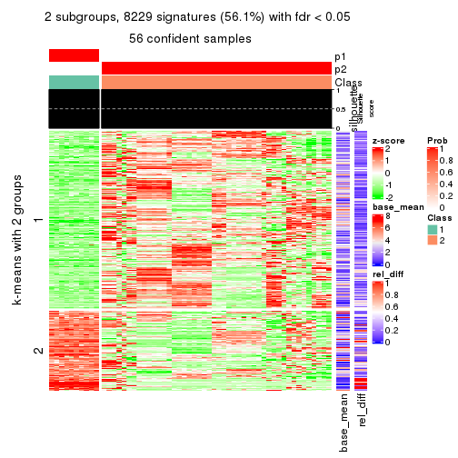
get_signatures(res, k = 3)
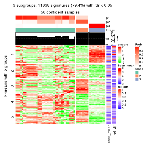
get_signatures(res, k = 4)
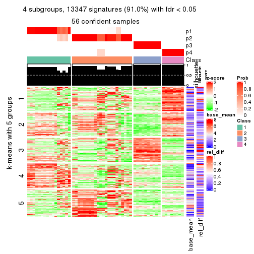
get_signatures(res, k = 5)
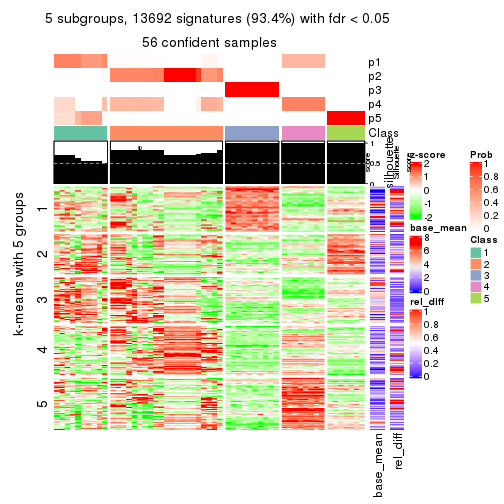
get_signatures(res, k = 6)
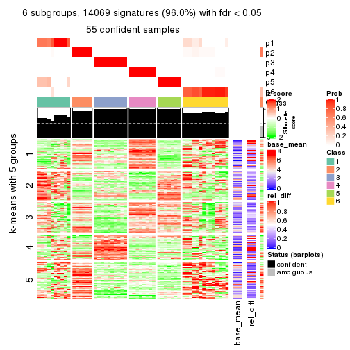
Signature heatmaps where rows are not scaled:
get_signatures(res, k = 2, scale_rows = FALSE)

get_signatures(res, k = 3, scale_rows = FALSE)
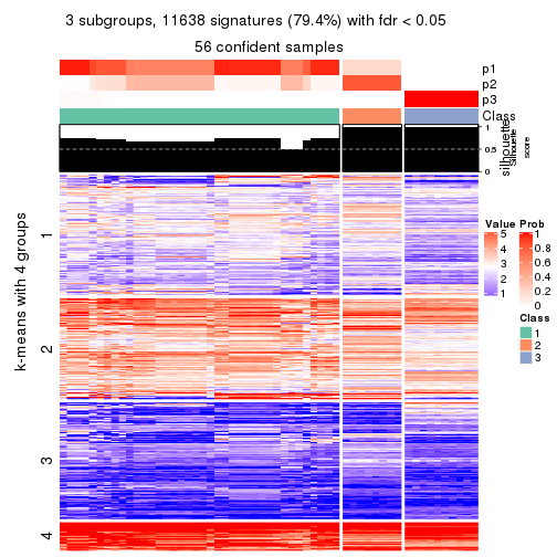
get_signatures(res, k = 4, scale_rows = FALSE)
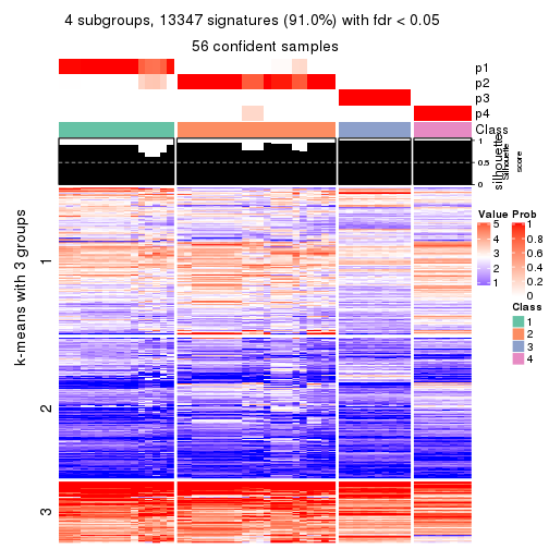
get_signatures(res, k = 5, scale_rows = FALSE)
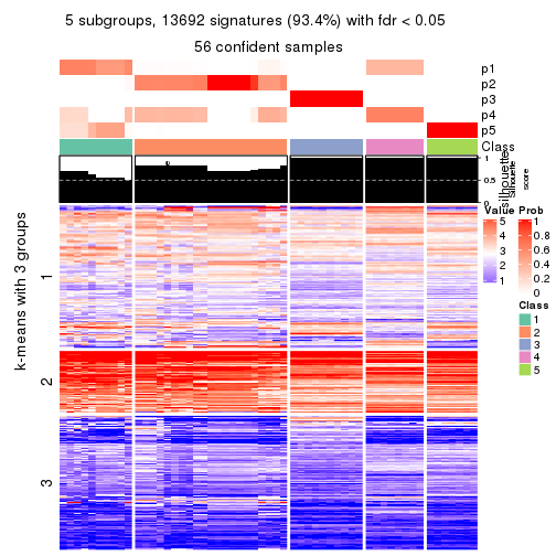
get_signatures(res, k = 6, scale_rows = FALSE)
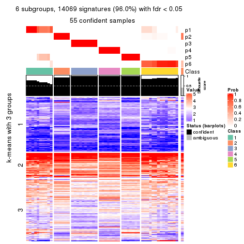
Compare the overlap of signatures from different k:
compare_signatures(res)
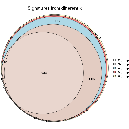
get_signature() returns a data frame invisibly. TO get the list of signatures, the function
call should be assigned to a variable explicitly. In following code, if plot argument is set
to FALSE, no heatmap is plotted while only the differential analysis is performed.
# code only for demonstration
tb = get_signature(res, k = ..., plot = FALSE)
An example of the output of tb is:
#> which_row fdr mean_1 mean_2 scaled_mean_1 scaled_mean_2 km
#> 1 38 0.042760348 8.373488 9.131774 -0.5533452 0.5164555 1
#> 2 40 0.018707592 7.106213 8.469186 -0.6173731 0.5762149 1
#> 3 55 0.019134737 10.221463 11.207825 -0.6159697 0.5749050 1
#> 4 59 0.006059896 5.921854 7.869574 -0.6899429 0.6439467 1
#> 5 60 0.018055526 8.928898 10.211722 -0.6204761 0.5791110 1
#> 6 98 0.009384629 15.714769 14.887706 0.6635654 -0.6193277 2
...
The columns in tb are:
which_row: row indices corresponding to the input matrix.fdr: FDR for the differential test. mean_x: The mean value in group x.scaled_mean_x: The mean value in group x after rows are scaled.km: Row groups if k-means clustering is applied to rows.UMAP plot which shows how samples are separated.
dimension_reduction(res, k = 2, method = "UMAP")
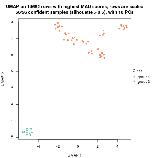
dimension_reduction(res, k = 3, method = "UMAP")

dimension_reduction(res, k = 4, method = "UMAP")
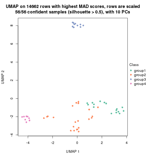
dimension_reduction(res, k = 5, method = "UMAP")
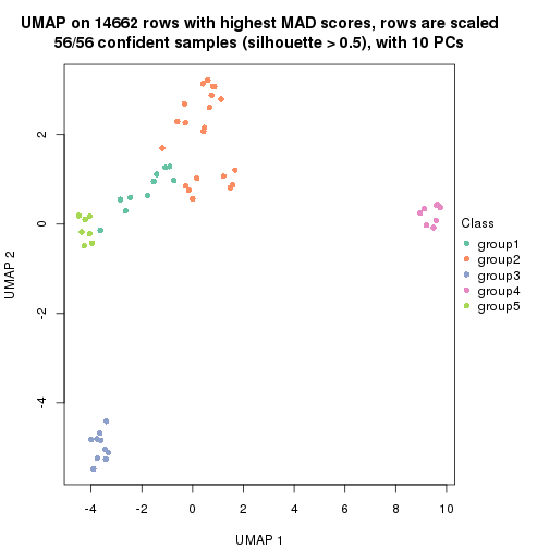
dimension_reduction(res, k = 6, method = "UMAP")
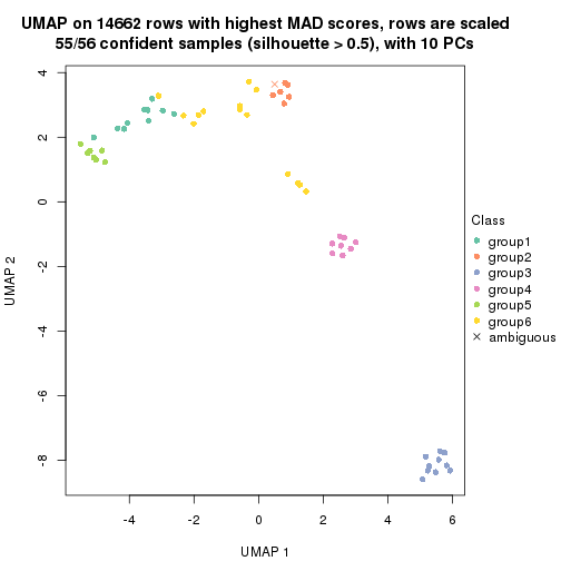
Following heatmap shows how subgroups are split when increasing k:
collect_classes(res)
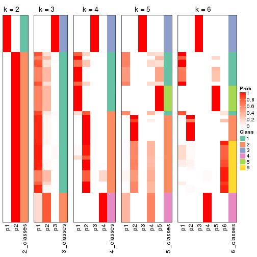
If matrix rows can be associated to genes, consider to use functional_enrichment(res,
...) to perform function enrichment for the signature genes. See this vignette for more detailed explanations.
The object with results only for a single top-value method and a single partition method can be extracted as:
res = res_list["MAD", "NMF"]
# you can also extract it by
# res = res_list["MAD:NMF"]
A summary of res and all the functions that can be applied to it:
res
#> A 'ConsensusPartition' object with k = 2, 3, 4, 5, 6.
#> On a matrix with 14662 rows and 56 columns.
#> Top rows (1000, 2000, 3000, 4000, 5000) are extracted by 'MAD' method.
#> Subgroups are detected by 'NMF' method.
#> Performed in total 1250 partitions by row resampling.
#> Best k for subgroups seems to be 5.
#>
#> Following methods can be applied to this 'ConsensusPartition' object:
#> [1] "cola_report" "collect_classes" "collect_plots"
#> [4] "collect_stats" "colnames" "compare_signatures"
#> [7] "consensus_heatmap" "dimension_reduction" "functional_enrichment"
#> [10] "get_anno_col" "get_anno" "get_classes"
#> [13] "get_consensus" "get_matrix" "get_membership"
#> [16] "get_param" "get_signatures" "get_stats"
#> [19] "is_best_k" "is_stable_k" "membership_heatmap"
#> [22] "ncol" "nrow" "plot_ecdf"
#> [25] "rownames" "select_partition_number" "show"
#> [28] "suggest_best_k" "test_to_known_factors"
collect_plots() function collects all the plots made from res for all k (number of partitions)
into one single page to provide an easy and fast comparison between different k.
collect_plots(res)
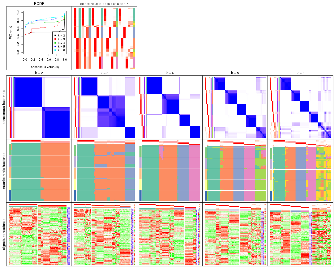
The plots are:
k and the heatmap of
predicted classes for each k.k.k.k.All the plots in panels can be made by individual functions and they are plotted later in this section.
select_partition_number() produces several plots showing different
statistics for choosing “optimized” k. There are following statistics:
k;k, the area increased is defined as \(A_k - A_{k-1}\).The detailed explanations of these statistics can be found in the cola vignette.
Generally speaking, lower PAC score, higher mean silhouette score or higher
concordance corresponds to better partition. Rand index and Jaccard index
measure how similar the current partition is compared to partition with k-1.
If they are too similar, we won't accept k is better than k-1.
select_partition_number(res)
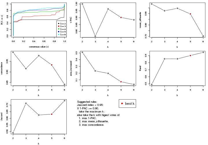
The numeric values for all these statistics can be obtained by get_stats().
get_stats(res)
#> k 1-PAC mean_silhouette concordance area_increased Rand Jaccard
#> 2 2 1.000 0.984 0.992 0.5090 0.491 0.491
#> 3 3 0.766 0.925 0.916 0.2340 0.854 0.713
#> 4 4 0.964 0.946 0.977 0.1965 0.855 0.625
#> 5 5 0.902 0.897 0.933 0.0723 0.901 0.631
#> 6 6 0.885 0.702 0.841 0.0324 0.947 0.733
suggest_best_k() suggests the best \(k\) based on these statistics. The rules are as follows:
suggest_best_k(res)
#> [1] 5
#> attr(,"optional")
#> [1] 2 4
There is also optional best \(k\) = 2 4 that is worth to check.
Following shows the table of the partitions (You need to click the show/hide
code output link to see it). The membership matrix (columns with name p*)
is inferred by
clue::cl_consensus()
function with the SE method. Basically the value in the membership matrix
represents the probability to belong to a certain group. The finall class
label for an item is determined with the group with highest probability it
belongs to.
In get_classes() function, the entropy is calculated from the membership
matrix and the silhouette score is calculated from the consensus matrix.
cbind(get_classes(res, k = 2), get_membership(res, k = 2))
#> class entropy silhouette p1 p2
#> SRR073723 1 0.000 0.995 1.000 0.000
#> SRR073724 1 0.000 0.995 1.000 0.000
#> SRR073725 1 0.000 0.995 1.000 0.000
#> SRR073726 2 0.000 0.989 0.000 1.000
#> SRR073727 1 0.000 0.995 1.000 0.000
#> SRR073728 2 0.469 0.895 0.100 0.900
#> SRR073729 2 0.388 0.920 0.076 0.924
#> SRR073730 2 0.529 0.871 0.120 0.880
#> SRR073731 2 0.000 0.989 0.000 1.000
#> SRR073732 2 0.000 0.989 0.000 1.000
#> SRR073733 2 0.000 0.989 0.000 1.000
#> SRR073734 2 0.000 0.989 0.000 1.000
#> SRR073735 2 0.000 0.989 0.000 1.000
#> SRR073736 2 0.000 0.989 0.000 1.000
#> SRR073737 2 0.000 0.989 0.000 1.000
#> SRR073738 1 0.000 0.995 1.000 0.000
#> SRR073739 1 0.000 0.995 1.000 0.000
#> SRR073740 1 0.000 0.995 1.000 0.000
#> SRR073741 1 0.000 0.995 1.000 0.000
#> SRR073742 1 0.000 0.995 1.000 0.000
#> SRR073743 1 0.000 0.995 1.000 0.000
#> SRR073744 1 0.000 0.995 1.000 0.000
#> SRR073745 1 0.000 0.995 1.000 0.000
#> SRR073746 1 0.000 0.995 1.000 0.000
#> SRR073747 1 0.000 0.995 1.000 0.000
#> SRR073748 1 0.000 0.995 1.000 0.000
#> SRR073749 1 0.000 0.995 1.000 0.000
#> SRR073750 1 0.000 0.995 1.000 0.000
#> SRR073751 1 0.584 0.834 0.860 0.140
#> SRR073752 2 0.000 0.989 0.000 1.000
#> SRR073753 2 0.000 0.989 0.000 1.000
#> SRR073754 2 0.000 0.989 0.000 1.000
#> SRR073755 2 0.000 0.989 0.000 1.000
#> SRR073756 2 0.000 0.989 0.000 1.000
#> SRR073758 2 0.000 0.989 0.000 1.000
#> SRR073759 2 0.000 0.989 0.000 1.000
#> SRR073760 2 0.000 0.989 0.000 1.000
#> SRR073761 2 0.000 0.989 0.000 1.000
#> SRR073763 2 0.000 0.989 0.000 1.000
#> SRR073764 2 0.000 0.989 0.000 1.000
#> SRR073765 2 0.000 0.989 0.000 1.000
#> SRR073766 2 0.000 0.989 0.000 1.000
#> SRR073767 2 0.000 0.989 0.000 1.000
#> SRR073768 2 0.000 0.989 0.000 1.000
#> SRR073769 1 0.000 0.995 1.000 0.000
#> SRR073770 1 0.000 0.995 1.000 0.000
#> SRR073771 1 0.000 0.995 1.000 0.000
#> SRR073772 1 0.000 0.995 1.000 0.000
#> SRR073773 1 0.000 0.995 1.000 0.000
#> SRR073774 1 0.000 0.995 1.000 0.000
#> SRR073775 1 0.000 0.995 1.000 0.000
#> SRR073776 1 0.000 0.995 1.000 0.000
#> SRR073777 1 0.000 0.995 1.000 0.000
#> SRR073778 1 0.000 0.995 1.000 0.000
#> SRR073779 2 0.000 0.989 0.000 1.000
#> SRR073780 2 0.000 0.989 0.000 1.000
cbind(get_classes(res, k = 3), get_membership(res, k = 3))
#> class entropy silhouette p1 p2 p3
#> SRR073723 1 0.4291 0.725 0.820 0.000 0.180
#> SRR073724 1 0.0000 0.986 1.000 0.000 0.000
#> SRR073725 1 0.0000 0.986 1.000 0.000 0.000
#> SRR073726 2 0.2448 0.908 0.000 0.924 0.076
#> SRR073727 1 0.0000 0.986 1.000 0.000 0.000
#> SRR073728 2 0.2796 0.849 0.092 0.908 0.000
#> SRR073729 2 0.2945 0.850 0.088 0.908 0.004
#> SRR073730 2 0.2878 0.845 0.096 0.904 0.000
#> SRR073731 2 0.0237 0.905 0.004 0.996 0.000
#> SRR073732 2 0.0000 0.906 0.000 1.000 0.000
#> SRR073733 2 0.0000 0.906 0.000 1.000 0.000
#> SRR073734 2 0.0237 0.905 0.004 0.996 0.000
#> SRR073735 2 0.0000 0.906 0.000 1.000 0.000
#> SRR073736 2 0.0000 0.906 0.000 1.000 0.000
#> SRR073737 2 0.0237 0.905 0.004 0.996 0.000
#> SRR073738 1 0.0000 0.986 1.000 0.000 0.000
#> SRR073739 1 0.0000 0.986 1.000 0.000 0.000
#> SRR073740 1 0.0000 0.986 1.000 0.000 0.000
#> SRR073741 1 0.0000 0.986 1.000 0.000 0.000
#> SRR073742 1 0.0000 0.986 1.000 0.000 0.000
#> SRR073743 1 0.0000 0.986 1.000 0.000 0.000
#> SRR073744 1 0.0000 0.986 1.000 0.000 0.000
#> SRR073745 1 0.0000 0.986 1.000 0.000 0.000
#> SRR073746 1 0.0000 0.986 1.000 0.000 0.000
#> SRR073747 1 0.0000 0.986 1.000 0.000 0.000
#> SRR073748 1 0.0000 0.986 1.000 0.000 0.000
#> SRR073749 1 0.0000 0.986 1.000 0.000 0.000
#> SRR073750 1 0.0000 0.986 1.000 0.000 0.000
#> SRR073751 2 0.8414 0.218 0.380 0.528 0.092
#> SRR073752 2 0.0747 0.900 0.016 0.984 0.000
#> SRR073753 2 0.0424 0.904 0.008 0.992 0.000
#> SRR073754 2 0.1860 0.909 0.000 0.948 0.052
#> SRR073755 2 0.4121 0.895 0.000 0.832 0.168
#> SRR073756 2 0.4121 0.895 0.000 0.832 0.168
#> SRR073758 2 0.4121 0.895 0.000 0.832 0.168
#> SRR073759 2 0.0000 0.906 0.000 1.000 0.000
#> SRR073760 2 0.4121 0.895 0.000 0.832 0.168
#> SRR073761 2 0.4121 0.895 0.000 0.832 0.168
#> SRR073763 2 0.4121 0.895 0.000 0.832 0.168
#> SRR073764 2 0.4121 0.895 0.000 0.832 0.168
#> SRR073765 2 0.4121 0.895 0.000 0.832 0.168
#> SRR073766 2 0.4121 0.895 0.000 0.832 0.168
#> SRR073767 2 0.4121 0.895 0.000 0.832 0.168
#> SRR073768 2 0.4121 0.895 0.000 0.832 0.168
#> SRR073769 3 0.4121 1.000 0.168 0.000 0.832
#> SRR073770 3 0.4121 1.000 0.168 0.000 0.832
#> SRR073771 3 0.4121 1.000 0.168 0.000 0.832
#> SRR073772 3 0.4121 1.000 0.168 0.000 0.832
#> SRR073773 3 0.4121 1.000 0.168 0.000 0.832
#> SRR073774 3 0.4121 1.000 0.168 0.000 0.832
#> SRR073775 3 0.4121 1.000 0.168 0.000 0.832
#> SRR073776 3 0.4121 1.000 0.168 0.000 0.832
#> SRR073777 3 0.4121 1.000 0.168 0.000 0.832
#> SRR073778 3 0.4121 1.000 0.168 0.000 0.832
#> SRR073779 2 0.1529 0.909 0.000 0.960 0.040
#> SRR073780 2 0.2356 0.908 0.000 0.928 0.072
cbind(get_classes(res, k = 4), get_membership(res, k = 4))
#> class entropy silhouette p1 p2 p3 p4
#> SRR073723 3 0.517 0.0561 0.484 0.004 0.512 0.000
#> SRR073724 1 0.000 1.0000 1.000 0.000 0.000 0.000
#> SRR073725 1 0.000 1.0000 1.000 0.000 0.000 0.000
#> SRR073726 2 0.401 0.7325 0.000 0.756 0.000 0.244
#> SRR073727 1 0.000 1.0000 1.000 0.000 0.000 0.000
#> SRR073728 2 0.000 0.9511 0.000 1.000 0.000 0.000
#> SRR073729 2 0.000 0.9511 0.000 1.000 0.000 0.000
#> SRR073730 2 0.000 0.9511 0.000 1.000 0.000 0.000
#> SRR073731 2 0.000 0.9511 0.000 1.000 0.000 0.000
#> SRR073732 2 0.000 0.9511 0.000 1.000 0.000 0.000
#> SRR073733 2 0.000 0.9511 0.000 1.000 0.000 0.000
#> SRR073734 2 0.000 0.9511 0.000 1.000 0.000 0.000
#> SRR073735 2 0.000 0.9511 0.000 1.000 0.000 0.000
#> SRR073736 2 0.000 0.9511 0.000 1.000 0.000 0.000
#> SRR073737 2 0.000 0.9511 0.000 1.000 0.000 0.000
#> SRR073738 1 0.000 1.0000 1.000 0.000 0.000 0.000
#> SRR073739 1 0.000 1.0000 1.000 0.000 0.000 0.000
#> SRR073740 1 0.000 1.0000 1.000 0.000 0.000 0.000
#> SRR073741 1 0.000 1.0000 1.000 0.000 0.000 0.000
#> SRR073742 1 0.000 1.0000 1.000 0.000 0.000 0.000
#> SRR073743 1 0.000 1.0000 1.000 0.000 0.000 0.000
#> SRR073744 1 0.000 1.0000 1.000 0.000 0.000 0.000
#> SRR073745 1 0.000 1.0000 1.000 0.000 0.000 0.000
#> SRR073746 1 0.000 1.0000 1.000 0.000 0.000 0.000
#> SRR073747 1 0.000 1.0000 1.000 0.000 0.000 0.000
#> SRR073748 1 0.000 1.0000 1.000 0.000 0.000 0.000
#> SRR073749 1 0.000 1.0000 1.000 0.000 0.000 0.000
#> SRR073750 1 0.000 1.0000 1.000 0.000 0.000 0.000
#> SRR073751 2 0.187 0.9014 0.000 0.928 0.072 0.000
#> SRR073752 2 0.000 0.9511 0.000 1.000 0.000 0.000
#> SRR073753 2 0.000 0.9511 0.000 1.000 0.000 0.000
#> SRR073754 2 0.312 0.8389 0.000 0.844 0.000 0.156
#> SRR073755 4 0.000 1.0000 0.000 0.000 0.000 1.000
#> SRR073756 4 0.000 1.0000 0.000 0.000 0.000 1.000
#> SRR073758 4 0.000 1.0000 0.000 0.000 0.000 1.000
#> SRR073759 2 0.000 0.9511 0.000 1.000 0.000 0.000
#> SRR073760 4 0.000 1.0000 0.000 0.000 0.000 1.000
#> SRR073761 4 0.000 1.0000 0.000 0.000 0.000 1.000
#> SRR073763 4 0.000 1.0000 0.000 0.000 0.000 1.000
#> SRR073764 4 0.000 1.0000 0.000 0.000 0.000 1.000
#> SRR073765 4 0.000 1.0000 0.000 0.000 0.000 1.000
#> SRR073766 4 0.000 1.0000 0.000 0.000 0.000 1.000
#> SRR073767 4 0.000 1.0000 0.000 0.000 0.000 1.000
#> SRR073768 4 0.000 1.0000 0.000 0.000 0.000 1.000
#> SRR073769 3 0.000 0.9455 0.000 0.000 1.000 0.000
#> SRR073770 3 0.000 0.9455 0.000 0.000 1.000 0.000
#> SRR073771 3 0.000 0.9455 0.000 0.000 1.000 0.000
#> SRR073772 3 0.000 0.9455 0.000 0.000 1.000 0.000
#> SRR073773 3 0.000 0.9455 0.000 0.000 1.000 0.000
#> SRR073774 3 0.000 0.9455 0.000 0.000 1.000 0.000
#> SRR073775 3 0.000 0.9455 0.000 0.000 1.000 0.000
#> SRR073776 3 0.000 0.9455 0.000 0.000 1.000 0.000
#> SRR073777 3 0.000 0.9455 0.000 0.000 1.000 0.000
#> SRR073778 3 0.000 0.9455 0.000 0.000 1.000 0.000
#> SRR073779 2 0.292 0.8538 0.000 0.860 0.000 0.140
#> SRR073780 2 0.373 0.7763 0.000 0.788 0.000 0.212
cbind(get_classes(res, k = 5), get_membership(res, k = 5))
#> class entropy silhouette p1 p2 p3 p4 p5
#> SRR073723 5 0.1857 0.7773 0.060 0.008 0.004 0.000 0.928
#> SRR073724 5 0.3424 0.7479 0.240 0.000 0.000 0.000 0.760
#> SRR073725 1 0.4227 0.0571 0.580 0.000 0.000 0.000 0.420
#> SRR073726 5 0.4676 0.7386 0.000 0.072 0.000 0.208 0.720
#> SRR073727 5 0.3424 0.7471 0.240 0.000 0.000 0.000 0.760
#> SRR073728 2 0.3819 0.7714 0.000 0.756 0.016 0.000 0.228
#> SRR073729 2 0.3696 0.7863 0.000 0.772 0.016 0.000 0.212
#> SRR073730 2 0.4329 0.6598 0.000 0.672 0.016 0.000 0.312
#> SRR073731 2 0.0000 0.9326 0.000 1.000 0.000 0.000 0.000
#> SRR073732 2 0.0404 0.9268 0.000 0.988 0.000 0.000 0.012
#> SRR073733 2 0.0000 0.9326 0.000 1.000 0.000 0.000 0.000
#> SRR073734 2 0.0000 0.9326 0.000 1.000 0.000 0.000 0.000
#> SRR073735 2 0.0000 0.9326 0.000 1.000 0.000 0.000 0.000
#> SRR073736 2 0.0000 0.9326 0.000 1.000 0.000 0.000 0.000
#> SRR073737 2 0.0000 0.9326 0.000 1.000 0.000 0.000 0.000
#> SRR073738 5 0.3424 0.7479 0.240 0.000 0.000 0.000 0.760
#> SRR073739 1 0.0000 0.9448 1.000 0.000 0.000 0.000 0.000
#> SRR073740 1 0.0000 0.9448 1.000 0.000 0.000 0.000 0.000
#> SRR073741 1 0.0000 0.9448 1.000 0.000 0.000 0.000 0.000
#> SRR073742 1 0.0000 0.9448 1.000 0.000 0.000 0.000 0.000
#> SRR073743 1 0.0000 0.9448 1.000 0.000 0.000 0.000 0.000
#> SRR073744 1 0.0000 0.9448 1.000 0.000 0.000 0.000 0.000
#> SRR073745 1 0.0000 0.9448 1.000 0.000 0.000 0.000 0.000
#> SRR073746 1 0.0963 0.9235 0.964 0.000 0.000 0.000 0.036
#> SRR073747 1 0.0609 0.9370 0.980 0.000 0.000 0.000 0.020
#> SRR073748 1 0.0609 0.9370 0.980 0.000 0.000 0.000 0.020
#> SRR073749 1 0.0609 0.9370 0.980 0.000 0.000 0.000 0.020
#> SRR073750 5 0.3774 0.6765 0.296 0.000 0.000 0.000 0.704
#> SRR073751 5 0.2640 0.7578 0.016 0.052 0.032 0.000 0.900
#> SRR073752 2 0.0162 0.9308 0.000 0.996 0.000 0.000 0.004
#> SRR073753 2 0.0000 0.9326 0.000 1.000 0.000 0.000 0.000
#> SRR073754 5 0.4059 0.7664 0.000 0.052 0.000 0.172 0.776
#> SRR073755 4 0.0771 0.9802 0.000 0.004 0.000 0.976 0.020
#> SRR073756 4 0.0510 0.9850 0.000 0.000 0.000 0.984 0.016
#> SRR073758 4 0.1121 0.9581 0.000 0.000 0.000 0.956 0.044
#> SRR073759 2 0.1121 0.9043 0.000 0.956 0.000 0.000 0.044
#> SRR073760 4 0.0000 0.9925 0.000 0.000 0.000 1.000 0.000
#> SRR073761 4 0.0000 0.9925 0.000 0.000 0.000 1.000 0.000
#> SRR073763 4 0.0000 0.9925 0.000 0.000 0.000 1.000 0.000
#> SRR073764 4 0.0000 0.9925 0.000 0.000 0.000 1.000 0.000
#> SRR073765 4 0.0000 0.9925 0.000 0.000 0.000 1.000 0.000
#> SRR073766 4 0.0000 0.9925 0.000 0.000 0.000 1.000 0.000
#> SRR073767 4 0.0000 0.9925 0.000 0.000 0.000 1.000 0.000
#> SRR073768 4 0.0000 0.9925 0.000 0.000 0.000 1.000 0.000
#> SRR073769 3 0.0000 1.0000 0.000 0.000 1.000 0.000 0.000
#> SRR073770 3 0.0000 1.0000 0.000 0.000 1.000 0.000 0.000
#> SRR073771 3 0.0000 1.0000 0.000 0.000 1.000 0.000 0.000
#> SRR073772 3 0.0000 1.0000 0.000 0.000 1.000 0.000 0.000
#> SRR073773 3 0.0000 1.0000 0.000 0.000 1.000 0.000 0.000
#> SRR073774 3 0.0000 1.0000 0.000 0.000 1.000 0.000 0.000
#> SRR073775 3 0.0000 1.0000 0.000 0.000 1.000 0.000 0.000
#> SRR073776 3 0.0000 1.0000 0.000 0.000 1.000 0.000 0.000
#> SRR073777 3 0.0000 1.0000 0.000 0.000 1.000 0.000 0.000
#> SRR073778 3 0.0000 1.0000 0.000 0.000 1.000 0.000 0.000
#> SRR073779 5 0.4624 0.7483 0.000 0.164 0.000 0.096 0.740
#> SRR073780 5 0.4637 0.7486 0.000 0.076 0.000 0.196 0.728
cbind(get_classes(res, k = 6), get_membership(res, k = 6))
#> class entropy silhouette p1 p2 p3 p4 p5 p6
#> SRR073723 5 0.2841 0.20138 0.032 0.000 0.012 0.000 0.864 0.092
#> SRR073724 6 0.5784 0.19117 0.176 0.000 0.000 0.000 0.404 0.420
#> SRR073725 1 0.5480 0.08736 0.528 0.000 0.000 0.000 0.328 0.144
#> SRR073726 6 0.4160 0.37564 0.000 0.052 0.000 0.076 0.084 0.788
#> SRR073727 6 0.5479 0.30533 0.128 0.000 0.000 0.000 0.388 0.484
#> SRR073728 5 0.4973 0.36546 0.004 0.300 0.036 0.020 0.636 0.004
#> SRR073729 5 0.4917 0.35576 0.000 0.304 0.040 0.020 0.632 0.004
#> SRR073730 5 0.4939 0.37529 0.004 0.292 0.036 0.020 0.644 0.004
#> SRR073731 2 0.0000 0.91473 0.000 1.000 0.000 0.000 0.000 0.000
#> SRR073732 2 0.0260 0.91157 0.000 0.992 0.000 0.000 0.000 0.008
#> SRR073733 2 0.0000 0.91473 0.000 1.000 0.000 0.000 0.000 0.000
#> SRR073734 2 0.0000 0.91473 0.000 1.000 0.000 0.000 0.000 0.000
#> SRR073735 2 0.0000 0.91473 0.000 1.000 0.000 0.000 0.000 0.000
#> SRR073736 2 0.0000 0.91473 0.000 1.000 0.000 0.000 0.000 0.000
#> SRR073737 2 0.0000 0.91473 0.000 1.000 0.000 0.000 0.000 0.000
#> SRR073738 5 0.5782 -0.37834 0.176 0.000 0.000 0.000 0.424 0.400
#> SRR073739 1 0.0000 0.93530 1.000 0.000 0.000 0.000 0.000 0.000
#> SRR073740 1 0.0000 0.93530 1.000 0.000 0.000 0.000 0.000 0.000
#> SRR073741 1 0.0146 0.93468 0.996 0.000 0.000 0.000 0.004 0.000
#> SRR073742 1 0.0146 0.93468 0.996 0.000 0.000 0.000 0.004 0.000
#> SRR073743 1 0.0000 0.93530 1.000 0.000 0.000 0.000 0.000 0.000
#> SRR073744 1 0.0146 0.93468 0.996 0.000 0.000 0.000 0.004 0.000
#> SRR073745 1 0.0146 0.93469 0.996 0.000 0.000 0.000 0.000 0.004
#> SRR073746 1 0.1082 0.90129 0.956 0.000 0.000 0.000 0.004 0.040
#> SRR073747 1 0.0717 0.92678 0.976 0.000 0.000 0.000 0.016 0.008
#> SRR073748 1 0.0806 0.92451 0.972 0.000 0.000 0.000 0.020 0.008
#> SRR073749 1 0.0806 0.92451 0.972 0.000 0.000 0.000 0.020 0.008
#> SRR073750 5 0.6074 -0.29388 0.268 0.000 0.000 0.000 0.376 0.356
#> SRR073751 5 0.4175 -0.00305 0.004 0.008 0.032 0.000 0.720 0.236
#> SRR073752 2 0.2053 0.85013 0.000 0.888 0.000 0.000 0.004 0.108
#> SRR073753 2 0.2070 0.85826 0.000 0.896 0.000 0.000 0.012 0.092
#> SRR073754 6 0.5319 0.42608 0.000 0.048 0.000 0.028 0.408 0.516
#> SRR073755 4 0.4192 0.47150 0.000 0.016 0.000 0.572 0.000 0.412
#> SRR073756 4 0.4051 0.44621 0.000 0.008 0.000 0.560 0.000 0.432
#> SRR073758 6 0.4097 -0.45826 0.000 0.008 0.000 0.492 0.000 0.500
#> SRR073759 2 0.3982 0.38688 0.000 0.536 0.000 0.000 0.004 0.460
#> SRR073760 4 0.0000 0.89890 0.000 0.000 0.000 1.000 0.000 0.000
#> SRR073761 4 0.0000 0.89890 0.000 0.000 0.000 1.000 0.000 0.000
#> SRR073763 4 0.0000 0.89890 0.000 0.000 0.000 1.000 0.000 0.000
#> SRR073764 4 0.0000 0.89890 0.000 0.000 0.000 1.000 0.000 0.000
#> SRR073765 4 0.0000 0.89890 0.000 0.000 0.000 1.000 0.000 0.000
#> SRR073766 4 0.0000 0.89890 0.000 0.000 0.000 1.000 0.000 0.000
#> SRR073767 4 0.0000 0.89890 0.000 0.000 0.000 1.000 0.000 0.000
#> SRR073768 4 0.0000 0.89890 0.000 0.000 0.000 1.000 0.000 0.000
#> SRR073769 3 0.0000 1.00000 0.000 0.000 1.000 0.000 0.000 0.000
#> SRR073770 3 0.0000 1.00000 0.000 0.000 1.000 0.000 0.000 0.000
#> SRR073771 3 0.0000 1.00000 0.000 0.000 1.000 0.000 0.000 0.000
#> SRR073772 3 0.0000 1.00000 0.000 0.000 1.000 0.000 0.000 0.000
#> SRR073773 3 0.0000 1.00000 0.000 0.000 1.000 0.000 0.000 0.000
#> SRR073774 3 0.0000 1.00000 0.000 0.000 1.000 0.000 0.000 0.000
#> SRR073775 3 0.0000 1.00000 0.000 0.000 1.000 0.000 0.000 0.000
#> SRR073776 3 0.0000 1.00000 0.000 0.000 1.000 0.000 0.000 0.000
#> SRR073777 3 0.0000 1.00000 0.000 0.000 1.000 0.000 0.000 0.000
#> SRR073778 3 0.0000 1.00000 0.000 0.000 1.000 0.000 0.000 0.000
#> SRR073779 6 0.5509 0.47504 0.000 0.064 0.000 0.036 0.340 0.560
#> SRR073780 6 0.5478 0.48609 0.000 0.052 0.000 0.060 0.280 0.608
Heatmaps for the consensus matrix. It visualizes the probability of two samples to be in a same group.
consensus_heatmap(res, k = 2)
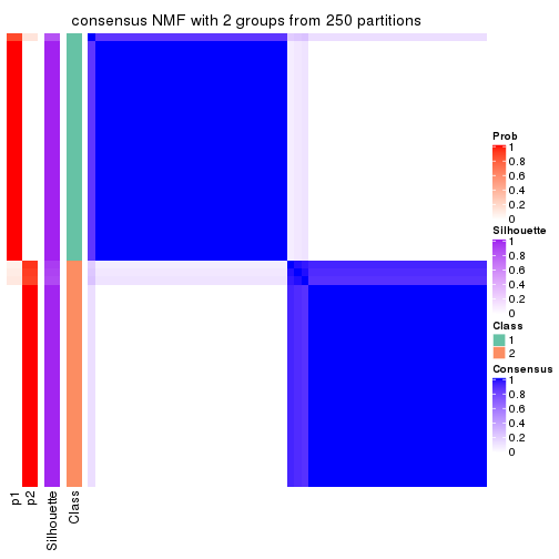
consensus_heatmap(res, k = 3)
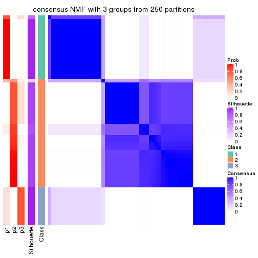
consensus_heatmap(res, k = 4)
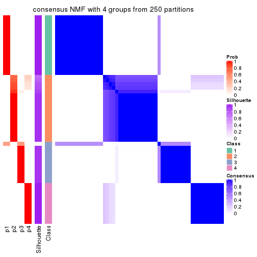
consensus_heatmap(res, k = 5)
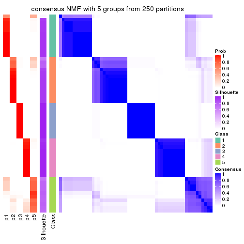
consensus_heatmap(res, k = 6)
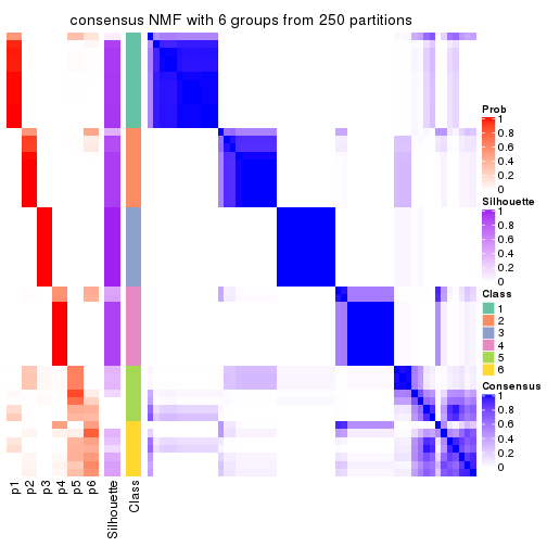
Heatmaps for the membership of samples in all partitions to see how consistent they are:
membership_heatmap(res, k = 2)
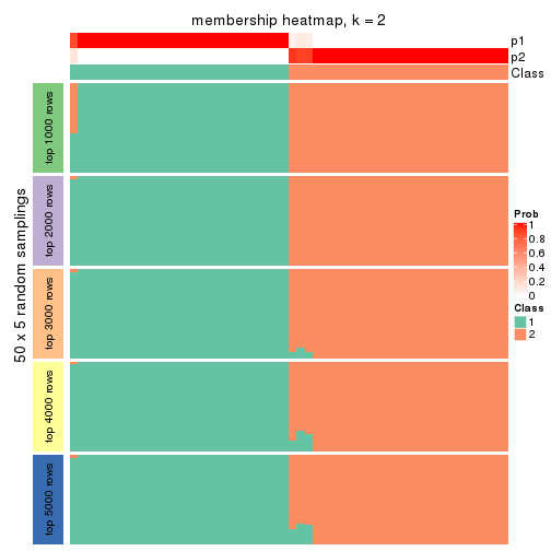
membership_heatmap(res, k = 3)
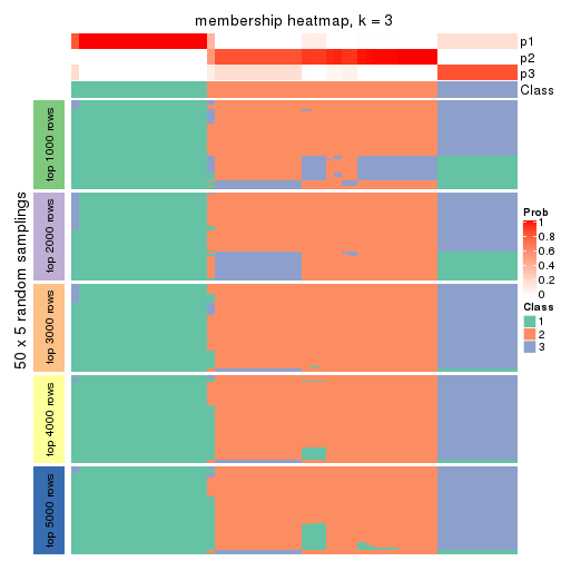
membership_heatmap(res, k = 4)

membership_heatmap(res, k = 5)
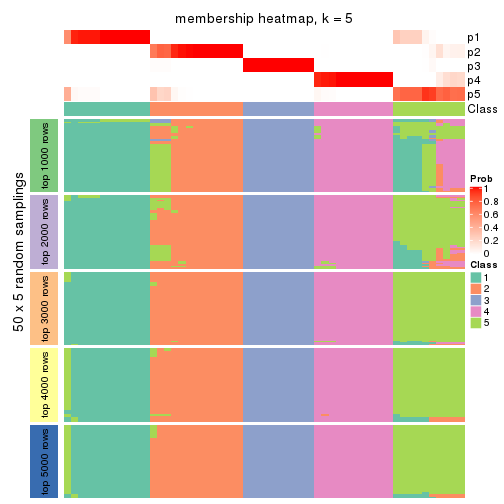
membership_heatmap(res, k = 6)
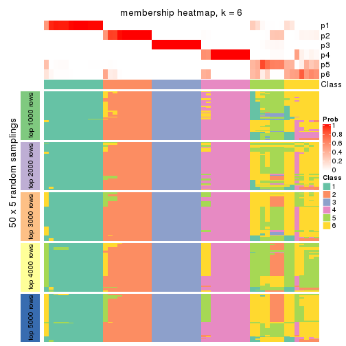
As soon as we have had the classes for columns, we can look for signatures which are significantly different between classes which can be candidate marks for certain classes. Following are the heatmaps for signatures.
Signature heatmaps where rows are scaled:
get_signatures(res, k = 2)
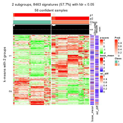
get_signatures(res, k = 3)
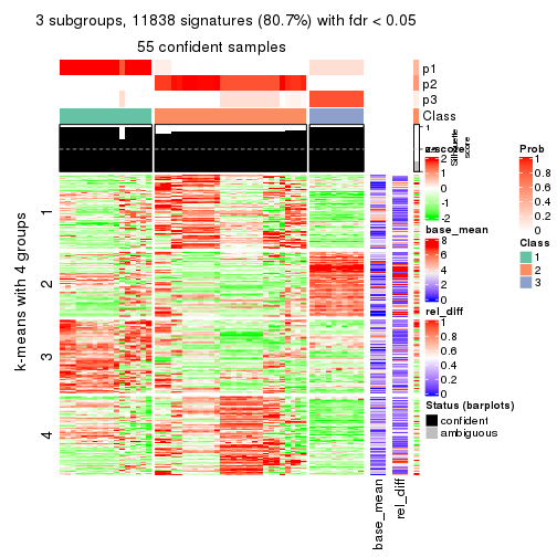
get_signatures(res, k = 4)
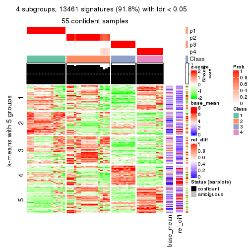
get_signatures(res, k = 5)
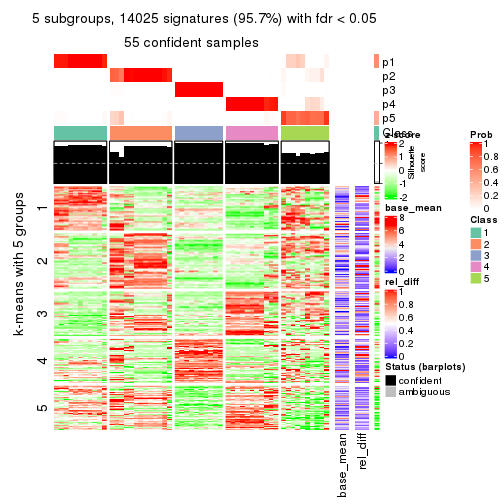
get_signatures(res, k = 6)
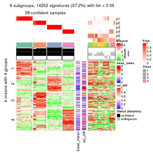
Signature heatmaps where rows are not scaled:
get_signatures(res, k = 2, scale_rows = FALSE)

get_signatures(res, k = 3, scale_rows = FALSE)
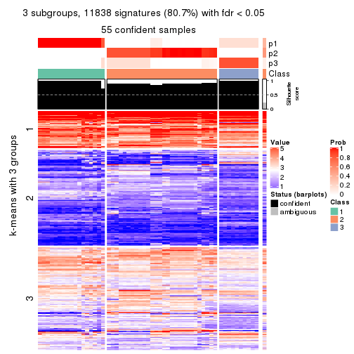
get_signatures(res, k = 4, scale_rows = FALSE)
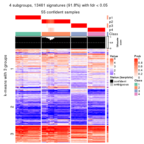
get_signatures(res, k = 5, scale_rows = FALSE)
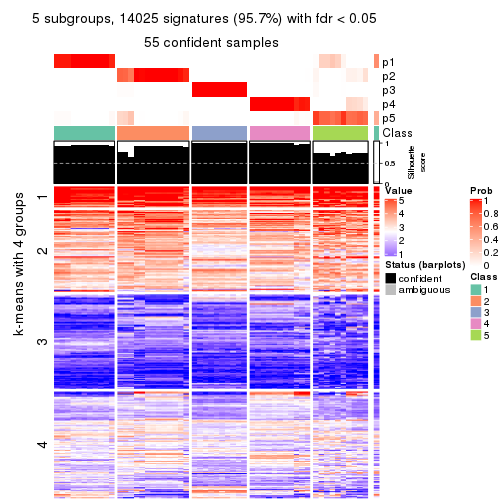
get_signatures(res, k = 6, scale_rows = FALSE)
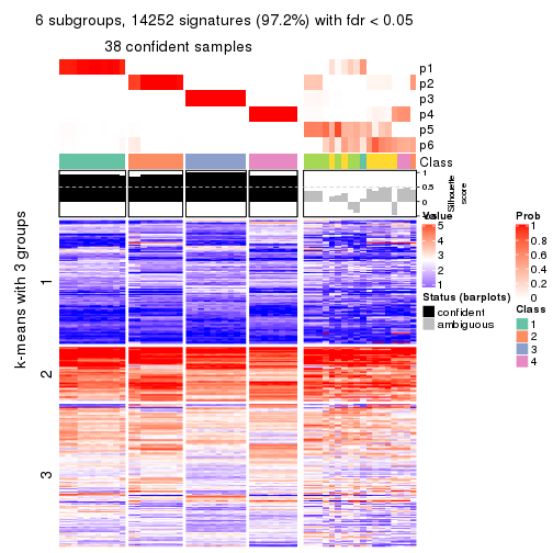
Compare the overlap of signatures from different k:
compare_signatures(res)
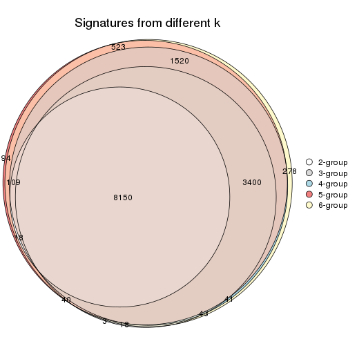
get_signature() returns a data frame invisibly. TO get the list of signatures, the function
call should be assigned to a variable explicitly. In following code, if plot argument is set
to FALSE, no heatmap is plotted while only the differential analysis is performed.
# code only for demonstration
tb = get_signature(res, k = ..., plot = FALSE)
An example of the output of tb is:
#> which_row fdr mean_1 mean_2 scaled_mean_1 scaled_mean_2 km
#> 1 38 0.042760348 8.373488 9.131774 -0.5533452 0.5164555 1
#> 2 40 0.018707592 7.106213 8.469186 -0.6173731 0.5762149 1
#> 3 55 0.019134737 10.221463 11.207825 -0.6159697 0.5749050 1
#> 4 59 0.006059896 5.921854 7.869574 -0.6899429 0.6439467 1
#> 5 60 0.018055526 8.928898 10.211722 -0.6204761 0.5791110 1
#> 6 98 0.009384629 15.714769 14.887706 0.6635654 -0.6193277 2
...
The columns in tb are:
which_row: row indices corresponding to the input matrix.fdr: FDR for the differential test. mean_x: The mean value in group x.scaled_mean_x: The mean value in group x after rows are scaled.km: Row groups if k-means clustering is applied to rows.UMAP plot which shows how samples are separated.
dimension_reduction(res, k = 2, method = "UMAP")
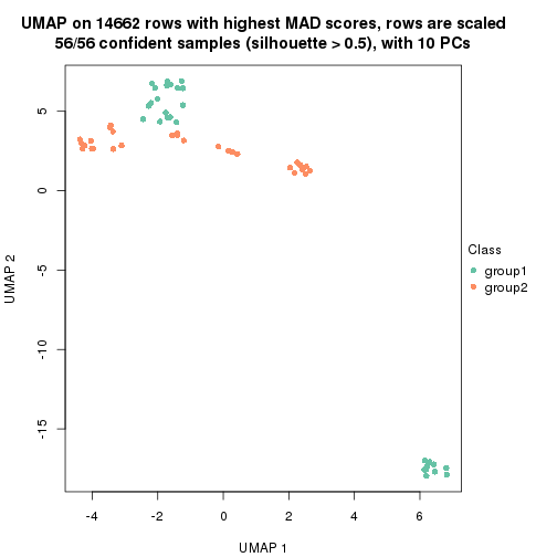
dimension_reduction(res, k = 3, method = "UMAP")
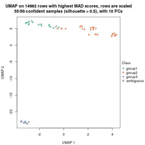
dimension_reduction(res, k = 4, method = "UMAP")

dimension_reduction(res, k = 5, method = "UMAP")
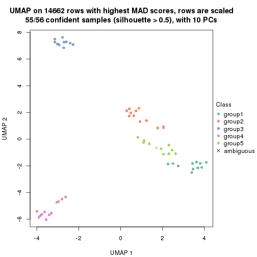
dimension_reduction(res, k = 6, method = "UMAP")
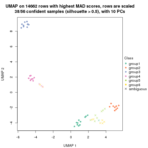
Following heatmap shows how subgroups are split when increasing k:
collect_classes(res)
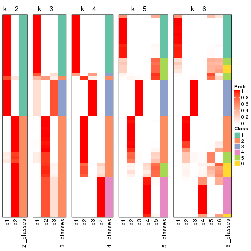
If matrix rows can be associated to genes, consider to use functional_enrichment(res,
...) to perform function enrichment for the signature genes. See this vignette for more detailed explanations.
The object with results only for a single top-value method and a single partition method can be extracted as:
res = res_list["ATC", "hclust"]
# you can also extract it by
# res = res_list["ATC:hclust"]
A summary of res and all the functions that can be applied to it:
res
#> A 'ConsensusPartition' object with k = 2, 3, 4, 5, 6.
#> On a matrix with 14662 rows and 56 columns.
#> Top rows (1000, 2000, 3000, 4000, 5000) are extracted by 'ATC' method.
#> Subgroups are detected by 'hclust' method.
#> Performed in total 1250 partitions by row resampling.
#> Best k for subgroups seems to be 4.
#>
#> Following methods can be applied to this 'ConsensusPartition' object:
#> [1] "cola_report" "collect_classes" "collect_plots"
#> [4] "collect_stats" "colnames" "compare_signatures"
#> [7] "consensus_heatmap" "dimension_reduction" "functional_enrichment"
#> [10] "get_anno_col" "get_anno" "get_classes"
#> [13] "get_consensus" "get_matrix" "get_membership"
#> [16] "get_param" "get_signatures" "get_stats"
#> [19] "is_best_k" "is_stable_k" "membership_heatmap"
#> [22] "ncol" "nrow" "plot_ecdf"
#> [25] "rownames" "select_partition_number" "show"
#> [28] "suggest_best_k" "test_to_known_factors"
collect_plots() function collects all the plots made from res for all k (number of partitions)
into one single page to provide an easy and fast comparison between different k.
collect_plots(res)
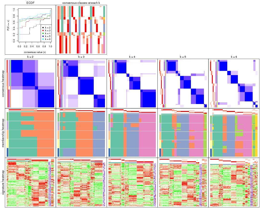
The plots are:
k and the heatmap of
predicted classes for each k.k.k.k.All the plots in panels can be made by individual functions and they are plotted later in this section.
select_partition_number() produces several plots showing different
statistics for choosing “optimized” k. There are following statistics:
k;k, the area increased is defined as \(A_k - A_{k-1}\).The detailed explanations of these statistics can be found in the cola vignette.
Generally speaking, lower PAC score, higher mean silhouette score or higher
concordance corresponds to better partition. Rand index and Jaccard index
measure how similar the current partition is compared to partition with k-1.
If they are too similar, we won't accept k is better than k-1.
select_partition_number(res)
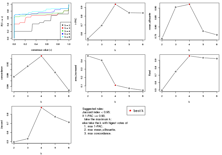
The numeric values for all these statistics can be obtained by get_stats().
get_stats(res)
#> k 1-PAC mean_silhouette concordance area_increased Rand Jaccard
#> 2 2 0.544 0.738 0.875 0.4583 0.497 0.497
#> 3 3 0.694 0.905 0.912 0.4057 0.748 0.532
#> 4 4 0.935 0.921 0.950 0.1079 0.958 0.873
#> 5 5 0.839 0.778 0.890 0.0704 0.934 0.773
#> 6 6 0.837 0.758 0.826 0.0471 0.923 0.713
suggest_best_k() suggests the best \(k\) based on these statistics. The rules are as follows:
suggest_best_k(res)
#> [1] 4
Following shows the table of the partitions (You need to click the show/hide
code output link to see it). The membership matrix (columns with name p*)
is inferred by
clue::cl_consensus()
function with the SE method. Basically the value in the membership matrix
represents the probability to belong to a certain group. The finall class
label for an item is determined with the group with highest probability it
belongs to.
In get_classes() function, the entropy is calculated from the membership
matrix and the silhouette score is calculated from the consensus matrix.
cbind(get_classes(res, k = 2), get_membership(res, k = 2))
#> class entropy silhouette p1 p2
#> SRR073723 1 0.900 0.724 0.684 0.316
#> SRR073724 1 0.000 0.775 1.000 0.000
#> SRR073725 1 0.000 0.775 1.000 0.000
#> SRR073726 2 0.992 -0.129 0.448 0.552
#> SRR073727 1 0.000 0.775 1.000 0.000
#> SRR073728 2 0.996 -0.186 0.464 0.536
#> SRR073729 2 0.996 -0.186 0.464 0.536
#> SRR073730 2 0.996 -0.186 0.464 0.536
#> SRR073731 2 0.000 0.896 0.000 1.000
#> SRR073732 2 0.000 0.896 0.000 1.000
#> SRR073733 2 0.000 0.896 0.000 1.000
#> SRR073734 2 0.000 0.896 0.000 1.000
#> SRR073735 2 0.000 0.896 0.000 1.000
#> SRR073736 2 0.000 0.896 0.000 1.000
#> SRR073737 2 0.000 0.896 0.000 1.000
#> SRR073738 1 0.000 0.775 1.000 0.000
#> SRR073739 1 0.909 0.723 0.676 0.324
#> SRR073740 1 0.909 0.723 0.676 0.324
#> SRR073741 1 0.909 0.723 0.676 0.324
#> SRR073742 1 0.909 0.723 0.676 0.324
#> SRR073743 1 0.909 0.723 0.676 0.324
#> SRR073744 1 0.909 0.723 0.676 0.324
#> SRR073745 1 0.909 0.723 0.676 0.324
#> SRR073746 1 0.909 0.723 0.676 0.324
#> SRR073747 1 0.909 0.723 0.676 0.324
#> SRR073748 1 0.909 0.723 0.676 0.324
#> SRR073749 1 0.909 0.723 0.676 0.324
#> SRR073750 1 0.000 0.775 1.000 0.000
#> SRR073751 1 0.909 0.723 0.676 0.324
#> SRR073752 2 0.000 0.896 0.000 1.000
#> SRR073753 2 0.000 0.896 0.000 1.000
#> SRR073754 1 0.909 0.723 0.676 0.324
#> SRR073755 2 0.000 0.896 0.000 1.000
#> SRR073756 2 0.000 0.896 0.000 1.000
#> SRR073758 2 0.000 0.896 0.000 1.000
#> SRR073759 2 0.000 0.896 0.000 1.000
#> SRR073760 2 0.000 0.896 0.000 1.000
#> SRR073761 2 0.000 0.896 0.000 1.000
#> SRR073763 2 0.000 0.896 0.000 1.000
#> SRR073764 2 0.000 0.896 0.000 1.000
#> SRR073765 2 0.000 0.896 0.000 1.000
#> SRR073766 2 0.000 0.896 0.000 1.000
#> SRR073767 2 0.000 0.896 0.000 1.000
#> SRR073768 2 0.000 0.896 0.000 1.000
#> SRR073769 1 0.000 0.775 1.000 0.000
#> SRR073770 1 0.000 0.775 1.000 0.000
#> SRR073771 1 0.000 0.775 1.000 0.000
#> SRR073772 1 0.000 0.775 1.000 0.000
#> SRR073773 1 0.000 0.775 1.000 0.000
#> SRR073774 1 0.000 0.775 1.000 0.000
#> SRR073775 1 0.000 0.775 1.000 0.000
#> SRR073776 1 0.000 0.775 1.000 0.000
#> SRR073777 1 0.000 0.775 1.000 0.000
#> SRR073778 1 0.000 0.775 1.000 0.000
#> SRR073779 1 0.909 0.723 0.676 0.324
#> SRR073780 1 0.909 0.723 0.676 0.324
cbind(get_classes(res, k = 3), get_membership(res, k = 3))
#> class entropy silhouette p1 p2 p3
#> SRR073723 1 0.470 0.868 0.788 0.000 0.212
#> SRR073724 3 0.312 0.894 0.108 0.000 0.892
#> SRR073725 3 0.312 0.894 0.108 0.000 0.892
#> SRR073726 1 0.493 0.558 0.768 0.232 0.000
#> SRR073727 3 0.312 0.894 0.108 0.000 0.892
#> SRR073728 1 0.877 0.696 0.588 0.212 0.200
#> SRR073729 1 0.877 0.696 0.588 0.212 0.200
#> SRR073730 1 0.877 0.696 0.588 0.212 0.200
#> SRR073731 2 0.000 0.984 0.000 1.000 0.000
#> SRR073732 2 0.000 0.984 0.000 1.000 0.000
#> SRR073733 2 0.000 0.984 0.000 1.000 0.000
#> SRR073734 2 0.000 0.984 0.000 1.000 0.000
#> SRR073735 2 0.000 0.984 0.000 1.000 0.000
#> SRR073736 2 0.000 0.984 0.000 1.000 0.000
#> SRR073737 2 0.000 0.984 0.000 1.000 0.000
#> SRR073738 3 0.312 0.894 0.108 0.000 0.892
#> SRR073739 1 0.455 0.879 0.800 0.000 0.200
#> SRR073740 1 0.455 0.879 0.800 0.000 0.200
#> SRR073741 1 0.455 0.879 0.800 0.000 0.200
#> SRR073742 1 0.455 0.879 0.800 0.000 0.200
#> SRR073743 1 0.455 0.879 0.800 0.000 0.200
#> SRR073744 1 0.455 0.879 0.800 0.000 0.200
#> SRR073745 1 0.455 0.879 0.800 0.000 0.200
#> SRR073746 1 0.455 0.879 0.800 0.000 0.200
#> SRR073747 1 0.455 0.879 0.800 0.000 0.200
#> SRR073748 1 0.455 0.879 0.800 0.000 0.200
#> SRR073749 1 0.455 0.879 0.800 0.000 0.200
#> SRR073750 3 0.312 0.894 0.108 0.000 0.892
#> SRR073751 1 0.455 0.879 0.800 0.000 0.200
#> SRR073752 2 0.288 0.894 0.096 0.904 0.000
#> SRR073753 2 0.288 0.894 0.096 0.904 0.000
#> SRR073754 1 0.000 0.751 1.000 0.000 0.000
#> SRR073755 2 0.000 0.984 0.000 1.000 0.000
#> SRR073756 2 0.000 0.984 0.000 1.000 0.000
#> SRR073758 2 0.000 0.984 0.000 1.000 0.000
#> SRR073759 2 0.288 0.894 0.096 0.904 0.000
#> SRR073760 2 0.000 0.984 0.000 1.000 0.000
#> SRR073761 2 0.000 0.984 0.000 1.000 0.000
#> SRR073763 2 0.000 0.984 0.000 1.000 0.000
#> SRR073764 2 0.000 0.984 0.000 1.000 0.000
#> SRR073765 2 0.000 0.984 0.000 1.000 0.000
#> SRR073766 2 0.000 0.984 0.000 1.000 0.000
#> SRR073767 2 0.000 0.984 0.000 1.000 0.000
#> SRR073768 2 0.000 0.984 0.000 1.000 0.000
#> SRR073769 3 0.000 0.952 0.000 0.000 1.000
#> SRR073770 3 0.000 0.952 0.000 0.000 1.000
#> SRR073771 3 0.000 0.952 0.000 0.000 1.000
#> SRR073772 3 0.000 0.952 0.000 0.000 1.000
#> SRR073773 3 0.000 0.952 0.000 0.000 1.000
#> SRR073774 3 0.000 0.952 0.000 0.000 1.000
#> SRR073775 3 0.000 0.952 0.000 0.000 1.000
#> SRR073776 3 0.000 0.952 0.000 0.000 1.000
#> SRR073777 3 0.000 0.952 0.000 0.000 1.000
#> SRR073778 3 0.000 0.952 0.000 0.000 1.000
#> SRR073779 1 0.000 0.751 1.000 0.000 0.000
#> SRR073780 1 0.000 0.751 1.000 0.000 0.000
cbind(get_classes(res, k = 4), get_membership(res, k = 4))
#> class entropy silhouette p1 p2 p3 p4
#> SRR073723 1 0.0804 0.903 0.980 0.008 0.012 0.000
#> SRR073724 3 0.2469 0.917 0.000 0.108 0.892 0.000
#> SRR073725 3 0.2469 0.917 0.000 0.108 0.892 0.000
#> SRR073726 2 0.3907 0.664 0.000 0.768 0.000 0.232
#> SRR073727 3 0.2469 0.917 0.000 0.108 0.892 0.000
#> SRR073728 1 0.5889 0.575 0.688 0.100 0.000 0.212
#> SRR073729 1 0.5889 0.575 0.688 0.100 0.000 0.212
#> SRR073730 1 0.5889 0.575 0.688 0.100 0.000 0.212
#> SRR073731 4 0.0000 0.983 0.000 0.000 0.000 1.000
#> SRR073732 4 0.0000 0.983 0.000 0.000 0.000 1.000
#> SRR073733 4 0.0000 0.983 0.000 0.000 0.000 1.000
#> SRR073734 4 0.0000 0.983 0.000 0.000 0.000 1.000
#> SRR073735 4 0.0000 0.983 0.000 0.000 0.000 1.000
#> SRR073736 4 0.0000 0.983 0.000 0.000 0.000 1.000
#> SRR073737 4 0.0000 0.983 0.000 0.000 0.000 1.000
#> SRR073738 3 0.2469 0.917 0.000 0.108 0.892 0.000
#> SRR073739 1 0.0000 0.918 1.000 0.000 0.000 0.000
#> SRR073740 1 0.0000 0.918 1.000 0.000 0.000 0.000
#> SRR073741 1 0.0000 0.918 1.000 0.000 0.000 0.000
#> SRR073742 1 0.0000 0.918 1.000 0.000 0.000 0.000
#> SRR073743 1 0.0000 0.918 1.000 0.000 0.000 0.000
#> SRR073744 1 0.0000 0.918 1.000 0.000 0.000 0.000
#> SRR073745 1 0.0000 0.918 1.000 0.000 0.000 0.000
#> SRR073746 1 0.0000 0.918 1.000 0.000 0.000 0.000
#> SRR073747 1 0.0000 0.918 1.000 0.000 0.000 0.000
#> SRR073748 1 0.0000 0.918 1.000 0.000 0.000 0.000
#> SRR073749 1 0.0000 0.918 1.000 0.000 0.000 0.000
#> SRR073750 3 0.2469 0.917 0.000 0.108 0.892 0.000
#> SRR073751 1 0.0469 0.912 0.988 0.012 0.000 0.000
#> SRR073752 4 0.2281 0.891 0.000 0.096 0.000 0.904
#> SRR073753 4 0.2281 0.891 0.000 0.096 0.000 0.904
#> SRR073754 2 0.0000 0.897 0.000 1.000 0.000 0.000
#> SRR073755 4 0.0000 0.983 0.000 0.000 0.000 1.000
#> SRR073756 4 0.0000 0.983 0.000 0.000 0.000 1.000
#> SRR073758 4 0.0000 0.983 0.000 0.000 0.000 1.000
#> SRR073759 4 0.2281 0.891 0.000 0.096 0.000 0.904
#> SRR073760 4 0.0000 0.983 0.000 0.000 0.000 1.000
#> SRR073761 4 0.0000 0.983 0.000 0.000 0.000 1.000
#> SRR073763 4 0.0000 0.983 0.000 0.000 0.000 1.000
#> SRR073764 4 0.0000 0.983 0.000 0.000 0.000 1.000
#> SRR073765 4 0.0000 0.983 0.000 0.000 0.000 1.000
#> SRR073766 4 0.0000 0.983 0.000 0.000 0.000 1.000
#> SRR073767 4 0.0000 0.983 0.000 0.000 0.000 1.000
#> SRR073768 4 0.0000 0.983 0.000 0.000 0.000 1.000
#> SRR073769 3 0.0000 0.960 0.000 0.000 1.000 0.000
#> SRR073770 3 0.0000 0.960 0.000 0.000 1.000 0.000
#> SRR073771 3 0.0000 0.960 0.000 0.000 1.000 0.000
#> SRR073772 3 0.0000 0.960 0.000 0.000 1.000 0.000
#> SRR073773 3 0.0000 0.960 0.000 0.000 1.000 0.000
#> SRR073774 3 0.0000 0.960 0.000 0.000 1.000 0.000
#> SRR073775 3 0.0000 0.960 0.000 0.000 1.000 0.000
#> SRR073776 3 0.0000 0.960 0.000 0.000 1.000 0.000
#> SRR073777 3 0.0000 0.960 0.000 0.000 1.000 0.000
#> SRR073778 3 0.0000 0.960 0.000 0.000 1.000 0.000
#> SRR073779 2 0.0000 0.897 0.000 1.000 0.000 0.000
#> SRR073780 2 0.0000 0.897 0.000 1.000 0.000 0.000
cbind(get_classes(res, k = 5), get_membership(res, k = 5))
#> class entropy silhouette p1 p2 p3 p4 p5
#> SRR073723 1 0.384 0.6435 0.736 0.256 0.004 0.000 0.004
#> SRR073724 3 0.338 0.8772 0.000 0.056 0.840 0.000 0.104
#> SRR073725 3 0.338 0.8772 0.000 0.056 0.840 0.000 0.104
#> SRR073726 5 0.433 0.5978 0.000 0.312 0.000 0.016 0.672
#> SRR073727 3 0.338 0.8772 0.000 0.056 0.840 0.000 0.104
#> SRR073728 2 0.442 0.0575 0.444 0.552 0.000 0.000 0.004
#> SRR073729 2 0.442 0.0575 0.444 0.552 0.000 0.000 0.004
#> SRR073730 2 0.442 0.0575 0.444 0.552 0.000 0.000 0.004
#> SRR073731 4 0.364 0.7357 0.000 0.272 0.000 0.728 0.000
#> SRR073732 4 0.364 0.7357 0.000 0.272 0.000 0.728 0.000
#> SRR073733 4 0.364 0.7357 0.000 0.272 0.000 0.728 0.000
#> SRR073734 4 0.364 0.7357 0.000 0.272 0.000 0.728 0.000
#> SRR073735 4 0.364 0.7357 0.000 0.272 0.000 0.728 0.000
#> SRR073736 4 0.364 0.7357 0.000 0.272 0.000 0.728 0.000
#> SRR073737 4 0.364 0.7357 0.000 0.272 0.000 0.728 0.000
#> SRR073738 3 0.338 0.8772 0.000 0.056 0.840 0.000 0.104
#> SRR073739 1 0.000 0.9483 1.000 0.000 0.000 0.000 0.000
#> SRR073740 1 0.000 0.9483 1.000 0.000 0.000 0.000 0.000
#> SRR073741 1 0.000 0.9483 1.000 0.000 0.000 0.000 0.000
#> SRR073742 1 0.000 0.9483 1.000 0.000 0.000 0.000 0.000
#> SRR073743 1 0.000 0.9483 1.000 0.000 0.000 0.000 0.000
#> SRR073744 1 0.000 0.9483 1.000 0.000 0.000 0.000 0.000
#> SRR073745 1 0.000 0.9483 1.000 0.000 0.000 0.000 0.000
#> SRR073746 1 0.000 0.9483 1.000 0.000 0.000 0.000 0.000
#> SRR073747 1 0.000 0.9483 1.000 0.000 0.000 0.000 0.000
#> SRR073748 1 0.000 0.9483 1.000 0.000 0.000 0.000 0.000
#> SRR073749 1 0.000 0.9483 1.000 0.000 0.000 0.000 0.000
#> SRR073750 3 0.338 0.8772 0.000 0.056 0.840 0.000 0.104
#> SRR073751 1 0.384 0.6494 0.744 0.244 0.000 0.000 0.012
#> SRR073752 2 0.422 -0.0503 0.000 0.584 0.000 0.416 0.000
#> SRR073753 2 0.422 -0.0503 0.000 0.584 0.000 0.416 0.000
#> SRR073754 5 0.000 0.8901 0.000 0.000 0.000 0.000 1.000
#> SRR073755 4 0.000 0.8526 0.000 0.000 0.000 1.000 0.000
#> SRR073756 4 0.000 0.8526 0.000 0.000 0.000 1.000 0.000
#> SRR073758 4 0.000 0.8526 0.000 0.000 0.000 1.000 0.000
#> SRR073759 2 0.380 0.1536 0.000 0.700 0.000 0.300 0.000
#> SRR073760 4 0.000 0.8526 0.000 0.000 0.000 1.000 0.000
#> SRR073761 4 0.000 0.8526 0.000 0.000 0.000 1.000 0.000
#> SRR073763 4 0.000 0.8526 0.000 0.000 0.000 1.000 0.000
#> SRR073764 4 0.000 0.8526 0.000 0.000 0.000 1.000 0.000
#> SRR073765 4 0.000 0.8526 0.000 0.000 0.000 1.000 0.000
#> SRR073766 4 0.000 0.8526 0.000 0.000 0.000 1.000 0.000
#> SRR073767 4 0.000 0.8526 0.000 0.000 0.000 1.000 0.000
#> SRR073768 4 0.000 0.8526 0.000 0.000 0.000 1.000 0.000
#> SRR073769 3 0.000 0.9428 0.000 0.000 1.000 0.000 0.000
#> SRR073770 3 0.000 0.9428 0.000 0.000 1.000 0.000 0.000
#> SRR073771 3 0.000 0.9428 0.000 0.000 1.000 0.000 0.000
#> SRR073772 3 0.000 0.9428 0.000 0.000 1.000 0.000 0.000
#> SRR073773 3 0.000 0.9428 0.000 0.000 1.000 0.000 0.000
#> SRR073774 3 0.000 0.9428 0.000 0.000 1.000 0.000 0.000
#> SRR073775 3 0.000 0.9428 0.000 0.000 1.000 0.000 0.000
#> SRR073776 3 0.000 0.9428 0.000 0.000 1.000 0.000 0.000
#> SRR073777 3 0.000 0.9428 0.000 0.000 1.000 0.000 0.000
#> SRR073778 3 0.000 0.9428 0.000 0.000 1.000 0.000 0.000
#> SRR073779 5 0.000 0.8901 0.000 0.000 0.000 0.000 1.000
#> SRR073780 5 0.000 0.8901 0.000 0.000 0.000 0.000 1.000
cbind(get_classes(res, k = 6), get_membership(res, k = 6))
#> class entropy silhouette p1 p2 p3 p4 p5 p6
#> SRR073723 1 0.577 -0.04416 0.528 0.048 0.000 0.000 0.356 0.068
#> SRR073724 2 0.317 1.00000 0.000 0.744 0.256 0.000 0.000 0.000
#> SRR073725 2 0.317 1.00000 0.000 0.744 0.256 0.000 0.000 0.000
#> SRR073726 5 0.580 -0.55251 0.000 0.212 0.000 0.004 0.524 0.260
#> SRR073727 2 0.317 1.00000 0.000 0.744 0.256 0.000 0.000 0.000
#> SRR073728 5 0.352 0.67828 0.324 0.000 0.000 0.000 0.676 0.000
#> SRR073729 5 0.352 0.67828 0.324 0.000 0.000 0.000 0.676 0.000
#> SRR073730 5 0.352 0.67828 0.324 0.000 0.000 0.000 0.676 0.000
#> SRR073731 4 0.000 0.66562 0.000 0.000 0.000 1.000 0.000 0.000
#> SRR073732 4 0.000 0.66562 0.000 0.000 0.000 1.000 0.000 0.000
#> SRR073733 4 0.000 0.66562 0.000 0.000 0.000 1.000 0.000 0.000
#> SRR073734 4 0.000 0.66562 0.000 0.000 0.000 1.000 0.000 0.000
#> SRR073735 4 0.000 0.66562 0.000 0.000 0.000 1.000 0.000 0.000
#> SRR073736 4 0.000 0.66562 0.000 0.000 0.000 1.000 0.000 0.000
#> SRR073737 4 0.000 0.66562 0.000 0.000 0.000 1.000 0.000 0.000
#> SRR073738 2 0.317 1.00000 0.000 0.744 0.256 0.000 0.000 0.000
#> SRR073739 1 0.000 0.89639 1.000 0.000 0.000 0.000 0.000 0.000
#> SRR073740 1 0.000 0.89639 1.000 0.000 0.000 0.000 0.000 0.000
#> SRR073741 1 0.000 0.89639 1.000 0.000 0.000 0.000 0.000 0.000
#> SRR073742 1 0.000 0.89639 1.000 0.000 0.000 0.000 0.000 0.000
#> SRR073743 1 0.000 0.89639 1.000 0.000 0.000 0.000 0.000 0.000
#> SRR073744 1 0.000 0.89639 1.000 0.000 0.000 0.000 0.000 0.000
#> SRR073745 1 0.000 0.89639 1.000 0.000 0.000 0.000 0.000 0.000
#> SRR073746 1 0.000 0.89639 1.000 0.000 0.000 0.000 0.000 0.000
#> SRR073747 1 0.000 0.89639 1.000 0.000 0.000 0.000 0.000 0.000
#> SRR073748 1 0.000 0.89639 1.000 0.000 0.000 0.000 0.000 0.000
#> SRR073749 1 0.000 0.89639 1.000 0.000 0.000 0.000 0.000 0.000
#> SRR073750 2 0.317 1.00000 0.000 0.744 0.256 0.000 0.000 0.000
#> SRR073751 1 0.559 -0.05908 0.528 0.028 0.000 0.000 0.368 0.076
#> SRR073752 4 0.364 0.24833 0.000 0.000 0.000 0.676 0.320 0.004
#> SRR073753 4 0.364 0.24833 0.000 0.000 0.000 0.676 0.320 0.004
#> SRR073754 6 0.572 1.00000 0.000 0.284 0.000 0.000 0.204 0.512
#> SRR073755 4 0.379 0.73047 0.000 0.000 0.000 0.584 0.000 0.416
#> SRR073756 4 0.379 0.73047 0.000 0.000 0.000 0.584 0.000 0.416
#> SRR073758 4 0.379 0.73047 0.000 0.000 0.000 0.584 0.000 0.416
#> SRR073759 4 0.436 -0.00193 0.000 0.016 0.000 0.548 0.432 0.004
#> SRR073760 4 0.379 0.73047 0.000 0.000 0.000 0.584 0.000 0.416
#> SRR073761 4 0.379 0.73047 0.000 0.000 0.000 0.584 0.000 0.416
#> SRR073763 4 0.379 0.73047 0.000 0.000 0.000 0.584 0.000 0.416
#> SRR073764 4 0.379 0.73047 0.000 0.000 0.000 0.584 0.000 0.416
#> SRR073765 4 0.379 0.73047 0.000 0.000 0.000 0.584 0.000 0.416
#> SRR073766 4 0.379 0.73047 0.000 0.000 0.000 0.584 0.000 0.416
#> SRR073767 4 0.379 0.73047 0.000 0.000 0.000 0.584 0.000 0.416
#> SRR073768 4 0.379 0.73047 0.000 0.000 0.000 0.584 0.000 0.416
#> SRR073769 3 0.000 1.00000 0.000 0.000 1.000 0.000 0.000 0.000
#> SRR073770 3 0.000 1.00000 0.000 0.000 1.000 0.000 0.000 0.000
#> SRR073771 3 0.000 1.00000 0.000 0.000 1.000 0.000 0.000 0.000
#> SRR073772 3 0.000 1.00000 0.000 0.000 1.000 0.000 0.000 0.000
#> SRR073773 3 0.000 1.00000 0.000 0.000 1.000 0.000 0.000 0.000
#> SRR073774 3 0.000 1.00000 0.000 0.000 1.000 0.000 0.000 0.000
#> SRR073775 3 0.000 1.00000 0.000 0.000 1.000 0.000 0.000 0.000
#> SRR073776 3 0.000 1.00000 0.000 0.000 1.000 0.000 0.000 0.000
#> SRR073777 3 0.000 1.00000 0.000 0.000 1.000 0.000 0.000 0.000
#> SRR073778 3 0.000 1.00000 0.000 0.000 1.000 0.000 0.000 0.000
#> SRR073779 6 0.572 1.00000 0.000 0.284 0.000 0.000 0.204 0.512
#> SRR073780 6 0.572 1.00000 0.000 0.284 0.000 0.000 0.204 0.512
Heatmaps for the consensus matrix. It visualizes the probability of two samples to be in a same group.
consensus_heatmap(res, k = 2)
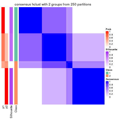
consensus_heatmap(res, k = 3)
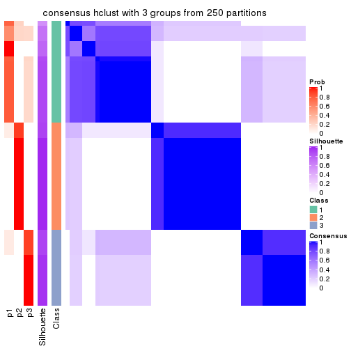
consensus_heatmap(res, k = 4)
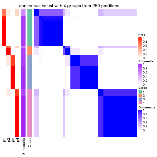
consensus_heatmap(res, k = 5)
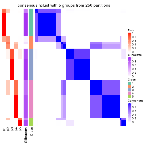
consensus_heatmap(res, k = 6)
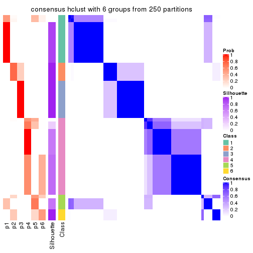
Heatmaps for the membership of samples in all partitions to see how consistent they are:
membership_heatmap(res, k = 2)
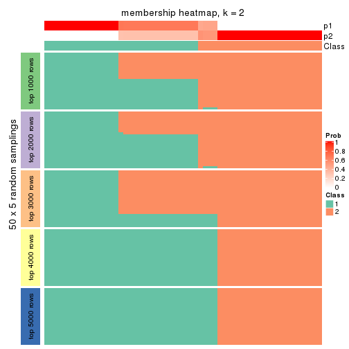
membership_heatmap(res, k = 3)
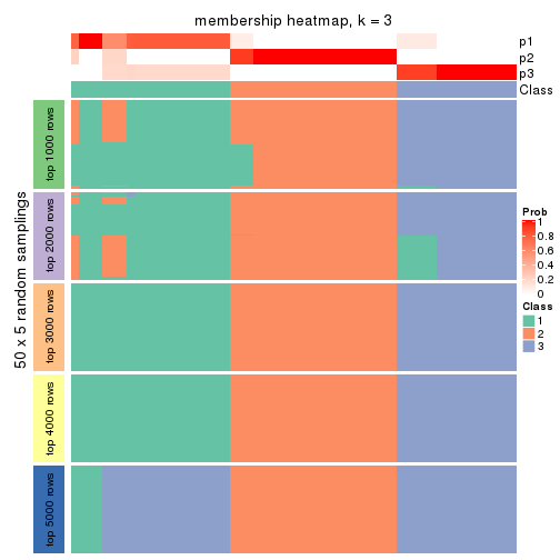
membership_heatmap(res, k = 4)
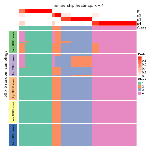
membership_heatmap(res, k = 5)
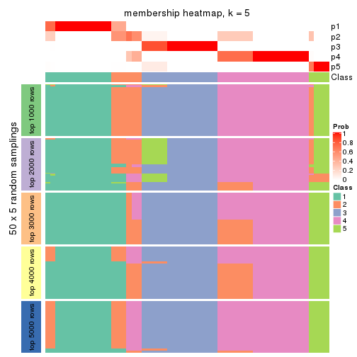
membership_heatmap(res, k = 6)
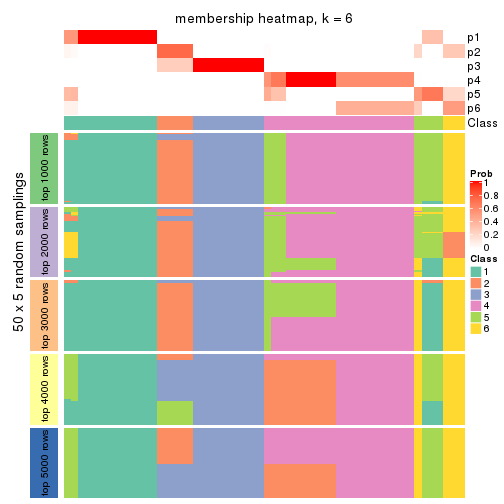
As soon as we have had the classes for columns, we can look for signatures which are significantly different between classes which can be candidate marks for certain classes. Following are the heatmaps for signatures.
Signature heatmaps where rows are scaled:
get_signatures(res, k = 2)
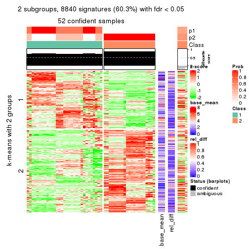
get_signatures(res, k = 3)
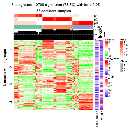
get_signatures(res, k = 4)
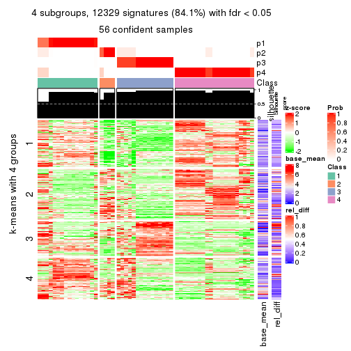
get_signatures(res, k = 5)
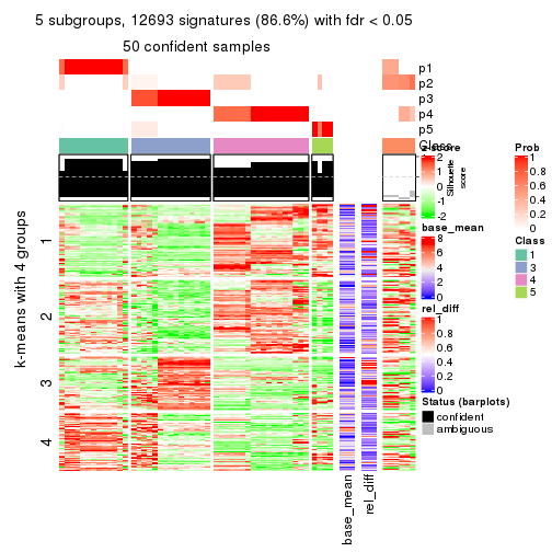
get_signatures(res, k = 6)
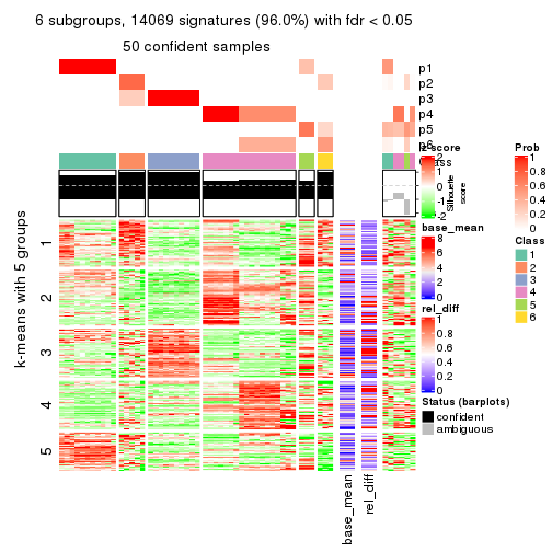
Signature heatmaps where rows are not scaled:
get_signatures(res, k = 2, scale_rows = FALSE)
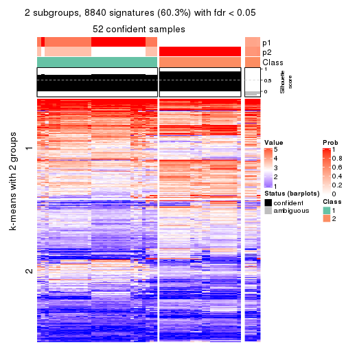
get_signatures(res, k = 3, scale_rows = FALSE)
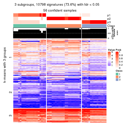
get_signatures(res, k = 4, scale_rows = FALSE)
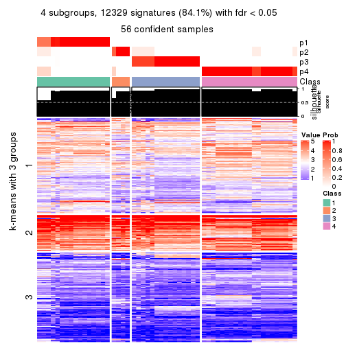
get_signatures(res, k = 5, scale_rows = FALSE)
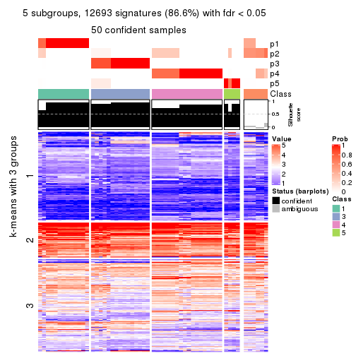
get_signatures(res, k = 6, scale_rows = FALSE)
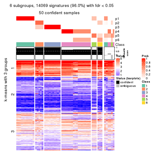
Compare the overlap of signatures from different k:
compare_signatures(res)
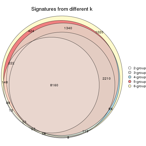
get_signature() returns a data frame invisibly. TO get the list of signatures, the function
call should be assigned to a variable explicitly. In following code, if plot argument is set
to FALSE, no heatmap is plotted while only the differential analysis is performed.
# code only for demonstration
tb = get_signature(res, k = ..., plot = FALSE)
An example of the output of tb is:
#> which_row fdr mean_1 mean_2 scaled_mean_1 scaled_mean_2 km
#> 1 38 0.042760348 8.373488 9.131774 -0.5533452 0.5164555 1
#> 2 40 0.018707592 7.106213 8.469186 -0.6173731 0.5762149 1
#> 3 55 0.019134737 10.221463 11.207825 -0.6159697 0.5749050 1
#> 4 59 0.006059896 5.921854 7.869574 -0.6899429 0.6439467 1
#> 5 60 0.018055526 8.928898 10.211722 -0.6204761 0.5791110 1
#> 6 98 0.009384629 15.714769 14.887706 0.6635654 -0.6193277 2
...
The columns in tb are:
which_row: row indices corresponding to the input matrix.fdr: FDR for the differential test. mean_x: The mean value in group x.scaled_mean_x: The mean value in group x after rows are scaled.km: Row groups if k-means clustering is applied to rows.UMAP plot which shows how samples are separated.
dimension_reduction(res, k = 2, method = "UMAP")
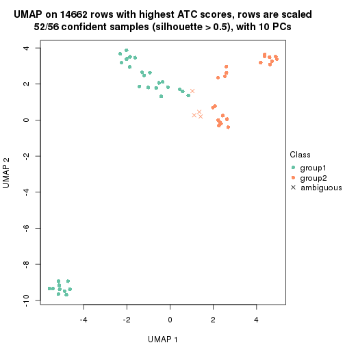
dimension_reduction(res, k = 3, method = "UMAP")
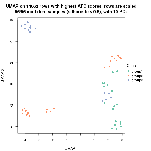
dimension_reduction(res, k = 4, method = "UMAP")
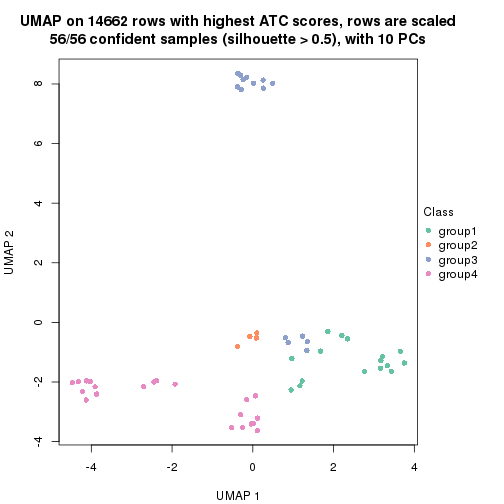
dimension_reduction(res, k = 5, method = "UMAP")
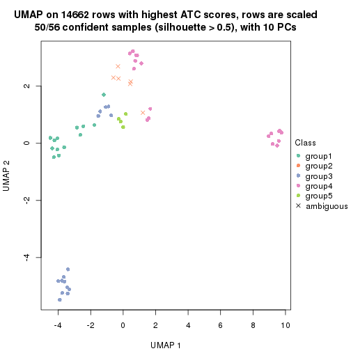
dimension_reduction(res, k = 6, method = "UMAP")
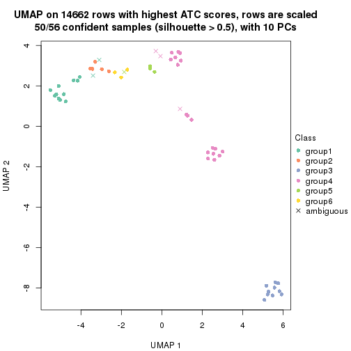
Following heatmap shows how subgroups are split when increasing k:
collect_classes(res)
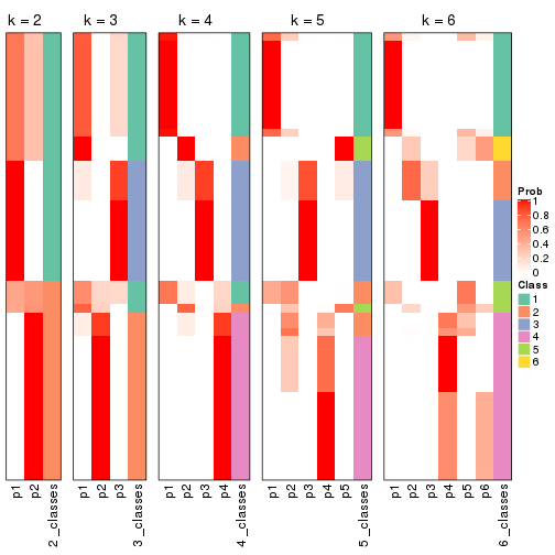
If matrix rows can be associated to genes, consider to use functional_enrichment(res,
...) to perform function enrichment for the signature genes. See this vignette for more detailed explanations.
The object with results only for a single top-value method and a single partition method can be extracted as:
res = res_list["ATC", "kmeans"]
# you can also extract it by
# res = res_list["ATC:kmeans"]
A summary of res and all the functions that can be applied to it:
res
#> A 'ConsensusPartition' object with k = 2, 3, 4, 5, 6.
#> On a matrix with 14662 rows and 56 columns.
#> Top rows (1000, 2000, 3000, 4000, 5000) are extracted by 'ATC' method.
#> Subgroups are detected by 'kmeans' method.
#> Performed in total 1250 partitions by row resampling.
#> Best k for subgroups seems to be 2.
#>
#> Following methods can be applied to this 'ConsensusPartition' object:
#> [1] "cola_report" "collect_classes" "collect_plots"
#> [4] "collect_stats" "colnames" "compare_signatures"
#> [7] "consensus_heatmap" "dimension_reduction" "functional_enrichment"
#> [10] "get_anno_col" "get_anno" "get_classes"
#> [13] "get_consensus" "get_matrix" "get_membership"
#> [16] "get_param" "get_signatures" "get_stats"
#> [19] "is_best_k" "is_stable_k" "membership_heatmap"
#> [22] "ncol" "nrow" "plot_ecdf"
#> [25] "rownames" "select_partition_number" "show"
#> [28] "suggest_best_k" "test_to_known_factors"
collect_plots() function collects all the plots made from res for all k (number of partitions)
into one single page to provide an easy and fast comparison between different k.
collect_plots(res)
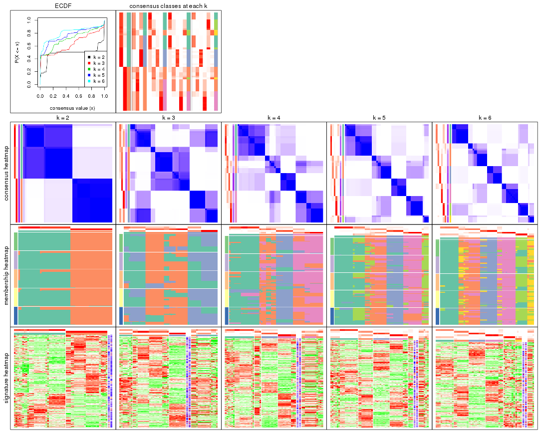
The plots are:
k and the heatmap of
predicted classes for each k.k.k.k.All the plots in panels can be made by individual functions and they are plotted later in this section.
select_partition_number() produces several plots showing different
statistics for choosing “optimized” k. There are following statistics:
k;k, the area increased is defined as \(A_k - A_{k-1}\).The detailed explanations of these statistics can be found in the cola vignette.
Generally speaking, lower PAC score, higher mean silhouette score or higher
concordance corresponds to better partition. Rand index and Jaccard index
measure how similar the current partition is compared to partition with k-1.
If they are too similar, we won't accept k is better than k-1.
select_partition_number(res)
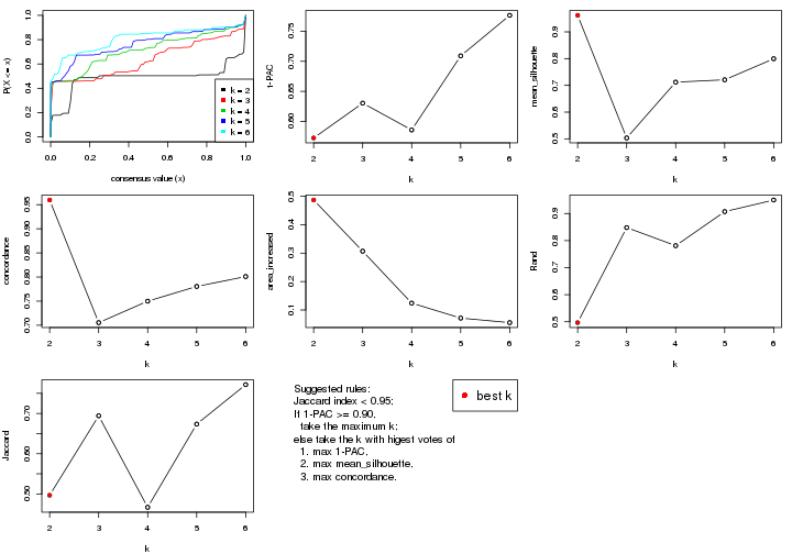
The numeric values for all these statistics can be obtained by get_stats().
get_stats(res)
#> k 1-PAC mean_silhouette concordance area_increased Rand Jaccard
#> 2 2 0.572 0.962 0.960 0.4868 0.497 0.497
#> 3 3 0.630 0.503 0.705 0.3068 0.848 0.694
#> 4 4 0.586 0.712 0.750 0.1241 0.781 0.467
#> 5 5 0.709 0.721 0.780 0.0714 0.907 0.674
#> 6 6 0.776 0.800 0.801 0.0555 0.950 0.772
suggest_best_k() suggests the best \(k\) based on these statistics. The rules are as follows:
suggest_best_k(res)
#> [1] 2
Following shows the table of the partitions (You need to click the show/hide
code output link to see it). The membership matrix (columns with name p*)
is inferred by
clue::cl_consensus()
function with the SE method. Basically the value in the membership matrix
represents the probability to belong to a certain group. The finall class
label for an item is determined with the group with highest probability it
belongs to.
In get_classes() function, the entropy is calculated from the membership
matrix and the silhouette score is calculated from the consensus matrix.
cbind(get_classes(res, k = 2), get_membership(res, k = 2))
#> class entropy silhouette p1 p2
#> SRR073723 1 0.4815 0.950 0.896 0.104
#> SRR073724 1 0.4815 0.950 0.896 0.104
#> SRR073725 1 0.0376 0.925 0.996 0.004
#> SRR073726 2 0.0000 0.997 0.000 1.000
#> SRR073727 1 0.4815 0.950 0.896 0.104
#> SRR073728 2 0.0672 0.991 0.008 0.992
#> SRR073729 2 0.0672 0.991 0.008 0.992
#> SRR073730 2 0.0672 0.991 0.008 0.992
#> SRR073731 2 0.0000 0.997 0.000 1.000
#> SRR073732 2 0.0000 0.997 0.000 1.000
#> SRR073733 2 0.0000 0.997 0.000 1.000
#> SRR073734 2 0.0000 0.997 0.000 1.000
#> SRR073735 2 0.0000 0.997 0.000 1.000
#> SRR073736 2 0.0000 0.997 0.000 1.000
#> SRR073737 2 0.0000 0.997 0.000 1.000
#> SRR073738 1 0.4815 0.950 0.896 0.104
#> SRR073739 1 0.4815 0.950 0.896 0.104
#> SRR073740 1 0.4815 0.950 0.896 0.104
#> SRR073741 1 0.4815 0.950 0.896 0.104
#> SRR073742 1 0.4815 0.950 0.896 0.104
#> SRR073743 1 0.4815 0.950 0.896 0.104
#> SRR073744 1 0.4815 0.950 0.896 0.104
#> SRR073745 1 0.4815 0.950 0.896 0.104
#> SRR073746 1 0.4815 0.950 0.896 0.104
#> SRR073747 1 0.4815 0.950 0.896 0.104
#> SRR073748 1 0.4815 0.950 0.896 0.104
#> SRR073749 1 0.4815 0.950 0.896 0.104
#> SRR073750 1 0.3114 0.939 0.944 0.056
#> SRR073751 1 0.4815 0.950 0.896 0.104
#> SRR073752 2 0.0000 0.997 0.000 1.000
#> SRR073753 2 0.0000 0.997 0.000 1.000
#> SRR073754 1 0.4815 0.950 0.896 0.104
#> SRR073755 2 0.0000 0.997 0.000 1.000
#> SRR073756 2 0.0000 0.997 0.000 1.000
#> SRR073758 2 0.0000 0.997 0.000 1.000
#> SRR073759 2 0.0000 0.997 0.000 1.000
#> SRR073760 2 0.0376 0.996 0.004 0.996
#> SRR073761 2 0.0376 0.996 0.004 0.996
#> SRR073763 2 0.0376 0.996 0.004 0.996
#> SRR073764 2 0.0376 0.996 0.004 0.996
#> SRR073765 2 0.0376 0.996 0.004 0.996
#> SRR073766 2 0.0376 0.996 0.004 0.996
#> SRR073767 2 0.0376 0.996 0.004 0.996
#> SRR073768 2 0.0376 0.996 0.004 0.996
#> SRR073769 1 0.0000 0.924 1.000 0.000
#> SRR073770 1 0.0000 0.924 1.000 0.000
#> SRR073771 1 0.0000 0.924 1.000 0.000
#> SRR073772 1 0.0000 0.924 1.000 0.000
#> SRR073773 1 0.0000 0.924 1.000 0.000
#> SRR073774 1 0.0000 0.924 1.000 0.000
#> SRR073775 1 0.0000 0.924 1.000 0.000
#> SRR073776 1 0.0000 0.924 1.000 0.000
#> SRR073777 1 0.0000 0.924 1.000 0.000
#> SRR073778 1 0.0000 0.924 1.000 0.000
#> SRR073779 1 0.5842 0.918 0.860 0.140
#> SRR073780 1 0.8016 0.787 0.756 0.244
cbind(get_classes(res, k = 3), get_membership(res, k = 3))
#> class entropy silhouette p1 p2 p3
#> SRR073723 1 0.6267 0.559 0.548 0.000 0.452
#> SRR073724 1 0.6267 0.559 0.548 0.000 0.452
#> SRR073725 3 0.6309 -0.464 0.496 0.000 0.504
#> SRR073726 2 0.4504 0.711 0.196 0.804 0.000
#> SRR073727 1 0.6267 0.559 0.548 0.000 0.452
#> SRR073728 2 0.6192 0.364 0.420 0.580 0.000
#> SRR073729 2 0.6192 0.364 0.420 0.580 0.000
#> SRR073730 2 0.6192 0.364 0.420 0.580 0.000
#> SRR073731 2 0.0424 0.801 0.008 0.992 0.000
#> SRR073732 2 0.1753 0.805 0.048 0.952 0.000
#> SRR073733 2 0.0424 0.801 0.008 0.992 0.000
#> SRR073734 2 0.0424 0.801 0.008 0.992 0.000
#> SRR073735 2 0.0424 0.801 0.008 0.992 0.000
#> SRR073736 2 0.0424 0.801 0.008 0.992 0.000
#> SRR073737 2 0.0424 0.801 0.008 0.992 0.000
#> SRR073738 1 0.6267 0.559 0.548 0.000 0.452
#> SRR073739 3 0.6291 -0.328 0.468 0.000 0.532
#> SRR073740 3 0.6291 -0.328 0.468 0.000 0.532
#> SRR073741 3 0.6291 -0.328 0.468 0.000 0.532
#> SRR073742 3 0.6291 -0.328 0.468 0.000 0.532
#> SRR073743 3 0.6291 -0.328 0.468 0.000 0.532
#> SRR073744 3 0.6291 -0.328 0.468 0.000 0.532
#> SRR073745 3 0.6291 -0.328 0.468 0.000 0.532
#> SRR073746 1 0.6305 0.460 0.516 0.000 0.484
#> SRR073747 1 0.6274 0.554 0.544 0.000 0.456
#> SRR073748 1 0.6274 0.554 0.544 0.000 0.456
#> SRR073749 1 0.6274 0.554 0.544 0.000 0.456
#> SRR073750 1 0.6280 0.541 0.540 0.000 0.460
#> SRR073751 1 0.5591 0.466 0.696 0.000 0.304
#> SRR073752 2 0.3686 0.743 0.140 0.860 0.000
#> SRR073753 2 0.3686 0.743 0.140 0.860 0.000
#> SRR073754 1 0.5812 0.360 0.724 0.264 0.012
#> SRR073755 2 0.5327 0.799 0.272 0.728 0.000
#> SRR073756 2 0.5327 0.799 0.272 0.728 0.000
#> SRR073758 2 0.5327 0.799 0.272 0.728 0.000
#> SRR073759 2 0.4002 0.738 0.160 0.840 0.000
#> SRR073760 2 0.5254 0.802 0.264 0.736 0.000
#> SRR073761 2 0.5254 0.802 0.264 0.736 0.000
#> SRR073763 2 0.5254 0.802 0.264 0.736 0.000
#> SRR073764 2 0.5254 0.802 0.264 0.736 0.000
#> SRR073765 2 0.5254 0.802 0.264 0.736 0.000
#> SRR073766 2 0.5254 0.802 0.264 0.736 0.000
#> SRR073767 2 0.5254 0.802 0.264 0.736 0.000
#> SRR073768 2 0.5254 0.802 0.264 0.736 0.000
#> SRR073769 3 0.0000 0.605 0.000 0.000 1.000
#> SRR073770 3 0.0000 0.605 0.000 0.000 1.000
#> SRR073771 3 0.0000 0.605 0.000 0.000 1.000
#> SRR073772 3 0.0000 0.605 0.000 0.000 1.000
#> SRR073773 3 0.0000 0.605 0.000 0.000 1.000
#> SRR073774 3 0.0000 0.605 0.000 0.000 1.000
#> SRR073775 3 0.0000 0.605 0.000 0.000 1.000
#> SRR073776 3 0.0000 0.605 0.000 0.000 1.000
#> SRR073777 3 0.0000 0.605 0.000 0.000 1.000
#> SRR073778 3 0.0000 0.605 0.000 0.000 1.000
#> SRR073779 1 0.5812 0.360 0.724 0.264 0.012
#> SRR073780 1 0.5812 0.360 0.724 0.264 0.012
cbind(get_classes(res, k = 4), get_membership(res, k = 4))
#> class entropy silhouette p1 p2 p3 p4
#> SRR073723 1 0.350 0.813 0.832 0.160 0.008 0.000
#> SRR073724 1 0.335 0.815 0.836 0.160 0.004 0.000
#> SRR073725 1 0.321 0.819 0.848 0.148 0.004 0.000
#> SRR073726 2 0.468 0.515 0.000 0.768 0.040 0.192
#> SRR073727 1 0.335 0.815 0.836 0.160 0.004 0.000
#> SRR073728 2 0.711 0.599 0.192 0.624 0.020 0.164
#> SRR073729 2 0.711 0.599 0.192 0.624 0.020 0.164
#> SRR073730 2 0.711 0.599 0.192 0.624 0.020 0.164
#> SRR073731 4 0.687 0.408 0.004 0.356 0.100 0.540
#> SRR073732 4 0.681 0.431 0.004 0.336 0.100 0.560
#> SRR073733 4 0.687 0.408 0.004 0.356 0.100 0.540
#> SRR073734 4 0.687 0.408 0.004 0.356 0.100 0.540
#> SRR073735 4 0.687 0.408 0.004 0.356 0.100 0.540
#> SRR073736 4 0.687 0.408 0.004 0.356 0.100 0.540
#> SRR073737 4 0.687 0.408 0.004 0.356 0.100 0.540
#> SRR073738 1 0.335 0.815 0.836 0.160 0.004 0.000
#> SRR073739 1 0.208 0.839 0.916 0.000 0.084 0.000
#> SRR073740 1 0.208 0.839 0.916 0.000 0.084 0.000
#> SRR073741 1 0.208 0.839 0.916 0.000 0.084 0.000
#> SRR073742 1 0.208 0.839 0.916 0.000 0.084 0.000
#> SRR073743 1 0.208 0.839 0.916 0.000 0.084 0.000
#> SRR073744 1 0.208 0.839 0.916 0.000 0.084 0.000
#> SRR073745 1 0.208 0.839 0.916 0.000 0.084 0.000
#> SRR073746 1 0.112 0.853 0.964 0.000 0.036 0.000
#> SRR073747 1 0.000 0.856 1.000 0.000 0.000 0.000
#> SRR073748 1 0.000 0.856 1.000 0.000 0.000 0.000
#> SRR073749 1 0.000 0.856 1.000 0.000 0.000 0.000
#> SRR073750 1 0.302 0.821 0.852 0.148 0.000 0.000
#> SRR073751 1 0.511 0.562 0.656 0.328 0.016 0.000
#> SRR073752 2 0.612 0.237 0.004 0.588 0.048 0.360
#> SRR073753 2 0.612 0.237 0.004 0.588 0.048 0.360
#> SRR073754 2 0.494 0.493 0.220 0.740 0.040 0.000
#> SRR073755 4 0.287 0.699 0.000 0.032 0.072 0.896
#> SRR073756 4 0.287 0.699 0.000 0.032 0.072 0.896
#> SRR073758 4 0.287 0.699 0.000 0.032 0.072 0.896
#> SRR073759 2 0.639 0.276 0.004 0.584 0.068 0.344
#> SRR073760 4 0.000 0.721 0.000 0.000 0.000 1.000
#> SRR073761 4 0.000 0.721 0.000 0.000 0.000 1.000
#> SRR073763 4 0.000 0.721 0.000 0.000 0.000 1.000
#> SRR073764 4 0.000 0.721 0.000 0.000 0.000 1.000
#> SRR073765 4 0.000 0.721 0.000 0.000 0.000 1.000
#> SRR073766 4 0.000 0.721 0.000 0.000 0.000 1.000
#> SRR073767 4 0.000 0.721 0.000 0.000 0.000 1.000
#> SRR073768 4 0.000 0.721 0.000 0.000 0.000 1.000
#> SRR073769 3 0.369 0.986 0.208 0.000 0.792 0.000
#> SRR073770 3 0.474 0.979 0.208 0.036 0.756 0.000
#> SRR073771 3 0.369 0.986 0.208 0.000 0.792 0.000
#> SRR073772 3 0.474 0.979 0.208 0.036 0.756 0.000
#> SRR073773 3 0.474 0.979 0.208 0.036 0.756 0.000
#> SRR073774 3 0.369 0.986 0.208 0.000 0.792 0.000
#> SRR073775 3 0.369 0.986 0.208 0.000 0.792 0.000
#> SRR073776 3 0.369 0.986 0.208 0.000 0.792 0.000
#> SRR073777 3 0.474 0.979 0.208 0.036 0.756 0.000
#> SRR073778 3 0.369 0.986 0.208 0.000 0.792 0.000
#> SRR073779 2 0.494 0.493 0.220 0.740 0.040 0.000
#> SRR073780 2 0.494 0.493 0.220 0.740 0.040 0.000
cbind(get_classes(res, k = 5), get_membership(res, k = 5))
#> class entropy silhouette p1 p2 p3 p4 p5
#> SRR073723 1 0.5823 0.60101 0.612 0.132 0.004 0.000 0.252
#> SRR073724 1 0.5673 0.60505 0.616 0.132 0.000 0.000 0.252
#> SRR073725 1 0.5958 0.60532 0.616 0.128 0.012 0.000 0.244
#> SRR073726 5 0.5264 0.32991 0.000 0.256 0.000 0.092 0.652
#> SRR073727 1 0.5673 0.60505 0.616 0.132 0.000 0.000 0.252
#> SRR073728 2 0.7758 -0.00837 0.128 0.504 0.032 0.064 0.272
#> SRR073729 2 0.7758 -0.00837 0.128 0.504 0.032 0.064 0.272
#> SRR073730 2 0.7758 -0.00837 0.128 0.504 0.032 0.064 0.272
#> SRR073731 2 0.4227 0.61844 0.000 0.580 0.000 0.420 0.000
#> SRR073732 2 0.4375 0.61367 0.000 0.576 0.000 0.420 0.004
#> SRR073733 2 0.4227 0.61844 0.000 0.580 0.000 0.420 0.000
#> SRR073734 2 0.4227 0.61844 0.000 0.580 0.000 0.420 0.000
#> SRR073735 2 0.4227 0.61844 0.000 0.580 0.000 0.420 0.000
#> SRR073736 2 0.4227 0.61844 0.000 0.580 0.000 0.420 0.000
#> SRR073737 2 0.4227 0.61844 0.000 0.580 0.000 0.420 0.000
#> SRR073738 1 0.5673 0.60505 0.616 0.132 0.000 0.000 0.252
#> SRR073739 1 0.0963 0.78742 0.964 0.000 0.036 0.000 0.000
#> SRR073740 1 0.0963 0.78742 0.964 0.000 0.036 0.000 0.000
#> SRR073741 1 0.0963 0.78742 0.964 0.000 0.036 0.000 0.000
#> SRR073742 1 0.0963 0.78742 0.964 0.000 0.036 0.000 0.000
#> SRR073743 1 0.0963 0.78742 0.964 0.000 0.036 0.000 0.000
#> SRR073744 1 0.0963 0.78742 0.964 0.000 0.036 0.000 0.000
#> SRR073745 1 0.0963 0.78742 0.964 0.000 0.036 0.000 0.000
#> SRR073746 1 0.0794 0.78606 0.972 0.000 0.028 0.000 0.000
#> SRR073747 1 0.0290 0.78379 0.992 0.008 0.000 0.000 0.000
#> SRR073748 1 0.0290 0.78379 0.992 0.008 0.000 0.000 0.000
#> SRR073749 1 0.0290 0.78379 0.992 0.008 0.000 0.000 0.000
#> SRR073750 1 0.5589 0.61402 0.628 0.128 0.000 0.000 0.244
#> SRR073751 1 0.6512 0.28839 0.464 0.136 0.012 0.000 0.388
#> SRR073752 2 0.6882 0.55199 0.000 0.528 0.032 0.256 0.184
#> SRR073753 2 0.6882 0.55199 0.000 0.528 0.032 0.256 0.184
#> SRR073754 5 0.3586 0.84909 0.096 0.076 0.000 0.000 0.828
#> SRR073755 4 0.4734 0.75956 0.000 0.072 0.052 0.780 0.096
#> SRR073756 4 0.4734 0.75956 0.000 0.072 0.052 0.780 0.096
#> SRR073758 4 0.4734 0.75956 0.000 0.072 0.052 0.780 0.096
#> SRR073759 2 0.7888 0.37270 0.000 0.376 0.080 0.224 0.320
#> SRR073760 4 0.0000 0.91867 0.000 0.000 0.000 1.000 0.000
#> SRR073761 4 0.0000 0.91867 0.000 0.000 0.000 1.000 0.000
#> SRR073763 4 0.0000 0.91867 0.000 0.000 0.000 1.000 0.000
#> SRR073764 4 0.0000 0.91867 0.000 0.000 0.000 1.000 0.000
#> SRR073765 4 0.0000 0.91867 0.000 0.000 0.000 1.000 0.000
#> SRR073766 4 0.0000 0.91867 0.000 0.000 0.000 1.000 0.000
#> SRR073767 4 0.0000 0.91867 0.000 0.000 0.000 1.000 0.000
#> SRR073768 4 0.0000 0.91867 0.000 0.000 0.000 1.000 0.000
#> SRR073769 3 0.1908 0.95937 0.092 0.000 0.908 0.000 0.000
#> SRR073770 3 0.4431 0.93943 0.092 0.056 0.800 0.000 0.052
#> SRR073771 3 0.2193 0.95881 0.092 0.000 0.900 0.000 0.008
#> SRR073772 3 0.4428 0.93919 0.092 0.060 0.800 0.000 0.048
#> SRR073773 3 0.4431 0.93943 0.092 0.056 0.800 0.000 0.052
#> SRR073774 3 0.1908 0.95937 0.092 0.000 0.908 0.000 0.000
#> SRR073775 3 0.2068 0.95901 0.092 0.000 0.904 0.000 0.004
#> SRR073776 3 0.1908 0.95937 0.092 0.000 0.908 0.000 0.000
#> SRR073777 3 0.4428 0.93919 0.092 0.060 0.800 0.000 0.048
#> SRR073778 3 0.1908 0.95937 0.092 0.000 0.908 0.000 0.000
#> SRR073779 5 0.3586 0.84909 0.096 0.076 0.000 0.000 0.828
#> SRR073780 5 0.3586 0.84909 0.096 0.076 0.000 0.000 0.828
cbind(get_classes(res, k = 6), get_membership(res, k = 6))
#> class entropy silhouette p1 p2 p3 p4 p5 p6
#> SRR073723 5 0.0622 0.950 0.000 0.012 0.008 0.000 0.980 0.000
#> SRR073724 5 0.0363 0.961 0.000 0.000 0.012 0.000 0.988 0.000
#> SRR073725 5 0.0363 0.961 0.000 0.000 0.012 0.000 0.988 0.000
#> SRR073726 6 0.4394 0.638 0.004 0.156 0.000 0.032 0.052 0.756
#> SRR073727 5 0.0363 0.961 0.000 0.000 0.012 0.000 0.988 0.000
#> SRR073728 2 0.7230 0.110 0.152 0.468 0.012 0.016 0.064 0.288
#> SRR073729 2 0.7230 0.110 0.152 0.468 0.012 0.016 0.064 0.288
#> SRR073730 2 0.7230 0.110 0.152 0.468 0.012 0.016 0.064 0.288
#> SRR073731 2 0.3428 0.651 0.000 0.696 0.000 0.304 0.000 0.000
#> SRR073732 2 0.3428 0.651 0.000 0.696 0.000 0.304 0.000 0.000
#> SRR073733 2 0.3428 0.651 0.000 0.696 0.000 0.304 0.000 0.000
#> SRR073734 2 0.3428 0.651 0.000 0.696 0.000 0.304 0.000 0.000
#> SRR073735 2 0.3428 0.651 0.000 0.696 0.000 0.304 0.000 0.000
#> SRR073736 2 0.3428 0.651 0.000 0.696 0.000 0.304 0.000 0.000
#> SRR073737 2 0.3428 0.651 0.000 0.696 0.000 0.304 0.000 0.000
#> SRR073738 5 0.0363 0.961 0.000 0.000 0.012 0.000 0.988 0.000
#> SRR073739 1 0.3934 0.980 0.676 0.000 0.020 0.000 0.304 0.000
#> SRR073740 1 0.3934 0.980 0.676 0.000 0.020 0.000 0.304 0.000
#> SRR073741 1 0.3934 0.980 0.676 0.000 0.020 0.000 0.304 0.000
#> SRR073742 1 0.3934 0.980 0.676 0.000 0.020 0.000 0.304 0.000
#> SRR073743 1 0.3934 0.980 0.676 0.000 0.020 0.000 0.304 0.000
#> SRR073744 1 0.3934 0.980 0.676 0.000 0.020 0.000 0.304 0.000
#> SRR073745 1 0.3934 0.980 0.676 0.000 0.020 0.000 0.304 0.000
#> SRR073746 1 0.3871 0.975 0.676 0.000 0.016 0.000 0.308 0.000
#> SRR073747 1 0.4518 0.946 0.632 0.004 0.012 0.000 0.332 0.020
#> SRR073748 1 0.4518 0.946 0.632 0.004 0.012 0.000 0.332 0.020
#> SRR073749 1 0.4518 0.946 0.632 0.004 0.012 0.000 0.332 0.020
#> SRR073750 5 0.0363 0.961 0.000 0.000 0.012 0.000 0.988 0.000
#> SRR073751 5 0.2425 0.740 0.008 0.012 0.000 0.000 0.880 0.100
#> SRR073752 2 0.5738 0.558 0.052 0.656 0.004 0.132 0.004 0.152
#> SRR073753 2 0.5738 0.558 0.052 0.656 0.004 0.132 0.004 0.152
#> SRR073754 6 0.3518 0.885 0.000 0.012 0.000 0.000 0.256 0.732
#> SRR073755 4 0.5775 0.617 0.180 0.100 0.000 0.636 0.000 0.084
#> SRR073756 4 0.5816 0.612 0.180 0.104 0.000 0.632 0.000 0.084
#> SRR073758 4 0.5816 0.612 0.180 0.104 0.000 0.632 0.000 0.084
#> SRR073759 2 0.7220 0.354 0.208 0.428 0.000 0.128 0.000 0.236
#> SRR073760 4 0.0000 0.872 0.000 0.000 0.000 1.000 0.000 0.000
#> SRR073761 4 0.0291 0.873 0.000 0.000 0.004 0.992 0.000 0.004
#> SRR073763 4 0.0260 0.873 0.000 0.000 0.008 0.992 0.000 0.000
#> SRR073764 4 0.0508 0.872 0.000 0.000 0.012 0.984 0.000 0.004
#> SRR073765 4 0.0260 0.873 0.000 0.000 0.008 0.992 0.000 0.000
#> SRR073766 4 0.0405 0.872 0.000 0.000 0.004 0.988 0.000 0.008
#> SRR073767 4 0.0000 0.872 0.000 0.000 0.000 1.000 0.000 0.000
#> SRR073768 4 0.0717 0.871 0.000 0.000 0.016 0.976 0.000 0.008
#> SRR073769 3 0.0790 0.930 0.000 0.000 0.968 0.000 0.032 0.000
#> SRR073770 3 0.4483 0.891 0.060 0.052 0.788 0.000 0.032 0.068
#> SRR073771 3 0.0790 0.930 0.000 0.000 0.968 0.000 0.032 0.000
#> SRR073772 3 0.4479 0.891 0.056 0.052 0.788 0.000 0.032 0.072
#> SRR073773 3 0.4483 0.891 0.060 0.052 0.788 0.000 0.032 0.068
#> SRR073774 3 0.0790 0.930 0.000 0.000 0.968 0.000 0.032 0.000
#> SRR073775 3 0.0790 0.930 0.000 0.000 0.968 0.000 0.032 0.000
#> SRR073776 3 0.0790 0.930 0.000 0.000 0.968 0.000 0.032 0.000
#> SRR073777 3 0.4479 0.891 0.056 0.052 0.788 0.000 0.032 0.072
#> SRR073778 3 0.0790 0.930 0.000 0.000 0.968 0.000 0.032 0.000
#> SRR073779 6 0.3518 0.885 0.000 0.012 0.000 0.000 0.256 0.732
#> SRR073780 6 0.3518 0.885 0.000 0.012 0.000 0.000 0.256 0.732
Heatmaps for the consensus matrix. It visualizes the probability of two samples to be in a same group.
consensus_heatmap(res, k = 2)
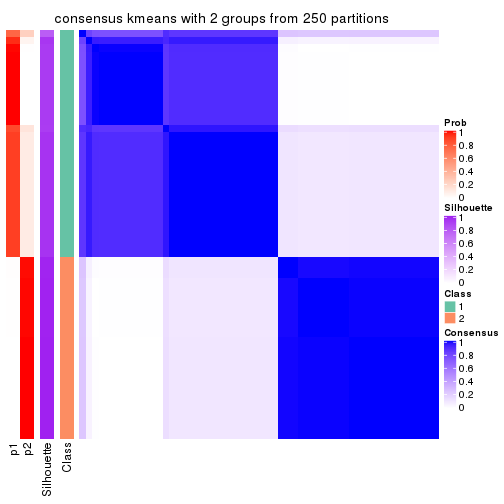
consensus_heatmap(res, k = 3)
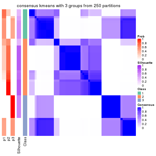
consensus_heatmap(res, k = 4)
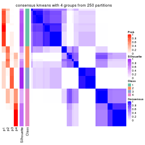
consensus_heatmap(res, k = 5)
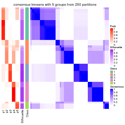
consensus_heatmap(res, k = 6)
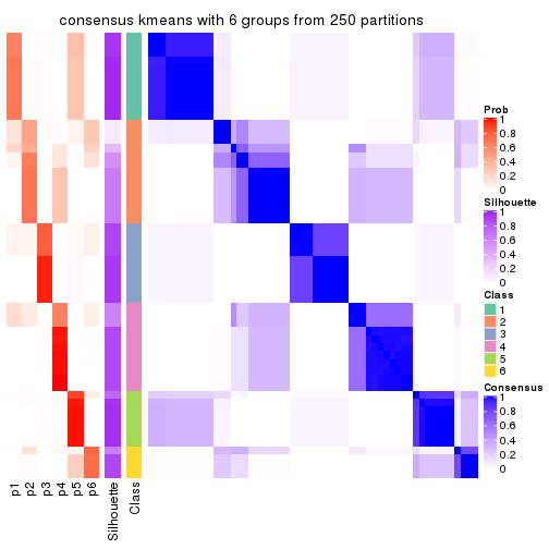
Heatmaps for the membership of samples in all partitions to see how consistent they are:
membership_heatmap(res, k = 2)
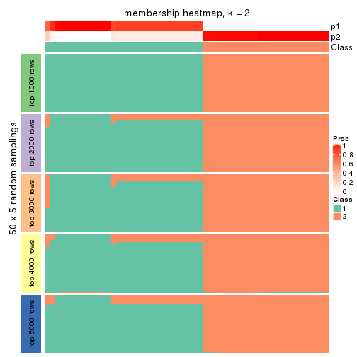
membership_heatmap(res, k = 3)
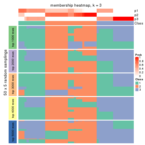
membership_heatmap(res, k = 4)
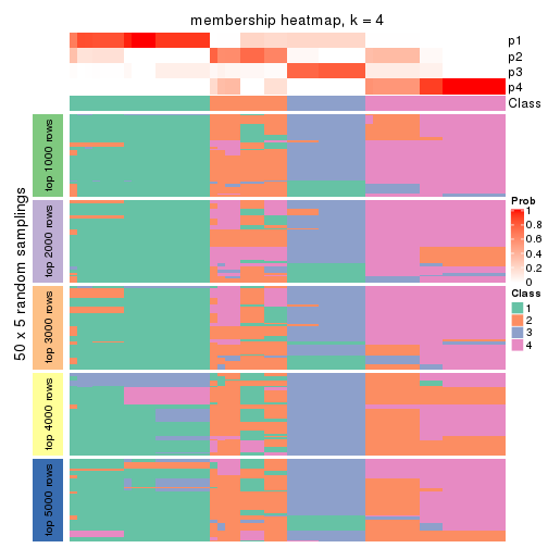
membership_heatmap(res, k = 5)
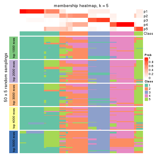
membership_heatmap(res, k = 6)
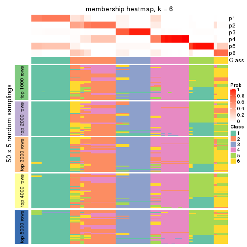
As soon as we have had the classes for columns, we can look for signatures which are significantly different between classes which can be candidate marks for certain classes. Following are the heatmaps for signatures.
Signature heatmaps where rows are scaled:
get_signatures(res, k = 2)
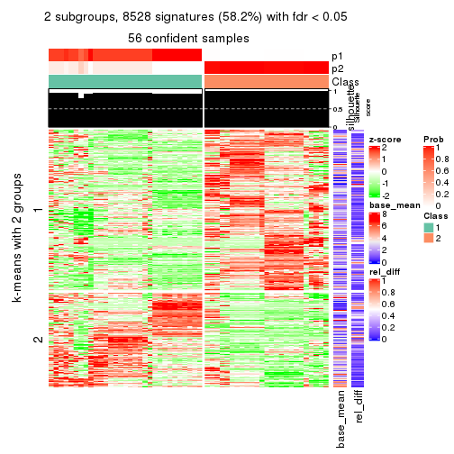
get_signatures(res, k = 3)
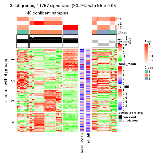
get_signatures(res, k = 4)
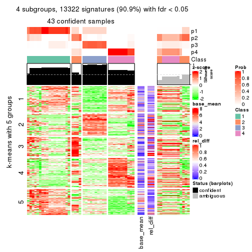
get_signatures(res, k = 5)
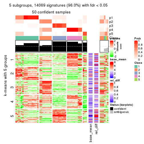
get_signatures(res, k = 6)
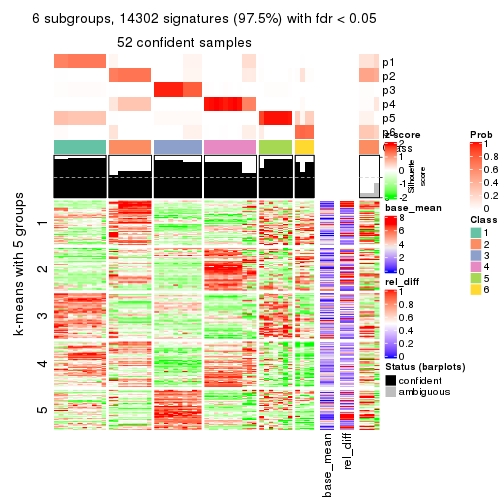
Signature heatmaps where rows are not scaled:
get_signatures(res, k = 2, scale_rows = FALSE)
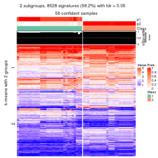
get_signatures(res, k = 3, scale_rows = FALSE)
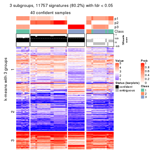
get_signatures(res, k = 4, scale_rows = FALSE)
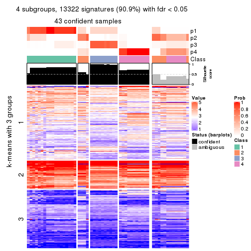
get_signatures(res, k = 5, scale_rows = FALSE)
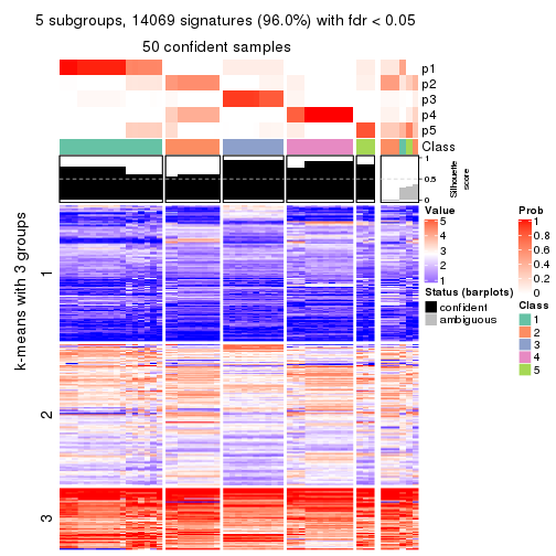
get_signatures(res, k = 6, scale_rows = FALSE)
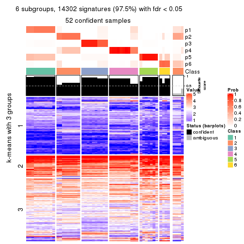
Compare the overlap of signatures from different k:
compare_signatures(res)
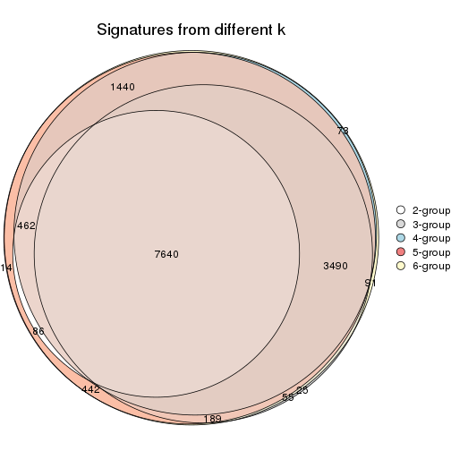
get_signature() returns a data frame invisibly. TO get the list of signatures, the function
call should be assigned to a variable explicitly. In following code, if plot argument is set
to FALSE, no heatmap is plotted while only the differential analysis is performed.
# code only for demonstration
tb = get_signature(res, k = ..., plot = FALSE)
An example of the output of tb is:
#> which_row fdr mean_1 mean_2 scaled_mean_1 scaled_mean_2 km
#> 1 38 0.042760348 8.373488 9.131774 -0.5533452 0.5164555 1
#> 2 40 0.018707592 7.106213 8.469186 -0.6173731 0.5762149 1
#> 3 55 0.019134737 10.221463 11.207825 -0.6159697 0.5749050 1
#> 4 59 0.006059896 5.921854 7.869574 -0.6899429 0.6439467 1
#> 5 60 0.018055526 8.928898 10.211722 -0.6204761 0.5791110 1
#> 6 98 0.009384629 15.714769 14.887706 0.6635654 -0.6193277 2
...
The columns in tb are:
which_row: row indices corresponding to the input matrix.fdr: FDR for the differential test. mean_x: The mean value in group x.scaled_mean_x: The mean value in group x after rows are scaled.km: Row groups if k-means clustering is applied to rows.UMAP plot which shows how samples are separated.
dimension_reduction(res, k = 2, method = "UMAP")
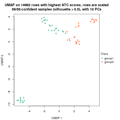
dimension_reduction(res, k = 3, method = "UMAP")
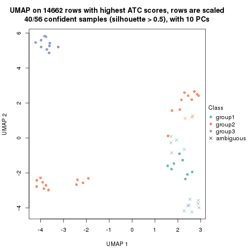
dimension_reduction(res, k = 4, method = "UMAP")
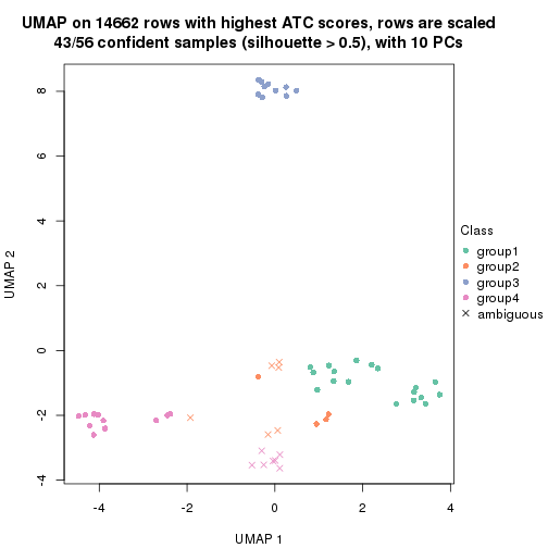
dimension_reduction(res, k = 5, method = "UMAP")
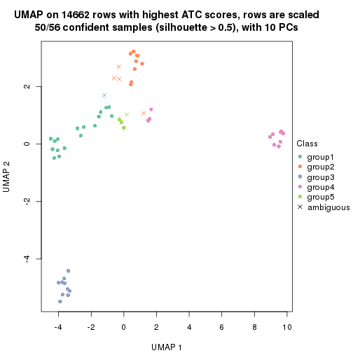
dimension_reduction(res, k = 6, method = "UMAP")

Following heatmap shows how subgroups are split when increasing k:
collect_classes(res)
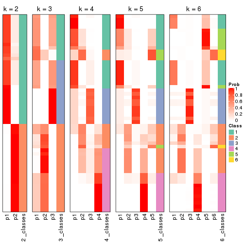
If matrix rows can be associated to genes, consider to use functional_enrichment(res,
...) to perform function enrichment for the signature genes. See this vignette for more detailed explanations.
The object with results only for a single top-value method and a single partition method can be extracted as:
res = res_list["ATC", "skmeans"]
# you can also extract it by
# res = res_list["ATC:skmeans"]
A summary of res and all the functions that can be applied to it:
res
#> A 'ConsensusPartition' object with k = 2, 3, 4, 5, 6.
#> On a matrix with 14662 rows and 56 columns.
#> Top rows (1000, 2000, 3000, 4000, 5000) are extracted by 'ATC' method.
#> Subgroups are detected by 'skmeans' method.
#> Performed in total 1250 partitions by row resampling.
#> Best k for subgroups seems to be 3.
#>
#> Following methods can be applied to this 'ConsensusPartition' object:
#> [1] "cola_report" "collect_classes" "collect_plots"
#> [4] "collect_stats" "colnames" "compare_signatures"
#> [7] "consensus_heatmap" "dimension_reduction" "functional_enrichment"
#> [10] "get_anno_col" "get_anno" "get_classes"
#> [13] "get_consensus" "get_matrix" "get_membership"
#> [16] "get_param" "get_signatures" "get_stats"
#> [19] "is_best_k" "is_stable_k" "membership_heatmap"
#> [22] "ncol" "nrow" "plot_ecdf"
#> [25] "rownames" "select_partition_number" "show"
#> [28] "suggest_best_k" "test_to_known_factors"
collect_plots() function collects all the plots made from res for all k (number of partitions)
into one single page to provide an easy and fast comparison between different k.
collect_plots(res)
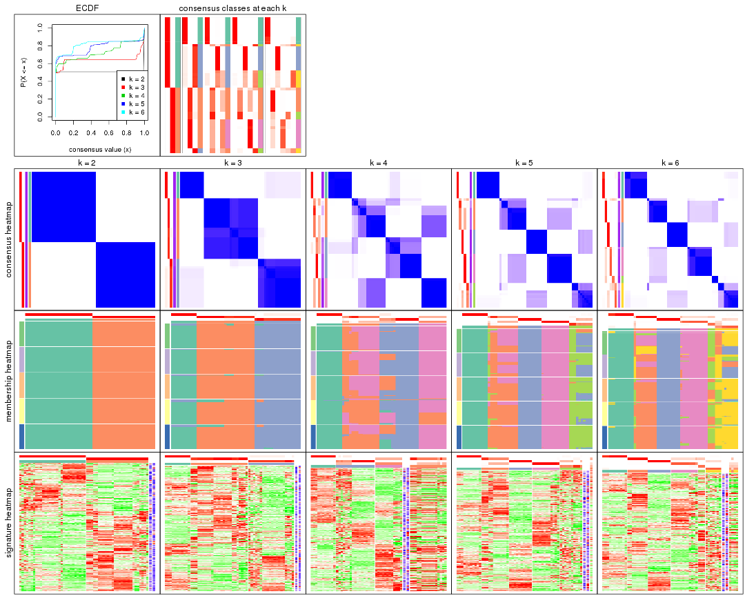
The plots are:
k and the heatmap of
predicted classes for each k.k.k.k.All the plots in panels can be made by individual functions and they are plotted later in this section.
select_partition_number() produces several plots showing different
statistics for choosing “optimized” k. There are following statistics:
k;k, the area increased is defined as \(A_k - A_{k-1}\).The detailed explanations of these statistics can be found in the cola vignette.
Generally speaking, lower PAC score, higher mean silhouette score or higher
concordance corresponds to better partition. Rand index and Jaccard index
measure how similar the current partition is compared to partition with k-1.
If they are too similar, we won't accept k is better than k-1.
select_partition_number(res)
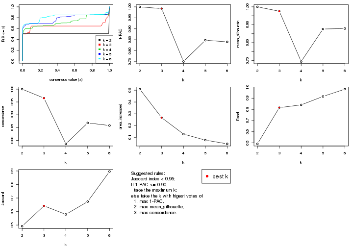
The numeric values for all these statistics can be obtained by get_stats().
get_stats(res)
#> k 1-PAC mean_silhouette concordance area_increased Rand Jaccard
#> 2 2 1.000 1.000 1.000 0.5089 0.492 0.492
#> 3 3 0.992 0.975 0.965 0.2668 0.816 0.642
#> 4 4 0.751 0.695 0.786 0.1277 0.840 0.579
#> 5 5 0.848 0.876 0.868 0.0761 0.916 0.673
#> 6 6 0.840 0.879 0.858 0.0446 0.981 0.896
suggest_best_k() suggests the best \(k\) based on these statistics. The rules are as follows:
suggest_best_k(res)
#> [1] 3
#> attr(,"optional")
#> [1] 2
There is also optional best \(k\) = 2 that is worth to check.
Following shows the table of the partitions (You need to click the show/hide
code output link to see it). The membership matrix (columns with name p*)
is inferred by
clue::cl_consensus()
function with the SE method. Basically the value in the membership matrix
represents the probability to belong to a certain group. The finall class
label for an item is determined with the group with highest probability it
belongs to.
In get_classes() function, the entropy is calculated from the membership
matrix and the silhouette score is calculated from the consensus matrix.
cbind(get_classes(res, k = 2), get_membership(res, k = 2))
#> class entropy silhouette p1 p2
#> SRR073723 1 0.0000 1.000 1.000 0.000
#> SRR073724 1 0.0000 1.000 1.000 0.000
#> SRR073725 1 0.0000 1.000 1.000 0.000
#> SRR073726 2 0.0000 1.000 0.000 1.000
#> SRR073727 1 0.0000 1.000 1.000 0.000
#> SRR073728 2 0.0000 1.000 0.000 1.000
#> SRR073729 2 0.0000 1.000 0.000 1.000
#> SRR073730 2 0.0000 1.000 0.000 1.000
#> SRR073731 2 0.0000 1.000 0.000 1.000
#> SRR073732 2 0.0000 1.000 0.000 1.000
#> SRR073733 2 0.0000 1.000 0.000 1.000
#> SRR073734 2 0.0000 1.000 0.000 1.000
#> SRR073735 2 0.0000 1.000 0.000 1.000
#> SRR073736 2 0.0000 1.000 0.000 1.000
#> SRR073737 2 0.0000 1.000 0.000 1.000
#> SRR073738 1 0.0000 1.000 1.000 0.000
#> SRR073739 1 0.0000 1.000 1.000 0.000
#> SRR073740 1 0.0000 1.000 1.000 0.000
#> SRR073741 1 0.0000 1.000 1.000 0.000
#> SRR073742 1 0.0000 1.000 1.000 0.000
#> SRR073743 1 0.0000 1.000 1.000 0.000
#> SRR073744 1 0.0000 1.000 1.000 0.000
#> SRR073745 1 0.0000 1.000 1.000 0.000
#> SRR073746 1 0.0000 1.000 1.000 0.000
#> SRR073747 1 0.0000 1.000 1.000 0.000
#> SRR073748 1 0.0000 1.000 1.000 0.000
#> SRR073749 1 0.0000 1.000 1.000 0.000
#> SRR073750 1 0.0000 1.000 1.000 0.000
#> SRR073751 1 0.0000 1.000 1.000 0.000
#> SRR073752 2 0.0000 1.000 0.000 1.000
#> SRR073753 2 0.0000 1.000 0.000 1.000
#> SRR073754 1 0.0000 1.000 1.000 0.000
#> SRR073755 2 0.0000 1.000 0.000 1.000
#> SRR073756 2 0.0000 1.000 0.000 1.000
#> SRR073758 2 0.0000 1.000 0.000 1.000
#> SRR073759 2 0.0000 1.000 0.000 1.000
#> SRR073760 2 0.0000 1.000 0.000 1.000
#> SRR073761 2 0.0000 1.000 0.000 1.000
#> SRR073763 2 0.0000 1.000 0.000 1.000
#> SRR073764 2 0.0000 1.000 0.000 1.000
#> SRR073765 2 0.0000 1.000 0.000 1.000
#> SRR073766 2 0.0000 1.000 0.000 1.000
#> SRR073767 2 0.0000 1.000 0.000 1.000
#> SRR073768 2 0.0000 1.000 0.000 1.000
#> SRR073769 1 0.0000 1.000 1.000 0.000
#> SRR073770 1 0.0000 1.000 1.000 0.000
#> SRR073771 1 0.0000 1.000 1.000 0.000
#> SRR073772 1 0.0000 1.000 1.000 0.000
#> SRR073773 1 0.0000 1.000 1.000 0.000
#> SRR073774 1 0.0000 1.000 1.000 0.000
#> SRR073775 1 0.0000 1.000 1.000 0.000
#> SRR073776 1 0.0000 1.000 1.000 0.000
#> SRR073777 1 0.0000 1.000 1.000 0.000
#> SRR073778 1 0.0000 1.000 1.000 0.000
#> SRR073779 2 0.0376 0.996 0.004 0.996
#> SRR073780 2 0.0000 1.000 0.000 1.000
cbind(get_classes(res, k = 3), get_membership(res, k = 3))
#> class entropy silhouette p1 p2 p3
#> SRR073723 3 0.263 0.980 0.084 0.000 0.916
#> SRR073724 3 0.296 0.970 0.100 0.000 0.900
#> SRR073725 3 0.263 0.980 0.084 0.000 0.916
#> SRR073726 2 0.236 0.963 0.000 0.928 0.072
#> SRR073727 3 0.288 0.973 0.096 0.000 0.904
#> SRR073728 2 0.263 0.956 0.000 0.916 0.084
#> SRR073729 2 0.263 0.956 0.000 0.916 0.084
#> SRR073730 2 0.263 0.956 0.000 0.916 0.084
#> SRR073731 2 0.175 0.974 0.000 0.952 0.048
#> SRR073732 2 0.175 0.974 0.000 0.952 0.048
#> SRR073733 2 0.175 0.974 0.000 0.952 0.048
#> SRR073734 2 0.175 0.974 0.000 0.952 0.048
#> SRR073735 2 0.175 0.974 0.000 0.952 0.048
#> SRR073736 2 0.175 0.974 0.000 0.952 0.048
#> SRR073737 2 0.175 0.974 0.000 0.952 0.048
#> SRR073738 3 0.288 0.973 0.096 0.000 0.904
#> SRR073739 1 0.000 1.000 1.000 0.000 0.000
#> SRR073740 1 0.000 1.000 1.000 0.000 0.000
#> SRR073741 1 0.000 1.000 1.000 0.000 0.000
#> SRR073742 1 0.000 1.000 1.000 0.000 0.000
#> SRR073743 1 0.000 1.000 1.000 0.000 0.000
#> SRR073744 1 0.000 1.000 1.000 0.000 0.000
#> SRR073745 1 0.000 1.000 1.000 0.000 0.000
#> SRR073746 1 0.000 1.000 1.000 0.000 0.000
#> SRR073747 1 0.000 1.000 1.000 0.000 0.000
#> SRR073748 1 0.000 1.000 1.000 0.000 0.000
#> SRR073749 1 0.000 1.000 1.000 0.000 0.000
#> SRR073750 3 0.288 0.973 0.096 0.000 0.904
#> SRR073751 3 0.207 0.964 0.060 0.000 0.940
#> SRR073752 2 0.175 0.974 0.000 0.952 0.048
#> SRR073753 2 0.175 0.974 0.000 0.952 0.048
#> SRR073754 3 0.000 0.911 0.000 0.000 1.000
#> SRR073755 2 0.000 0.974 0.000 1.000 0.000
#> SRR073756 2 0.000 0.974 0.000 1.000 0.000
#> SRR073758 2 0.000 0.974 0.000 1.000 0.000
#> SRR073759 2 0.000 0.974 0.000 1.000 0.000
#> SRR073760 2 0.000 0.974 0.000 1.000 0.000
#> SRR073761 2 0.000 0.974 0.000 1.000 0.000
#> SRR073763 2 0.000 0.974 0.000 1.000 0.000
#> SRR073764 2 0.000 0.974 0.000 1.000 0.000
#> SRR073765 2 0.000 0.974 0.000 1.000 0.000
#> SRR073766 2 0.000 0.974 0.000 1.000 0.000
#> SRR073767 2 0.000 0.974 0.000 1.000 0.000
#> SRR073768 2 0.000 0.974 0.000 1.000 0.000
#> SRR073769 3 0.263 0.980 0.084 0.000 0.916
#> SRR073770 3 0.263 0.980 0.084 0.000 0.916
#> SRR073771 3 0.263 0.980 0.084 0.000 0.916
#> SRR073772 3 0.263 0.980 0.084 0.000 0.916
#> SRR073773 3 0.263 0.980 0.084 0.000 0.916
#> SRR073774 3 0.263 0.980 0.084 0.000 0.916
#> SRR073775 3 0.263 0.980 0.084 0.000 0.916
#> SRR073776 3 0.263 0.980 0.084 0.000 0.916
#> SRR073777 3 0.263 0.980 0.084 0.000 0.916
#> SRR073778 3 0.263 0.980 0.084 0.000 0.916
#> SRR073779 3 0.000 0.911 0.000 0.000 1.000
#> SRR073780 3 0.000 0.911 0.000 0.000 1.000
cbind(get_classes(res, k = 4), get_membership(res, k = 4))
#> class entropy silhouette p1 p2 p3 p4
#> SRR073723 3 0.5038 0.7464 0.012 0.000 0.652 0.336
#> SRR073724 3 0.6824 0.6962 0.116 0.000 0.548 0.336
#> SRR073725 3 0.6764 0.7011 0.112 0.000 0.556 0.332
#> SRR073726 2 0.2266 0.3872 0.004 0.912 0.000 0.084
#> SRR073727 3 0.6824 0.6962 0.116 0.000 0.548 0.336
#> SRR073728 2 0.0817 0.3990 0.000 0.976 0.000 0.024
#> SRR073729 2 0.0817 0.3990 0.000 0.976 0.000 0.024
#> SRR073730 2 0.0817 0.3990 0.000 0.976 0.000 0.024
#> SRR073731 2 0.4564 0.0848 0.000 0.672 0.000 0.328
#> SRR073732 2 0.4564 0.0848 0.000 0.672 0.000 0.328
#> SRR073733 2 0.4564 0.0848 0.000 0.672 0.000 0.328
#> SRR073734 2 0.4564 0.0848 0.000 0.672 0.000 0.328
#> SRR073735 2 0.4564 0.0848 0.000 0.672 0.000 0.328
#> SRR073736 2 0.4564 0.0848 0.000 0.672 0.000 0.328
#> SRR073737 2 0.4564 0.0848 0.000 0.672 0.000 0.328
#> SRR073738 3 0.6824 0.6962 0.116 0.000 0.548 0.336
#> SRR073739 1 0.0336 0.9985 0.992 0.000 0.008 0.000
#> SRR073740 1 0.0336 0.9985 0.992 0.000 0.008 0.000
#> SRR073741 1 0.0336 0.9985 0.992 0.000 0.008 0.000
#> SRR073742 1 0.0336 0.9985 0.992 0.000 0.008 0.000
#> SRR073743 1 0.0336 0.9985 0.992 0.000 0.008 0.000
#> SRR073744 1 0.0336 0.9985 0.992 0.000 0.008 0.000
#> SRR073745 1 0.0336 0.9985 0.992 0.000 0.008 0.000
#> SRR073746 1 0.0336 0.9985 0.992 0.000 0.008 0.000
#> SRR073747 1 0.0188 0.9961 0.996 0.000 0.004 0.000
#> SRR073748 1 0.0188 0.9961 0.996 0.000 0.004 0.000
#> SRR073749 1 0.0188 0.9961 0.996 0.000 0.004 0.000
#> SRR073750 3 0.6809 0.6982 0.116 0.000 0.552 0.332
#> SRR073751 3 0.5464 0.7384 0.004 0.020 0.632 0.344
#> SRR073752 2 0.4543 0.0922 0.000 0.676 0.000 0.324
#> SRR073753 2 0.4543 0.0922 0.000 0.676 0.000 0.324
#> SRR073754 2 0.7106 -0.0127 0.008 0.488 0.100 0.404
#> SRR073755 4 0.4866 0.9992 0.000 0.404 0.000 0.596
#> SRR073756 4 0.4866 0.9992 0.000 0.404 0.000 0.596
#> SRR073758 4 0.4866 0.9992 0.000 0.404 0.000 0.596
#> SRR073759 4 0.4877 0.9907 0.000 0.408 0.000 0.592
#> SRR073760 4 0.4866 0.9992 0.000 0.404 0.000 0.596
#> SRR073761 4 0.4866 0.9992 0.000 0.404 0.000 0.596
#> SRR073763 4 0.4866 0.9992 0.000 0.404 0.000 0.596
#> SRR073764 4 0.4866 0.9992 0.000 0.404 0.000 0.596
#> SRR073765 4 0.4866 0.9992 0.000 0.404 0.000 0.596
#> SRR073766 4 0.4866 0.9992 0.000 0.404 0.000 0.596
#> SRR073767 4 0.4866 0.9992 0.000 0.404 0.000 0.596
#> SRR073768 4 0.4866 0.9992 0.000 0.404 0.000 0.596
#> SRR073769 3 0.0000 0.8335 0.000 0.000 1.000 0.000
#> SRR073770 3 0.0000 0.8335 0.000 0.000 1.000 0.000
#> SRR073771 3 0.0000 0.8335 0.000 0.000 1.000 0.000
#> SRR073772 3 0.0000 0.8335 0.000 0.000 1.000 0.000
#> SRR073773 3 0.0000 0.8335 0.000 0.000 1.000 0.000
#> SRR073774 3 0.0000 0.8335 0.000 0.000 1.000 0.000
#> SRR073775 3 0.0000 0.8335 0.000 0.000 1.000 0.000
#> SRR073776 3 0.0000 0.8335 0.000 0.000 1.000 0.000
#> SRR073777 3 0.0000 0.8335 0.000 0.000 1.000 0.000
#> SRR073778 3 0.0000 0.8335 0.000 0.000 1.000 0.000
#> SRR073779 2 0.5984 0.1479 0.008 0.560 0.028 0.404
#> SRR073780 2 0.5984 0.1479 0.008 0.560 0.028 0.404
cbind(get_classes(res, k = 5), get_membership(res, k = 5))
#> class entropy silhouette p1 p2 p3 p4 p5
#> SRR073723 5 0.4390 0.658 0.000 0.004 0.428 0.000 0.568
#> SRR073724 5 0.4977 0.748 0.040 0.000 0.356 0.000 0.604
#> SRR073725 5 0.4663 0.737 0.020 0.000 0.376 0.000 0.604
#> SRR073726 2 0.6537 0.415 0.000 0.404 0.000 0.196 0.400
#> SRR073727 5 0.4836 0.752 0.032 0.000 0.356 0.000 0.612
#> SRR073728 2 0.1549 0.572 0.000 0.944 0.000 0.016 0.040
#> SRR073729 2 0.1549 0.572 0.000 0.944 0.000 0.016 0.040
#> SRR073730 2 0.1549 0.572 0.000 0.944 0.000 0.016 0.040
#> SRR073731 2 0.4150 0.782 0.000 0.612 0.000 0.388 0.000
#> SRR073732 2 0.4150 0.782 0.000 0.612 0.000 0.388 0.000
#> SRR073733 2 0.4150 0.782 0.000 0.612 0.000 0.388 0.000
#> SRR073734 2 0.4150 0.782 0.000 0.612 0.000 0.388 0.000
#> SRR073735 2 0.4150 0.782 0.000 0.612 0.000 0.388 0.000
#> SRR073736 2 0.4150 0.782 0.000 0.612 0.000 0.388 0.000
#> SRR073737 2 0.4150 0.782 0.000 0.612 0.000 0.388 0.000
#> SRR073738 5 0.4794 0.754 0.032 0.000 0.344 0.000 0.624
#> SRR073739 1 0.0000 1.000 1.000 0.000 0.000 0.000 0.000
#> SRR073740 1 0.0000 1.000 1.000 0.000 0.000 0.000 0.000
#> SRR073741 1 0.0000 1.000 1.000 0.000 0.000 0.000 0.000
#> SRR073742 1 0.0000 1.000 1.000 0.000 0.000 0.000 0.000
#> SRR073743 1 0.0000 1.000 1.000 0.000 0.000 0.000 0.000
#> SRR073744 1 0.0000 1.000 1.000 0.000 0.000 0.000 0.000
#> SRR073745 1 0.0000 1.000 1.000 0.000 0.000 0.000 0.000
#> SRR073746 1 0.0000 1.000 1.000 0.000 0.000 0.000 0.000
#> SRR073747 1 0.0000 1.000 1.000 0.000 0.000 0.000 0.000
#> SRR073748 1 0.0000 1.000 1.000 0.000 0.000 0.000 0.000
#> SRR073749 1 0.0000 1.000 1.000 0.000 0.000 0.000 0.000
#> SRR073750 5 0.4921 0.748 0.036 0.000 0.360 0.000 0.604
#> SRR073751 5 0.4030 0.740 0.000 0.000 0.352 0.000 0.648
#> SRR073752 2 0.4126 0.781 0.000 0.620 0.000 0.380 0.000
#> SRR073753 2 0.4126 0.781 0.000 0.620 0.000 0.380 0.000
#> SRR073754 5 0.1410 0.612 0.000 0.060 0.000 0.000 0.940
#> SRR073755 4 0.0000 0.997 0.000 0.000 0.000 1.000 0.000
#> SRR073756 4 0.0000 0.997 0.000 0.000 0.000 1.000 0.000
#> SRR073758 4 0.0000 0.997 0.000 0.000 0.000 1.000 0.000
#> SRR073759 4 0.0771 0.966 0.000 0.020 0.000 0.976 0.004
#> SRR073760 4 0.0000 0.997 0.000 0.000 0.000 1.000 0.000
#> SRR073761 4 0.0000 0.997 0.000 0.000 0.000 1.000 0.000
#> SRR073763 4 0.0000 0.997 0.000 0.000 0.000 1.000 0.000
#> SRR073764 4 0.0000 0.997 0.000 0.000 0.000 1.000 0.000
#> SRR073765 4 0.0000 0.997 0.000 0.000 0.000 1.000 0.000
#> SRR073766 4 0.0000 0.997 0.000 0.000 0.000 1.000 0.000
#> SRR073767 4 0.0000 0.997 0.000 0.000 0.000 1.000 0.000
#> SRR073768 4 0.0000 0.997 0.000 0.000 0.000 1.000 0.000
#> SRR073769 3 0.0000 1.000 0.000 0.000 1.000 0.000 0.000
#> SRR073770 3 0.0000 1.000 0.000 0.000 1.000 0.000 0.000
#> SRR073771 3 0.0000 1.000 0.000 0.000 1.000 0.000 0.000
#> SRR073772 3 0.0000 1.000 0.000 0.000 1.000 0.000 0.000
#> SRR073773 3 0.0000 1.000 0.000 0.000 1.000 0.000 0.000
#> SRR073774 3 0.0000 1.000 0.000 0.000 1.000 0.000 0.000
#> SRR073775 3 0.0000 1.000 0.000 0.000 1.000 0.000 0.000
#> SRR073776 3 0.0000 1.000 0.000 0.000 1.000 0.000 0.000
#> SRR073777 3 0.0000 1.000 0.000 0.000 1.000 0.000 0.000
#> SRR073778 3 0.0000 1.000 0.000 0.000 1.000 0.000 0.000
#> SRR073779 5 0.1410 0.612 0.000 0.060 0.000 0.000 0.940
#> SRR073780 5 0.1410 0.612 0.000 0.060 0.000 0.000 0.940
cbind(get_classes(res, k = 6), get_membership(res, k = 6))
#> class entropy silhouette p1 p2 p3 p4 p5 p6
#> SRR073723 6 0.316 0.732 0.000 0.000 0.232 0.000 0.004 0.764
#> SRR073724 6 0.322 0.763 0.020 0.000 0.188 0.000 0.000 0.792
#> SRR073725 6 0.314 0.760 0.012 0.000 0.200 0.000 0.000 0.788
#> SRR073726 2 0.761 -0.110 0.000 0.312 0.000 0.184 0.292 0.212
#> SRR073727 6 0.322 0.763 0.020 0.000 0.188 0.000 0.000 0.792
#> SRR073728 5 0.347 1.000 0.000 0.284 0.000 0.000 0.712 0.004
#> SRR073729 5 0.347 1.000 0.000 0.284 0.000 0.000 0.712 0.004
#> SRR073730 5 0.347 1.000 0.000 0.284 0.000 0.000 0.712 0.004
#> SRR073731 2 0.026 0.885 0.000 0.992 0.000 0.008 0.000 0.000
#> SRR073732 2 0.026 0.885 0.000 0.992 0.000 0.008 0.000 0.000
#> SRR073733 2 0.026 0.885 0.000 0.992 0.000 0.008 0.000 0.000
#> SRR073734 2 0.026 0.885 0.000 0.992 0.000 0.008 0.000 0.000
#> SRR073735 2 0.026 0.885 0.000 0.992 0.000 0.008 0.000 0.000
#> SRR073736 2 0.026 0.885 0.000 0.992 0.000 0.008 0.000 0.000
#> SRR073737 2 0.026 0.885 0.000 0.992 0.000 0.008 0.000 0.000
#> SRR073738 6 0.322 0.763 0.020 0.000 0.188 0.000 0.000 0.792
#> SRR073739 1 0.000 0.981 1.000 0.000 0.000 0.000 0.000 0.000
#> SRR073740 1 0.000 0.981 1.000 0.000 0.000 0.000 0.000 0.000
#> SRR073741 1 0.000 0.981 1.000 0.000 0.000 0.000 0.000 0.000
#> SRR073742 1 0.000 0.981 1.000 0.000 0.000 0.000 0.000 0.000
#> SRR073743 1 0.000 0.981 1.000 0.000 0.000 0.000 0.000 0.000
#> SRR073744 1 0.000 0.981 1.000 0.000 0.000 0.000 0.000 0.000
#> SRR073745 1 0.000 0.981 1.000 0.000 0.000 0.000 0.000 0.000
#> SRR073746 1 0.000 0.981 1.000 0.000 0.000 0.000 0.000 0.000
#> SRR073747 1 0.120 0.949 0.944 0.000 0.000 0.000 0.000 0.056
#> SRR073748 1 0.127 0.946 0.940 0.000 0.000 0.000 0.000 0.060
#> SRR073749 1 0.127 0.946 0.940 0.000 0.000 0.000 0.000 0.060
#> SRR073750 6 0.325 0.762 0.020 0.000 0.192 0.000 0.000 0.788
#> SRR073751 6 0.346 0.740 0.000 0.000 0.220 0.000 0.020 0.760
#> SRR073752 2 0.026 0.870 0.000 0.992 0.000 0.008 0.000 0.000
#> SRR073753 2 0.026 0.870 0.000 0.992 0.000 0.008 0.000 0.000
#> SRR073754 6 0.549 0.384 0.000 0.000 0.000 0.180 0.260 0.560
#> SRR073755 4 0.349 0.945 0.000 0.184 0.000 0.780 0.036 0.000
#> SRR073756 4 0.349 0.945 0.000 0.184 0.000 0.780 0.036 0.000
#> SRR073758 4 0.349 0.945 0.000 0.184 0.000 0.780 0.036 0.000
#> SRR073759 4 0.447 0.701 0.000 0.356 0.000 0.604 0.040 0.000
#> SRR073760 4 0.270 0.965 0.000 0.188 0.000 0.812 0.000 0.000
#> SRR073761 4 0.270 0.965 0.000 0.188 0.000 0.812 0.000 0.000
#> SRR073763 4 0.270 0.965 0.000 0.188 0.000 0.812 0.000 0.000
#> SRR073764 4 0.270 0.965 0.000 0.188 0.000 0.812 0.000 0.000
#> SRR073765 4 0.270 0.965 0.000 0.188 0.000 0.812 0.000 0.000
#> SRR073766 4 0.270 0.965 0.000 0.188 0.000 0.812 0.000 0.000
#> SRR073767 4 0.270 0.965 0.000 0.188 0.000 0.812 0.000 0.000
#> SRR073768 4 0.270 0.965 0.000 0.188 0.000 0.812 0.000 0.000
#> SRR073769 3 0.000 1.000 0.000 0.000 1.000 0.000 0.000 0.000
#> SRR073770 3 0.000 1.000 0.000 0.000 1.000 0.000 0.000 0.000
#> SRR073771 3 0.000 1.000 0.000 0.000 1.000 0.000 0.000 0.000
#> SRR073772 3 0.000 1.000 0.000 0.000 1.000 0.000 0.000 0.000
#> SRR073773 3 0.000 1.000 0.000 0.000 1.000 0.000 0.000 0.000
#> SRR073774 3 0.000 1.000 0.000 0.000 1.000 0.000 0.000 0.000
#> SRR073775 3 0.000 1.000 0.000 0.000 1.000 0.000 0.000 0.000
#> SRR073776 3 0.000 1.000 0.000 0.000 1.000 0.000 0.000 0.000
#> SRR073777 3 0.000 1.000 0.000 0.000 1.000 0.000 0.000 0.000
#> SRR073778 3 0.000 1.000 0.000 0.000 1.000 0.000 0.000 0.000
#> SRR073779 6 0.549 0.384 0.000 0.000 0.000 0.180 0.260 0.560
#> SRR073780 6 0.549 0.384 0.000 0.000 0.000 0.180 0.260 0.560
Heatmaps for the consensus matrix. It visualizes the probability of two samples to be in a same group.
consensus_heatmap(res, k = 2)
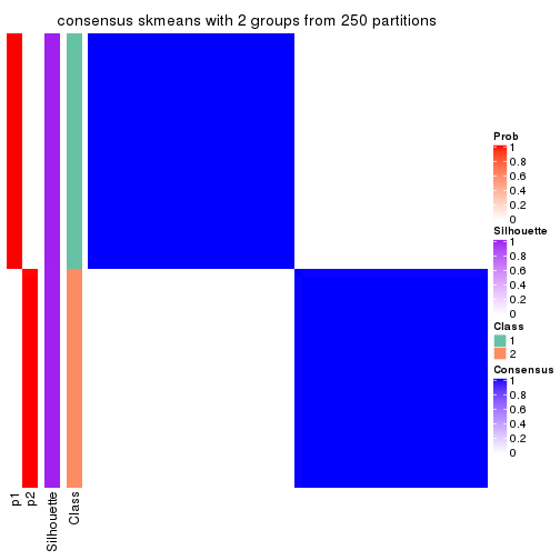
consensus_heatmap(res, k = 3)
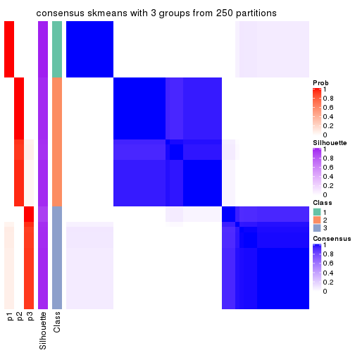
consensus_heatmap(res, k = 4)
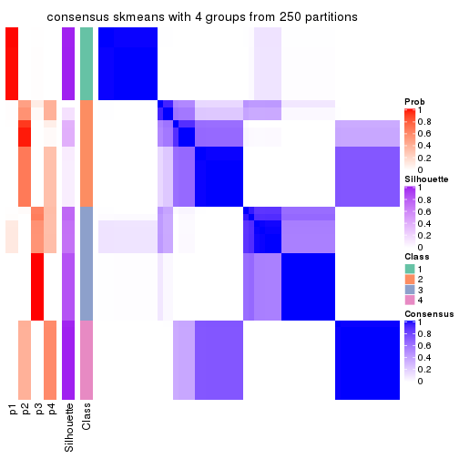
consensus_heatmap(res, k = 5)
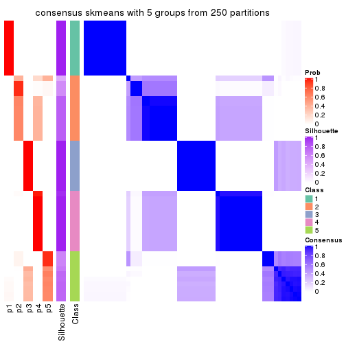
consensus_heatmap(res, k = 6)
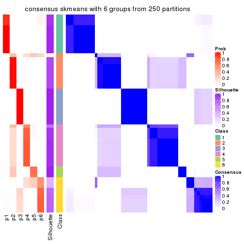
Heatmaps for the membership of samples in all partitions to see how consistent they are:
membership_heatmap(res, k = 2)

membership_heatmap(res, k = 3)
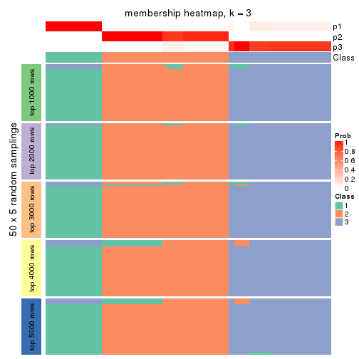
membership_heatmap(res, k = 4)
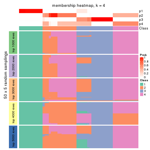
membership_heatmap(res, k = 5)
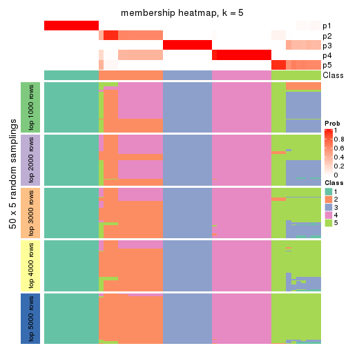
membership_heatmap(res, k = 6)
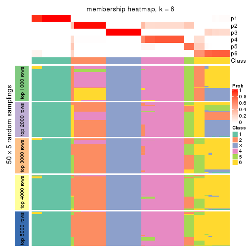
As soon as we have had the classes for columns, we can look for signatures which are significantly different between classes which can be candidate marks for certain classes. Following are the heatmaps for signatures.
Signature heatmaps where rows are scaled:
get_signatures(res, k = 2)

get_signatures(res, k = 3)
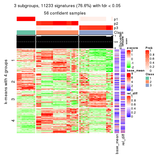
get_signatures(res, k = 4)
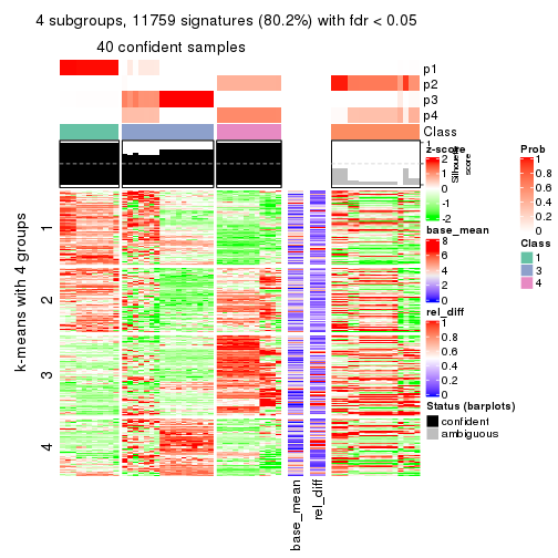
get_signatures(res, k = 5)
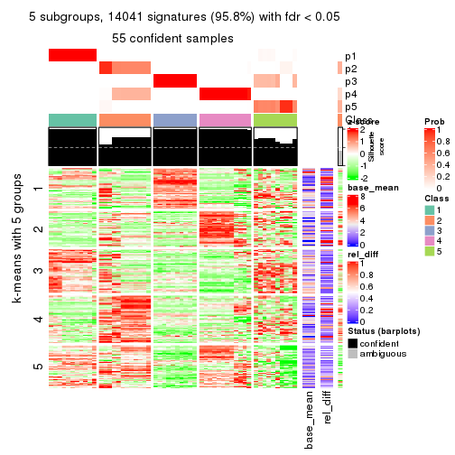
get_signatures(res, k = 6)
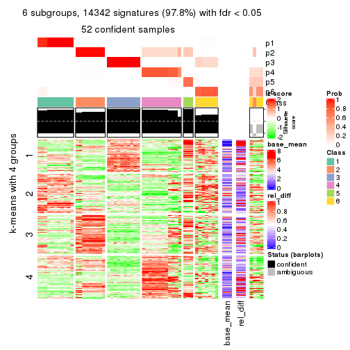
Signature heatmaps where rows are not scaled:
get_signatures(res, k = 2, scale_rows = FALSE)
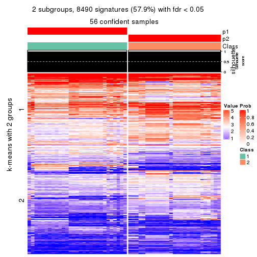
get_signatures(res, k = 3, scale_rows = FALSE)
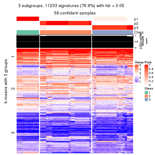
get_signatures(res, k = 4, scale_rows = FALSE)
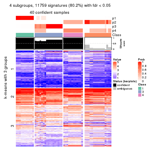
get_signatures(res, k = 5, scale_rows = FALSE)
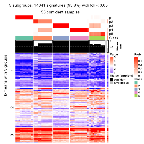
get_signatures(res, k = 6, scale_rows = FALSE)
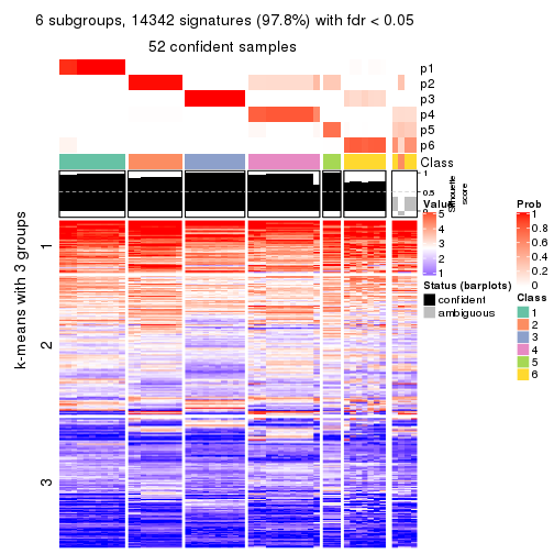
Compare the overlap of signatures from different k:
compare_signatures(res)
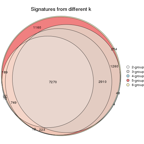
get_signature() returns a data frame invisibly. TO get the list of signatures, the function
call should be assigned to a variable explicitly. In following code, if plot argument is set
to FALSE, no heatmap is plotted while only the differential analysis is performed.
# code only for demonstration
tb = get_signature(res, k = ..., plot = FALSE)
An example of the output of tb is:
#> which_row fdr mean_1 mean_2 scaled_mean_1 scaled_mean_2 km
#> 1 38 0.042760348 8.373488 9.131774 -0.5533452 0.5164555 1
#> 2 40 0.018707592 7.106213 8.469186 -0.6173731 0.5762149 1
#> 3 55 0.019134737 10.221463 11.207825 -0.6159697 0.5749050 1
#> 4 59 0.006059896 5.921854 7.869574 -0.6899429 0.6439467 1
#> 5 60 0.018055526 8.928898 10.211722 -0.6204761 0.5791110 1
#> 6 98 0.009384629 15.714769 14.887706 0.6635654 -0.6193277 2
...
The columns in tb are:
which_row: row indices corresponding to the input matrix.fdr: FDR for the differential test. mean_x: The mean value in group x.scaled_mean_x: The mean value in group x after rows are scaled.km: Row groups if k-means clustering is applied to rows.UMAP plot which shows how samples are separated.
dimension_reduction(res, k = 2, method = "UMAP")
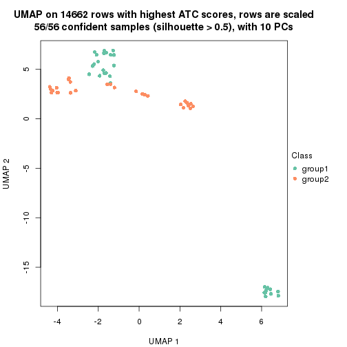
dimension_reduction(res, k = 3, method = "UMAP")
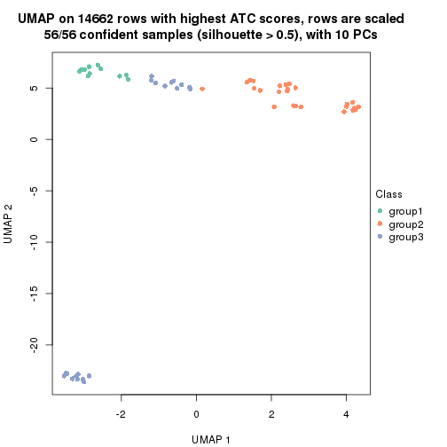
dimension_reduction(res, k = 4, method = "UMAP")
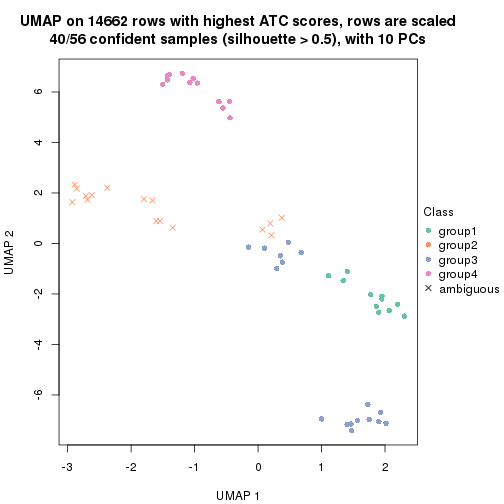
dimension_reduction(res, k = 5, method = "UMAP")
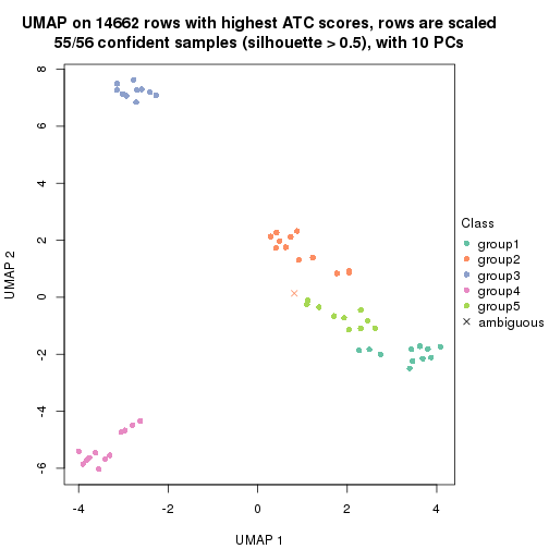
dimension_reduction(res, k = 6, method = "UMAP")
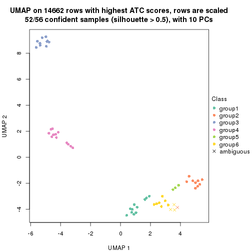
Following heatmap shows how subgroups are split when increasing k:
collect_classes(res)
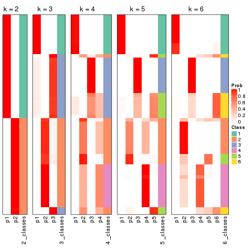
If matrix rows can be associated to genes, consider to use functional_enrichment(res,
...) to perform function enrichment for the signature genes. See this vignette for more detailed explanations.
The object with results only for a single top-value method and a single partition method can be extracted as:
res = res_list["ATC", "pam"]
# you can also extract it by
# res = res_list["ATC:pam"]
A summary of res and all the functions that can be applied to it:
res
#> A 'ConsensusPartition' object with k = 2, 3, 4, 5, 6.
#> On a matrix with 14662 rows and 56 columns.
#> Top rows (1000, 2000, 3000, 4000, 5000) are extracted by 'ATC' method.
#> Subgroups are detected by 'pam' method.
#> Performed in total 1250 partitions by row resampling.
#> Best k for subgroups seems to be 6.
#>
#> Following methods can be applied to this 'ConsensusPartition' object:
#> [1] "cola_report" "collect_classes" "collect_plots"
#> [4] "collect_stats" "colnames" "compare_signatures"
#> [7] "consensus_heatmap" "dimension_reduction" "functional_enrichment"
#> [10] "get_anno_col" "get_anno" "get_classes"
#> [13] "get_consensus" "get_matrix" "get_membership"
#> [16] "get_param" "get_signatures" "get_stats"
#> [19] "is_best_k" "is_stable_k" "membership_heatmap"
#> [22] "ncol" "nrow" "plot_ecdf"
#> [25] "rownames" "select_partition_number" "show"
#> [28] "suggest_best_k" "test_to_known_factors"
collect_plots() function collects all the plots made from res for all k (number of partitions)
into one single page to provide an easy and fast comparison between different k.
collect_plots(res)
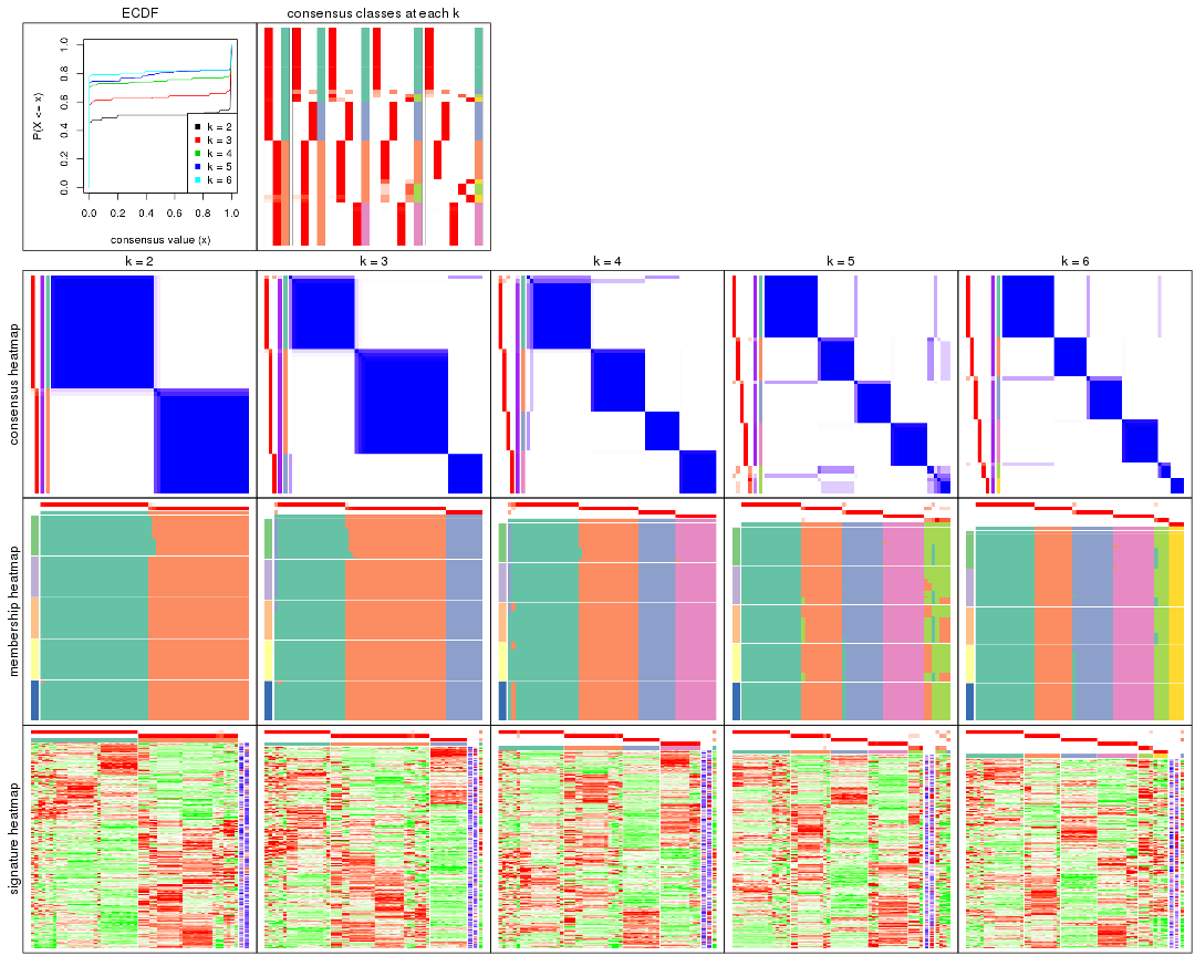
The plots are:
k and the heatmap of
predicted classes for each k.k.k.k.All the plots in panels can be made by individual functions and they are plotted later in this section.
select_partition_number() produces several plots showing different
statistics for choosing “optimized” k. There are following statistics:
k;k, the area increased is defined as \(A_k - A_{k-1}\).The detailed explanations of these statistics can be found in the cola vignette.
Generally speaking, lower PAC score, higher mean silhouette score or higher
concordance corresponds to better partition. Rand index and Jaccard index
measure how similar the current partition is compared to partition with k-1.
If they are too similar, we won't accept k is better than k-1.
select_partition_number(res)
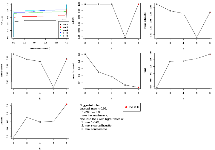
The numeric values for all these statistics can be obtained by get_stats().
get_stats(res)
#> k 1-PAC mean_silhouette concordance area_increased Rand Jaccard
#> 2 2 1.000 0.989 0.995 0.5083 0.492 0.492
#> 3 3 1.000 0.970 0.988 0.2499 0.877 0.749
#> 4 4 1.000 0.962 0.986 0.1787 0.886 0.690
#> 5 5 0.949 0.892 0.953 0.0574 0.919 0.696
#> 6 6 1.000 0.965 0.989 0.0235 0.984 0.919
suggest_best_k() suggests the best \(k\) based on these statistics. The rules are as follows:
suggest_best_k(res)
#> [1] 6
#> attr(,"optional")
#> [1] 2 3 4 5
There is also optional best \(k\) = 2 3 4 5 that is worth to check.
Following shows the table of the partitions (You need to click the show/hide
code output link to see it). The membership matrix (columns with name p*)
is inferred by
clue::cl_consensus()
function with the SE method. Basically the value in the membership matrix
represents the probability to belong to a certain group. The finall class
label for an item is determined with the group with highest probability it
belongs to.
In get_classes() function, the entropy is calculated from the membership
matrix and the silhouette score is calculated from the consensus matrix.
cbind(get_classes(res, k = 2), get_membership(res, k = 2))
#> class entropy silhouette p1 p2
#> SRR073723 1 0.0000 1.000 1.000 0.000
#> SRR073724 1 0.0000 1.000 1.000 0.000
#> SRR073725 1 0.0000 1.000 1.000 0.000
#> SRR073726 2 0.0000 0.989 0.000 1.000
#> SRR073727 1 0.0000 1.000 1.000 0.000
#> SRR073728 2 0.0000 0.989 0.000 1.000
#> SRR073729 2 0.0000 0.989 0.000 1.000
#> SRR073730 2 0.0000 0.989 0.000 1.000
#> SRR073731 2 0.0000 0.989 0.000 1.000
#> SRR073732 2 0.0000 0.989 0.000 1.000
#> SRR073733 2 0.0000 0.989 0.000 1.000
#> SRR073734 2 0.0000 0.989 0.000 1.000
#> SRR073735 2 0.0000 0.989 0.000 1.000
#> SRR073736 2 0.0000 0.989 0.000 1.000
#> SRR073737 2 0.0000 0.989 0.000 1.000
#> SRR073738 1 0.0000 1.000 1.000 0.000
#> SRR073739 1 0.0000 1.000 1.000 0.000
#> SRR073740 1 0.0000 1.000 1.000 0.000
#> SRR073741 1 0.0000 1.000 1.000 0.000
#> SRR073742 1 0.0000 1.000 1.000 0.000
#> SRR073743 1 0.0000 1.000 1.000 0.000
#> SRR073744 1 0.0000 1.000 1.000 0.000
#> SRR073745 1 0.0000 1.000 1.000 0.000
#> SRR073746 1 0.0000 1.000 1.000 0.000
#> SRR073747 1 0.0000 1.000 1.000 0.000
#> SRR073748 1 0.0000 1.000 1.000 0.000
#> SRR073749 1 0.0000 1.000 1.000 0.000
#> SRR073750 1 0.0000 1.000 1.000 0.000
#> SRR073751 1 0.0000 1.000 1.000 0.000
#> SRR073752 2 0.0000 0.989 0.000 1.000
#> SRR073753 2 0.0000 0.989 0.000 1.000
#> SRR073754 1 0.0938 0.988 0.988 0.012
#> SRR073755 2 0.0000 0.989 0.000 1.000
#> SRR073756 2 0.0000 0.989 0.000 1.000
#> SRR073758 2 0.0000 0.989 0.000 1.000
#> SRR073759 2 0.0000 0.989 0.000 1.000
#> SRR073760 2 0.0000 0.989 0.000 1.000
#> SRR073761 2 0.0000 0.989 0.000 1.000
#> SRR073763 2 0.0000 0.989 0.000 1.000
#> SRR073764 2 0.0000 0.989 0.000 1.000
#> SRR073765 2 0.0000 0.989 0.000 1.000
#> SRR073766 2 0.0000 0.989 0.000 1.000
#> SRR073767 2 0.0000 0.989 0.000 1.000
#> SRR073768 2 0.0000 0.989 0.000 1.000
#> SRR073769 1 0.0000 1.000 1.000 0.000
#> SRR073770 1 0.0000 1.000 1.000 0.000
#> SRR073771 1 0.0000 1.000 1.000 0.000
#> SRR073772 1 0.0000 1.000 1.000 0.000
#> SRR073773 1 0.0000 1.000 1.000 0.000
#> SRR073774 1 0.0000 1.000 1.000 0.000
#> SRR073775 1 0.0000 1.000 1.000 0.000
#> SRR073776 1 0.0000 1.000 1.000 0.000
#> SRR073777 1 0.0000 1.000 1.000 0.000
#> SRR073778 1 0.0000 1.000 1.000 0.000
#> SRR073779 2 0.7056 0.768 0.192 0.808
#> SRR073780 2 0.4161 0.907 0.084 0.916
cbind(get_classes(res, k = 3), get_membership(res, k = 3))
#> class entropy silhouette p1 p2 p3
#> SRR073723 1 0.0000 0.974 1.000 0.000 0.00
#> SRR073724 1 0.0000 0.974 1.000 0.000 0.00
#> SRR073725 1 0.6244 0.213 0.560 0.000 0.44
#> SRR073726 2 0.0000 0.992 0.000 1.000 0.00
#> SRR073727 1 0.0000 0.974 1.000 0.000 0.00
#> SRR073728 2 0.0000 0.992 0.000 1.000 0.00
#> SRR073729 2 0.0000 0.992 0.000 1.000 0.00
#> SRR073730 2 0.0424 0.984 0.008 0.992 0.00
#> SRR073731 2 0.0000 0.992 0.000 1.000 0.00
#> SRR073732 2 0.0000 0.992 0.000 1.000 0.00
#> SRR073733 2 0.0000 0.992 0.000 1.000 0.00
#> SRR073734 2 0.0000 0.992 0.000 1.000 0.00
#> SRR073735 2 0.0000 0.992 0.000 1.000 0.00
#> SRR073736 2 0.0000 0.992 0.000 1.000 0.00
#> SRR073737 2 0.0000 0.992 0.000 1.000 0.00
#> SRR073738 1 0.0000 0.974 1.000 0.000 0.00
#> SRR073739 1 0.0000 0.974 1.000 0.000 0.00
#> SRR073740 1 0.0000 0.974 1.000 0.000 0.00
#> SRR073741 1 0.0000 0.974 1.000 0.000 0.00
#> SRR073742 1 0.0000 0.974 1.000 0.000 0.00
#> SRR073743 1 0.0000 0.974 1.000 0.000 0.00
#> SRR073744 1 0.0000 0.974 1.000 0.000 0.00
#> SRR073745 1 0.0000 0.974 1.000 0.000 0.00
#> SRR073746 1 0.0000 0.974 1.000 0.000 0.00
#> SRR073747 1 0.0000 0.974 1.000 0.000 0.00
#> SRR073748 1 0.0000 0.974 1.000 0.000 0.00
#> SRR073749 1 0.0000 0.974 1.000 0.000 0.00
#> SRR073750 1 0.0000 0.974 1.000 0.000 0.00
#> SRR073751 1 0.0000 0.974 1.000 0.000 0.00
#> SRR073752 2 0.0000 0.992 0.000 1.000 0.00
#> SRR073753 2 0.0000 0.992 0.000 1.000 0.00
#> SRR073754 1 0.0592 0.961 0.988 0.012 0.00
#> SRR073755 2 0.0000 0.992 0.000 1.000 0.00
#> SRR073756 2 0.0000 0.992 0.000 1.000 0.00
#> SRR073758 2 0.0000 0.992 0.000 1.000 0.00
#> SRR073759 2 0.0000 0.992 0.000 1.000 0.00
#> SRR073760 2 0.0000 0.992 0.000 1.000 0.00
#> SRR073761 2 0.0000 0.992 0.000 1.000 0.00
#> SRR073763 2 0.0000 0.992 0.000 1.000 0.00
#> SRR073764 2 0.0000 0.992 0.000 1.000 0.00
#> SRR073765 2 0.0000 0.992 0.000 1.000 0.00
#> SRR073766 2 0.0000 0.992 0.000 1.000 0.00
#> SRR073767 2 0.0000 0.992 0.000 1.000 0.00
#> SRR073768 2 0.0000 0.992 0.000 1.000 0.00
#> SRR073769 3 0.0000 1.000 0.000 0.000 1.00
#> SRR073770 3 0.0000 1.000 0.000 0.000 1.00
#> SRR073771 3 0.0000 1.000 0.000 0.000 1.00
#> SRR073772 3 0.0000 1.000 0.000 0.000 1.00
#> SRR073773 3 0.0000 1.000 0.000 0.000 1.00
#> SRR073774 3 0.0000 1.000 0.000 0.000 1.00
#> SRR073775 3 0.0000 1.000 0.000 0.000 1.00
#> SRR073776 3 0.0000 1.000 0.000 0.000 1.00
#> SRR073777 3 0.0000 1.000 0.000 0.000 1.00
#> SRR073778 3 0.0000 1.000 0.000 0.000 1.00
#> SRR073779 2 0.3879 0.819 0.152 0.848 0.00
#> SRR073780 2 0.1411 0.956 0.036 0.964 0.00
cbind(get_classes(res, k = 4), get_membership(res, k = 4))
#> class entropy silhouette p1 p2 p3 p4
#> SRR073723 1 0.0000 0.957 1.000 0.000 0.000 0.000
#> SRR073724 1 0.0000 0.957 1.000 0.000 0.000 0.000
#> SRR073725 1 0.4967 0.173 0.548 0.000 0.452 0.000
#> SRR073726 2 0.0000 0.996 0.000 1.000 0.000 0.000
#> SRR073727 1 0.0000 0.957 1.000 0.000 0.000 0.000
#> SRR073728 2 0.0000 0.996 0.000 1.000 0.000 0.000
#> SRR073729 2 0.0000 0.996 0.000 1.000 0.000 0.000
#> SRR073730 2 0.0000 0.996 0.000 1.000 0.000 0.000
#> SRR073731 2 0.0000 0.996 0.000 1.000 0.000 0.000
#> SRR073732 2 0.0000 0.996 0.000 1.000 0.000 0.000
#> SRR073733 2 0.0000 0.996 0.000 1.000 0.000 0.000
#> SRR073734 2 0.0000 0.996 0.000 1.000 0.000 0.000
#> SRR073735 2 0.0000 0.996 0.000 1.000 0.000 0.000
#> SRR073736 2 0.0000 0.996 0.000 1.000 0.000 0.000
#> SRR073737 2 0.0000 0.996 0.000 1.000 0.000 0.000
#> SRR073738 1 0.0000 0.957 1.000 0.000 0.000 0.000
#> SRR073739 1 0.0000 0.957 1.000 0.000 0.000 0.000
#> SRR073740 1 0.0000 0.957 1.000 0.000 0.000 0.000
#> SRR073741 1 0.0000 0.957 1.000 0.000 0.000 0.000
#> SRR073742 1 0.0000 0.957 1.000 0.000 0.000 0.000
#> SRR073743 1 0.0000 0.957 1.000 0.000 0.000 0.000
#> SRR073744 1 0.0000 0.957 1.000 0.000 0.000 0.000
#> SRR073745 1 0.0000 0.957 1.000 0.000 0.000 0.000
#> SRR073746 1 0.0000 0.957 1.000 0.000 0.000 0.000
#> SRR073747 1 0.0000 0.957 1.000 0.000 0.000 0.000
#> SRR073748 1 0.0000 0.957 1.000 0.000 0.000 0.000
#> SRR073749 1 0.0000 0.957 1.000 0.000 0.000 0.000
#> SRR073750 1 0.0000 0.957 1.000 0.000 0.000 0.000
#> SRR073751 1 0.0000 0.957 1.000 0.000 0.000 0.000
#> SRR073752 2 0.0000 0.996 0.000 1.000 0.000 0.000
#> SRR073753 2 0.0000 0.996 0.000 1.000 0.000 0.000
#> SRR073754 1 0.4277 0.598 0.720 0.280 0.000 0.000
#> SRR073755 4 0.0000 0.998 0.000 0.000 0.000 1.000
#> SRR073756 4 0.0592 0.982 0.000 0.016 0.000 0.984
#> SRR073758 4 0.0000 0.998 0.000 0.000 0.000 1.000
#> SRR073759 2 0.0000 0.996 0.000 1.000 0.000 0.000
#> SRR073760 4 0.0000 0.998 0.000 0.000 0.000 1.000
#> SRR073761 4 0.0000 0.998 0.000 0.000 0.000 1.000
#> SRR073763 4 0.0000 0.998 0.000 0.000 0.000 1.000
#> SRR073764 4 0.0000 0.998 0.000 0.000 0.000 1.000
#> SRR073765 4 0.0000 0.998 0.000 0.000 0.000 1.000
#> SRR073766 4 0.0000 0.998 0.000 0.000 0.000 1.000
#> SRR073767 4 0.0000 0.998 0.000 0.000 0.000 1.000
#> SRR073768 4 0.0000 0.998 0.000 0.000 0.000 1.000
#> SRR073769 3 0.0000 1.000 0.000 0.000 1.000 0.000
#> SRR073770 3 0.0000 1.000 0.000 0.000 1.000 0.000
#> SRR073771 3 0.0000 1.000 0.000 0.000 1.000 0.000
#> SRR073772 3 0.0000 1.000 0.000 0.000 1.000 0.000
#> SRR073773 3 0.0000 1.000 0.000 0.000 1.000 0.000
#> SRR073774 3 0.0000 1.000 0.000 0.000 1.000 0.000
#> SRR073775 3 0.0000 1.000 0.000 0.000 1.000 0.000
#> SRR073776 3 0.0000 1.000 0.000 0.000 1.000 0.000
#> SRR073777 3 0.0000 1.000 0.000 0.000 1.000 0.000
#> SRR073778 3 0.0000 1.000 0.000 0.000 1.000 0.000
#> SRR073779 2 0.1557 0.934 0.056 0.944 0.000 0.000
#> SRR073780 2 0.0000 0.996 0.000 1.000 0.000 0.000
cbind(get_classes(res, k = 5), get_membership(res, k = 5))
#> class entropy silhouette p1 p2 p3 p4 p5
#> SRR073723 1 0.0000 1.00000 1.000 0.000 0.000 0.000 0.000
#> SRR073724 1 0.0000 1.00000 1.000 0.000 0.000 0.000 0.000
#> SRR073725 3 0.4201 0.31363 0.408 0.000 0.592 0.000 0.000
#> SRR073726 2 0.3242 0.64926 0.000 0.784 0.000 0.000 0.216
#> SRR073727 1 0.0000 1.00000 1.000 0.000 0.000 0.000 0.000
#> SRR073728 5 0.3242 0.64539 0.000 0.216 0.000 0.000 0.784
#> SRR073729 5 0.3242 0.64539 0.000 0.216 0.000 0.000 0.784
#> SRR073730 5 0.3242 0.64539 0.000 0.216 0.000 0.000 0.784
#> SRR073731 2 0.0000 0.96967 0.000 1.000 0.000 0.000 0.000
#> SRR073732 2 0.0000 0.96967 0.000 1.000 0.000 0.000 0.000
#> SRR073733 2 0.0000 0.96967 0.000 1.000 0.000 0.000 0.000
#> SRR073734 2 0.0000 0.96967 0.000 1.000 0.000 0.000 0.000
#> SRR073735 2 0.0000 0.96967 0.000 1.000 0.000 0.000 0.000
#> SRR073736 2 0.0000 0.96967 0.000 1.000 0.000 0.000 0.000
#> SRR073737 2 0.0000 0.96967 0.000 1.000 0.000 0.000 0.000
#> SRR073738 1 0.0000 1.00000 1.000 0.000 0.000 0.000 0.000
#> SRR073739 1 0.0000 1.00000 1.000 0.000 0.000 0.000 0.000
#> SRR073740 1 0.0000 1.00000 1.000 0.000 0.000 0.000 0.000
#> SRR073741 1 0.0000 1.00000 1.000 0.000 0.000 0.000 0.000
#> SRR073742 1 0.0000 1.00000 1.000 0.000 0.000 0.000 0.000
#> SRR073743 1 0.0000 1.00000 1.000 0.000 0.000 0.000 0.000
#> SRR073744 1 0.0000 1.00000 1.000 0.000 0.000 0.000 0.000
#> SRR073745 1 0.0000 1.00000 1.000 0.000 0.000 0.000 0.000
#> SRR073746 1 0.0000 1.00000 1.000 0.000 0.000 0.000 0.000
#> SRR073747 1 0.0000 1.00000 1.000 0.000 0.000 0.000 0.000
#> SRR073748 1 0.0000 1.00000 1.000 0.000 0.000 0.000 0.000
#> SRR073749 1 0.0000 1.00000 1.000 0.000 0.000 0.000 0.000
#> SRR073750 1 0.0000 1.00000 1.000 0.000 0.000 0.000 0.000
#> SRR073751 5 0.4074 0.29868 0.364 0.000 0.000 0.000 0.636
#> SRR073752 2 0.0000 0.96967 0.000 1.000 0.000 0.000 0.000
#> SRR073753 2 0.0000 0.96967 0.000 1.000 0.000 0.000 0.000
#> SRR073754 5 0.0000 0.60474 0.000 0.000 0.000 0.000 1.000
#> SRR073755 4 0.0000 0.99719 0.000 0.000 0.000 1.000 0.000
#> SRR073756 4 0.0609 0.97679 0.000 0.020 0.000 0.980 0.000
#> SRR073758 4 0.0162 0.99383 0.000 0.004 0.000 0.996 0.000
#> SRR073759 2 0.0000 0.96967 0.000 1.000 0.000 0.000 0.000
#> SRR073760 4 0.0000 0.99719 0.000 0.000 0.000 1.000 0.000
#> SRR073761 4 0.0000 0.99719 0.000 0.000 0.000 1.000 0.000
#> SRR073763 4 0.0000 0.99719 0.000 0.000 0.000 1.000 0.000
#> SRR073764 4 0.0000 0.99719 0.000 0.000 0.000 1.000 0.000
#> SRR073765 4 0.0000 0.99719 0.000 0.000 0.000 1.000 0.000
#> SRR073766 4 0.0000 0.99719 0.000 0.000 0.000 1.000 0.000
#> SRR073767 4 0.0000 0.99719 0.000 0.000 0.000 1.000 0.000
#> SRR073768 4 0.0000 0.99719 0.000 0.000 0.000 1.000 0.000
#> SRR073769 3 0.0000 0.94539 0.000 0.000 1.000 0.000 0.000
#> SRR073770 3 0.0000 0.94539 0.000 0.000 1.000 0.000 0.000
#> SRR073771 3 0.0000 0.94539 0.000 0.000 1.000 0.000 0.000
#> SRR073772 3 0.0000 0.94539 0.000 0.000 1.000 0.000 0.000
#> SRR073773 3 0.0000 0.94539 0.000 0.000 1.000 0.000 0.000
#> SRR073774 3 0.0000 0.94539 0.000 0.000 1.000 0.000 0.000
#> SRR073775 3 0.0000 0.94539 0.000 0.000 1.000 0.000 0.000
#> SRR073776 3 0.0000 0.94539 0.000 0.000 1.000 0.000 0.000
#> SRR073777 3 0.0000 0.94539 0.000 0.000 1.000 0.000 0.000
#> SRR073778 3 0.0000 0.94539 0.000 0.000 1.000 0.000 0.000
#> SRR073779 5 0.4291 0.07404 0.000 0.464 0.000 0.000 0.536
#> SRR073780 5 0.4305 -0.00225 0.000 0.488 0.000 0.000 0.512
cbind(get_classes(res, k = 6), get_membership(res, k = 6))
#> class entropy silhouette p1 p2 p3 p4 p5 p6
#> SRR073723 1 0.0000 1.000 1.000 0.000 0.000 0.000 0.00 0
#> SRR073724 1 0.0000 1.000 1.000 0.000 0.000 0.000 0.00 0
#> SRR073725 3 0.3717 0.370 0.384 0.000 0.616 0.000 0.00 0
#> SRR073726 6 0.0000 1.000 0.000 0.000 0.000 0.000 0.00 1
#> SRR073727 1 0.0000 1.000 1.000 0.000 0.000 0.000 0.00 0
#> SRR073728 5 0.0000 0.881 0.000 0.000 0.000 0.000 1.00 0
#> SRR073729 5 0.0000 0.881 0.000 0.000 0.000 0.000 1.00 0
#> SRR073730 5 0.0000 0.881 0.000 0.000 0.000 0.000 1.00 0
#> SRR073731 2 0.0000 1.000 0.000 1.000 0.000 0.000 0.00 0
#> SRR073732 2 0.0000 1.000 0.000 1.000 0.000 0.000 0.00 0
#> SRR073733 2 0.0000 1.000 0.000 1.000 0.000 0.000 0.00 0
#> SRR073734 2 0.0000 1.000 0.000 1.000 0.000 0.000 0.00 0
#> SRR073735 2 0.0000 1.000 0.000 1.000 0.000 0.000 0.00 0
#> SRR073736 2 0.0000 1.000 0.000 1.000 0.000 0.000 0.00 0
#> SRR073737 2 0.0000 1.000 0.000 1.000 0.000 0.000 0.00 0
#> SRR073738 1 0.0000 1.000 1.000 0.000 0.000 0.000 0.00 0
#> SRR073739 1 0.0000 1.000 1.000 0.000 0.000 0.000 0.00 0
#> SRR073740 1 0.0000 1.000 1.000 0.000 0.000 0.000 0.00 0
#> SRR073741 1 0.0000 1.000 1.000 0.000 0.000 0.000 0.00 0
#> SRR073742 1 0.0000 1.000 1.000 0.000 0.000 0.000 0.00 0
#> SRR073743 1 0.0000 1.000 1.000 0.000 0.000 0.000 0.00 0
#> SRR073744 1 0.0000 1.000 1.000 0.000 0.000 0.000 0.00 0
#> SRR073745 1 0.0000 1.000 1.000 0.000 0.000 0.000 0.00 0
#> SRR073746 1 0.0000 1.000 1.000 0.000 0.000 0.000 0.00 0
#> SRR073747 1 0.0000 1.000 1.000 0.000 0.000 0.000 0.00 0
#> SRR073748 1 0.0000 1.000 1.000 0.000 0.000 0.000 0.00 0
#> SRR073749 1 0.0000 1.000 1.000 0.000 0.000 0.000 0.00 0
#> SRR073750 1 0.0000 1.000 1.000 0.000 0.000 0.000 0.00 0
#> SRR073751 5 0.2941 0.643 0.220 0.000 0.000 0.000 0.78 0
#> SRR073752 2 0.0000 1.000 0.000 1.000 0.000 0.000 0.00 0
#> SRR073753 2 0.0000 1.000 0.000 1.000 0.000 0.000 0.00 0
#> SRR073754 6 0.0000 1.000 0.000 0.000 0.000 0.000 0.00 1
#> SRR073755 4 0.0000 0.997 0.000 0.000 0.000 1.000 0.00 0
#> SRR073756 4 0.0547 0.977 0.000 0.020 0.000 0.980 0.00 0
#> SRR073758 4 0.0146 0.994 0.000 0.004 0.000 0.996 0.00 0
#> SRR073759 2 0.0000 1.000 0.000 1.000 0.000 0.000 0.00 0
#> SRR073760 4 0.0000 0.997 0.000 0.000 0.000 1.000 0.00 0
#> SRR073761 4 0.0000 0.997 0.000 0.000 0.000 1.000 0.00 0
#> SRR073763 4 0.0000 0.997 0.000 0.000 0.000 1.000 0.00 0
#> SRR073764 4 0.0000 0.997 0.000 0.000 0.000 1.000 0.00 0
#> SRR073765 4 0.0000 0.997 0.000 0.000 0.000 1.000 0.00 0
#> SRR073766 4 0.0000 0.997 0.000 0.000 0.000 1.000 0.00 0
#> SRR073767 4 0.0000 0.997 0.000 0.000 0.000 1.000 0.00 0
#> SRR073768 4 0.0000 0.997 0.000 0.000 0.000 1.000 0.00 0
#> SRR073769 3 0.0000 0.947 0.000 0.000 1.000 0.000 0.00 0
#> SRR073770 3 0.0000 0.947 0.000 0.000 1.000 0.000 0.00 0
#> SRR073771 3 0.0000 0.947 0.000 0.000 1.000 0.000 0.00 0
#> SRR073772 3 0.0000 0.947 0.000 0.000 1.000 0.000 0.00 0
#> SRR073773 3 0.0000 0.947 0.000 0.000 1.000 0.000 0.00 0
#> SRR073774 3 0.0000 0.947 0.000 0.000 1.000 0.000 0.00 0
#> SRR073775 3 0.0000 0.947 0.000 0.000 1.000 0.000 0.00 0
#> SRR073776 3 0.0000 0.947 0.000 0.000 1.000 0.000 0.00 0
#> SRR073777 3 0.0000 0.947 0.000 0.000 1.000 0.000 0.00 0
#> SRR073778 3 0.0000 0.947 0.000 0.000 1.000 0.000 0.00 0
#> SRR073779 6 0.0000 1.000 0.000 0.000 0.000 0.000 0.00 1
#> SRR073780 6 0.0000 1.000 0.000 0.000 0.000 0.000 0.00 1
Heatmaps for the consensus matrix. It visualizes the probability of two samples to be in a same group.
consensus_heatmap(res, k = 2)
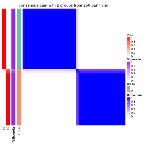
consensus_heatmap(res, k = 3)
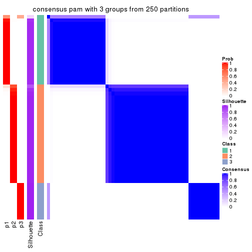
consensus_heatmap(res, k = 4)
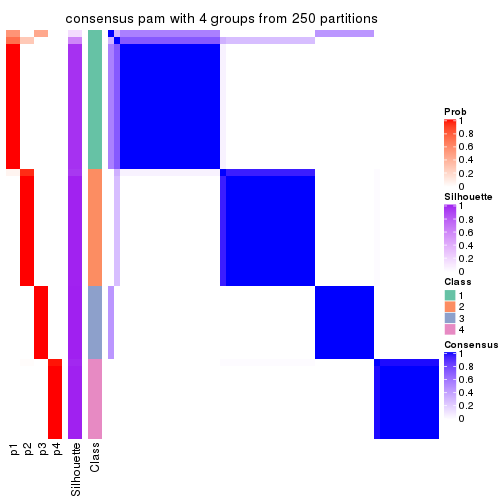
consensus_heatmap(res, k = 5)
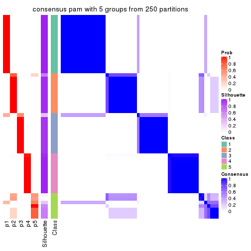
consensus_heatmap(res, k = 6)

Heatmaps for the membership of samples in all partitions to see how consistent they are:
membership_heatmap(res, k = 2)

membership_heatmap(res, k = 3)
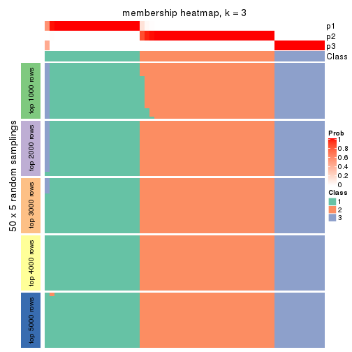
membership_heatmap(res, k = 4)
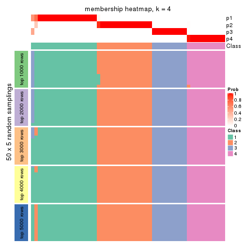
membership_heatmap(res, k = 5)
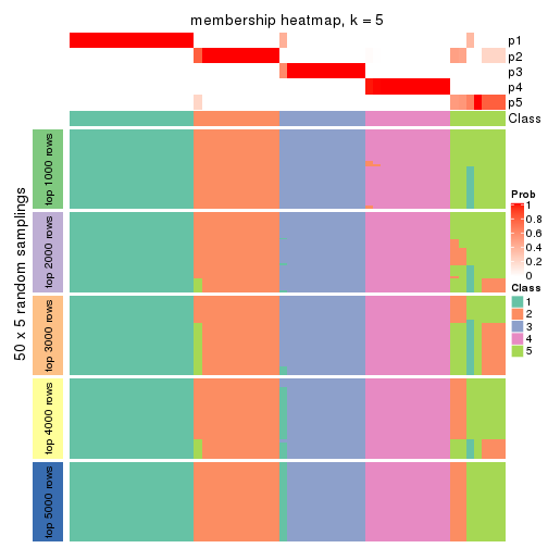
membership_heatmap(res, k = 6)
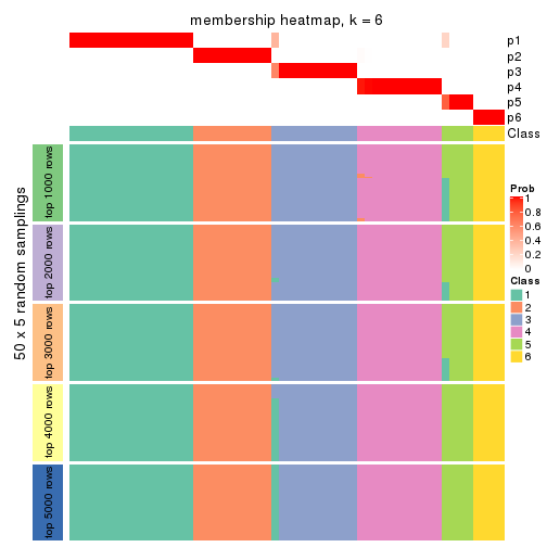
As soon as we have had the classes for columns, we can look for signatures which are significantly different between classes which can be candidate marks for certain classes. Following are the heatmaps for signatures.
Signature heatmaps where rows are scaled:
get_signatures(res, k = 2)
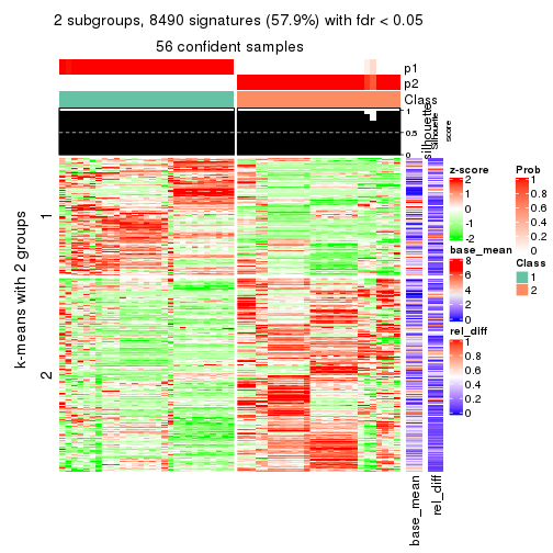
get_signatures(res, k = 3)
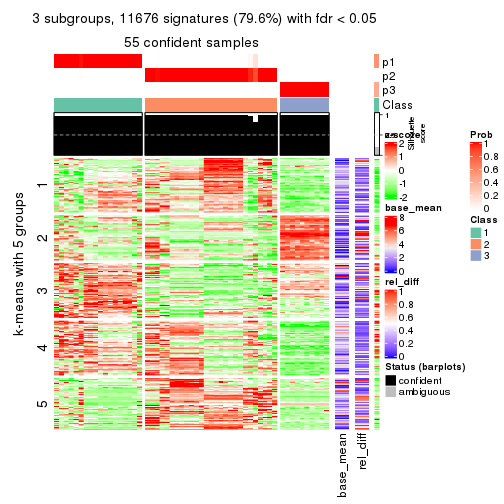
get_signatures(res, k = 4)
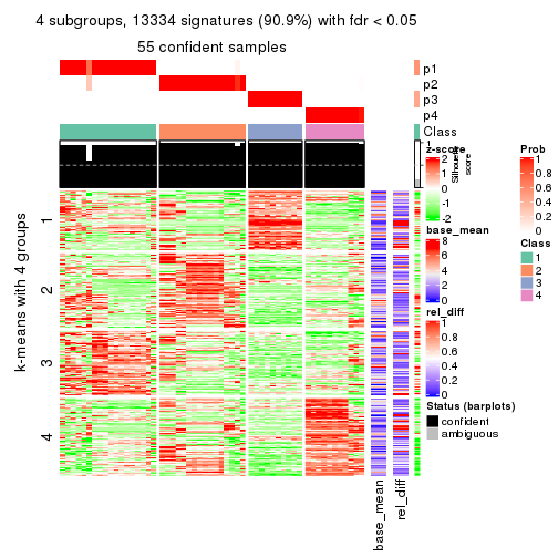
get_signatures(res, k = 5)
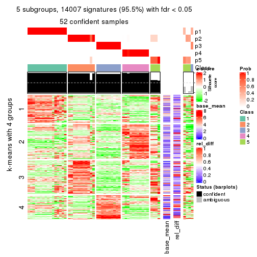
get_signatures(res, k = 6)
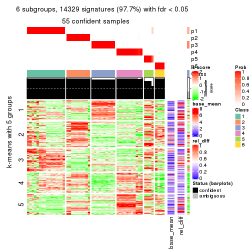
Signature heatmaps where rows are not scaled:
get_signatures(res, k = 2, scale_rows = FALSE)
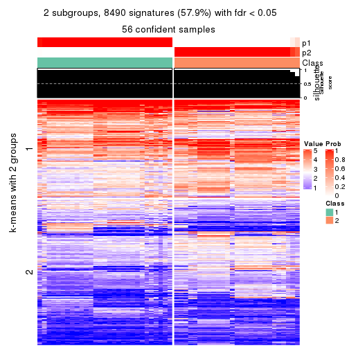
get_signatures(res, k = 3, scale_rows = FALSE)
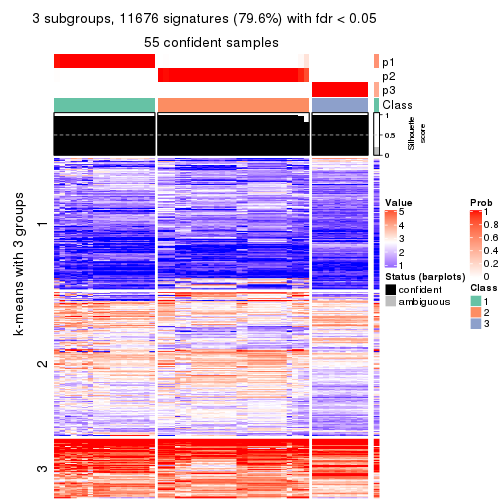
get_signatures(res, k = 4, scale_rows = FALSE)
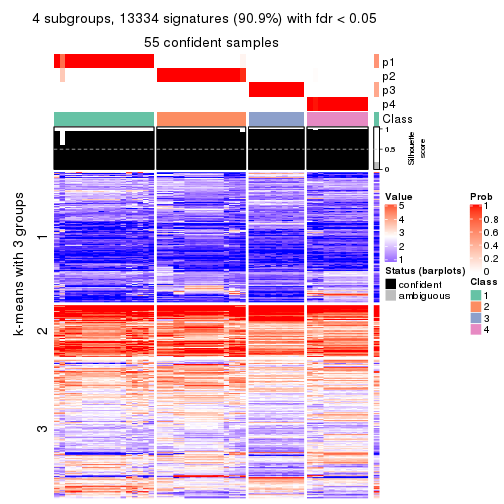
get_signatures(res, k = 5, scale_rows = FALSE)
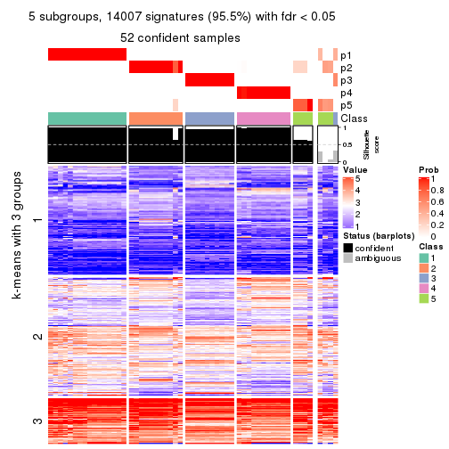
get_signatures(res, k = 6, scale_rows = FALSE)
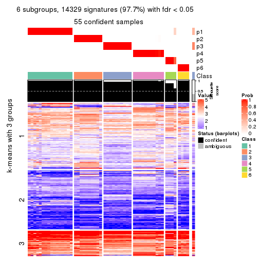
Compare the overlap of signatures from different k:
compare_signatures(res)
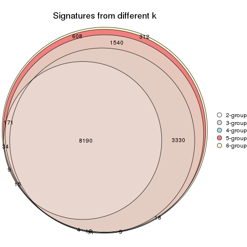
get_signature() returns a data frame invisibly. TO get the list of signatures, the function
call should be assigned to a variable explicitly. In following code, if plot argument is set
to FALSE, no heatmap is plotted while only the differential analysis is performed.
# code only for demonstration
tb = get_signature(res, k = ..., plot = FALSE)
An example of the output of tb is:
#> which_row fdr mean_1 mean_2 scaled_mean_1 scaled_mean_2 km
#> 1 38 0.042760348 8.373488 9.131774 -0.5533452 0.5164555 1
#> 2 40 0.018707592 7.106213 8.469186 -0.6173731 0.5762149 1
#> 3 55 0.019134737 10.221463 11.207825 -0.6159697 0.5749050 1
#> 4 59 0.006059896 5.921854 7.869574 -0.6899429 0.6439467 1
#> 5 60 0.018055526 8.928898 10.211722 -0.6204761 0.5791110 1
#> 6 98 0.009384629 15.714769 14.887706 0.6635654 -0.6193277 2
...
The columns in tb are:
which_row: row indices corresponding to the input matrix.fdr: FDR for the differential test. mean_x: The mean value in group x.scaled_mean_x: The mean value in group x after rows are scaled.km: Row groups if k-means clustering is applied to rows.UMAP plot which shows how samples are separated.
dimension_reduction(res, k = 2, method = "UMAP")

dimension_reduction(res, k = 3, method = "UMAP")
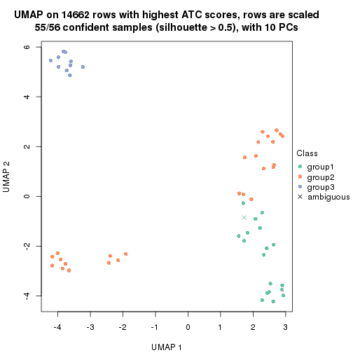
dimension_reduction(res, k = 4, method = "UMAP")
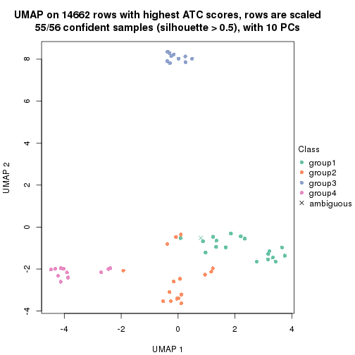
dimension_reduction(res, k = 5, method = "UMAP")
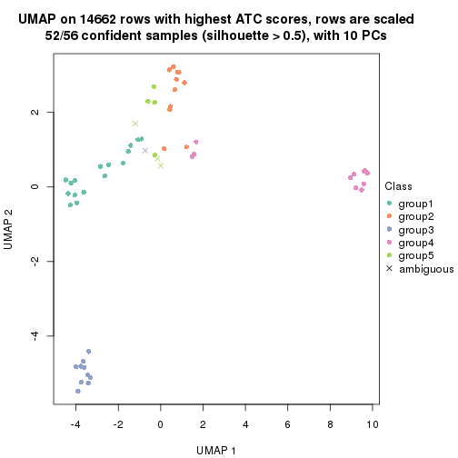
dimension_reduction(res, k = 6, method = "UMAP")

Following heatmap shows how subgroups are split when increasing k:
collect_classes(res)
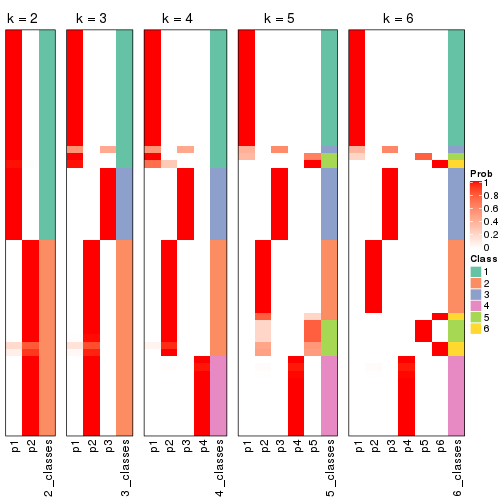
If matrix rows can be associated to genes, consider to use functional_enrichment(res,
...) to perform function enrichment for the signature genes. See this vignette for more detailed explanations.
The object with results only for a single top-value method and a single partition method can be extracted as:
res = res_list["ATC", "mclust"]
# you can also extract it by
# res = res_list["ATC:mclust"]
A summary of res and all the functions that can be applied to it:
res
#> A 'ConsensusPartition' object with k = 2, 3, 4, 5, 6.
#> On a matrix with 14662 rows and 56 columns.
#> Top rows (1000, 2000, 3000, 4000, 5000) are extracted by 'ATC' method.
#> Subgroups are detected by 'mclust' method.
#> Performed in total 1250 partitions by row resampling.
#> Best k for subgroups seems to be 6.
#>
#> Following methods can be applied to this 'ConsensusPartition' object:
#> [1] "cola_report" "collect_classes" "collect_plots"
#> [4] "collect_stats" "colnames" "compare_signatures"
#> [7] "consensus_heatmap" "dimension_reduction" "functional_enrichment"
#> [10] "get_anno_col" "get_anno" "get_classes"
#> [13] "get_consensus" "get_matrix" "get_membership"
#> [16] "get_param" "get_signatures" "get_stats"
#> [19] "is_best_k" "is_stable_k" "membership_heatmap"
#> [22] "ncol" "nrow" "plot_ecdf"
#> [25] "rownames" "select_partition_number" "show"
#> [28] "suggest_best_k" "test_to_known_factors"
collect_plots() function collects all the plots made from res for all k (number of partitions)
into one single page to provide an easy and fast comparison between different k.
collect_plots(res)
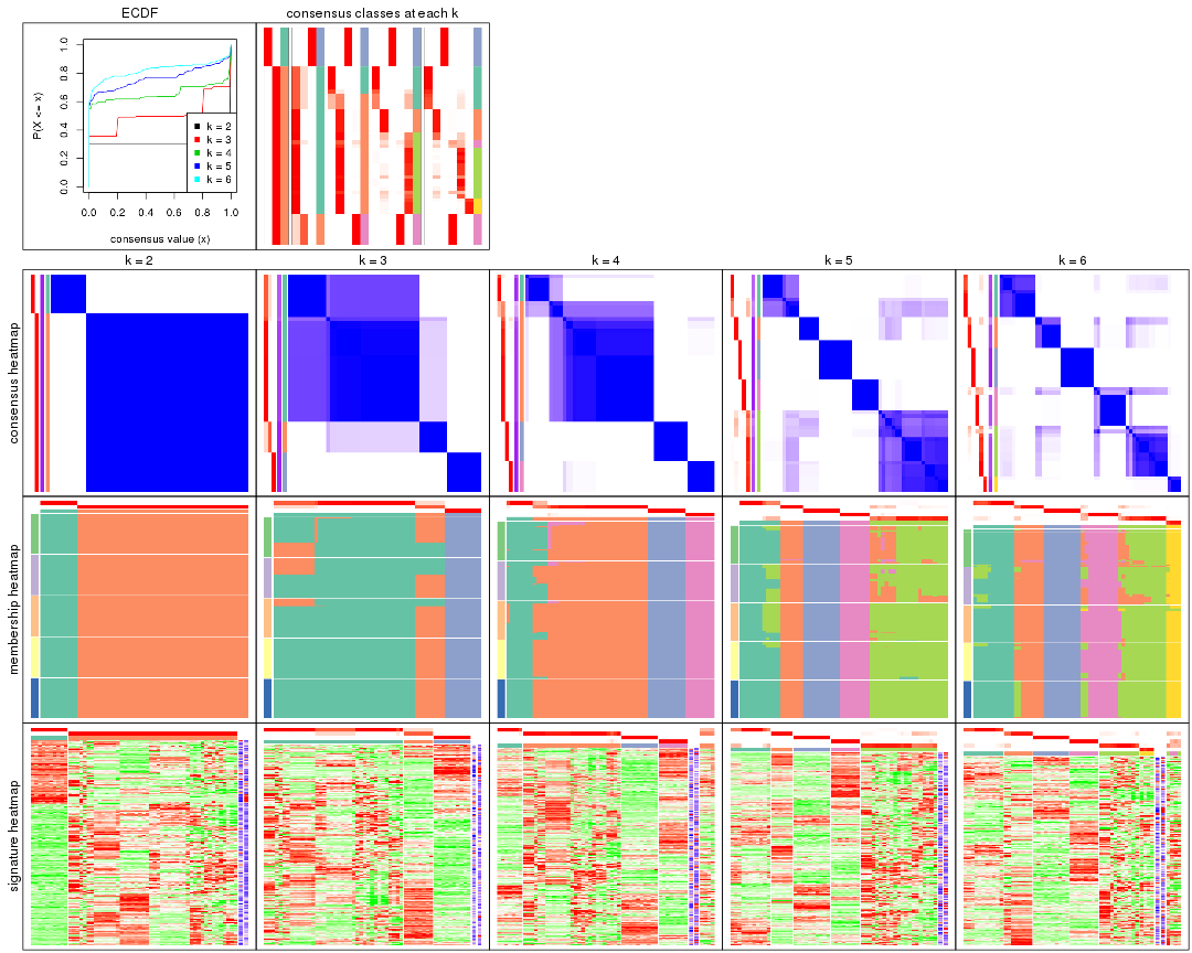
The plots are:
k and the heatmap of
predicted classes for each k.k.k.k.All the plots in panels can be made by individual functions and they are plotted later in this section.
select_partition_number() produces several plots showing different
statistics for choosing “optimized” k. There are following statistics:
k;k, the area increased is defined as \(A_k - A_{k-1}\).The detailed explanations of these statistics can be found in the cola vignette.
Generally speaking, lower PAC score, higher mean silhouette score or higher
concordance corresponds to better partition. Rand index and Jaccard index
measure how similar the current partition is compared to partition with k-1.
If they are too similar, we won't accept k is better than k-1.
select_partition_number(res)
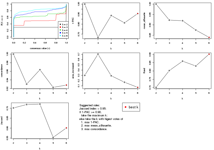
The numeric values for all these statistics can be obtained by get_stats().
get_stats(res)
#> k 1-PAC mean_silhouette concordance area_increased Rand Jaccard
#> 2 2 1.000 1.000 1.000 0.2994 0.701 0.701
#> 3 3 0.667 0.923 0.930 0.7028 0.803 0.719
#> 4 4 0.886 0.920 0.964 0.2915 0.859 0.720
#> 5 5 0.813 0.875 0.923 0.1688 0.830 0.554
#> 6 6 0.906 0.840 0.928 0.0714 0.901 0.601
suggest_best_k() suggests the best \(k\) based on these statistics. The rules are as follows:
suggest_best_k(res)
#> [1] 6
#> attr(,"optional")
#> [1] 2
There is also optional best \(k\) = 2 that is worth to check.
Following shows the table of the partitions (You need to click the show/hide
code output link to see it). The membership matrix (columns with name p*)
is inferred by
clue::cl_consensus()
function with the SE method. Basically the value in the membership matrix
represents the probability to belong to a certain group. The finall class
label for an item is determined with the group with highest probability it
belongs to.
In get_classes() function, the entropy is calculated from the membership
matrix and the silhouette score is calculated from the consensus matrix.
cbind(get_classes(res, k = 2), get_membership(res, k = 2))
#> class entropy silhouette p1 p2
#> SRR073723 2 0 1 0 1
#> SRR073724 2 0 1 0 1
#> SRR073725 2 0 1 0 1
#> SRR073726 2 0 1 0 1
#> SRR073727 2 0 1 0 1
#> SRR073728 2 0 1 0 1
#> SRR073729 2 0 1 0 1
#> SRR073730 2 0 1 0 1
#> SRR073731 2 0 1 0 1
#> SRR073732 2 0 1 0 1
#> SRR073733 2 0 1 0 1
#> SRR073734 2 0 1 0 1
#> SRR073735 2 0 1 0 1
#> SRR073736 2 0 1 0 1
#> SRR073737 2 0 1 0 1
#> SRR073738 2 0 1 0 1
#> SRR073739 2 0 1 0 1
#> SRR073740 2 0 1 0 1
#> SRR073741 2 0 1 0 1
#> SRR073742 2 0 1 0 1
#> SRR073743 2 0 1 0 1
#> SRR073744 2 0 1 0 1
#> SRR073745 2 0 1 0 1
#> SRR073746 2 0 1 0 1
#> SRR073747 2 0 1 0 1
#> SRR073748 2 0 1 0 1
#> SRR073749 2 0 1 0 1
#> SRR073750 2 0 1 0 1
#> SRR073751 2 0 1 0 1
#> SRR073752 2 0 1 0 1
#> SRR073753 2 0 1 0 1
#> SRR073754 2 0 1 0 1
#> SRR073755 2 0 1 0 1
#> SRR073756 2 0 1 0 1
#> SRR073758 2 0 1 0 1
#> SRR073759 2 0 1 0 1
#> SRR073760 2 0 1 0 1
#> SRR073761 2 0 1 0 1
#> SRR073763 2 0 1 0 1
#> SRR073764 2 0 1 0 1
#> SRR073765 2 0 1 0 1
#> SRR073766 2 0 1 0 1
#> SRR073767 2 0 1 0 1
#> SRR073768 2 0 1 0 1
#> SRR073769 1 0 1 1 0
#> SRR073770 1 0 1 1 0
#> SRR073771 1 0 1 1 0
#> SRR073772 1 0 1 1 0
#> SRR073773 1 0 1 1 0
#> SRR073774 1 0 1 1 0
#> SRR073775 1 0 1 1 0
#> SRR073776 1 0 1 1 0
#> SRR073777 1 0 1 1 0
#> SRR073778 1 0 1 1 0
#> SRR073779 2 0 1 0 1
#> SRR073780 2 0 1 0 1
cbind(get_classes(res, k = 3), get_membership(res, k = 3))
#> class entropy silhouette p1 p2 p3
#> SRR073723 1 0.0000 0.921 1.000 0.000 0
#> SRR073724 1 0.0000 0.921 1.000 0.000 0
#> SRR073725 1 0.0000 0.921 1.000 0.000 0
#> SRR073726 1 0.0000 0.921 1.000 0.000 0
#> SRR073727 1 0.0000 0.921 1.000 0.000 0
#> SRR073728 1 0.0000 0.921 1.000 0.000 0
#> SRR073729 1 0.0000 0.921 1.000 0.000 0
#> SRR073730 1 0.0000 0.921 1.000 0.000 0
#> SRR073731 1 0.0237 0.919 0.996 0.004 0
#> SRR073732 1 0.0237 0.919 0.996 0.004 0
#> SRR073733 1 0.0237 0.919 0.996 0.004 0
#> SRR073734 1 0.0237 0.919 0.996 0.004 0
#> SRR073735 1 0.0237 0.919 0.996 0.004 0
#> SRR073736 1 0.0237 0.919 0.996 0.004 0
#> SRR073737 1 0.0237 0.919 0.996 0.004 0
#> SRR073738 1 0.0000 0.921 1.000 0.000 0
#> SRR073739 1 0.4504 0.817 0.804 0.196 0
#> SRR073740 1 0.4504 0.817 0.804 0.196 0
#> SRR073741 1 0.4504 0.817 0.804 0.196 0
#> SRR073742 1 0.4504 0.817 0.804 0.196 0
#> SRR073743 1 0.4504 0.817 0.804 0.196 0
#> SRR073744 1 0.4504 0.817 0.804 0.196 0
#> SRR073745 1 0.4504 0.817 0.804 0.196 0
#> SRR073746 1 0.4504 0.817 0.804 0.196 0
#> SRR073747 1 0.4504 0.817 0.804 0.196 0
#> SRR073748 1 0.4504 0.817 0.804 0.196 0
#> SRR073749 1 0.4504 0.817 0.804 0.196 0
#> SRR073750 1 0.0000 0.921 1.000 0.000 0
#> SRR073751 1 0.0000 0.921 1.000 0.000 0
#> SRR073752 1 0.0000 0.921 1.000 0.000 0
#> SRR073753 1 0.0000 0.921 1.000 0.000 0
#> SRR073754 1 0.0000 0.921 1.000 0.000 0
#> SRR073755 1 0.3551 0.767 0.868 0.132 0
#> SRR073756 1 0.0424 0.917 0.992 0.008 0
#> SRR073758 1 0.0424 0.917 0.992 0.008 0
#> SRR073759 1 0.0000 0.921 1.000 0.000 0
#> SRR073760 2 0.4504 1.000 0.196 0.804 0
#> SRR073761 2 0.4504 1.000 0.196 0.804 0
#> SRR073763 2 0.4504 1.000 0.196 0.804 0
#> SRR073764 2 0.4504 1.000 0.196 0.804 0
#> SRR073765 2 0.4504 1.000 0.196 0.804 0
#> SRR073766 2 0.4504 1.000 0.196 0.804 0
#> SRR073767 2 0.4504 1.000 0.196 0.804 0
#> SRR073768 2 0.4504 1.000 0.196 0.804 0
#> SRR073769 3 0.0000 1.000 0.000 0.000 1
#> SRR073770 3 0.0000 1.000 0.000 0.000 1
#> SRR073771 3 0.0000 1.000 0.000 0.000 1
#> SRR073772 3 0.0000 1.000 0.000 0.000 1
#> SRR073773 3 0.0000 1.000 0.000 0.000 1
#> SRR073774 3 0.0000 1.000 0.000 0.000 1
#> SRR073775 3 0.0000 1.000 0.000 0.000 1
#> SRR073776 3 0.0000 1.000 0.000 0.000 1
#> SRR073777 3 0.0000 1.000 0.000 0.000 1
#> SRR073778 3 0.0000 1.000 0.000 0.000 1
#> SRR073779 1 0.0000 0.921 1.000 0.000 0
#> SRR073780 1 0.0000 0.921 1.000 0.000 0
cbind(get_classes(res, k = 4), get_membership(res, k = 4))
#> class entropy silhouette p1 p2 p3 p4
#> SRR073723 2 0.0000 0.934 0.000 1.000 0 0.000
#> SRR073724 2 0.0000 0.934 0.000 1.000 0 0.000
#> SRR073725 2 0.0000 0.934 0.000 1.000 0 0.000
#> SRR073726 2 0.0000 0.934 0.000 1.000 0 0.000
#> SRR073727 2 0.0000 0.934 0.000 1.000 0 0.000
#> SRR073728 2 0.0000 0.934 0.000 1.000 0 0.000
#> SRR073729 2 0.0000 0.934 0.000 1.000 0 0.000
#> SRR073730 2 0.0000 0.934 0.000 1.000 0 0.000
#> SRR073731 2 0.0707 0.928 0.000 0.980 0 0.020
#> SRR073732 2 0.0592 0.930 0.000 0.984 0 0.016
#> SRR073733 2 0.0707 0.928 0.000 0.980 0 0.020
#> SRR073734 2 0.0707 0.928 0.000 0.980 0 0.020
#> SRR073735 2 0.0707 0.928 0.000 0.980 0 0.020
#> SRR073736 2 0.0707 0.928 0.000 0.980 0 0.020
#> SRR073737 2 0.0707 0.928 0.000 0.980 0 0.020
#> SRR073738 2 0.0000 0.934 0.000 1.000 0 0.000
#> SRR073739 1 0.0000 0.970 1.000 0.000 0 0.000
#> SRR073740 1 0.0000 0.970 1.000 0.000 0 0.000
#> SRR073741 1 0.0000 0.970 1.000 0.000 0 0.000
#> SRR073742 1 0.0000 0.970 1.000 0.000 0 0.000
#> SRR073743 1 0.0000 0.970 1.000 0.000 0 0.000
#> SRR073744 1 0.0000 0.970 1.000 0.000 0 0.000
#> SRR073745 1 0.2589 0.815 0.884 0.116 0 0.000
#> SRR073746 2 0.4830 0.426 0.392 0.608 0 0.000
#> SRR073747 2 0.4713 0.497 0.360 0.640 0 0.000
#> SRR073748 2 0.4713 0.497 0.360 0.640 0 0.000
#> SRR073749 2 0.4713 0.497 0.360 0.640 0 0.000
#> SRR073750 2 0.0000 0.934 0.000 1.000 0 0.000
#> SRR073751 2 0.0000 0.934 0.000 1.000 0 0.000
#> SRR073752 2 0.0000 0.934 0.000 1.000 0 0.000
#> SRR073753 2 0.0000 0.934 0.000 1.000 0 0.000
#> SRR073754 2 0.0000 0.934 0.000 1.000 0 0.000
#> SRR073755 2 0.3400 0.790 0.000 0.820 0 0.180
#> SRR073756 2 0.1637 0.903 0.000 0.940 0 0.060
#> SRR073758 2 0.1637 0.903 0.000 0.940 0 0.060
#> SRR073759 2 0.0000 0.934 0.000 1.000 0 0.000
#> SRR073760 4 0.0000 1.000 0.000 0.000 0 1.000
#> SRR073761 4 0.0000 1.000 0.000 0.000 0 1.000
#> SRR073763 4 0.0000 1.000 0.000 0.000 0 1.000
#> SRR073764 4 0.0000 1.000 0.000 0.000 0 1.000
#> SRR073765 4 0.0000 1.000 0.000 0.000 0 1.000
#> SRR073766 4 0.0000 1.000 0.000 0.000 0 1.000
#> SRR073767 4 0.0000 1.000 0.000 0.000 0 1.000
#> SRR073768 4 0.0000 1.000 0.000 0.000 0 1.000
#> SRR073769 3 0.0000 1.000 0.000 0.000 1 0.000
#> SRR073770 3 0.0000 1.000 0.000 0.000 1 0.000
#> SRR073771 3 0.0000 1.000 0.000 0.000 1 0.000
#> SRR073772 3 0.0000 1.000 0.000 0.000 1 0.000
#> SRR073773 3 0.0000 1.000 0.000 0.000 1 0.000
#> SRR073774 3 0.0000 1.000 0.000 0.000 1 0.000
#> SRR073775 3 0.0000 1.000 0.000 0.000 1 0.000
#> SRR073776 3 0.0000 1.000 0.000 0.000 1 0.000
#> SRR073777 3 0.0000 1.000 0.000 0.000 1 0.000
#> SRR073778 3 0.0000 1.000 0.000 0.000 1 0.000
#> SRR073779 2 0.0000 0.934 0.000 1.000 0 0.000
#> SRR073780 2 0.0000 0.934 0.000 1.000 0 0.000
cbind(get_classes(res, k = 5), get_membership(res, k = 5))
#> class entropy silhouette p1 p2 p3 p4 p5
#> SRR073723 5 0.0579 0.858 0.008 0.008 0 0.000 0.984
#> SRR073724 5 0.0703 0.848 0.024 0.000 0 0.000 0.976
#> SRR073725 5 0.0703 0.848 0.024 0.000 0 0.000 0.976
#> SRR073726 5 0.1908 0.858 0.000 0.092 0 0.000 0.908
#> SRR073727 5 0.0703 0.848 0.024 0.000 0 0.000 0.976
#> SRR073728 5 0.1341 0.871 0.000 0.056 0 0.000 0.944
#> SRR073729 5 0.1341 0.871 0.000 0.056 0 0.000 0.944
#> SRR073730 5 0.1341 0.871 0.000 0.056 0 0.000 0.944
#> SRR073731 2 0.0162 1.000 0.000 0.996 0 0.004 0.000
#> SRR073732 5 0.4152 0.714 0.000 0.296 0 0.012 0.692
#> SRR073733 2 0.0162 1.000 0.000 0.996 0 0.004 0.000
#> SRR073734 2 0.0162 1.000 0.000 0.996 0 0.004 0.000
#> SRR073735 2 0.0162 1.000 0.000 0.996 0 0.004 0.000
#> SRR073736 2 0.0162 1.000 0.000 0.996 0 0.004 0.000
#> SRR073737 2 0.0162 1.000 0.000 0.996 0 0.004 0.000
#> SRR073738 5 0.0703 0.848 0.024 0.000 0 0.000 0.976
#> SRR073739 1 0.0000 0.778 1.000 0.000 0 0.000 0.000
#> SRR073740 1 0.0000 0.778 1.000 0.000 0 0.000 0.000
#> SRR073741 1 0.0000 0.778 1.000 0.000 0 0.000 0.000
#> SRR073742 1 0.0000 0.778 1.000 0.000 0 0.000 0.000
#> SRR073743 1 0.0000 0.778 1.000 0.000 0 0.000 0.000
#> SRR073744 1 0.0000 0.778 1.000 0.000 0 0.000 0.000
#> SRR073745 1 0.3074 0.738 0.804 0.000 0 0.000 0.196
#> SRR073746 1 0.4126 0.610 0.620 0.000 0 0.000 0.380
#> SRR073747 1 0.4074 0.638 0.636 0.000 0 0.000 0.364
#> SRR073748 1 0.4074 0.638 0.636 0.000 0 0.000 0.364
#> SRR073749 1 0.4074 0.638 0.636 0.000 0 0.000 0.364
#> SRR073750 5 0.0703 0.848 0.024 0.000 0 0.000 0.976
#> SRR073751 5 0.0963 0.870 0.000 0.036 0 0.000 0.964
#> SRR073752 5 0.4045 0.646 0.000 0.356 0 0.000 0.644
#> SRR073753 5 0.4030 0.652 0.000 0.352 0 0.000 0.648
#> SRR073754 5 0.0963 0.870 0.000 0.036 0 0.000 0.964
#> SRR073755 5 0.5067 0.731 0.000 0.172 0 0.128 0.700
#> SRR073756 5 0.4479 0.730 0.000 0.264 0 0.036 0.700
#> SRR073758 5 0.4479 0.730 0.000 0.264 0 0.036 0.700
#> SRR073759 5 0.2891 0.821 0.000 0.176 0 0.000 0.824
#> SRR073760 4 0.0000 1.000 0.000 0.000 0 1.000 0.000
#> SRR073761 4 0.0000 1.000 0.000 0.000 0 1.000 0.000
#> SRR073763 4 0.0000 1.000 0.000 0.000 0 1.000 0.000
#> SRR073764 4 0.0000 1.000 0.000 0.000 0 1.000 0.000
#> SRR073765 4 0.0000 1.000 0.000 0.000 0 1.000 0.000
#> SRR073766 4 0.0000 1.000 0.000 0.000 0 1.000 0.000
#> SRR073767 4 0.0000 1.000 0.000 0.000 0 1.000 0.000
#> SRR073768 4 0.0000 1.000 0.000 0.000 0 1.000 0.000
#> SRR073769 3 0.0000 1.000 0.000 0.000 1 0.000 0.000
#> SRR073770 3 0.0000 1.000 0.000 0.000 1 0.000 0.000
#> SRR073771 3 0.0000 1.000 0.000 0.000 1 0.000 0.000
#> SRR073772 3 0.0000 1.000 0.000 0.000 1 0.000 0.000
#> SRR073773 3 0.0000 1.000 0.000 0.000 1 0.000 0.000
#> SRR073774 3 0.0000 1.000 0.000 0.000 1 0.000 0.000
#> SRR073775 3 0.0000 1.000 0.000 0.000 1 0.000 0.000
#> SRR073776 3 0.0000 1.000 0.000 0.000 1 0.000 0.000
#> SRR073777 3 0.0000 1.000 0.000 0.000 1 0.000 0.000
#> SRR073778 3 0.0000 1.000 0.000 0.000 1 0.000 0.000
#> SRR073779 5 0.0963 0.870 0.000 0.036 0 0.000 0.964
#> SRR073780 5 0.0963 0.870 0.000 0.036 0 0.000 0.964
cbind(get_classes(res, k = 6), get_membership(res, k = 6))
#> class entropy silhouette p1 p2 p3 p4 p5 p6
#> SRR073723 5 0.0790 0.8686 0.000 0.032 0 0.000 0.968 0.000
#> SRR073724 5 0.0000 0.8612 0.000 0.000 0 0.000 1.000 0.000
#> SRR073725 5 0.0790 0.8682 0.000 0.032 0 0.000 0.968 0.000
#> SRR073726 6 0.1807 0.9140 0.000 0.020 0 0.000 0.060 0.920
#> SRR073727 5 0.0000 0.8612 0.000 0.000 0 0.000 1.000 0.000
#> SRR073728 5 0.1501 0.8624 0.000 0.076 0 0.000 0.924 0.000
#> SRR073729 5 0.1501 0.8624 0.000 0.076 0 0.000 0.924 0.000
#> SRR073730 5 0.1501 0.8624 0.000 0.076 0 0.000 0.924 0.000
#> SRR073731 2 0.0508 0.8953 0.000 0.984 0 0.012 0.004 0.000
#> SRR073732 5 0.4570 0.3797 0.000 0.364 0 0.020 0.600 0.016
#> SRR073733 2 0.0508 0.8953 0.000 0.984 0 0.012 0.004 0.000
#> SRR073734 2 0.0508 0.8953 0.000 0.984 0 0.012 0.004 0.000
#> SRR073735 2 0.0508 0.8953 0.000 0.984 0 0.012 0.004 0.000
#> SRR073736 2 0.0508 0.8953 0.000 0.984 0 0.012 0.004 0.000
#> SRR073737 2 0.0508 0.8953 0.000 0.984 0 0.012 0.004 0.000
#> SRR073738 5 0.0000 0.8612 0.000 0.000 0 0.000 1.000 0.000
#> SRR073739 1 0.0000 0.9282 1.000 0.000 0 0.000 0.000 0.000
#> SRR073740 1 0.0000 0.9282 1.000 0.000 0 0.000 0.000 0.000
#> SRR073741 1 0.0000 0.9282 1.000 0.000 0 0.000 0.000 0.000
#> SRR073742 1 0.0000 0.9282 1.000 0.000 0 0.000 0.000 0.000
#> SRR073743 1 0.0000 0.9282 1.000 0.000 0 0.000 0.000 0.000
#> SRR073744 1 0.0000 0.9282 1.000 0.000 0 0.000 0.000 0.000
#> SRR073745 1 0.1075 0.9186 0.952 0.000 0 0.000 0.048 0.000
#> SRR073746 1 0.1910 0.8942 0.892 0.000 0 0.000 0.108 0.000
#> SRR073747 1 0.2442 0.8785 0.852 0.004 0 0.000 0.144 0.000
#> SRR073748 1 0.2442 0.8785 0.852 0.004 0 0.000 0.144 0.000
#> SRR073749 1 0.2442 0.8785 0.852 0.004 0 0.000 0.144 0.000
#> SRR073750 5 0.0000 0.8612 0.000 0.000 0 0.000 1.000 0.000
#> SRR073751 5 0.1204 0.8670 0.000 0.056 0 0.000 0.944 0.000
#> SRR073752 2 0.3175 0.6186 0.000 0.744 0 0.000 0.256 0.000
#> SRR073753 2 0.3175 0.6186 0.000 0.744 0 0.000 0.256 0.000
#> SRR073754 6 0.0458 0.9724 0.000 0.000 0 0.000 0.016 0.984
#> SRR073755 4 0.5962 0.1311 0.000 0.152 0 0.492 0.340 0.016
#> SRR073756 5 0.6428 -0.0161 0.000 0.260 0 0.352 0.372 0.016
#> SRR073758 4 0.6428 -0.0972 0.000 0.260 0 0.372 0.352 0.016
#> SRR073759 5 0.2491 0.7819 0.000 0.164 0 0.000 0.836 0.000
#> SRR073760 4 0.0000 0.8445 0.000 0.000 0 1.000 0.000 0.000
#> SRR073761 4 0.0000 0.8445 0.000 0.000 0 1.000 0.000 0.000
#> SRR073763 4 0.0000 0.8445 0.000 0.000 0 1.000 0.000 0.000
#> SRR073764 4 0.0000 0.8445 0.000 0.000 0 1.000 0.000 0.000
#> SRR073765 4 0.0000 0.8445 0.000 0.000 0 1.000 0.000 0.000
#> SRR073766 4 0.0000 0.8445 0.000 0.000 0 1.000 0.000 0.000
#> SRR073767 4 0.0000 0.8445 0.000 0.000 0 1.000 0.000 0.000
#> SRR073768 4 0.0000 0.8445 0.000 0.000 0 1.000 0.000 0.000
#> SRR073769 3 0.0000 1.0000 0.000 0.000 1 0.000 0.000 0.000
#> SRR073770 3 0.0000 1.0000 0.000 0.000 1 0.000 0.000 0.000
#> SRR073771 3 0.0000 1.0000 0.000 0.000 1 0.000 0.000 0.000
#> SRR073772 3 0.0000 1.0000 0.000 0.000 1 0.000 0.000 0.000
#> SRR073773 3 0.0000 1.0000 0.000 0.000 1 0.000 0.000 0.000
#> SRR073774 3 0.0000 1.0000 0.000 0.000 1 0.000 0.000 0.000
#> SRR073775 3 0.0000 1.0000 0.000 0.000 1 0.000 0.000 0.000
#> SRR073776 3 0.0000 1.0000 0.000 0.000 1 0.000 0.000 0.000
#> SRR073777 3 0.0000 1.0000 0.000 0.000 1 0.000 0.000 0.000
#> SRR073778 3 0.0000 1.0000 0.000 0.000 1 0.000 0.000 0.000
#> SRR073779 6 0.0458 0.9724 0.000 0.000 0 0.000 0.016 0.984
#> SRR073780 6 0.0458 0.9724 0.000 0.000 0 0.000 0.016 0.984
Heatmaps for the consensus matrix. It visualizes the probability of two samples to be in a same group.
consensus_heatmap(res, k = 2)
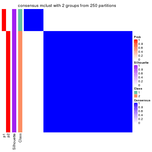
consensus_heatmap(res, k = 3)
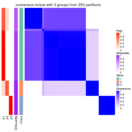
consensus_heatmap(res, k = 4)
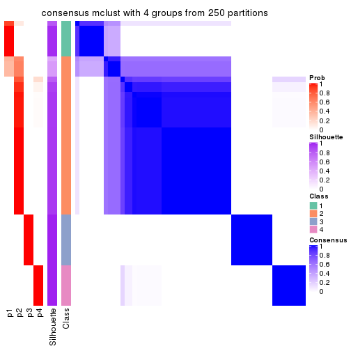
consensus_heatmap(res, k = 5)
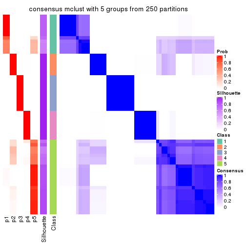
consensus_heatmap(res, k = 6)
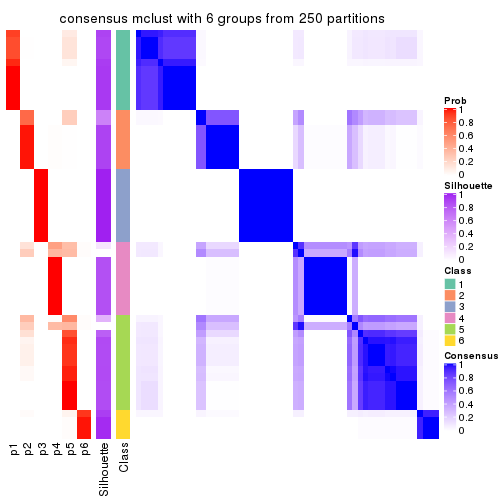
Heatmaps for the membership of samples in all partitions to see how consistent they are:
membership_heatmap(res, k = 2)

membership_heatmap(res, k = 3)
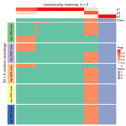
membership_heatmap(res, k = 4)
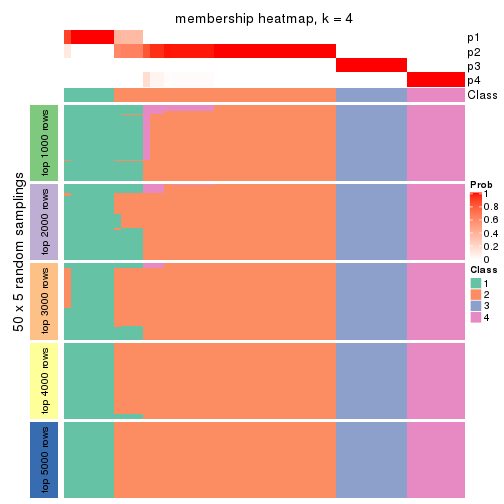
membership_heatmap(res, k = 5)
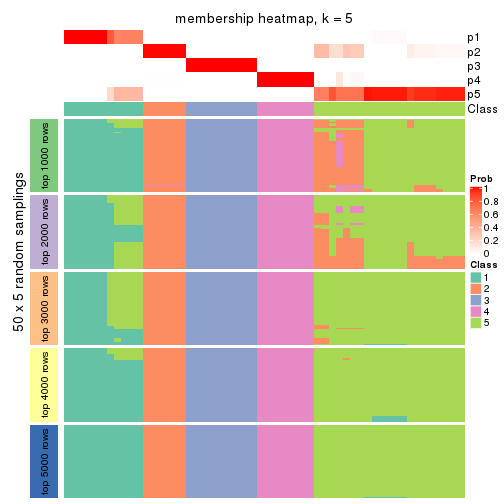
membership_heatmap(res, k = 6)
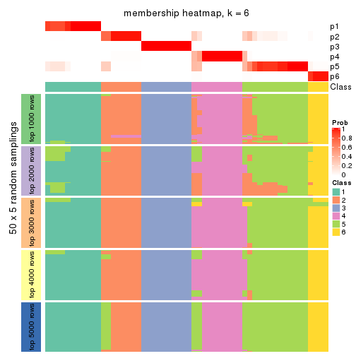
As soon as we have had the classes for columns, we can look for signatures which are significantly different between classes which can be candidate marks for certain classes. Following are the heatmaps for signatures.
Signature heatmaps where rows are scaled:
get_signatures(res, k = 2)

get_signatures(res, k = 3)
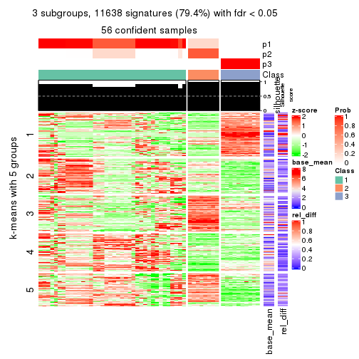
get_signatures(res, k = 4)
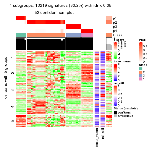
get_signatures(res, k = 5)
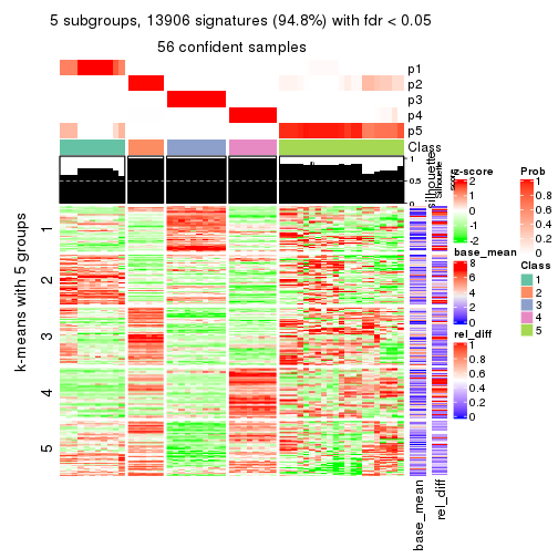
get_signatures(res, k = 6)
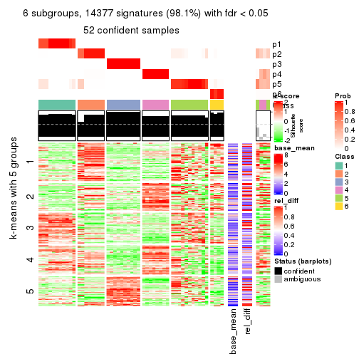
Signature heatmaps where rows are not scaled:
get_signatures(res, k = 2, scale_rows = FALSE)
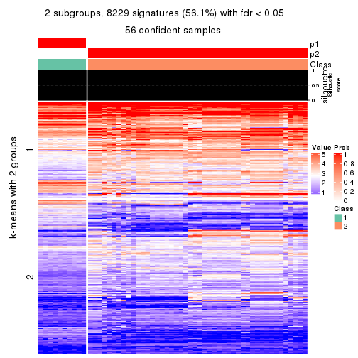
get_signatures(res, k = 3, scale_rows = FALSE)
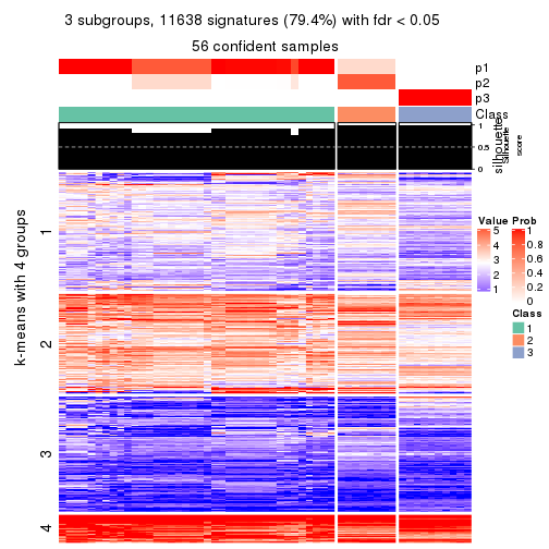
get_signatures(res, k = 4, scale_rows = FALSE)
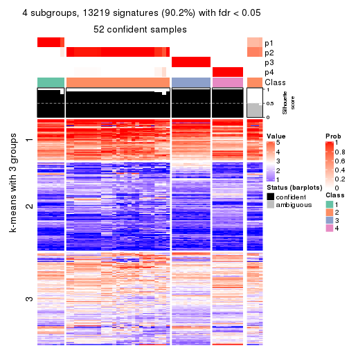
get_signatures(res, k = 5, scale_rows = FALSE)
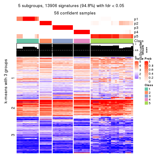
get_signatures(res, k = 6, scale_rows = FALSE)
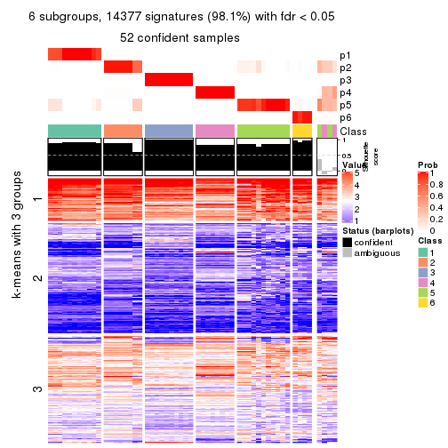
Compare the overlap of signatures from different k:
compare_signatures(res)
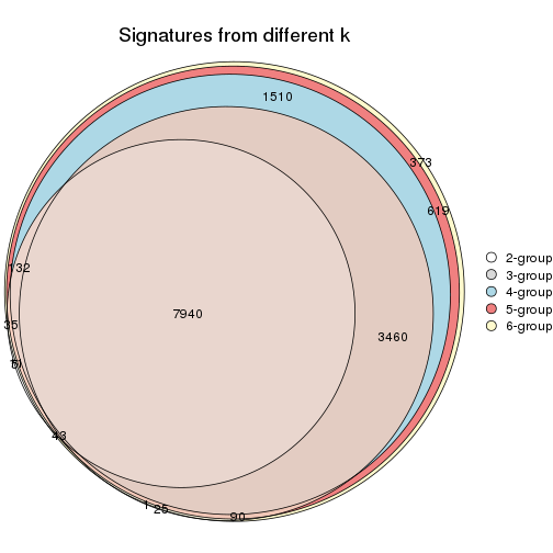
get_signature() returns a data frame invisibly. TO get the list of signatures, the function
call should be assigned to a variable explicitly. In following code, if plot argument is set
to FALSE, no heatmap is plotted while only the differential analysis is performed.
# code only for demonstration
tb = get_signature(res, k = ..., plot = FALSE)
An example of the output of tb is:
#> which_row fdr mean_1 mean_2 scaled_mean_1 scaled_mean_2 km
#> 1 38 0.042760348 8.373488 9.131774 -0.5533452 0.5164555 1
#> 2 40 0.018707592 7.106213 8.469186 -0.6173731 0.5762149 1
#> 3 55 0.019134737 10.221463 11.207825 -0.6159697 0.5749050 1
#> 4 59 0.006059896 5.921854 7.869574 -0.6899429 0.6439467 1
#> 5 60 0.018055526 8.928898 10.211722 -0.6204761 0.5791110 1
#> 6 98 0.009384629 15.714769 14.887706 0.6635654 -0.6193277 2
...
The columns in tb are:
which_row: row indices corresponding to the input matrix.fdr: FDR for the differential test. mean_x: The mean value in group x.scaled_mean_x: The mean value in group x after rows are scaled.km: Row groups if k-means clustering is applied to rows.UMAP plot which shows how samples are separated.
dimension_reduction(res, k = 2, method = "UMAP")

dimension_reduction(res, k = 3, method = "UMAP")
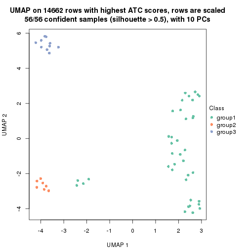
dimension_reduction(res, k = 4, method = "UMAP")
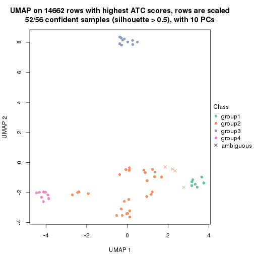
dimension_reduction(res, k = 5, method = "UMAP")
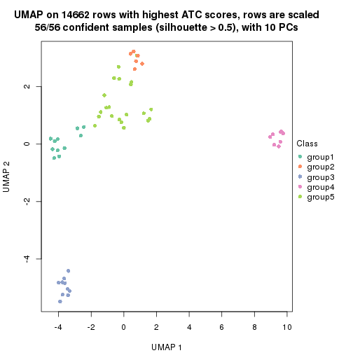
dimension_reduction(res, k = 6, method = "UMAP")

Following heatmap shows how subgroups are split when increasing k:
collect_classes(res)
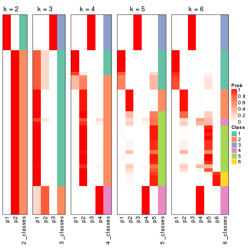
If matrix rows can be associated to genes, consider to use functional_enrichment(res,
...) to perform function enrichment for the signature genes. See this vignette for more detailed explanations.
The object with results only for a single top-value method and a single partition method can be extracted as:
res = res_list["ATC", "NMF"]
# you can also extract it by
# res = res_list["ATC:NMF"]
A summary of res and all the functions that can be applied to it:
res
#> A 'ConsensusPartition' object with k = 2, 3, 4, 5, 6.
#> On a matrix with 14662 rows and 56 columns.
#> Top rows (1000, 2000, 3000, 4000, 5000) are extracted by 'ATC' method.
#> Subgroups are detected by 'NMF' method.
#> Performed in total 1250 partitions by row resampling.
#> Best k for subgroups seems to be 2.
#>
#> Following methods can be applied to this 'ConsensusPartition' object:
#> [1] "cola_report" "collect_classes" "collect_plots"
#> [4] "collect_stats" "colnames" "compare_signatures"
#> [7] "consensus_heatmap" "dimension_reduction" "functional_enrichment"
#> [10] "get_anno_col" "get_anno" "get_classes"
#> [13] "get_consensus" "get_matrix" "get_membership"
#> [16] "get_param" "get_signatures" "get_stats"
#> [19] "is_best_k" "is_stable_k" "membership_heatmap"
#> [22] "ncol" "nrow" "plot_ecdf"
#> [25] "rownames" "select_partition_number" "show"
#> [28] "suggest_best_k" "test_to_known_factors"
collect_plots() function collects all the plots made from res for all k (number of partitions)
into one single page to provide an easy and fast comparison between different k.
collect_plots(res)
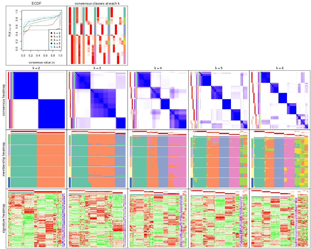
The plots are:
k and the heatmap of
predicted classes for each k.k.k.k.All the plots in panels can be made by individual functions and they are plotted later in this section.
select_partition_number() produces several plots showing different
statistics for choosing “optimized” k. There are following statistics:
k;k, the area increased is defined as \(A_k - A_{k-1}\).The detailed explanations of these statistics can be found in the cola vignette.
Generally speaking, lower PAC score, higher mean silhouette score or higher
concordance corresponds to better partition. Rand index and Jaccard index
measure how similar the current partition is compared to partition with k-1.
If they are too similar, we won't accept k is better than k-1.
select_partition_number(res)
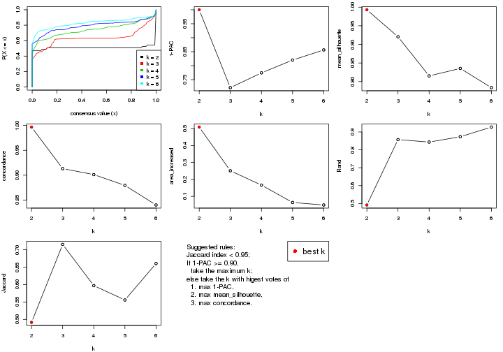
The numeric values for all these statistics can be obtained by get_stats().
get_stats(res)
#> k 1-PAC mean_silhouette concordance area_increased Rand Jaccard
#> 2 2 1.000 0.993 0.997 0.5088 0.492 0.492
#> 3 3 0.721 0.920 0.913 0.2511 0.857 0.715
#> 4 4 0.774 0.815 0.901 0.1663 0.844 0.597
#> 5 5 0.820 0.835 0.879 0.0638 0.873 0.556
#> 6 6 0.856 0.784 0.840 0.0491 0.927 0.661
suggest_best_k() suggests the best \(k\) based on these statistics. The rules are as follows:
suggest_best_k(res)
#> [1] 2
Following shows the table of the partitions (You need to click the show/hide
code output link to see it). The membership matrix (columns with name p*)
is inferred by
clue::cl_consensus()
function with the SE method. Basically the value in the membership matrix
represents the probability to belong to a certain group. The finall class
label for an item is determined with the group with highest probability it
belongs to.
In get_classes() function, the entropy is calculated from the membership
matrix and the silhouette score is calculated from the consensus matrix.
cbind(get_classes(res, k = 2), get_membership(res, k = 2))
#> class entropy silhouette p1 p2
#> SRR073723 1 0.000 0.996 1.000 0.000
#> SRR073724 1 0.000 0.996 1.000 0.000
#> SRR073725 1 0.000 0.996 1.000 0.000
#> SRR073726 2 0.000 0.997 0.000 1.000
#> SRR073727 1 0.000 0.996 1.000 0.000
#> SRR073728 2 0.000 0.997 0.000 1.000
#> SRR073729 2 0.000 0.997 0.000 1.000
#> SRR073730 2 0.000 0.997 0.000 1.000
#> SRR073731 2 0.000 0.997 0.000 1.000
#> SRR073732 2 0.000 0.997 0.000 1.000
#> SRR073733 2 0.000 0.997 0.000 1.000
#> SRR073734 2 0.000 0.997 0.000 1.000
#> SRR073735 2 0.000 0.997 0.000 1.000
#> SRR073736 2 0.000 0.997 0.000 1.000
#> SRR073737 2 0.000 0.997 0.000 1.000
#> SRR073738 1 0.000 0.996 1.000 0.000
#> SRR073739 1 0.000 0.996 1.000 0.000
#> SRR073740 1 0.000 0.996 1.000 0.000
#> SRR073741 1 0.000 0.996 1.000 0.000
#> SRR073742 1 0.000 0.996 1.000 0.000
#> SRR073743 1 0.000 0.996 1.000 0.000
#> SRR073744 1 0.000 0.996 1.000 0.000
#> SRR073745 1 0.000 0.996 1.000 0.000
#> SRR073746 2 0.373 0.922 0.072 0.928
#> SRR073747 1 0.000 0.996 1.000 0.000
#> SRR073748 1 0.000 0.996 1.000 0.000
#> SRR073749 1 0.000 0.996 1.000 0.000
#> SRR073750 1 0.000 0.996 1.000 0.000
#> SRR073751 1 0.506 0.873 0.888 0.112
#> SRR073752 2 0.000 0.997 0.000 1.000
#> SRR073753 2 0.000 0.997 0.000 1.000
#> SRR073754 2 0.000 0.997 0.000 1.000
#> SRR073755 2 0.000 0.997 0.000 1.000
#> SRR073756 2 0.000 0.997 0.000 1.000
#> SRR073758 2 0.000 0.997 0.000 1.000
#> SRR073759 2 0.000 0.997 0.000 1.000
#> SRR073760 2 0.000 0.997 0.000 1.000
#> SRR073761 2 0.000 0.997 0.000 1.000
#> SRR073763 2 0.000 0.997 0.000 1.000
#> SRR073764 2 0.000 0.997 0.000 1.000
#> SRR073765 2 0.000 0.997 0.000 1.000
#> SRR073766 2 0.000 0.997 0.000 1.000
#> SRR073767 2 0.000 0.997 0.000 1.000
#> SRR073768 2 0.000 0.997 0.000 1.000
#> SRR073769 1 0.000 0.996 1.000 0.000
#> SRR073770 1 0.000 0.996 1.000 0.000
#> SRR073771 1 0.000 0.996 1.000 0.000
#> SRR073772 1 0.000 0.996 1.000 0.000
#> SRR073773 1 0.000 0.996 1.000 0.000
#> SRR073774 1 0.000 0.996 1.000 0.000
#> SRR073775 1 0.000 0.996 1.000 0.000
#> SRR073776 1 0.000 0.996 1.000 0.000
#> SRR073777 1 0.000 0.996 1.000 0.000
#> SRR073778 1 0.000 0.996 1.000 0.000
#> SRR073779 2 0.000 0.997 0.000 1.000
#> SRR073780 2 0.000 0.997 0.000 1.000
cbind(get_classes(res, k = 3), get_membership(res, k = 3))
#> class entropy silhouette p1 p2 p3
#> SRR073723 1 0.4346 0.940 0.816 0.000 0.184
#> SRR073724 1 0.3879 0.931 0.848 0.000 0.152
#> SRR073725 1 0.5810 0.744 0.664 0.000 0.336
#> SRR073726 2 0.2878 0.915 0.096 0.904 0.000
#> SRR073727 1 0.3340 0.903 0.880 0.000 0.120
#> SRR073728 2 0.4452 0.865 0.192 0.808 0.000
#> SRR073729 2 0.3816 0.893 0.148 0.852 0.000
#> SRR073730 2 0.4702 0.835 0.212 0.788 0.000
#> SRR073731 2 0.2165 0.923 0.064 0.936 0.000
#> SRR073732 2 0.0424 0.925 0.008 0.992 0.000
#> SRR073733 2 0.0892 0.926 0.020 0.980 0.000
#> SRR073734 2 0.2165 0.923 0.064 0.936 0.000
#> SRR073735 2 0.2165 0.923 0.064 0.936 0.000
#> SRR073736 2 0.1860 0.925 0.052 0.948 0.000
#> SRR073737 2 0.2448 0.921 0.076 0.924 0.000
#> SRR073738 1 0.2711 0.870 0.912 0.000 0.088
#> SRR073739 1 0.3879 0.943 0.848 0.000 0.152
#> SRR073740 1 0.3879 0.943 0.848 0.000 0.152
#> SRR073741 1 0.4002 0.945 0.840 0.000 0.160
#> SRR073742 1 0.3879 0.943 0.848 0.000 0.152
#> SRR073743 1 0.4002 0.945 0.840 0.000 0.160
#> SRR073744 1 0.3816 0.940 0.852 0.000 0.148
#> SRR073745 1 0.4291 0.942 0.820 0.000 0.180
#> SRR073746 1 0.3030 0.778 0.904 0.092 0.004
#> SRR073747 1 0.4121 0.945 0.832 0.000 0.168
#> SRR073748 1 0.4291 0.942 0.820 0.000 0.180
#> SRR073749 1 0.4291 0.942 0.820 0.000 0.180
#> SRR073750 1 0.4291 0.942 0.820 0.000 0.180
#> SRR073751 3 0.5235 0.792 0.152 0.036 0.812
#> SRR073752 2 0.2878 0.915 0.096 0.904 0.000
#> SRR073753 2 0.2878 0.915 0.096 0.904 0.000
#> SRR073754 2 0.4931 0.809 0.232 0.768 0.000
#> SRR073755 2 0.2356 0.913 0.072 0.928 0.000
#> SRR073756 2 0.0592 0.924 0.012 0.988 0.000
#> SRR073758 2 0.0592 0.924 0.012 0.988 0.000
#> SRR073759 2 0.0000 0.925 0.000 1.000 0.000
#> SRR073760 2 0.2625 0.909 0.084 0.916 0.000
#> SRR073761 2 0.2625 0.909 0.084 0.916 0.000
#> SRR073763 2 0.2625 0.909 0.084 0.916 0.000
#> SRR073764 2 0.2625 0.909 0.084 0.916 0.000
#> SRR073765 2 0.2625 0.909 0.084 0.916 0.000
#> SRR073766 2 0.2625 0.909 0.084 0.916 0.000
#> SRR073767 2 0.2625 0.909 0.084 0.916 0.000
#> SRR073768 2 0.2625 0.909 0.084 0.916 0.000
#> SRR073769 3 0.0000 0.981 0.000 0.000 1.000
#> SRR073770 3 0.0000 0.981 0.000 0.000 1.000
#> SRR073771 3 0.0000 0.981 0.000 0.000 1.000
#> SRR073772 3 0.0000 0.981 0.000 0.000 1.000
#> SRR073773 3 0.0000 0.981 0.000 0.000 1.000
#> SRR073774 3 0.0000 0.981 0.000 0.000 1.000
#> SRR073775 3 0.0000 0.981 0.000 0.000 1.000
#> SRR073776 3 0.0000 0.981 0.000 0.000 1.000
#> SRR073777 3 0.0000 0.981 0.000 0.000 1.000
#> SRR073778 3 0.0000 0.981 0.000 0.000 1.000
#> SRR073779 2 0.2959 0.914 0.100 0.900 0.000
#> SRR073780 2 0.2878 0.915 0.096 0.904 0.000
cbind(get_classes(res, k = 4), get_membership(res, k = 4))
#> class entropy silhouette p1 p2 p3 p4
#> SRR073723 1 0.1389 0.9351 0.952 0.048 0.000 0.000
#> SRR073724 1 0.1302 0.9374 0.956 0.044 0.000 0.000
#> SRR073725 3 0.7369 -0.0794 0.160 0.408 0.432 0.000
#> SRR073726 2 0.1302 0.8366 0.000 0.956 0.000 0.044
#> SRR073727 1 0.4164 0.6309 0.736 0.264 0.000 0.000
#> SRR073728 2 0.2831 0.8128 0.004 0.876 0.000 0.120
#> SRR073729 2 0.3539 0.7494 0.004 0.820 0.000 0.176
#> SRR073730 2 0.1151 0.8471 0.008 0.968 0.000 0.024
#> SRR073731 4 0.4907 0.4637 0.000 0.420 0.000 0.580
#> SRR073732 4 0.3300 0.8132 0.008 0.144 0.000 0.848
#> SRR073733 4 0.3726 0.7699 0.000 0.212 0.000 0.788
#> SRR073734 4 0.4855 0.5089 0.000 0.400 0.000 0.600
#> SRR073735 4 0.4454 0.6671 0.000 0.308 0.000 0.692
#> SRR073736 4 0.4277 0.7031 0.000 0.280 0.000 0.720
#> SRR073737 4 0.4948 0.4117 0.000 0.440 0.000 0.560
#> SRR073738 2 0.4817 0.2933 0.388 0.612 0.000 0.000
#> SRR073739 1 0.1211 0.9511 0.960 0.000 0.040 0.000
#> SRR073740 1 0.1302 0.9505 0.956 0.000 0.044 0.000
#> SRR073741 1 0.1211 0.9511 0.960 0.000 0.040 0.000
#> SRR073742 1 0.1302 0.9505 0.956 0.000 0.044 0.000
#> SRR073743 1 0.1302 0.9505 0.956 0.000 0.044 0.000
#> SRR073744 1 0.1211 0.9511 0.960 0.000 0.040 0.000
#> SRR073745 1 0.1389 0.9491 0.952 0.000 0.048 0.000
#> SRR073746 1 0.2530 0.8465 0.896 0.004 0.000 0.100
#> SRR073747 1 0.1406 0.9502 0.960 0.016 0.024 0.000
#> SRR073748 1 0.1488 0.9454 0.956 0.032 0.012 0.000
#> SRR073749 1 0.1520 0.9486 0.956 0.024 0.020 0.000
#> SRR073750 1 0.1488 0.9454 0.956 0.032 0.012 0.000
#> SRR073751 2 0.4139 0.6978 0.040 0.816 0.144 0.000
#> SRR073752 2 0.3311 0.7458 0.000 0.828 0.000 0.172
#> SRR073753 2 0.3355 0.7656 0.004 0.836 0.000 0.160
#> SRR073754 2 0.0376 0.8446 0.004 0.992 0.000 0.004
#> SRR073755 4 0.1211 0.8287 0.000 0.040 0.000 0.960
#> SRR073756 4 0.2814 0.8173 0.000 0.132 0.000 0.868
#> SRR073758 4 0.2814 0.8173 0.000 0.132 0.000 0.868
#> SRR073759 4 0.3074 0.8092 0.000 0.152 0.000 0.848
#> SRR073760 4 0.0188 0.8271 0.004 0.000 0.000 0.996
#> SRR073761 4 0.0188 0.8271 0.004 0.000 0.000 0.996
#> SRR073763 4 0.0188 0.8271 0.004 0.000 0.000 0.996
#> SRR073764 4 0.0188 0.8271 0.004 0.000 0.000 0.996
#> SRR073765 4 0.0188 0.8271 0.004 0.000 0.000 0.996
#> SRR073766 4 0.0188 0.8271 0.004 0.000 0.000 0.996
#> SRR073767 4 0.0376 0.8281 0.004 0.004 0.000 0.992
#> SRR073768 4 0.0376 0.8281 0.004 0.004 0.000 0.992
#> SRR073769 3 0.0000 0.9431 0.000 0.000 1.000 0.000
#> SRR073770 3 0.0000 0.9431 0.000 0.000 1.000 0.000
#> SRR073771 3 0.0000 0.9431 0.000 0.000 1.000 0.000
#> SRR073772 3 0.0000 0.9431 0.000 0.000 1.000 0.000
#> SRR073773 3 0.0000 0.9431 0.000 0.000 1.000 0.000
#> SRR073774 3 0.0000 0.9431 0.000 0.000 1.000 0.000
#> SRR073775 3 0.0000 0.9431 0.000 0.000 1.000 0.000
#> SRR073776 3 0.0000 0.9431 0.000 0.000 1.000 0.000
#> SRR073777 3 0.0000 0.9431 0.000 0.000 1.000 0.000
#> SRR073778 3 0.0000 0.9431 0.000 0.000 1.000 0.000
#> SRR073779 2 0.0376 0.8446 0.004 0.992 0.000 0.004
#> SRR073780 2 0.0657 0.8460 0.004 0.984 0.000 0.012
cbind(get_classes(res, k = 5), get_membership(res, k = 5))
#> class entropy silhouette p1 p2 p3 p4 p5
#> SRR073723 1 0.7684 0.2480 0.500 0.132 0.188 0.000 0.180
#> SRR073724 1 0.2583 0.7750 0.864 0.004 0.000 0.000 0.132
#> SRR073725 5 0.6338 0.2531 0.388 0.004 0.140 0.000 0.468
#> SRR073726 5 0.5552 0.5812 0.000 0.328 0.000 0.088 0.584
#> SRR073727 5 0.4307 0.0859 0.496 0.000 0.000 0.000 0.504
#> SRR073728 2 0.1638 0.8406 0.000 0.932 0.000 0.004 0.064
#> SRR073729 2 0.1942 0.8471 0.000 0.920 0.000 0.012 0.068
#> SRR073730 2 0.1341 0.8322 0.000 0.944 0.000 0.000 0.056
#> SRR073731 2 0.1908 0.9053 0.000 0.908 0.000 0.092 0.000
#> SRR073732 2 0.5144 0.7149 0.000 0.692 0.000 0.132 0.176
#> SRR073733 2 0.2674 0.8882 0.000 0.868 0.000 0.120 0.012
#> SRR073734 2 0.1908 0.9053 0.000 0.908 0.000 0.092 0.000
#> SRR073735 2 0.2179 0.9032 0.000 0.896 0.000 0.100 0.004
#> SRR073736 2 0.2304 0.9025 0.000 0.892 0.000 0.100 0.008
#> SRR073737 2 0.1952 0.9040 0.000 0.912 0.000 0.084 0.004
#> SRR073738 5 0.4726 0.3102 0.400 0.020 0.000 0.000 0.580
#> SRR073739 1 0.0000 0.9024 1.000 0.000 0.000 0.000 0.000
#> SRR073740 1 0.0000 0.9024 1.000 0.000 0.000 0.000 0.000
#> SRR073741 1 0.0000 0.9024 1.000 0.000 0.000 0.000 0.000
#> SRR073742 1 0.0000 0.9024 1.000 0.000 0.000 0.000 0.000
#> SRR073743 1 0.0000 0.9024 1.000 0.000 0.000 0.000 0.000
#> SRR073744 1 0.0000 0.9024 1.000 0.000 0.000 0.000 0.000
#> SRR073745 1 0.0000 0.9024 1.000 0.000 0.000 0.000 0.000
#> SRR073746 1 0.4761 0.5445 0.664 0.016 0.000 0.016 0.304
#> SRR073747 1 0.0000 0.9024 1.000 0.000 0.000 0.000 0.000
#> SRR073748 1 0.0000 0.9024 1.000 0.000 0.000 0.000 0.000
#> SRR073749 1 0.0000 0.9024 1.000 0.000 0.000 0.000 0.000
#> SRR073750 1 0.2377 0.7835 0.872 0.000 0.000 0.000 0.128
#> SRR073751 5 0.5454 0.3783 0.000 0.452 0.060 0.000 0.488
#> SRR073752 2 0.1992 0.8806 0.000 0.924 0.000 0.044 0.032
#> SRR073753 2 0.1836 0.8756 0.000 0.932 0.000 0.036 0.032
#> SRR073754 5 0.5080 0.6002 0.000 0.348 0.000 0.048 0.604
#> SRR073755 4 0.1915 0.9404 0.000 0.040 0.000 0.928 0.032
#> SRR073756 4 0.0963 0.9472 0.000 0.000 0.000 0.964 0.036
#> SRR073758 4 0.1493 0.9633 0.000 0.028 0.000 0.948 0.024
#> SRR073759 2 0.2798 0.8752 0.000 0.852 0.000 0.140 0.008
#> SRR073760 4 0.0510 0.9844 0.000 0.016 0.000 0.984 0.000
#> SRR073761 4 0.0510 0.9844 0.000 0.016 0.000 0.984 0.000
#> SRR073763 4 0.0510 0.9844 0.000 0.016 0.000 0.984 0.000
#> SRR073764 4 0.0510 0.9844 0.000 0.016 0.000 0.984 0.000
#> SRR073765 4 0.0671 0.9839 0.000 0.016 0.000 0.980 0.004
#> SRR073766 4 0.0671 0.9839 0.000 0.016 0.000 0.980 0.004
#> SRR073767 4 0.0510 0.9844 0.000 0.016 0.000 0.984 0.000
#> SRR073768 4 0.0671 0.9839 0.000 0.016 0.000 0.980 0.004
#> SRR073769 3 0.0000 1.0000 0.000 0.000 1.000 0.000 0.000
#> SRR073770 3 0.0000 1.0000 0.000 0.000 1.000 0.000 0.000
#> SRR073771 3 0.0000 1.0000 0.000 0.000 1.000 0.000 0.000
#> SRR073772 3 0.0000 1.0000 0.000 0.000 1.000 0.000 0.000
#> SRR073773 3 0.0000 1.0000 0.000 0.000 1.000 0.000 0.000
#> SRR073774 3 0.0000 1.0000 0.000 0.000 1.000 0.000 0.000
#> SRR073775 3 0.0000 1.0000 0.000 0.000 1.000 0.000 0.000
#> SRR073776 3 0.0000 1.0000 0.000 0.000 1.000 0.000 0.000
#> SRR073777 3 0.0000 1.0000 0.000 0.000 1.000 0.000 0.000
#> SRR073778 3 0.0000 1.0000 0.000 0.000 1.000 0.000 0.000
#> SRR073779 5 0.5080 0.5993 0.000 0.348 0.000 0.048 0.604
#> SRR073780 5 0.5232 0.5969 0.000 0.340 0.000 0.060 0.600
cbind(get_classes(res, k = 6), get_membership(res, k = 6))
#> class entropy silhouette p1 p2 p3 p4 p5 p6
#> SRR073723 5 0.2332 0.2957 0.036 0.032 0.020 0.000 0.908 0.004
#> SRR073724 5 0.4751 0.3733 0.312 0.000 0.000 0.000 0.616 0.072
#> SRR073725 5 0.6174 0.3268 0.300 0.000 0.028 0.000 0.504 0.168
#> SRR073726 6 0.4854 0.7198 0.000 0.180 0.000 0.088 0.028 0.704
#> SRR073727 5 0.5767 0.3257 0.300 0.004 0.000 0.000 0.516 0.180
#> SRR073728 5 0.5486 0.0524 0.012 0.432 0.000 0.040 0.492 0.024
#> SRR073729 5 0.5488 0.0418 0.012 0.436 0.000 0.040 0.488 0.024
#> SRR073730 5 0.4956 0.0721 0.004 0.432 0.000 0.012 0.520 0.032
#> SRR073731 2 0.0405 0.9111 0.000 0.988 0.000 0.008 0.004 0.000
#> SRR073732 2 0.2604 0.8166 0.000 0.872 0.000 0.020 0.008 0.100
#> SRR073733 2 0.0622 0.9082 0.000 0.980 0.000 0.012 0.000 0.008
#> SRR073734 2 0.0405 0.9111 0.000 0.988 0.000 0.008 0.004 0.000
#> SRR073735 2 0.0508 0.9111 0.000 0.984 0.000 0.012 0.004 0.000
#> SRR073736 2 0.0508 0.9111 0.000 0.984 0.000 0.012 0.004 0.000
#> SRR073737 2 0.0291 0.9092 0.000 0.992 0.000 0.004 0.004 0.000
#> SRR073738 5 0.5167 0.2616 0.164 0.004 0.000 0.000 0.636 0.196
#> SRR073739 1 0.0146 0.9654 0.996 0.000 0.000 0.000 0.004 0.000
#> SRR073740 1 0.0146 0.9654 0.996 0.000 0.000 0.000 0.004 0.000
#> SRR073741 1 0.0000 0.9665 1.000 0.000 0.000 0.000 0.000 0.000
#> SRR073742 1 0.0000 0.9665 1.000 0.000 0.000 0.000 0.000 0.000
#> SRR073743 1 0.0260 0.9660 0.992 0.000 0.000 0.000 0.008 0.000
#> SRR073744 1 0.0146 0.9654 0.996 0.000 0.000 0.000 0.004 0.000
#> SRR073745 1 0.0508 0.9640 0.984 0.000 0.000 0.000 0.012 0.004
#> SRR073746 1 0.3304 0.7596 0.816 0.004 0.000 0.000 0.040 0.140
#> SRR073747 1 0.0603 0.9622 0.980 0.000 0.000 0.000 0.016 0.004
#> SRR073748 1 0.0603 0.9622 0.980 0.000 0.000 0.000 0.016 0.004
#> SRR073749 1 0.0603 0.9622 0.980 0.000 0.000 0.000 0.016 0.004
#> SRR073750 5 0.5034 0.1694 0.460 0.000 0.000 0.000 0.468 0.072
#> SRR073751 5 0.2144 0.2519 0.000 0.048 0.000 0.004 0.908 0.040
#> SRR073752 2 0.1644 0.8638 0.000 0.920 0.000 0.004 0.000 0.076
#> SRR073753 2 0.1471 0.8743 0.000 0.932 0.000 0.004 0.000 0.064
#> SRR073754 6 0.5542 0.6439 0.000 0.132 0.000 0.004 0.336 0.528
#> SRR073755 4 0.3176 0.8259 0.000 0.032 0.000 0.812 0.000 0.156
#> SRR073756 4 0.3520 0.7928 0.000 0.036 0.000 0.776 0.000 0.188
#> SRR073758 4 0.3456 0.8042 0.000 0.040 0.000 0.788 0.000 0.172
#> SRR073759 2 0.4303 0.4077 0.000 0.652 0.000 0.024 0.008 0.316
#> SRR073760 4 0.0000 0.9383 0.000 0.000 0.000 1.000 0.000 0.000
#> SRR073761 4 0.0000 0.9383 0.000 0.000 0.000 1.000 0.000 0.000
#> SRR073763 4 0.0000 0.9383 0.000 0.000 0.000 1.000 0.000 0.000
#> SRR073764 4 0.0000 0.9383 0.000 0.000 0.000 1.000 0.000 0.000
#> SRR073765 4 0.0000 0.9383 0.000 0.000 0.000 1.000 0.000 0.000
#> SRR073766 4 0.0000 0.9383 0.000 0.000 0.000 1.000 0.000 0.000
#> SRR073767 4 0.0000 0.9383 0.000 0.000 0.000 1.000 0.000 0.000
#> SRR073768 4 0.0000 0.9383 0.000 0.000 0.000 1.000 0.000 0.000
#> SRR073769 3 0.0000 1.0000 0.000 0.000 1.000 0.000 0.000 0.000
#> SRR073770 3 0.0000 1.0000 0.000 0.000 1.000 0.000 0.000 0.000
#> SRR073771 3 0.0000 1.0000 0.000 0.000 1.000 0.000 0.000 0.000
#> SRR073772 3 0.0000 1.0000 0.000 0.000 1.000 0.000 0.000 0.000
#> SRR073773 3 0.0000 1.0000 0.000 0.000 1.000 0.000 0.000 0.000
#> SRR073774 3 0.0000 1.0000 0.000 0.000 1.000 0.000 0.000 0.000
#> SRR073775 3 0.0000 1.0000 0.000 0.000 1.000 0.000 0.000 0.000
#> SRR073776 3 0.0000 1.0000 0.000 0.000 1.000 0.000 0.000 0.000
#> SRR073777 3 0.0000 1.0000 0.000 0.000 1.000 0.000 0.000 0.000
#> SRR073778 3 0.0000 1.0000 0.000 0.000 1.000 0.000 0.000 0.000
#> SRR073779 6 0.5384 0.7881 0.000 0.184 0.000 0.004 0.208 0.604
#> SRR073780 6 0.5519 0.8029 0.000 0.184 0.000 0.044 0.124 0.648
Heatmaps for the consensus matrix. It visualizes the probability of two samples to be in a same group.
consensus_heatmap(res, k = 2)
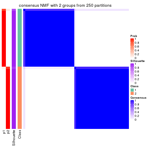
consensus_heatmap(res, k = 3)
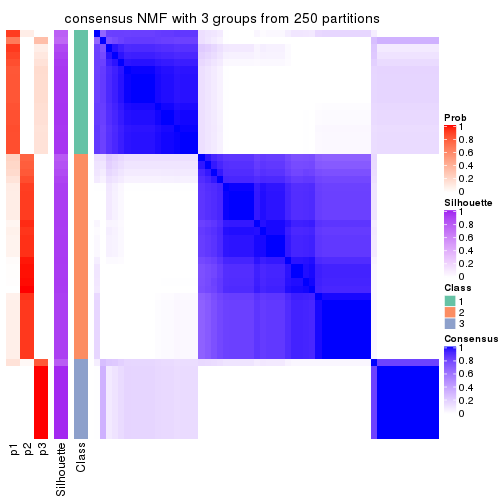
consensus_heatmap(res, k = 4)
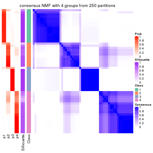
consensus_heatmap(res, k = 5)
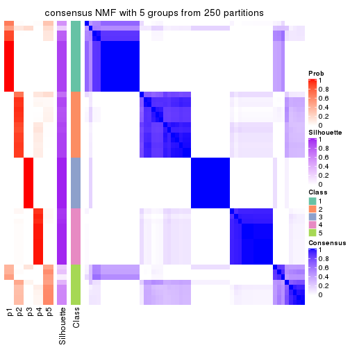
consensus_heatmap(res, k = 6)
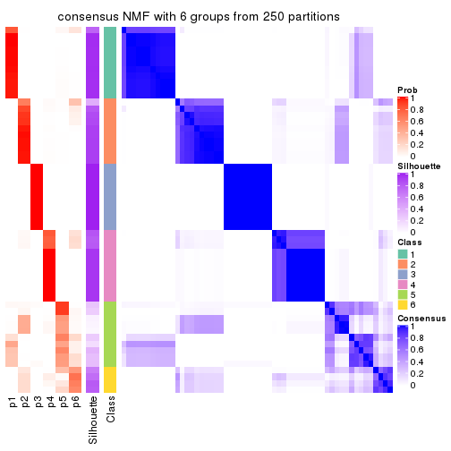
Heatmaps for the membership of samples in all partitions to see how consistent they are:
membership_heatmap(res, k = 2)

membership_heatmap(res, k = 3)
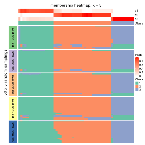
membership_heatmap(res, k = 4)
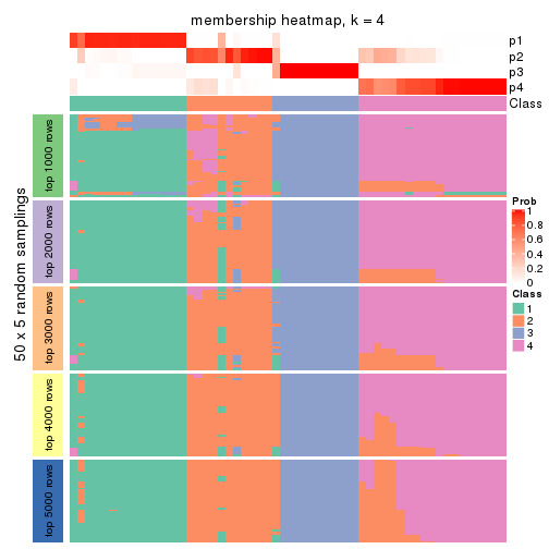
membership_heatmap(res, k = 5)
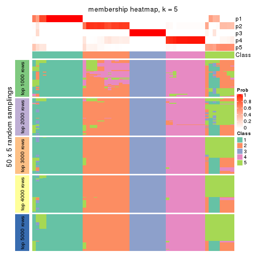
membership_heatmap(res, k = 6)
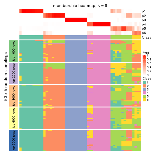
As soon as we have had the classes for columns, we can look for signatures which are significantly different between classes which can be candidate marks for certain classes. Following are the heatmaps for signatures.
Signature heatmaps where rows are scaled:
get_signatures(res, k = 2)
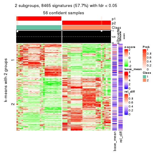
get_signatures(res, k = 3)
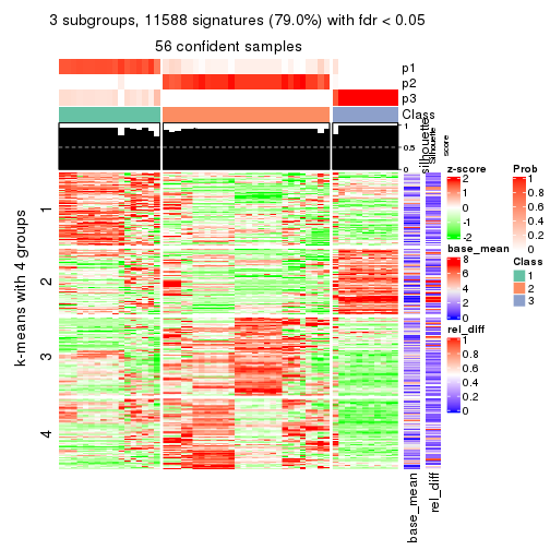
get_signatures(res, k = 4)
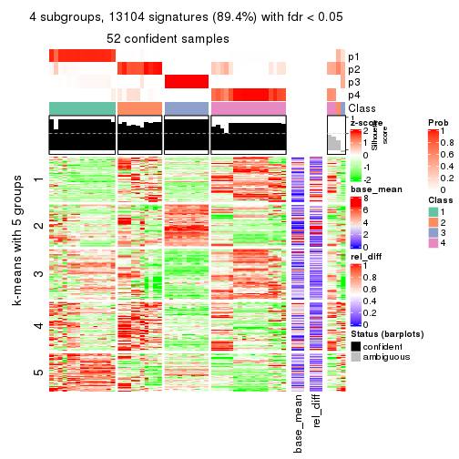
get_signatures(res, k = 5)
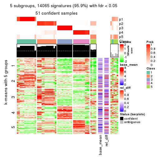
get_signatures(res, k = 6)
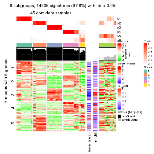
Signature heatmaps where rows are not scaled:
get_signatures(res, k = 2, scale_rows = FALSE)
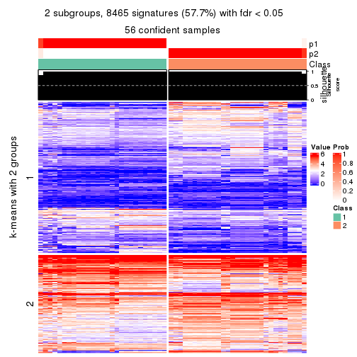
get_signatures(res, k = 3, scale_rows = FALSE)
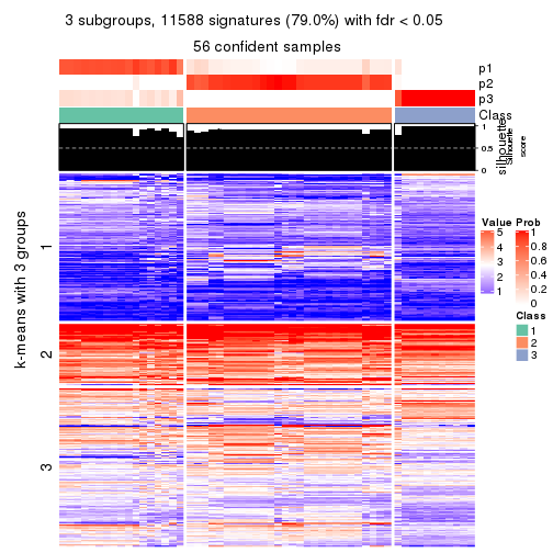
get_signatures(res, k = 4, scale_rows = FALSE)
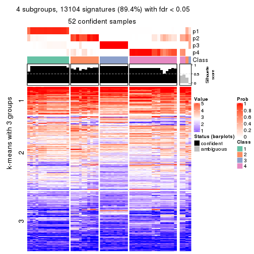
get_signatures(res, k = 5, scale_rows = FALSE)
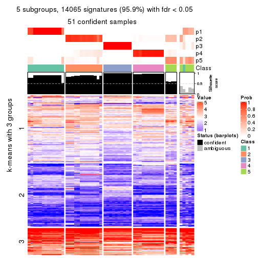
get_signatures(res, k = 6, scale_rows = FALSE)
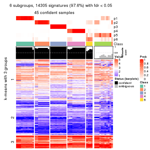
Compare the overlap of signatures from different k:
compare_signatures(res)
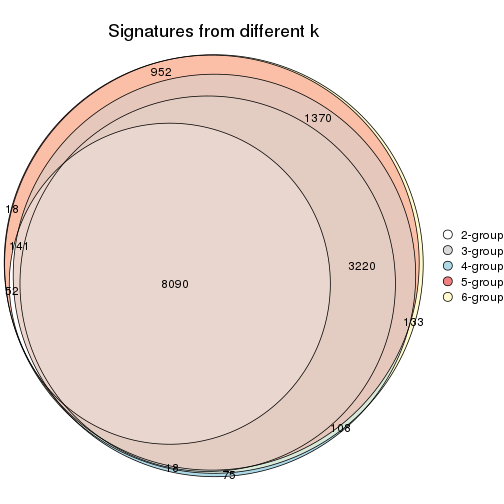
get_signature() returns a data frame invisibly. TO get the list of signatures, the function
call should be assigned to a variable explicitly. In following code, if plot argument is set
to FALSE, no heatmap is plotted while only the differential analysis is performed.
# code only for demonstration
tb = get_signature(res, k = ..., plot = FALSE)
An example of the output of tb is:
#> which_row fdr mean_1 mean_2 scaled_mean_1 scaled_mean_2 km
#> 1 38 0.042760348 8.373488 9.131774 -0.5533452 0.5164555 1
#> 2 40 0.018707592 7.106213 8.469186 -0.6173731 0.5762149 1
#> 3 55 0.019134737 10.221463 11.207825 -0.6159697 0.5749050 1
#> 4 59 0.006059896 5.921854 7.869574 -0.6899429 0.6439467 1
#> 5 60 0.018055526 8.928898 10.211722 -0.6204761 0.5791110 1
#> 6 98 0.009384629 15.714769 14.887706 0.6635654 -0.6193277 2
...
The columns in tb are:
which_row: row indices corresponding to the input matrix.fdr: FDR for the differential test. mean_x: The mean value in group x.scaled_mean_x: The mean value in group x after rows are scaled.km: Row groups if k-means clustering is applied to rows.UMAP plot which shows how samples are separated.
dimension_reduction(res, k = 2, method = "UMAP")
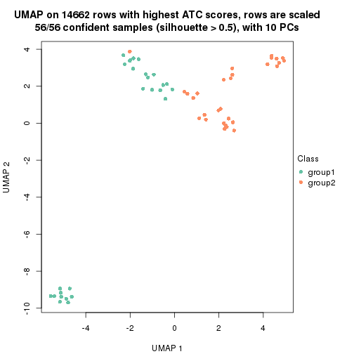
dimension_reduction(res, k = 3, method = "UMAP")
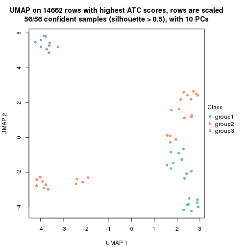
dimension_reduction(res, k = 4, method = "UMAP")
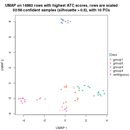
dimension_reduction(res, k = 5, method = "UMAP")
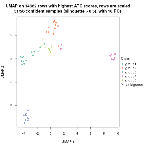
dimension_reduction(res, k = 6, method = "UMAP")
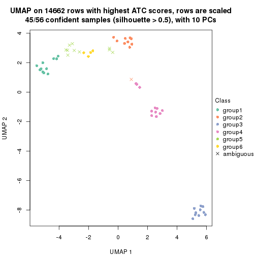
Following heatmap shows how subgroups are split when increasing k:
collect_classes(res)
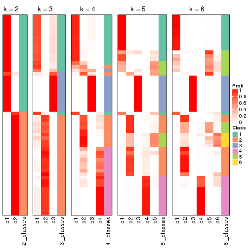
If matrix rows can be associated to genes, consider to use functional_enrichment(res,
...) to perform function enrichment for the signature genes. See this vignette for more detailed explanations.
sessionInfo()
#> R version 3.6.0 (2019-04-26)
#> Platform: x86_64-pc-linux-gnu (64-bit)
#> Running under: CentOS Linux 7 (Core)
#>
#> Matrix products: default
#> BLAS: /usr/lib64/libblas.so.3.4.2
#> LAPACK: /usr/lib64/liblapack.so.3.4.2
#>
#> locale:
#> [1] LC_CTYPE=en_GB.UTF-8 LC_NUMERIC=C LC_TIME=en_GB.UTF-8
#> [4] LC_COLLATE=en_GB.UTF-8 LC_MONETARY=en_GB.UTF-8 LC_MESSAGES=en_GB.UTF-8
#> [7] LC_PAPER=en_GB.UTF-8 LC_NAME=C LC_ADDRESS=C
#> [10] LC_TELEPHONE=C LC_MEASUREMENT=en_GB.UTF-8 LC_IDENTIFICATION=C
#>
#> attached base packages:
#> [1] grid stats graphics grDevices utils datasets methods base
#>
#> other attached packages:
#> [1] genefilter_1.66.0 ComplexHeatmap_2.3.1 markdown_1.1 knitr_1.26
#> [5] GetoptLong_0.1.7 cola_1.3.2
#>
#> loaded via a namespace (and not attached):
#> [1] circlize_0.4.8 shape_1.4.4 xfun_0.11 slam_0.1-46
#> [5] lattice_0.20-38 splines_3.6.0 colorspace_1.4-1 vctrs_0.2.0
#> [9] stats4_3.6.0 blob_1.2.0 XML_3.98-1.20 survival_2.44-1.1
#> [13] rlang_0.4.2 pillar_1.4.2 DBI_1.0.0 BiocGenerics_0.30.0
#> [17] bit64_0.9-7 RColorBrewer_1.1-2 matrixStats_0.55.0 stringr_1.4.0
#> [21] GlobalOptions_0.1.1 evaluate_0.14 memoise_1.1.0 Biobase_2.44.0
#> [25] IRanges_2.18.3 parallel_3.6.0 AnnotationDbi_1.46.1 highr_0.8
#> [29] Rcpp_1.0.3 xtable_1.8-4 backports_1.1.5 S4Vectors_0.22.1
#> [33] annotate_1.62.0 skmeans_0.2-11 bit_1.1-14 microbenchmark_1.4-7
#> [37] brew_1.0-6 impute_1.58.0 rjson_0.2.20 png_0.1-7
#> [41] digest_0.6.23 stringi_1.4.3 polyclip_1.10-0 clue_0.3-57
#> [45] tools_3.6.0 bitops_1.0-6 magrittr_1.5 eulerr_6.0.0
#> [49] RCurl_1.95-4.12 RSQLite_2.1.4 tibble_2.1.3 cluster_2.1.0
#> [53] crayon_1.3.4 pkgconfig_2.0.3 zeallot_0.1.0 Matrix_1.2-17
#> [57] xml2_1.2.2 httr_1.4.1 R6_2.4.1 mclust_5.4.5
#> [61] compiler_3.6.0