
Date: 2019-12-25 23:26:32 CET, cola version: 1.3.2
Document is loading...
All available functions which can be applied to this res_list object:
res_list
#> A 'ConsensusPartitionList' object with 24 methods.
#>   On a matrix with 10126 rows and 62 columns.
#>   Top rows are extracted by 'SD, CV, MAD, ATC' methods.
#>   Subgroups are detected by 'hclust, kmeans, skmeans, pam, mclust, NMF' method.
#>   Number of partitions are tried for k = 2, 3, 4, 5, 6.
#>   Performed in total 30000 partitions by row resampling.
#>
#> Following methods can be applied to this 'ConsensusPartitionList' object:
#>  [1] "cola_report"           "collect_classes"       "collect_plots"         "collect_stats"
#>  [5] "colnames"              "functional_enrichment" "get_anno_col"          "get_anno"
#>  [9] "get_classes"           "get_matrix"            "get_membership"        "get_stats"
#> [13] "is_best_k"             "is_stable_k"           "ncol"                  "nrow"
#> [17] "rownames"              "show"                  "suggest_best_k"        "test_to_known_factors"
#> [21] "top_rows_heatmap"      "top_rows_overlap"
#>
#> You can get result for a single method by, e.g. object["SD", "hclust"] or object["SD:hclust"]
#> or a subset of methods by object[c("SD", "CV")], c("hclust", "kmeans")]
The call of run_all_consensus_partition_methods() was:
#> run_all_consensus_partition_methods(data = mat, mc.cores = 4)
Dimension of the input matrix:
mat = get_matrix(res_list)
dim(mat)
#> [1] 10126 62
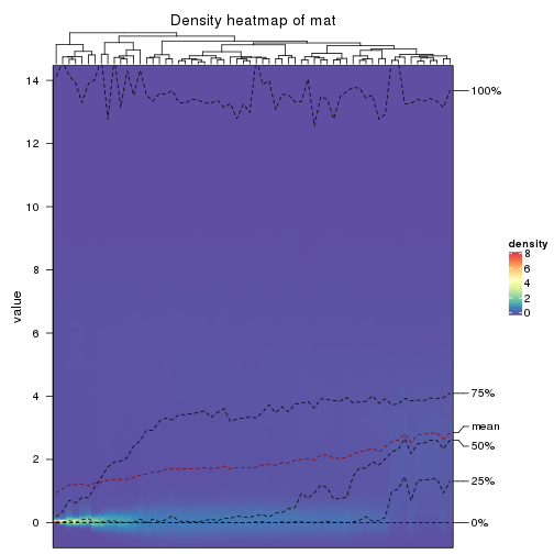
The density distribution for each sample is visualized as in one column in the following heatmap. The clustering is based on the distance which is the Kolmogorov-Smirnov statistic between two distributions.
library(ComplexHeatmap)
densityHeatmap(mat, ylab = "value", cluster_columns = TRUE, show_column_names = FALSE,
    mc.cores = 4)
Folowing table shows the best k (number of partitions) for each combination
of top-value methods and partition methods. Clicking on the method name in
the table goes to the section for a single combination of methods.
The cola vignette explains the definition of the metrics used for determining the best number of partitions.
suggest_best_k(res_list)
| The best k | 1-PAC | Mean silhouette | Concordance | Optional k | ||
|---|---|---|---|---|---|---|
| CV:skmeans | 2 | 1.000 | 0.975 | 0.990 | ** | |
| MAD:skmeans | 2 | 1.000 | 0.963 | 0.986 | ** | |
| CV:kmeans | 3 | 0.972 | 0.938 | 0.972 | ** | 2 |
| CV:pam | 2 | 0.966 | 0.971 | 0.984 | ** | |
| SD:pam | 3 | 0.964 | 0.958 | 0.982 | ** | 2 |
| CV:hclust | 3 | 0.933 | 0.963 | 0.978 | * | 2 |
| ATC:kmeans | 2 | 0.932 | 0.875 | 0.953 | * | |
| ATC:skmeans | 2 | 0.932 | 0.921 | 0.969 | * | |
| ATC:pam | 2 | 0.932 | 0.890 | 0.960 | * | |
| SD:hclust | 2 | 0.925 | 0.947 | 0.972 | * | |
| CV:mclust | 2 | 0.901 | 0.941 | 0.971 | * | |
| SD:NMF | 2 | 0.900 | 0.910 | 0.961 | ||
| MAD:NMF | 2 | 0.899 | 0.934 | 0.971 | ||
| MAD:kmeans | 4 | 0.878 | 0.811 | 0.893 | ||
| SD:skmeans | 3 | 0.862 | 0.885 | 0.949 | ||
| ATC:hclust | 3 | 0.831 | 0.945 | 0.969 | ||
| SD:kmeans | 4 | 0.772 | 0.794 | 0.870 | ||
| MAD:pam | 3 | 0.766 | 0.874 | 0.935 | ||
| ATC:mclust | 3 | 0.658 | 0.799 | 0.882 | ||
| MAD:mclust | 3 | 0.501 | 0.750 | 0.797 | ||
| SD:mclust | 3 | 0.483 | 0.834 | 0.870 | ||
| CV:NMF | 2 | 0.479 | 0.757 | 0.887 | ||
| MAD:hclust | 2 | 0.458 | 0.870 | 0.914 | ||
| ATC:NMF | 3 | 0.425 | 0.788 | 0.857 |
**: 1-PAC > 0.95, *: 1-PAC > 0.9
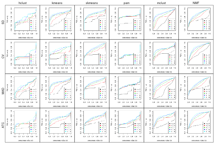
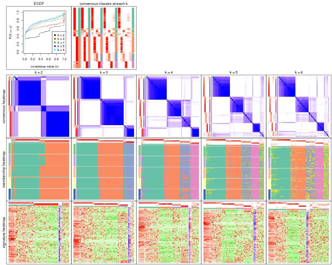
Cumulative distribution function curves of consensus matrix for all methods.
collect_plots(res_list, fun = plot_ecdf)
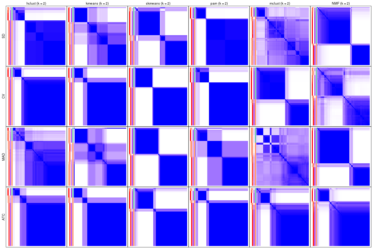
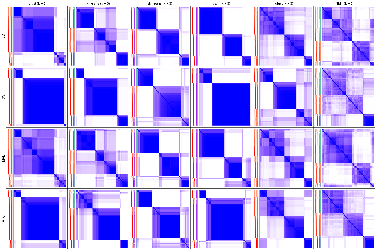
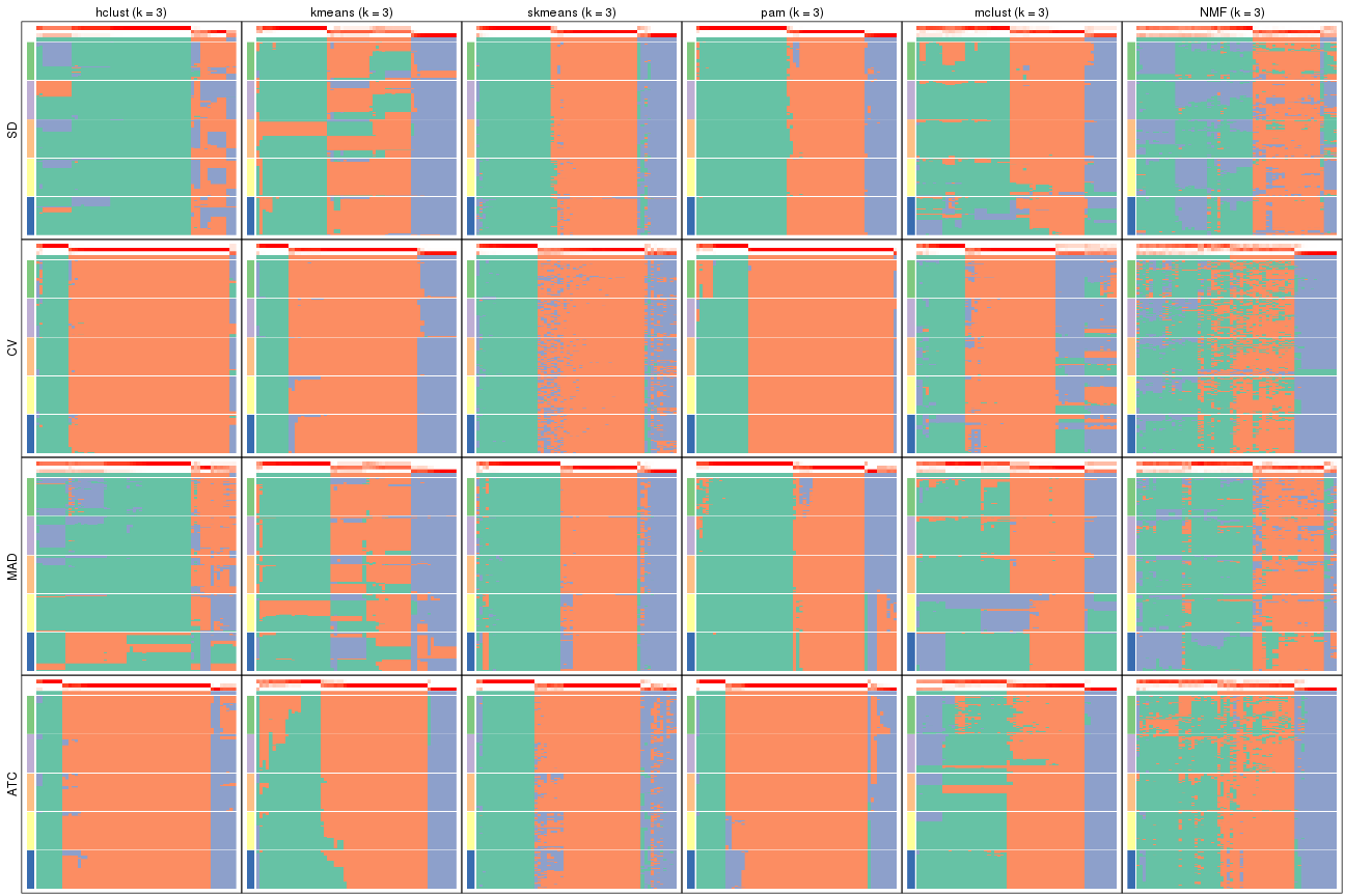
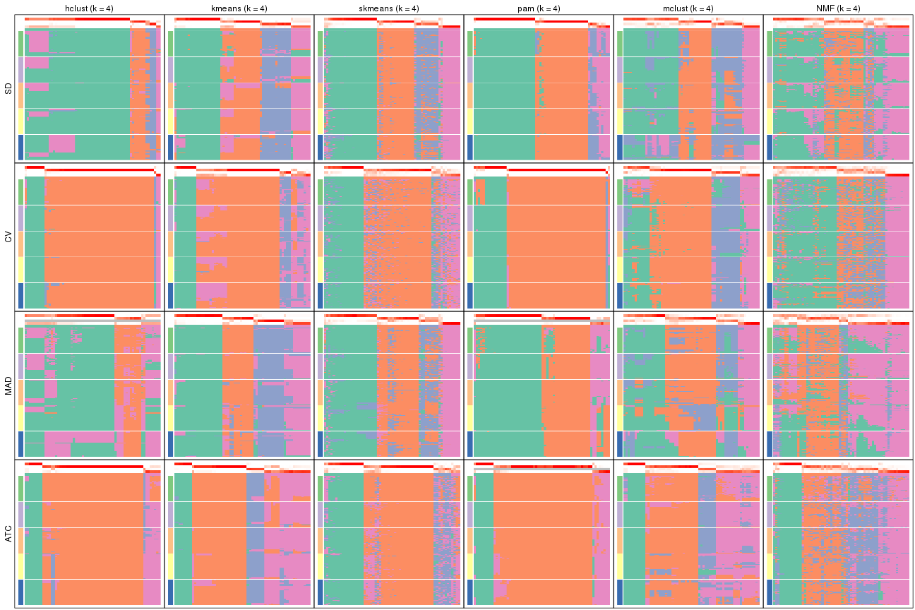
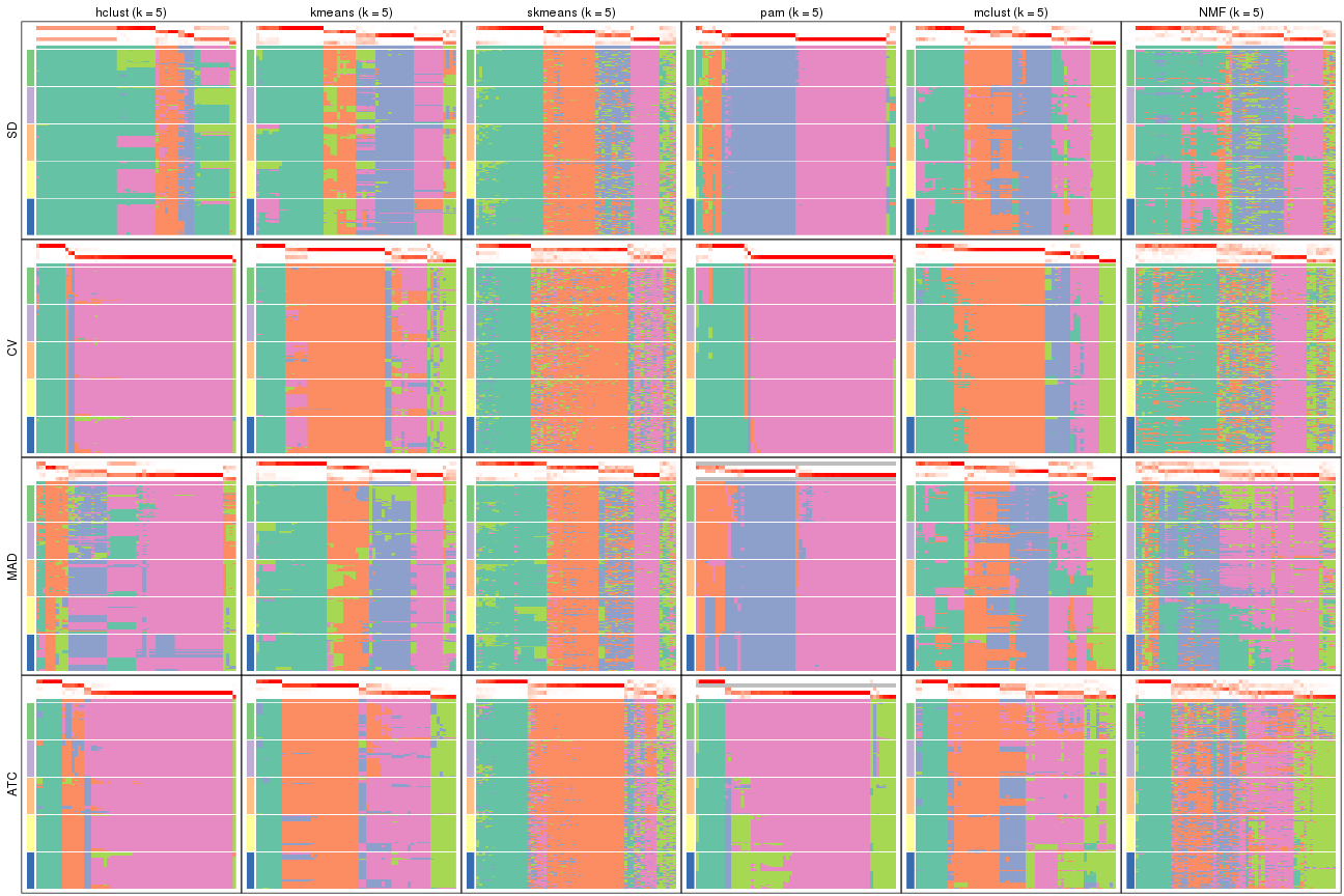
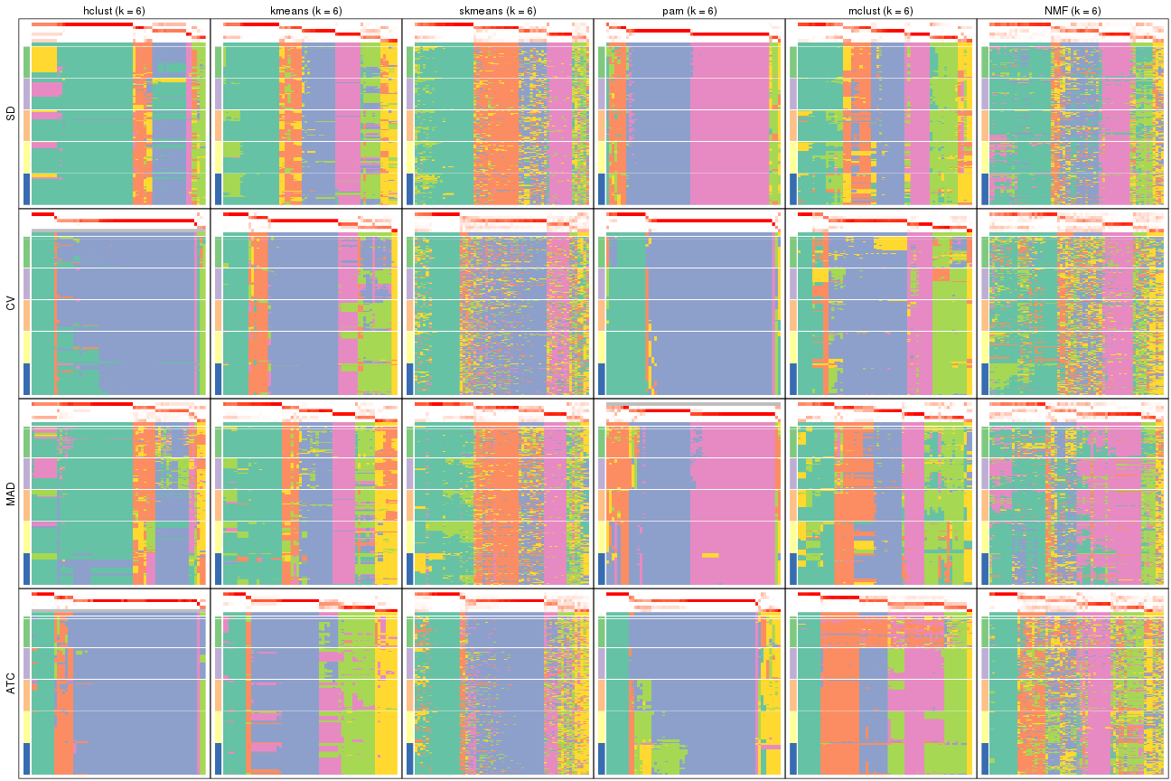
Consensus heatmaps for all methods. (What is a consensus heatmap?)
collect_plots(res_list, k = 2, fun = consensus_heatmap, mc.cores = 4)
collect_plots(res_list, k = 3, fun = consensus_heatmap, mc.cores = 4)
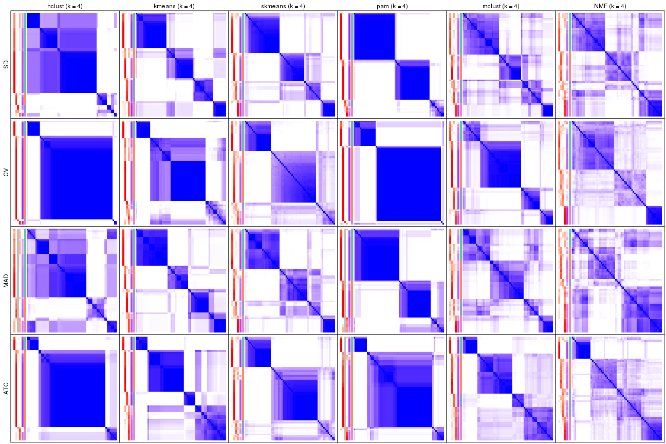
collect_plots(res_list, k = 4, fun = consensus_heatmap, mc.cores = 4)
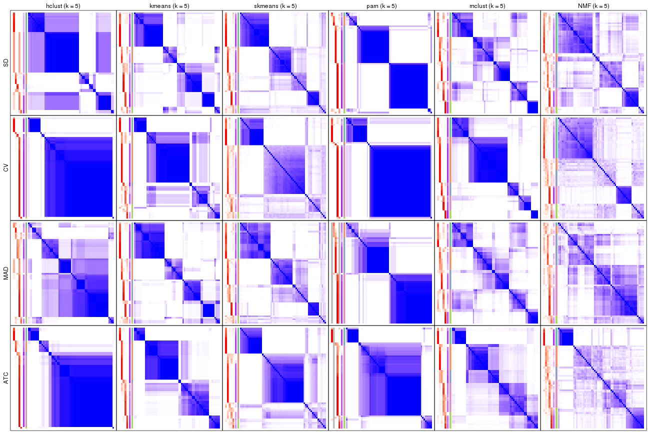
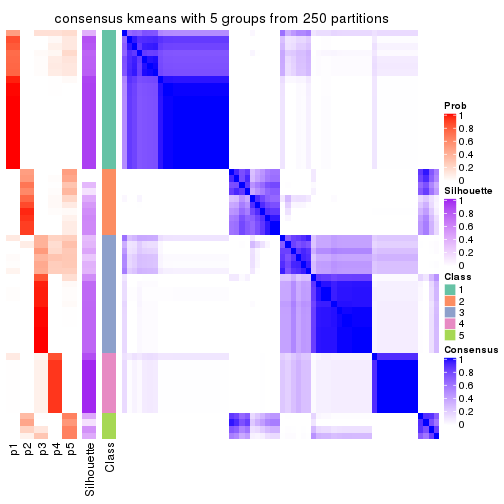
collect_plots(res_list, k = 5, fun = consensus_heatmap, mc.cores = 4)
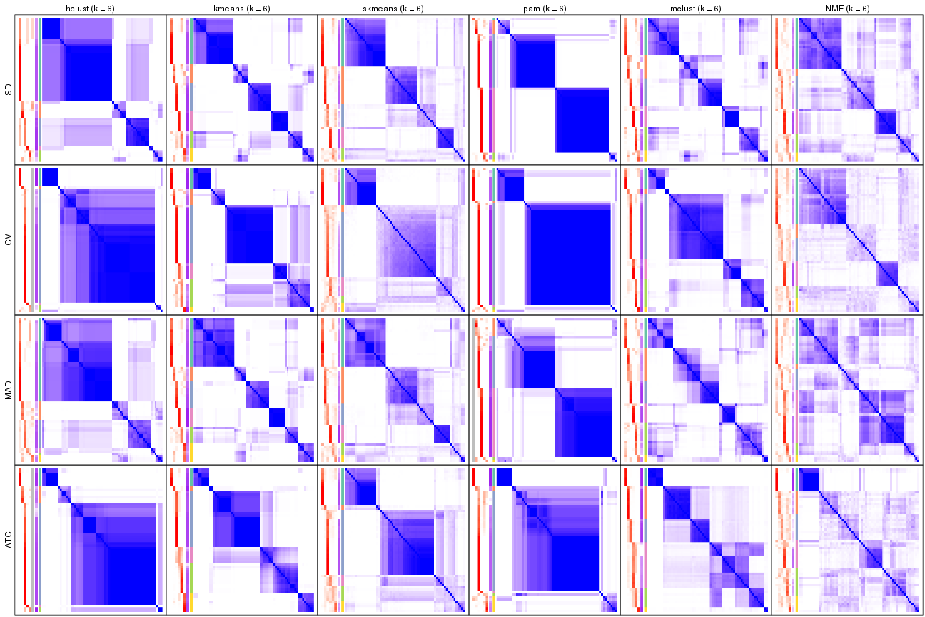
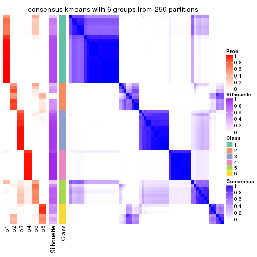
collect_plots(res_list, k = 6, fun = consensus_heatmap, mc.cores = 4)
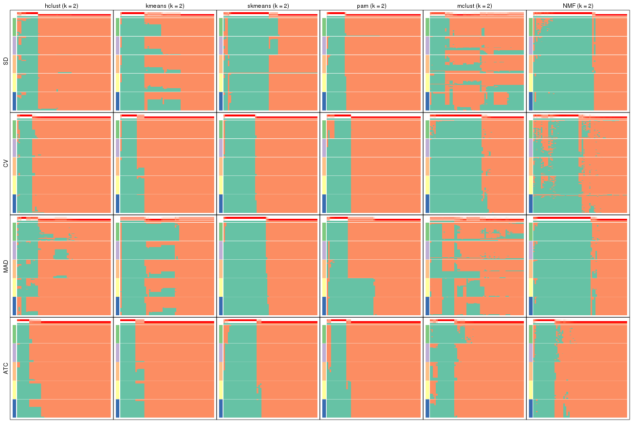
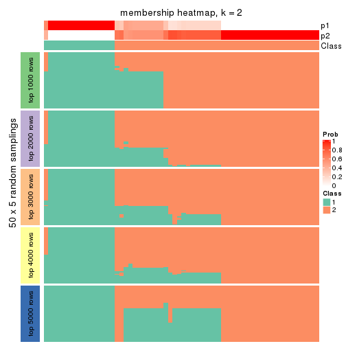
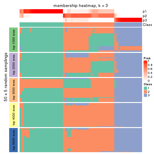
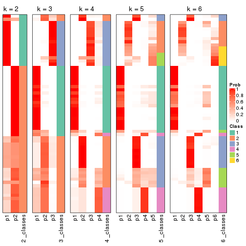
Membership heatmaps for all methods. (What is a membership heatmap?)
collect_plots(res_list, k = 2, fun = membership_heatmap, mc.cores = 4)
collect_plots(res_list, k = 3, fun = membership_heatmap, mc.cores = 4)
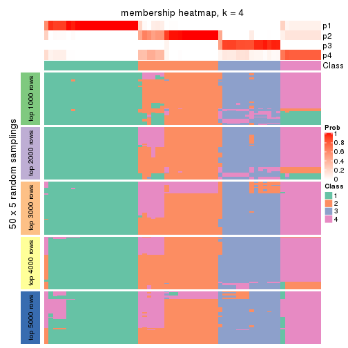
collect_plots(res_list, k = 4, fun = membership_heatmap, mc.cores = 4)
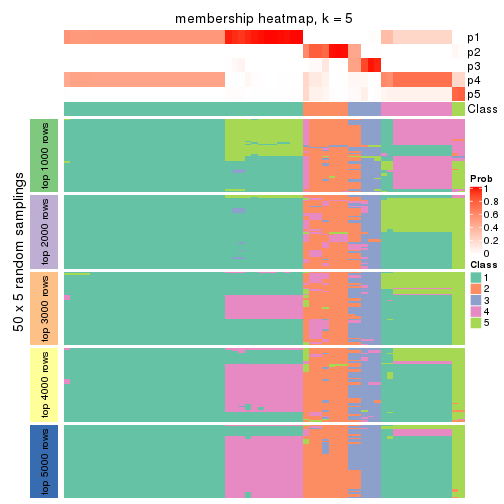
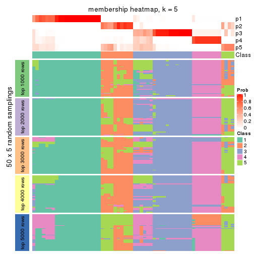
collect_plots(res_list, k = 5, fun = membership_heatmap, mc.cores = 4)
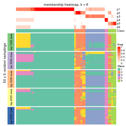
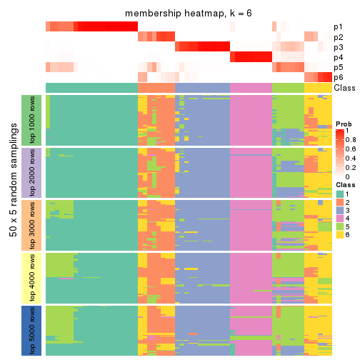
collect_plots(res_list, k = 6, fun = membership_heatmap, mc.cores = 4)
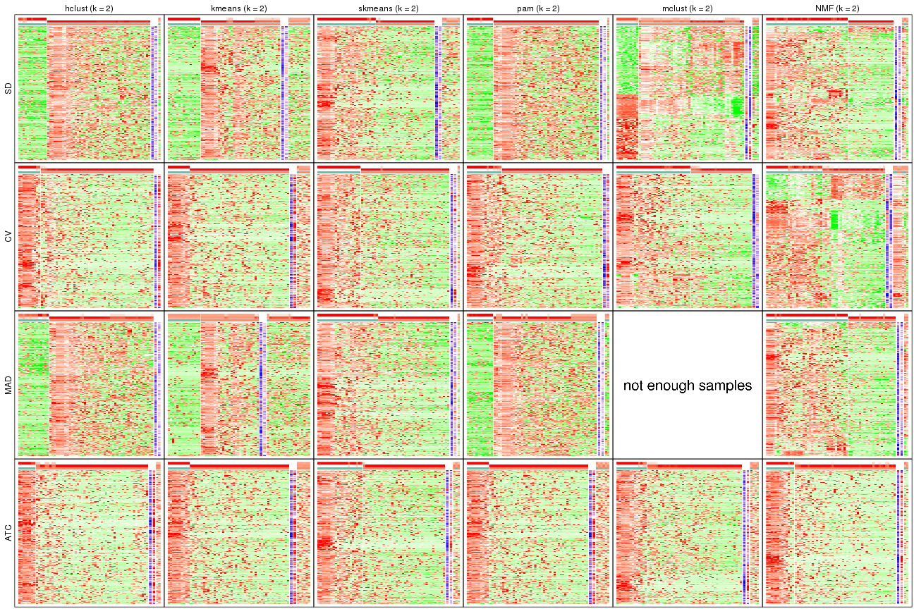
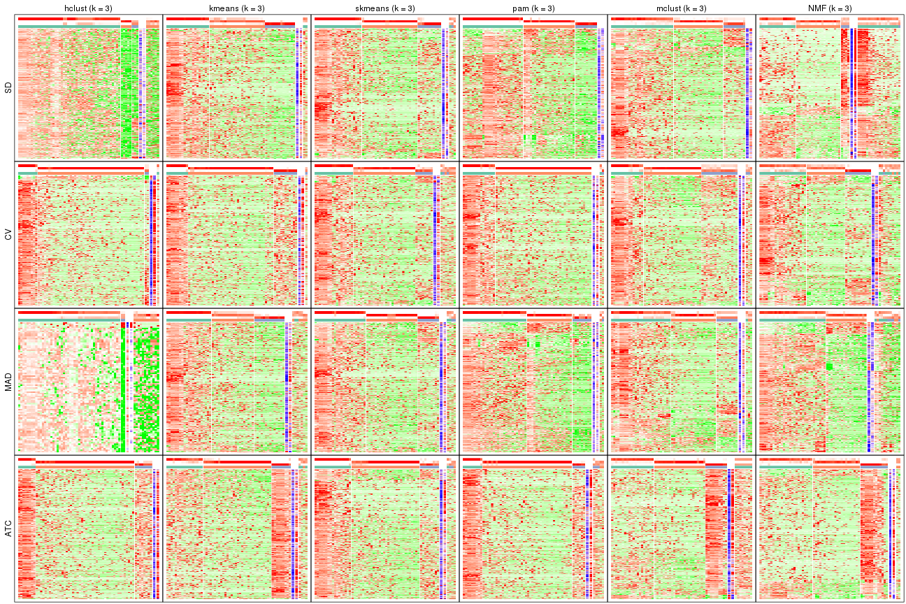
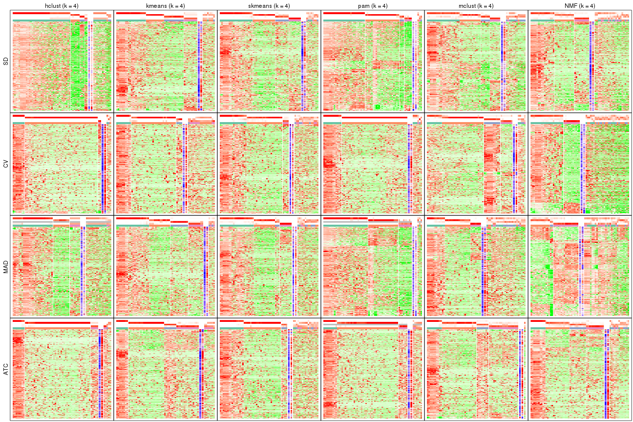
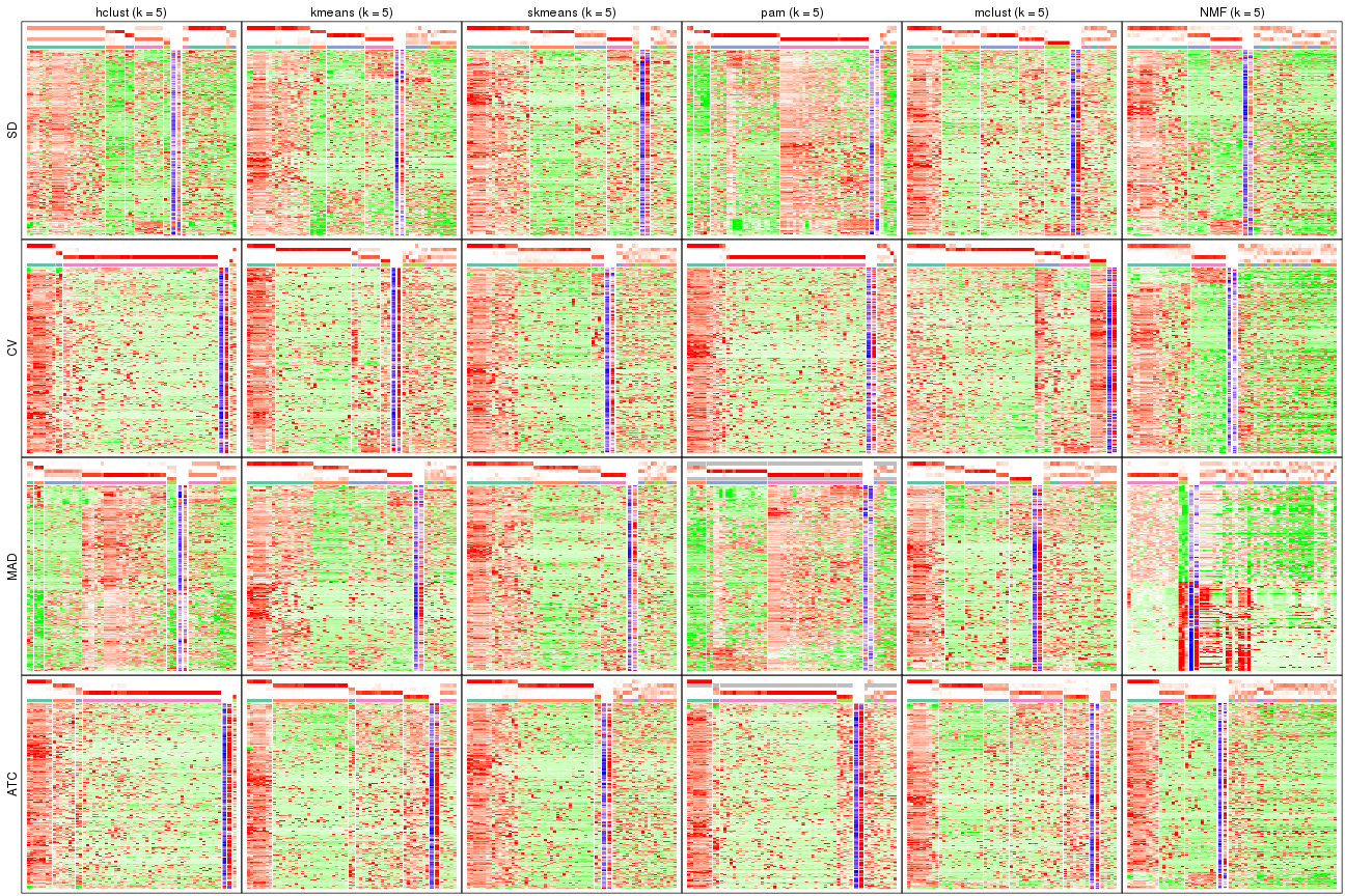
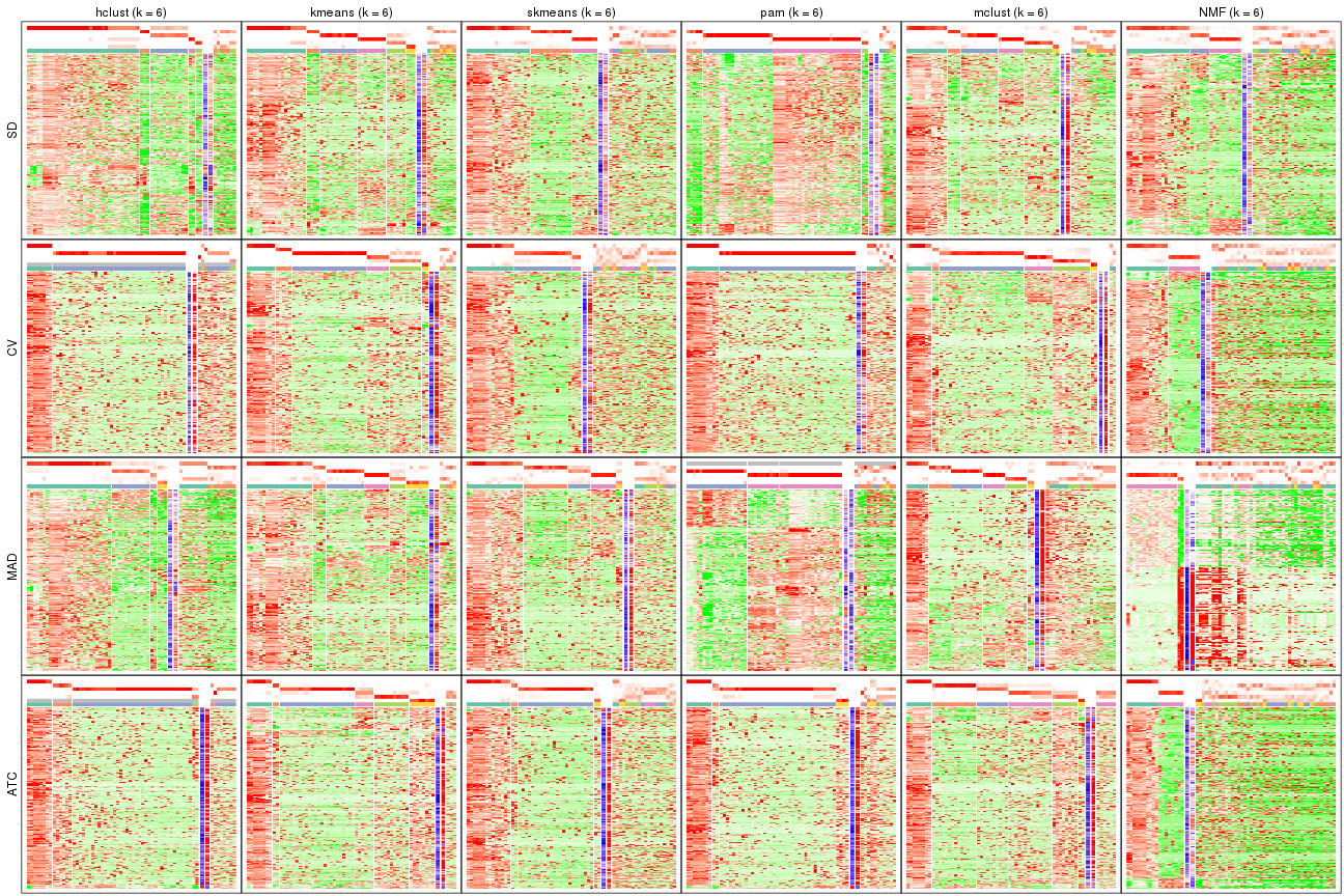
Signature heatmaps for all methods. (What is a signature heatmap?)
Note in following heatmaps, rows are scaled.
collect_plots(res_list, k = 2, fun = get_signatures, mc.cores = 4)
collect_plots(res_list, k = 3, fun = get_signatures, mc.cores = 4)
collect_plots(res_list, k = 4, fun = get_signatures, mc.cores = 4)
collect_plots(res_list, k = 5, fun = get_signatures, mc.cores = 4)
collect_plots(res_list, k = 6, fun = get_signatures, mc.cores = 4)
The statistics used for measuring the stability of consensus partitioning. (How are they defined?)
get_stats(res_list, k = 2)
#>             k 1-PAC mean_silhouette concordance area_increased  Rand Jaccard
#> SD:NMF      2 0.900           0.910       0.961          0.477 0.526   0.526
#> CV:NMF      2 0.479           0.757       0.887          0.494 0.492   0.492
#> MAD:NMF     2 0.899           0.934       0.971          0.475 0.518   0.518
#> ATC:NMF     2 0.831           0.912       0.961          0.378 0.645   0.645
#> SD:skmeans  2 0.751           0.842       0.930          0.506 0.492   0.492
#> CV:skmeans  2 1.000           0.975       0.990          0.454 0.545   0.545
#> MAD:skmeans 2 1.000           0.963       0.986          0.504 0.497   0.497
#> ATC:skmeans 2 0.932           0.921       0.969          0.463 0.535   0.535
#> SD:mclust   2 0.185           0.661       0.777          0.403 0.725   0.725
#> CV:mclust   2 0.901           0.941       0.971          0.499 0.497   0.497
#> MAD:mclust  2 0.192           0.381       0.736          0.372 0.611   0.611
#> ATC:mclust  2 0.749           0.861       0.943          0.383 0.611   0.611
#> SD:kmeans   2 0.445           0.773       0.875          0.430 0.611   0.611
#> CV:kmeans   2 0.932           0.879       0.957          0.332 0.703   0.703
#> MAD:kmeans  2 0.454           0.582       0.803          0.450 0.611   0.611
#> ATC:kmeans  2 0.932           0.875       0.953          0.331 0.725   0.725
#> SD:pam      2 1.000           0.967       0.986          0.321 0.683   0.683
#> CV:pam      2 0.966           0.971       0.984          0.372 0.611   0.611
#> MAD:pam     2 0.563           0.728       0.872          0.407 0.645   0.645
#> ATC:pam     2 0.932           0.890       0.960          0.329 0.663   0.663
#> SD:hclust   2 0.925           0.947       0.972          0.336 0.645   0.645
#> CV:hclust   2 1.000           0.970       0.986          0.277 0.725   0.725
#> MAD:hclust  2 0.458           0.870       0.914          0.322 0.645   0.645
#> ATC:hclust  2 0.869           0.904       0.957          0.277 0.772   0.772
get_stats(res_list, k = 3)
#>             k 1-PAC mean_silhouette concordance area_increased  Rand Jaccard
#> SD:NMF      3 0.442           0.511       0.701         0.3317 0.918   0.844
#> CV:NMF      3 0.267           0.642       0.755         0.3093 0.648   0.414
#> MAD:NMF     3 0.459           0.625       0.792         0.2641 0.937   0.878
#> ATC:NMF     3 0.425           0.788       0.857         0.7118 0.677   0.508
#> SD:skmeans  3 0.862           0.885       0.949         0.2733 0.772   0.576
#> CV:skmeans  3 0.701           0.797       0.896         0.3566 0.832   0.696
#> MAD:skmeans 3 0.847           0.844       0.937         0.2840 0.835   0.675
#> ATC:skmeans 3 0.721           0.816       0.916         0.3236 0.825   0.681
#> SD:mclust   3 0.483           0.834       0.870         0.5044 0.647   0.513
#> CV:mclust   3 0.569           0.769       0.848         0.2409 0.849   0.696
#> MAD:mclust  3 0.501           0.750       0.797         0.6298 0.618   0.440
#> ATC:mclust  3 0.658           0.799       0.882         0.6640 0.619   0.441
#> SD:kmeans   3 0.582           0.784       0.833         0.4771 0.681   0.498
#> CV:kmeans   3 0.972           0.938       0.972         0.5946 0.756   0.656
#> MAD:kmeans  3 0.494           0.749       0.800         0.4139 0.681   0.498
#> ATC:kmeans  3 0.676           0.822       0.916         0.7367 0.654   0.529
#> SD:pam      3 0.964           0.958       0.982         0.9594 0.640   0.491
#> CV:pam      3 0.933           0.930       0.980         0.0616 0.976   0.961
#> MAD:pam     3 0.766           0.874       0.935         0.4786 0.655   0.495
#> ATC:pam     3 0.854           0.853       0.947         0.4084 0.854   0.783
#> SD:hclust   3 0.684           0.760       0.840         0.3493 0.983   0.973
#> CV:hclust   3 0.933           0.963       0.978         0.1754 0.947   0.927
#> MAD:hclust  3 0.381           0.580       0.760         0.5087 0.987   0.980
#> ATC:hclust  3 0.831           0.945       0.969         0.4741 0.805   0.748
get_stats(res_list, k = 4)
#>             k 1-PAC mean_silhouette concordance area_increased  Rand Jaccard
#> SD:NMF      4 0.426           0.516       0.739         0.1051 0.746   0.486
#> CV:NMF      4 0.452           0.519       0.727         0.1209 0.872   0.675
#> MAD:NMF     4 0.407           0.410       0.681         0.1194 0.794   0.583
#> ATC:NMF     4 0.455           0.609       0.757         0.1573 0.827   0.544
#> SD:skmeans  4 0.778           0.780       0.883         0.1305 0.882   0.681
#> CV:skmeans  4 0.552           0.645       0.817         0.1168 0.950   0.874
#> MAD:skmeans 4 0.647           0.671       0.834         0.1201 0.864   0.646
#> ATC:skmeans 4 0.730           0.616       0.833         0.0917 0.935   0.840
#> SD:mclust   4 0.560           0.642       0.793         0.1580 0.846   0.616
#> CV:mclust   4 0.730           0.783       0.873         0.1152 0.928   0.798
#> MAD:mclust  4 0.499           0.566       0.748         0.1703 0.900   0.730
#> ATC:mclust  4 0.494           0.824       0.839         0.1048 0.915   0.771
#> SD:kmeans   4 0.772           0.794       0.870         0.1481 0.909   0.736
#> CV:kmeans   4 0.656           0.640       0.850         0.1632 0.934   0.862
#> MAD:kmeans  4 0.878           0.811       0.893         0.1535 0.899   0.709
#> ATC:kmeans  4 0.783           0.838       0.905         0.1845 0.783   0.526
#> SD:pam      4 0.902           0.892       0.953         0.0227 0.987   0.966
#> CV:pam      4 0.894           0.872       0.970         0.0435 0.992   0.986
#> MAD:pam     4 0.770           0.841       0.909         0.0268 0.979   0.947
#> ATC:pam     4 0.745           0.818       0.906         0.0948 0.973   0.951
#> SD:hclust   4 0.552           0.733       0.865         0.1050 0.980   0.968
#> CV:hclust   4 0.999           0.943       0.981         0.0622 0.995   0.993
#> MAD:hclust  4 0.469           0.498       0.727         0.1980 0.820   0.723
#> ATC:hclust  4 0.718           0.862       0.948         0.0708 0.996   0.994
get_stats(res_list, k = 5)
#>             k 1-PAC mean_silhouette concordance area_increased  Rand Jaccard
#> SD:NMF      5 0.473           0.486       0.722        0.05570 0.901   0.693
#> CV:NMF      5 0.503           0.447       0.653        0.06675 0.889   0.662
#> MAD:NMF     5 0.382           0.304       0.628        0.06218 0.851   0.637
#> ATC:NMF     5 0.532           0.449       0.682        0.07123 0.897   0.621
#> SD:skmeans  5 0.711           0.744       0.837        0.05550 0.939   0.783
#> CV:skmeans  5 0.544           0.540       0.752        0.06951 0.971   0.919
#> MAD:skmeans 5 0.646           0.669       0.794        0.06244 0.922   0.736
#> ATC:skmeans 5 0.700           0.595       0.798        0.05149 0.936   0.827
#> SD:mclust   5 0.714           0.677       0.843        0.12472 0.859   0.541
#> CV:mclust   5 0.862           0.875       0.932        0.05389 0.979   0.928
#> MAD:mclust  5 0.611           0.532       0.747        0.09063 0.850   0.511
#> ATC:mclust  5 0.615           0.683       0.781        0.07424 0.905   0.676
#> SD:kmeans   5 0.737           0.684       0.809        0.06183 0.979   0.918
#> CV:kmeans   5 0.690           0.666       0.851        0.09671 0.840   0.641
#> MAD:kmeans  5 0.789           0.703       0.833        0.05397 0.973   0.895
#> ATC:kmeans  5 0.825           0.833       0.901        0.06328 0.957   0.862
#> SD:pam      5 0.915           0.853       0.934        0.01131 0.985   0.957
#> CV:pam      5 0.868           0.873       0.966        0.03569 0.977   0.960
#> MAD:pam     5 0.751           0.828       0.898        0.00916 1.000   1.000
#> ATC:pam     5 0.669           0.684       0.874        0.07376 0.955   0.918
#> SD:hclust   5 0.566           0.575       0.713        0.14017 0.785   0.649
#> CV:hclust   5 0.975           0.925       0.976        0.08097 0.974   0.961
#> MAD:hclust  5 0.437           0.628       0.761        0.07159 0.857   0.718
#> ATC:hclust  5 0.811           0.897       0.945        0.06946 0.953   0.919
get_stats(res_list, k = 6)
#>             k 1-PAC mean_silhouette concordance area_increased  Rand Jaccard
#> SD:NMF      6 0.529           0.509       0.716        0.03686 0.928   0.741
#> CV:NMF      6 0.522           0.380       0.607        0.04741 0.936   0.757
#> MAD:NMF     6 0.446           0.359       0.657        0.04314 0.791   0.488
#> ATC:NMF     6 0.580           0.408       0.625        0.04301 0.870   0.466
#> SD:skmeans  6 0.731           0.610       0.790        0.03261 0.995   0.977
#> CV:skmeans  6 0.553           0.463       0.692        0.04455 0.949   0.846
#> MAD:skmeans 6 0.646           0.600       0.726        0.03668 0.974   0.891
#> ATC:skmeans 6 0.623           0.588       0.775        0.04408 0.955   0.858
#> SD:mclust   6 0.724           0.618       0.813        0.03636 0.950   0.761
#> CV:mclust   6 0.802           0.808       0.874        0.02683 0.979   0.926
#> MAD:mclust  6 0.695           0.573       0.773        0.04917 0.957   0.790
#> ATC:mclust  6 0.661           0.748       0.812        0.03403 0.941   0.747
#> SD:kmeans   6 0.840           0.734       0.842        0.04066 0.935   0.737
#> CV:kmeans   6 0.774           0.832       0.872        0.07066 0.875   0.630
#> MAD:kmeans  6 0.764           0.758       0.822        0.03770 0.940   0.752
#> ATC:kmeans  6 0.768           0.829       0.864        0.04721 0.952   0.826
#> SD:pam      6 0.912           0.855       0.947        0.00861 0.997   0.992
#> CV:pam      6 0.808           0.815       0.959        0.03828 0.993   0.987
#> MAD:pam     6 0.722           0.723       0.893        0.01525 0.973   0.930
#> ATC:pam     6 0.680           0.605       0.858        0.02413 0.986   0.972
#> SD:hclust   6 0.546           0.737       0.807        0.07361 0.696   0.441
#> CV:hclust   6 0.647           0.753       0.884        0.26477 0.995   0.992
#> MAD:hclust  6 0.470           0.636       0.758        0.05925 0.994   0.984
#> ATC:hclust  6 0.728           0.784       0.900        0.11124 1.000   1.000
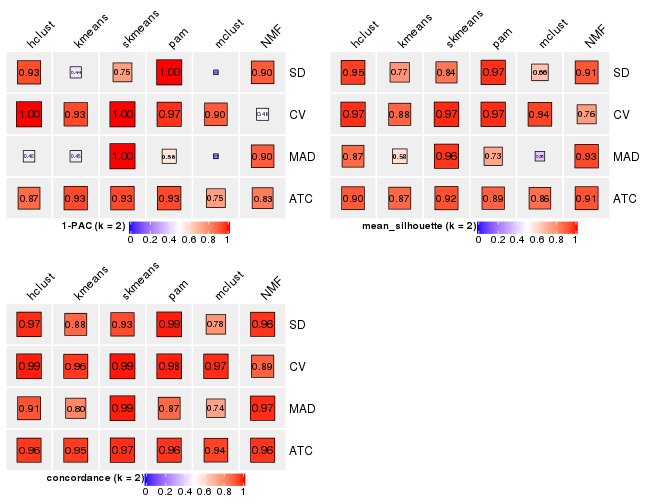
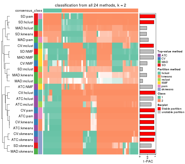
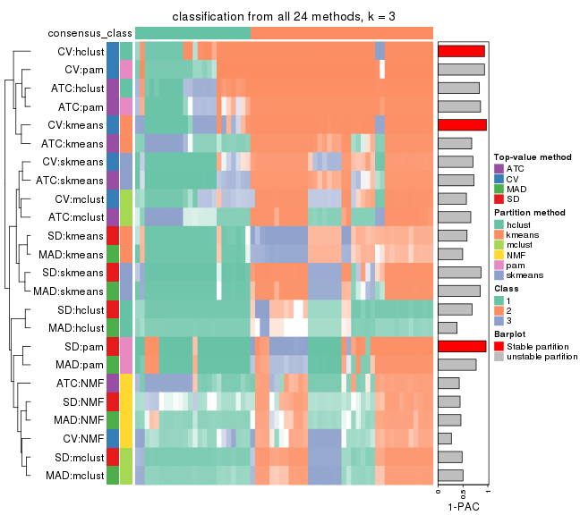
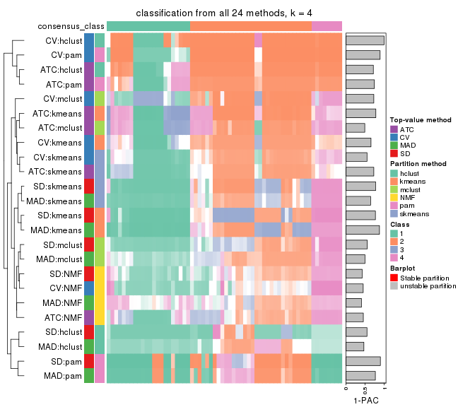
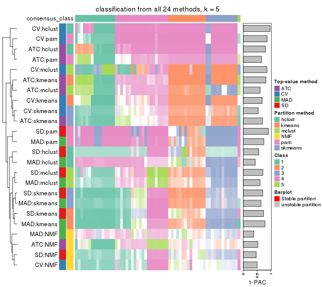
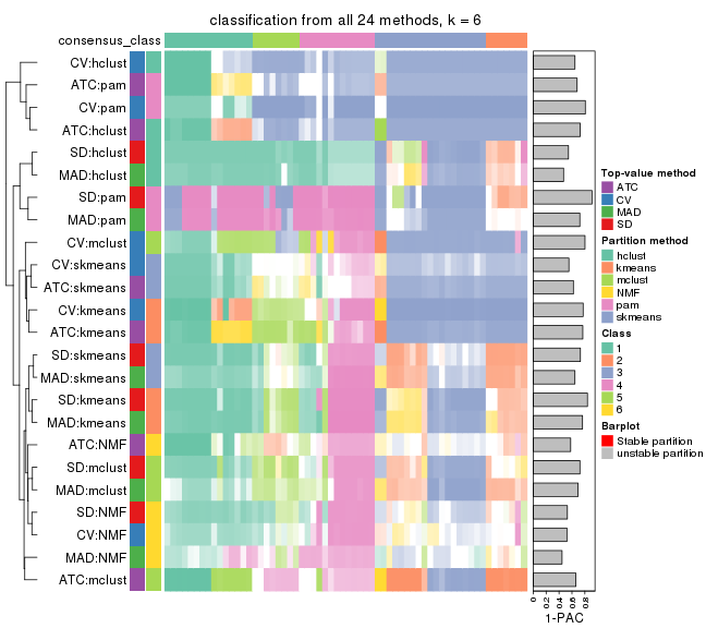
Following heatmap plots the partition for each combination of methods and the lightness correspond to the silhouette scores for samples in each method. On top the consensus subgroup is inferred from all methods by taking the mean silhouette scores as weight.
collect_stats(res_list, k = 2)
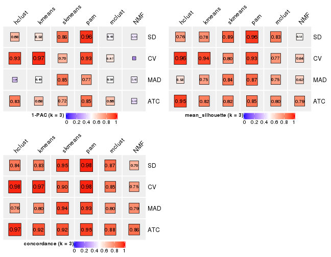
collect_stats(res_list, k = 3)
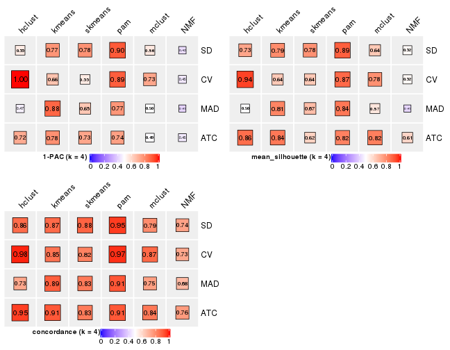
collect_stats(res_list, k = 4)
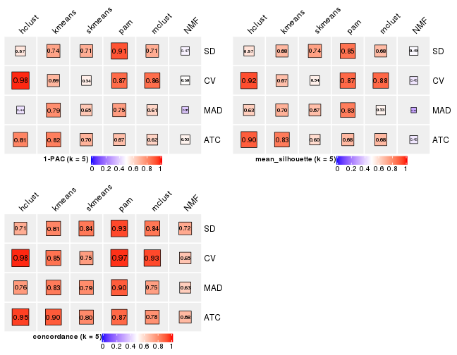
collect_stats(res_list, k = 5)
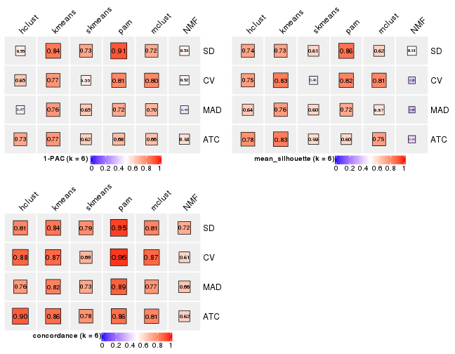
collect_stats(res_list, k = 6)
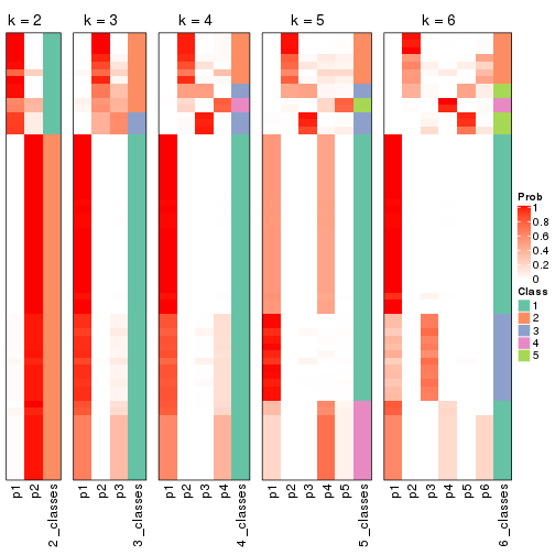
Collect partitions from all methods:
collect_classes(res_list, k = 2)
collect_classes(res_list, k = 3)
collect_classes(res_list, k = 4)
collect_classes(res_list, k = 5)
collect_classes(res_list, k = 6)
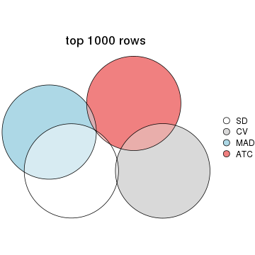
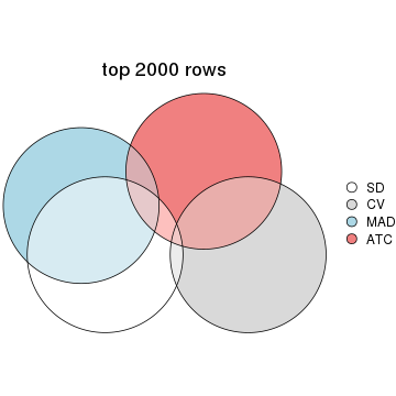
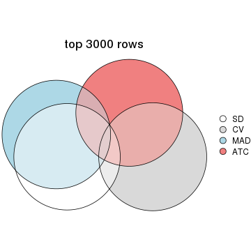
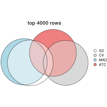
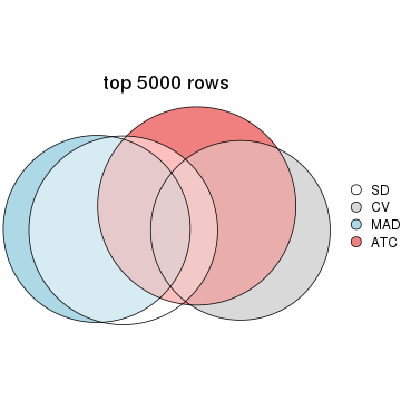
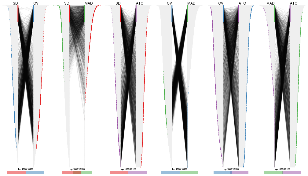
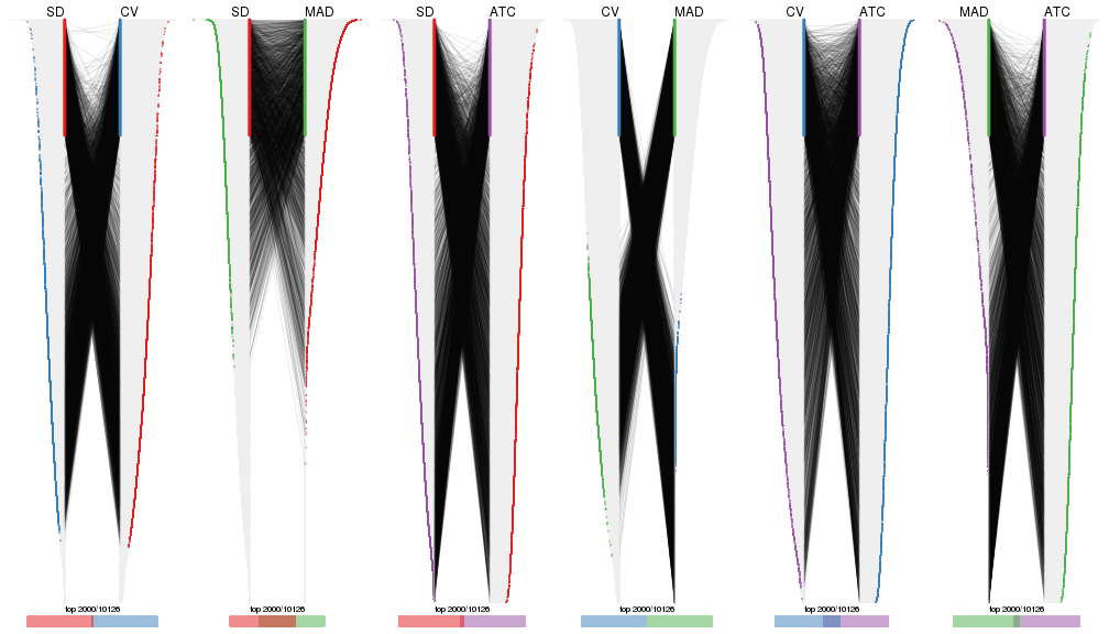
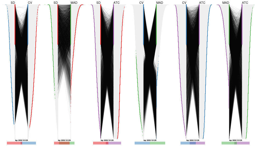
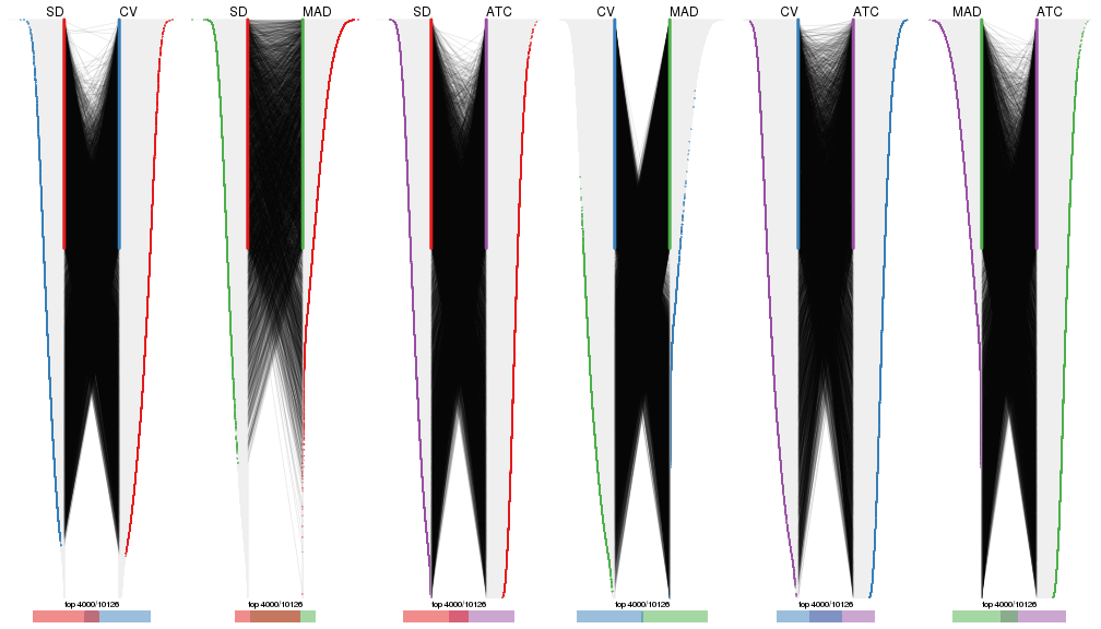
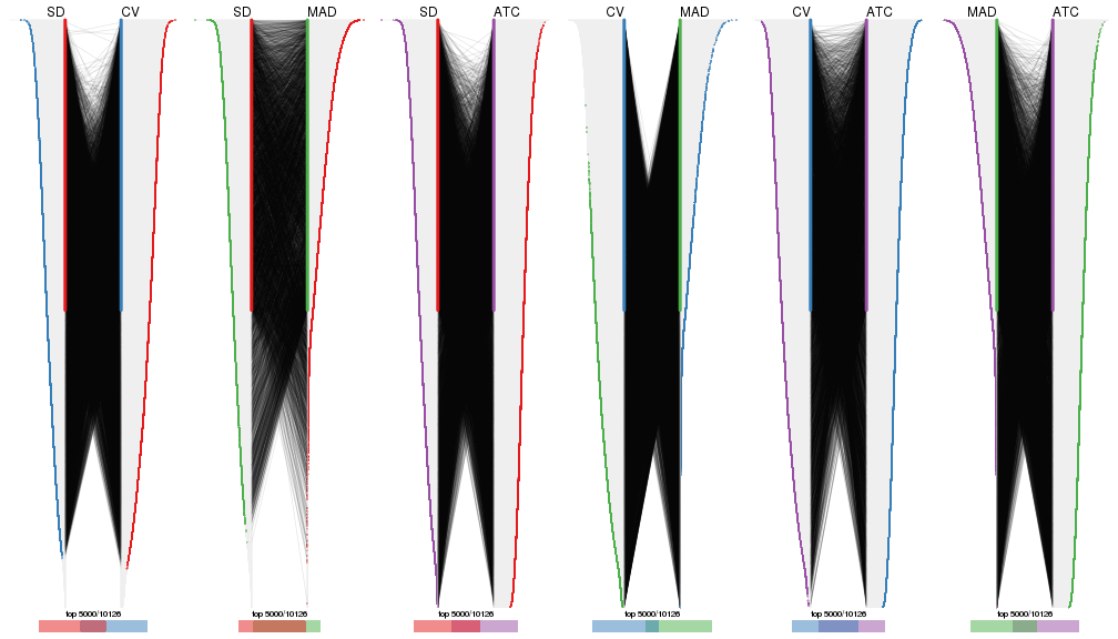
Overlap of top rows from different top-row methods:
top_rows_overlap(res_list, top_n = 1000, method = "euler")
top_rows_overlap(res_list, top_n = 2000, method = "euler")
top_rows_overlap(res_list, top_n = 3000, method = "euler")
top_rows_overlap(res_list, top_n = 4000, method = "euler")
top_rows_overlap(res_list, top_n = 5000, method = "euler")
Also visualize the correspondance of rankings between different top-row methods:
top_rows_overlap(res_list, top_n = 1000, method = "correspondance")
top_rows_overlap(res_list, top_n = 2000, method = "correspondance")
top_rows_overlap(res_list, top_n = 3000, method = "correspondance")
top_rows_overlap(res_list, top_n = 4000, method = "correspondance")
top_rows_overlap(res_list, top_n = 5000, method = "correspondance")
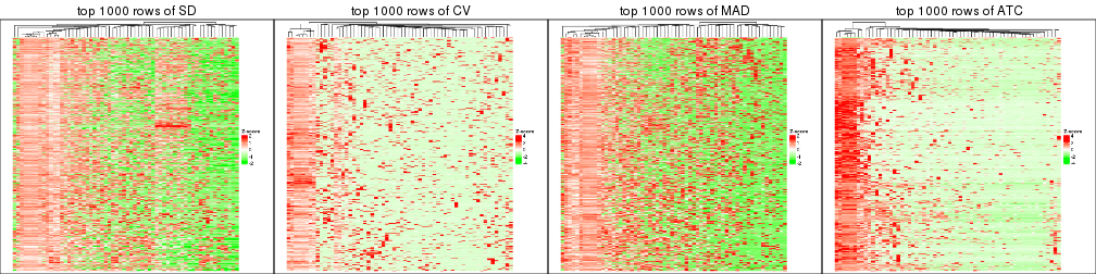
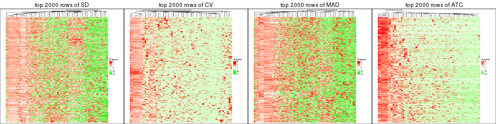
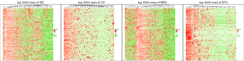
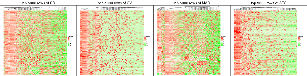
Heatmaps of the top rows:
top_rows_heatmap(res_list, top_n = 1000)
top_rows_heatmap(res_list, top_n = 2000)
top_rows_heatmap(res_list, top_n = 3000)
top_rows_heatmap(res_list, top_n = 4000)
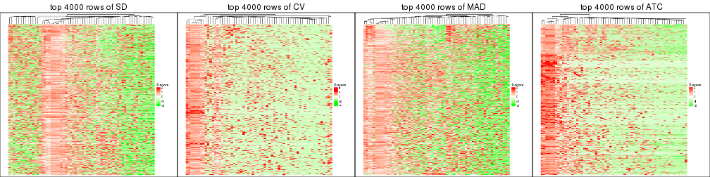
top_rows_heatmap(res_list, top_n = 5000)
The object with results only for a single top-value method and a single partition method can be extracted as:
res = res_list["SD", "hclust"]
# you can also extract it by
# res = res_list["SD:hclust"]
A summary of res and all the functions that can be applied to it:
res
#> A 'ConsensusPartition' object with k = 2, 3, 4, 5, 6.
#>   On a matrix with 10126 rows and 62 columns.
#>   Top rows (1000, 2000, 3000, 4000, 5000) are extracted by 'SD' method.
#>   Subgroups are detected by 'hclust' method.
#>   Performed in total 1250 partitions by row resampling.
#>   Best k for subgroups seems to be 2.
#>
#> Following methods can be applied to this 'ConsensusPartition' object:
#>  [1] "cola_report"             "collect_classes"         "collect_plots"
#>  [4] "collect_stats"           "colnames"                "compare_signatures"
#>  [7] "consensus_heatmap"       "dimension_reduction"     "functional_enrichment"
#> [10] "get_anno_col"            "get_anno"                "get_classes"
#> [13] "get_consensus"           "get_matrix"              "get_membership"
#> [16] "get_param"               "get_signatures"          "get_stats"
#> [19] "is_best_k"               "is_stable_k"             "membership_heatmap"
#> [22] "ncol"                    "nrow"                    "plot_ecdf"
#> [25] "rownames"                "select_partition_number" "show"
#> [28] "suggest_best_k"          "test_to_known_factors"
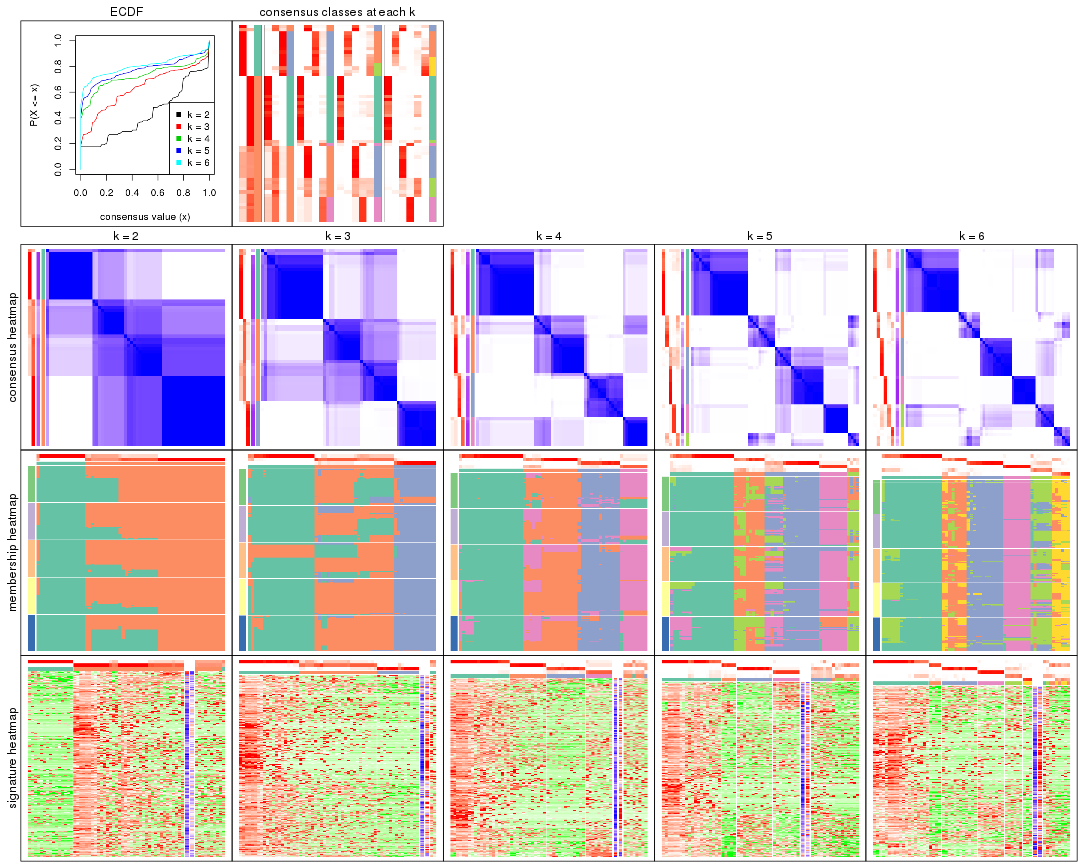
collect_plots() function collects all the plots made from res for all k (number of partitions)
into one single page to provide an easy and fast comparison between different k.
collect_plots(res)
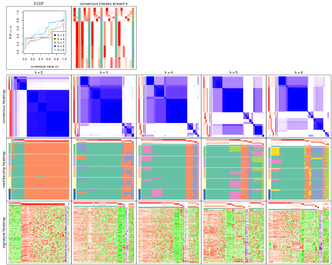
The plots are:
k and the heatmap of
predicted classes for each k.k.k.k.All the plots in panels can be made by individual functions and they are plotted later in this section.
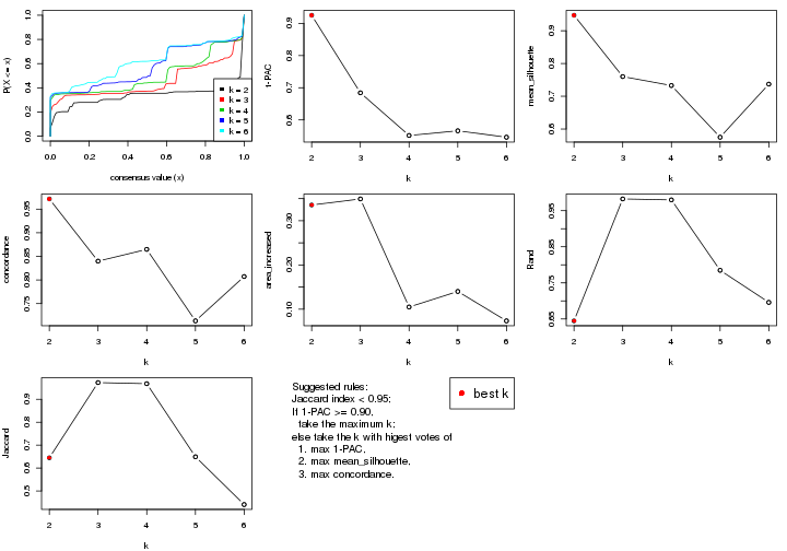
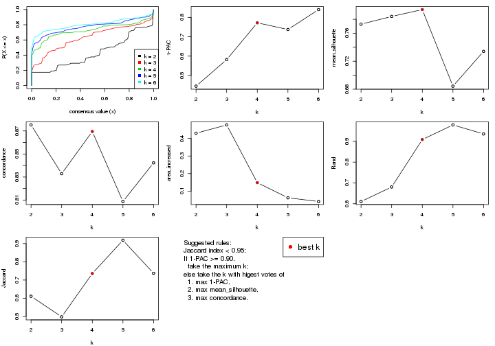
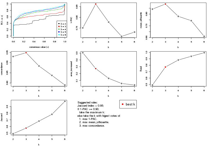
select_partition_number() produces several plots showing different
statistics for choosing “optimized” k. There are following statistics:
k;k, the area increased is defined as \(A_k - A_{k-1}\).The detailed explanations of these statistics can be found in the cola vignette.
Generally speaking, lower PAC score, higher mean silhouette score or higher
concordance corresponds to better partition. Rand index and Jaccard index
measure how similar the current partition is compared to partition with k-1.
If they are too similar, we won't accept k is better than k-1.
select_partition_number(res)
The numeric values for all these statistics can be obtained by get_stats().
get_stats(res)
#>   k 1-PAC mean_silhouette concordance area_increased  Rand Jaccard
#> 2 2 0.925           0.947       0.972         0.3355 0.645   0.645
#> 3 3 0.684           0.760       0.840         0.3493 0.983   0.973
#> 4 4 0.552           0.733       0.865         0.1050 0.980   0.968
#> 5 5 0.566           0.575       0.713         0.1402 0.785   0.649
#> 6 6 0.546           0.737       0.807         0.0736 0.696   0.441
suggest_best_k() suggests the best \(k\) based on these statistics. The rules are as follows:
suggest_best_k(res)
#> [1] 2
Following shows the table of the partitions (You need to click the show/hide
code output link to see it). The membership matrix (columns with name p*)
is inferred by
clue::cl_consensus()
function with the SE method. Basically the value in the membership matrix
represents the probability to belong to a certain group. The finall class
label for an item is determined with the group with highest probability it
belongs to.
In get_classes() function, the entropy is calculated from the membership
matrix and the silhouette score is calculated from the consensus matrix.
cbind(get_classes(res, k = 2), get_membership(res, k = 2))
#>            class entropy silhouette    p1    p2
#> SRR764776      2  0.0000      0.989 0.000 1.000
#> SRR764777      2  0.0000      0.989 0.000 1.000
#> SRR764778      2  0.0000      0.989 0.000 1.000
#> SRR764779      2  0.0000      0.989 0.000 1.000
#> SRR764780      2  0.0000      0.989 0.000 1.000
#> SRR764781      2  0.0000      0.989 0.000 1.000
#> SRR764782      2  0.0000      0.989 0.000 1.000
#> SRR764783      2  0.0000      0.989 0.000 1.000
#> SRR764784      2  0.0000      0.989 0.000 1.000
#> SRR764785      1  0.9661      0.455 0.608 0.392
#> SRR764786      1  0.9460      0.519 0.636 0.364
#> SRR764787      2  0.0000      0.989 0.000 1.000
#> SRR764788      2  0.0000      0.989 0.000 1.000
#> SRR764789      2  0.0000      0.989 0.000 1.000
#> SRR764790      1  0.0000      0.895 1.000 0.000
#> SRR764791      2  0.0000      0.989 0.000 1.000
#> SRR764792      2  0.0000      0.989 0.000 1.000
#> SRR764793      2  0.0000      0.989 0.000 1.000
#> SRR764794      2  0.2423      0.958 0.040 0.960
#> SRR764795      2  0.0000      0.989 0.000 1.000
#> SRR764796      2  0.0000      0.989 0.000 1.000
#> SRR764797      2  0.0000      0.989 0.000 1.000
#> SRR764798      2  0.1414      0.981 0.020 0.980
#> SRR764799      2  0.0000      0.989 0.000 1.000
#> SRR764800      2  0.0000      0.989 0.000 1.000
#> SRR764801      2  0.1414      0.981 0.020 0.980
#> SRR764802      2  0.0000      0.989 0.000 1.000
#> SRR764803      2  0.0000      0.989 0.000 1.000
#> SRR764804      1  0.0672      0.896 0.992 0.008
#> SRR764805      1  0.4690      0.867 0.900 0.100
#> SRR764806      2  0.1414      0.981 0.020 0.980
#> SRR764807      1  0.0000      0.895 1.000 0.000
#> SRR764808      1  0.0000      0.895 1.000 0.000
#> SRR764809      1  0.4690      0.867 0.900 0.100
#> SRR764810      1  0.4562      0.869 0.904 0.096
#> SRR764811      1  0.0000      0.895 1.000 0.000
#> SRR764812      1  0.0672      0.896 0.992 0.008
#> SRR764813      1  0.0672      0.896 0.992 0.008
#> SRR764814      2  0.0000      0.989 0.000 1.000
#> SRR764815      2  0.0000      0.989 0.000 1.000
#> SRR764816      2  0.0000      0.989 0.000 1.000
#> SRR764817      2  0.0000      0.989 0.000 1.000
#> SRR1066622     2  0.1184      0.982 0.016 0.984
#> SRR1066623     2  0.1184      0.982 0.016 0.984
#> SRR1066624     2  0.1184      0.982 0.016 0.984
#> SRR1066625     2  0.1184      0.982 0.016 0.984
#> SRR1066626     2  0.1184      0.982 0.016 0.984
#> SRR1066627     2  0.1184      0.982 0.016 0.984
#> SRR1066628     2  0.1184      0.982 0.016 0.984
#> SRR1066629     2  0.1184      0.982 0.016 0.984
#> SRR1066630     1  0.8016      0.718 0.756 0.244
#> SRR1066631     2  0.1184      0.982 0.016 0.984
#> SRR1066632     2  0.1414      0.981 0.020 0.980
#> SRR1066633     2  0.1414      0.981 0.020 0.980
#> SRR1066634     2  0.1184      0.983 0.016 0.984
#> SRR1066635     2  0.2603      0.959 0.044 0.956
#> SRR1066636     2  0.1414      0.981 0.020 0.980
#> SRR1066637     2  0.1414      0.981 0.020 0.980
#> SRR1066638     2  0.1414      0.981 0.020 0.980
#> SRR1066639     2  0.1414      0.981 0.020 0.980
#> SRR1066640     2  0.1414      0.981 0.020 0.980
#> SRR1066641     1  0.0000      0.895 1.000 0.000
cbind(get_classes(res, k = 3), get_membership(res, k = 3))
#>            class entropy silhouette    p1    p2    p3
#> SRR764776      1  0.0000      0.903 1.000 0.000 0.000
#> SRR764777      1  0.0000      0.903 1.000 0.000 0.000
#> SRR764778      1  0.0000      0.903 1.000 0.000 0.000
#> SRR764779      1  0.0000      0.903 1.000 0.000 0.000
#> SRR764780      1  0.0000      0.903 1.000 0.000 0.000
#> SRR764781      1  0.0000      0.903 1.000 0.000 0.000
#> SRR764782      1  0.0000      0.903 1.000 0.000 0.000
#> SRR764783      1  0.0000      0.903 1.000 0.000 0.000
#> SRR764784      1  0.0000      0.903 1.000 0.000 0.000
#> SRR764785      2  0.8046      0.314 0.068 0.536 0.396
#> SRR764786      2  0.7533      0.339 0.044 0.564 0.392
#> SRR764787      1  0.0237      0.902 0.996 0.000 0.004
#> SRR764788      1  0.0000      0.903 1.000 0.000 0.000
#> SRR764789      1  0.4002      0.808 0.840 0.000 0.160
#> SRR764790      2  0.0000      0.573 0.000 1.000 0.000
#> SRR764791      1  0.0237      0.902 0.996 0.000 0.004
#> SRR764792      1  0.0237      0.902 0.996 0.000 0.004
#> SRR764793      1  0.0000      0.903 1.000 0.000 0.000
#> SRR764794      1  0.4399      0.791 0.812 0.000 0.188
#> SRR764795      1  0.0000      0.903 1.000 0.000 0.000
#> SRR764796      1  0.0000      0.903 1.000 0.000 0.000
#> SRR764797      1  0.0000      0.903 1.000 0.000 0.000
#> SRR764798      1  0.2066      0.881 0.940 0.000 0.060
#> SRR764799      1  0.0000      0.903 1.000 0.000 0.000
#> SRR764800      1  0.0000      0.903 1.000 0.000 0.000
#> SRR764801      1  0.2066      0.881 0.940 0.000 0.060
#> SRR764802      1  0.0000      0.903 1.000 0.000 0.000
#> SRR764803      1  0.0000      0.903 1.000 0.000 0.000
#> SRR764804      2  0.5760     -0.251 0.000 0.672 0.328
#> SRR764805      3  0.6345      0.987 0.004 0.400 0.596
#> SRR764806      1  0.3038      0.851 0.896 0.000 0.104
#> SRR764807      2  0.0000      0.573 0.000 1.000 0.000
#> SRR764808      2  0.0000      0.573 0.000 1.000 0.000
#> SRR764809      3  0.6373      0.984 0.004 0.408 0.588
#> SRR764810      3  0.6359      0.987 0.004 0.404 0.592
#> SRR764811      2  0.1529      0.554 0.000 0.960 0.040
#> SRR764812      2  0.5733     -0.236 0.000 0.676 0.324
#> SRR764813      2  0.3619      0.417 0.000 0.864 0.136
#> SRR764814      1  0.0000      0.903 1.000 0.000 0.000
#> SRR764815      1  0.0592      0.901 0.988 0.000 0.012
#> SRR764816      1  0.0000      0.903 1.000 0.000 0.000
#> SRR764817      1  0.0000      0.903 1.000 0.000 0.000
#> SRR1066622     1  0.5905      0.631 0.648 0.000 0.352
#> SRR1066623     1  0.5905      0.631 0.648 0.000 0.352
#> SRR1066624     1  0.5905      0.631 0.648 0.000 0.352
#> SRR1066625     1  0.5905      0.631 0.648 0.000 0.352
#> SRR1066626     1  0.5905      0.631 0.648 0.000 0.352
#> SRR1066627     1  0.5905      0.631 0.648 0.000 0.352
#> SRR1066628     1  0.5905      0.631 0.648 0.000 0.352
#> SRR1066629     1  0.5905      0.631 0.648 0.000 0.352
#> SRR1066630     2  0.6168      0.429 0.036 0.740 0.224
#> SRR1066631     1  0.5905      0.631 0.648 0.000 0.352
#> SRR1066632     1  0.2066      0.881 0.940 0.000 0.060
#> SRR1066633     1  0.2066      0.881 0.940 0.000 0.060
#> SRR1066634     1  0.1860      0.884 0.948 0.000 0.052
#> SRR1066635     1  0.3845      0.833 0.872 0.012 0.116
#> SRR1066636     1  0.2066      0.881 0.940 0.000 0.060
#> SRR1066637     1  0.2066      0.881 0.940 0.000 0.060
#> SRR1066638     1  0.2537      0.868 0.920 0.000 0.080
#> SRR1066639     1  0.2066      0.881 0.940 0.000 0.060
#> SRR1066640     1  0.2066      0.881 0.940 0.000 0.060
#> SRR1066641     2  0.1529      0.554 0.000 0.960 0.040
cbind(get_classes(res, k = 4), get_membership(res, k = 4))
#>            class entropy silhouette    p1    p2    p3    p4
#> SRR764776      1  0.0000      0.852 1.000 0.000 0.000 0.000
#> SRR764777      1  0.0000      0.852 1.000 0.000 0.000 0.000
#> SRR764778      1  0.0000      0.852 1.000 0.000 0.000 0.000
#> SRR764779      1  0.0000      0.852 1.000 0.000 0.000 0.000
#> SRR764780      1  0.0000      0.852 1.000 0.000 0.000 0.000
#> SRR764781      1  0.0000      0.852 1.000 0.000 0.000 0.000
#> SRR764782      1  0.0000      0.852 1.000 0.000 0.000 0.000
#> SRR764783      1  0.0000      0.852 1.000 0.000 0.000 0.000
#> SRR764784      1  0.0000      0.852 1.000 0.000 0.000 0.000
#> SRR764785      4  0.4377      0.945 0.008 0.188 0.016 0.788
#> SRR764786      4  0.4399      0.943 0.000 0.224 0.016 0.760
#> SRR764787      1  0.0188      0.850 0.996 0.000 0.000 0.004
#> SRR764788      1  0.0000      0.852 1.000 0.000 0.000 0.000
#> SRR764789      1  0.3583      0.726 0.816 0.000 0.004 0.180
#> SRR764790      2  0.0921      0.845 0.000 0.972 0.000 0.028
#> SRR764791      1  0.0188      0.850 0.996 0.000 0.000 0.004
#> SRR764792      1  0.0188      0.850 0.996 0.000 0.000 0.004
#> SRR764793      1  0.0000      0.852 1.000 0.000 0.000 0.000
#> SRR764794      1  0.3688      0.707 0.792 0.000 0.000 0.208
#> SRR764795      1  0.0000      0.852 1.000 0.000 0.000 0.000
#> SRR764796      1  0.0000      0.852 1.000 0.000 0.000 0.000
#> SRR764797      1  0.0000      0.852 1.000 0.000 0.000 0.000
#> SRR764798      1  0.3448      0.772 0.828 0.000 0.004 0.168
#> SRR764799      1  0.0000      0.852 1.000 0.000 0.000 0.000
#> SRR764800      1  0.0000      0.852 1.000 0.000 0.000 0.000
#> SRR764801      1  0.3448      0.772 0.828 0.000 0.004 0.168
#> SRR764802      1  0.0000      0.852 1.000 0.000 0.000 0.000
#> SRR764803      1  0.0000      0.852 1.000 0.000 0.000 0.000
#> SRR764804      3  0.5000      0.262 0.000 0.496 0.504 0.000
#> SRR764805      3  0.0927      0.693 0.000 0.016 0.976 0.008
#> SRR764806      1  0.4669      0.742 0.780 0.000 0.052 0.168
#> SRR764807      2  0.0921      0.845 0.000 0.972 0.000 0.028
#> SRR764808      2  0.0921      0.845 0.000 0.972 0.000 0.028
#> SRR764809      3  0.1256      0.696 0.000 0.028 0.964 0.008
#> SRR764810      3  0.0895      0.692 0.000 0.020 0.976 0.004
#> SRR764811      2  0.1837      0.826 0.000 0.944 0.028 0.028
#> SRR764812      3  0.5000      0.251 0.000 0.500 0.500 0.000
#> SRR764813      2  0.3450      0.678 0.000 0.836 0.156 0.008
#> SRR764814      1  0.0000      0.852 1.000 0.000 0.000 0.000
#> SRR764815      1  0.0469      0.849 0.988 0.000 0.000 0.012
#> SRR764816      1  0.0000      0.852 1.000 0.000 0.000 0.000
#> SRR764817      1  0.0000      0.852 1.000 0.000 0.000 0.000
#> SRR1066622     1  0.4843      0.447 0.604 0.000 0.000 0.396
#> SRR1066623     1  0.4843      0.447 0.604 0.000 0.000 0.396
#> SRR1066624     1  0.4843      0.447 0.604 0.000 0.000 0.396
#> SRR1066625     1  0.4843      0.447 0.604 0.000 0.000 0.396
#> SRR1066626     1  0.4843      0.447 0.604 0.000 0.000 0.396
#> SRR1066627     1  0.4843      0.447 0.604 0.000 0.000 0.396
#> SRR1066628     1  0.4843      0.447 0.604 0.000 0.000 0.396
#> SRR1066629     1  0.4843      0.447 0.604 0.000 0.000 0.396
#> SRR1066630     2  0.4585      0.149 0.000 0.668 0.000 0.332
#> SRR1066631     1  0.4843      0.447 0.604 0.000 0.000 0.396
#> SRR1066632     1  0.3402      0.775 0.832 0.000 0.004 0.164
#> SRR1066633     1  0.3448      0.772 0.828 0.000 0.004 0.168
#> SRR1066634     1  0.3257      0.782 0.844 0.000 0.004 0.152
#> SRR1066635     1  0.5100      0.720 0.756 0.000 0.076 0.168
#> SRR1066636     1  0.3448      0.772 0.828 0.000 0.004 0.168
#> SRR1066637     1  0.3448      0.772 0.828 0.000 0.004 0.168
#> SRR1066638     1  0.4050      0.760 0.808 0.000 0.024 0.168
#> SRR1066639     1  0.3448      0.772 0.828 0.000 0.004 0.168
#> SRR1066640     1  0.3448      0.772 0.828 0.000 0.004 0.168
#> SRR1066641     2  0.1837      0.826 0.000 0.944 0.028 0.028
cbind(get_classes(res, k = 5), get_membership(res, k = 5))
#>            class entropy silhouette    p1    p2    p3    p4    p5
#> SRR764776      1  0.4297      0.547 0.528 0.000 0.000 0.472 0.000
#> SRR764777      1  0.4297      0.547 0.528 0.000 0.000 0.472 0.000
#> SRR764778      1  0.4297      0.547 0.528 0.000 0.000 0.472 0.000
#> SRR764779      1  0.4297      0.547 0.528 0.000 0.000 0.472 0.000
#> SRR764780      1  0.4297      0.547 0.528 0.000 0.000 0.472 0.000
#> SRR764781      1  0.4297      0.547 0.528 0.000 0.000 0.472 0.000
#> SRR764782      1  0.4297      0.547 0.528 0.000 0.000 0.472 0.000
#> SRR764783      1  0.4297      0.547 0.528 0.000 0.000 0.472 0.000
#> SRR764784      1  0.4297      0.547 0.528 0.000 0.000 0.472 0.000
#> SRR764785      5  0.3630      0.961 0.000 0.016 0.000 0.204 0.780
#> SRR764786      5  0.4201      0.961 0.000 0.044 0.000 0.204 0.752
#> SRR764787      1  0.4300      0.536 0.524 0.000 0.000 0.476 0.000
#> SRR764788      1  0.4297      0.547 0.528 0.000 0.000 0.472 0.000
#> SRR764789      4  0.5128      0.293 0.344 0.000 0.000 0.604 0.052
#> SRR764790      2  0.0451      0.777 0.000 0.988 0.000 0.004 0.008
#> SRR764791      1  0.4300      0.536 0.524 0.000 0.000 0.476 0.000
#> SRR764792      1  0.4300      0.536 0.524 0.000 0.000 0.476 0.000
#> SRR764793      1  0.4297      0.547 0.528 0.000 0.000 0.472 0.000
#> SRR764794      4  0.5422      0.318 0.348 0.000 0.000 0.580 0.072
#> SRR764795      1  0.4297      0.547 0.528 0.000 0.000 0.472 0.000
#> SRR764796      1  0.4297      0.547 0.528 0.000 0.000 0.472 0.000
#> SRR764797      1  0.4297      0.547 0.528 0.000 0.000 0.472 0.000
#> SRR764798      1  0.0162      0.375 0.996 0.000 0.000 0.000 0.004
#> SRR764799      1  0.4297      0.547 0.528 0.000 0.000 0.472 0.000
#> SRR764800      1  0.4297      0.547 0.528 0.000 0.000 0.472 0.000
#> SRR764801      1  0.0162      0.375 0.996 0.000 0.000 0.000 0.004
#> SRR764802      1  0.4297      0.547 0.528 0.000 0.000 0.472 0.000
#> SRR764803      1  0.4297      0.547 0.528 0.000 0.000 0.472 0.000
#> SRR764804      3  0.5770      0.252 0.000 0.456 0.480 0.040 0.024
#> SRR764805      3  0.0566      0.644 0.012 0.000 0.984 0.004 0.000
#> SRR764806      1  0.1630      0.326 0.944 0.000 0.036 0.004 0.016
#> SRR764807      2  0.0404      0.777 0.000 0.988 0.000 0.000 0.012
#> SRR764808      2  0.0324      0.778 0.000 0.992 0.000 0.004 0.004
#> SRR764809      3  0.1383      0.644 0.012 0.008 0.960 0.008 0.012
#> SRR764810      3  0.2889      0.619 0.000 0.000 0.872 0.044 0.084
#> SRR764811      2  0.4463      0.722 0.000 0.788 0.024 0.112 0.076
#> SRR764812      3  0.5771      0.242 0.000 0.460 0.476 0.040 0.024
#> SRR764813      2  0.5130      0.607 0.000 0.748 0.124 0.076 0.052
#> SRR764814      1  0.4297      0.547 0.528 0.000 0.000 0.472 0.000
#> SRR764815      1  0.4415      0.502 0.552 0.000 0.000 0.444 0.004
#> SRR764816      1  0.4297      0.547 0.528 0.000 0.000 0.472 0.000
#> SRR764817      1  0.4297      0.547 0.528 0.000 0.000 0.472 0.000
#> SRR1066622     4  0.4732      0.902 0.208 0.000 0.000 0.716 0.076
#> SRR1066623     4  0.4732      0.902 0.208 0.000 0.000 0.716 0.076
#> SRR1066624     4  0.4732      0.902 0.208 0.000 0.000 0.716 0.076
#> SRR1066625     4  0.4732      0.902 0.208 0.000 0.000 0.716 0.076
#> SRR1066626     4  0.4732      0.902 0.208 0.000 0.000 0.716 0.076
#> SRR1066627     4  0.4732      0.902 0.208 0.000 0.000 0.716 0.076
#> SRR1066628     4  0.4732      0.902 0.208 0.000 0.000 0.716 0.076
#> SRR1066629     4  0.4732      0.902 0.208 0.000 0.000 0.716 0.076
#> SRR1066630     2  0.5904      0.246 0.000 0.600 0.000 0.204 0.196
#> SRR1066631     4  0.4732      0.902 0.208 0.000 0.000 0.716 0.076
#> SRR1066632     1  0.0671      0.378 0.980 0.000 0.000 0.016 0.004
#> SRR1066633     1  0.0162      0.375 0.996 0.000 0.000 0.000 0.004
#> SRR1066634     1  0.1121      0.377 0.956 0.000 0.000 0.044 0.000
#> SRR1066635     1  0.2074      0.303 0.920 0.000 0.060 0.004 0.016
#> SRR1066636     1  0.0162      0.375 0.996 0.000 0.000 0.000 0.004
#> SRR1066637     1  0.0324      0.376 0.992 0.000 0.000 0.004 0.004
#> SRR1066638     1  0.0960      0.354 0.972 0.000 0.008 0.004 0.016
#> SRR1066639     1  0.0451      0.375 0.988 0.000 0.000 0.004 0.008
#> SRR1066640     1  0.0451      0.376 0.988 0.000 0.000 0.008 0.004
#> SRR1066641     2  0.4463      0.722 0.000 0.788 0.024 0.112 0.076
cbind(get_classes(res, k = 6), get_membership(res, k = 6))
#>            class entropy silhouette    p1    p2    p3    p4    p5    p6
#> SRR764776      1  0.0000      0.832 1.000 0.000 0.000 0.000 0.000 0.000
#> SRR764777      1  0.0000      0.832 1.000 0.000 0.000 0.000 0.000 0.000
#> SRR764778      1  0.0000      0.832 1.000 0.000 0.000 0.000 0.000 0.000
#> SRR764779      1  0.0000      0.832 1.000 0.000 0.000 0.000 0.000 0.000
#> SRR764780      1  0.0000      0.832 1.000 0.000 0.000 0.000 0.000 0.000
#> SRR764781      1  0.0000      0.832 1.000 0.000 0.000 0.000 0.000 0.000
#> SRR764782      1  0.0000      0.832 1.000 0.000 0.000 0.000 0.000 0.000
#> SRR764783      1  0.0000      0.832 1.000 0.000 0.000 0.000 0.000 0.000
#> SRR764784      1  0.0000      0.832 1.000 0.000 0.000 0.000 0.000 0.000
#> SRR764785      4  0.0000      0.961 0.000 0.000 0.000 1.000 0.000 0.000
#> SRR764786      4  0.1245      0.961 0.000 0.016 0.000 0.952 0.000 0.032
#> SRR764787      1  0.0146      0.831 0.996 0.000 0.000 0.004 0.000 0.000
#> SRR764788      1  0.0000      0.832 1.000 0.000 0.000 0.000 0.000 0.000
#> SRR764789      1  0.2730      0.705 0.808 0.000 0.000 0.192 0.000 0.000
#> SRR764790      2  0.0405      0.636 0.000 0.988 0.000 0.004 0.000 0.008
#> SRR764791      1  0.0146      0.831 0.996 0.000 0.000 0.004 0.000 0.000
#> SRR764792      1  0.0146      0.831 0.996 0.000 0.000 0.004 0.000 0.000
#> SRR764793      1  0.0000      0.832 1.000 0.000 0.000 0.000 0.000 0.000
#> SRR764794      1  0.3134      0.687 0.784 0.000 0.004 0.208 0.000 0.004
#> SRR764795      1  0.0000      0.832 1.000 0.000 0.000 0.000 0.000 0.000
#> SRR764796      1  0.0000      0.832 1.000 0.000 0.000 0.000 0.000 0.000
#> SRR764797      1  0.0000      0.832 1.000 0.000 0.000 0.000 0.000 0.000
#> SRR764798      3  0.3592      0.948 0.344 0.000 0.656 0.000 0.000 0.000
#> SRR764799      1  0.0000      0.832 1.000 0.000 0.000 0.000 0.000 0.000
#> SRR764800      1  0.0000      0.832 1.000 0.000 0.000 0.000 0.000 0.000
#> SRR764801      3  0.3592      0.948 0.344 0.000 0.656 0.000 0.000 0.000
#> SRR764802      1  0.0000      0.832 1.000 0.000 0.000 0.000 0.000 0.000
#> SRR764803      1  0.0000      0.832 1.000 0.000 0.000 0.000 0.000 0.000
#> SRR764804      5  0.5828      0.277 0.000 0.408 0.032 0.000 0.472 0.088
#> SRR764805      5  0.1151      0.595 0.000 0.000 0.032 0.000 0.956 0.012
#> SRR764806      3  0.3221      0.876 0.264 0.000 0.736 0.000 0.000 0.000
#> SRR764807      2  0.0806      0.636 0.000 0.972 0.000 0.008 0.000 0.020
#> SRR764808      2  0.0000      0.636 0.000 1.000 0.000 0.000 0.000 0.000
#> SRR764809      5  0.1606      0.592 0.000 0.000 0.056 0.004 0.932 0.008
#> SRR764810      5  0.4643      0.491 0.000 0.000 0.184 0.000 0.688 0.128
#> SRR764811      2  0.3991      0.484 0.000 0.524 0.000 0.000 0.004 0.472
#> SRR764812      5  0.5831      0.270 0.000 0.412 0.032 0.000 0.468 0.088
#> SRR764813      2  0.5933      0.418 0.000 0.616 0.068 0.008 0.084 0.224
#> SRR764814      1  0.0000      0.832 1.000 0.000 0.000 0.000 0.000 0.000
#> SRR764815      1  0.1462      0.760 0.936 0.000 0.056 0.008 0.000 0.000
#> SRR764816      1  0.0000      0.832 1.000 0.000 0.000 0.000 0.000 0.000
#> SRR764817      1  0.0000      0.832 1.000 0.000 0.000 0.000 0.000 0.000
#> SRR1066622     1  0.5276      0.554 0.604 0.000 0.000 0.188 0.000 0.208
#> SRR1066623     1  0.5276      0.554 0.604 0.000 0.000 0.188 0.000 0.208
#> SRR1066624     1  0.5276      0.554 0.604 0.000 0.000 0.188 0.000 0.208
#> SRR1066625     1  0.5276      0.554 0.604 0.000 0.000 0.188 0.000 0.208
#> SRR1066626     1  0.5276      0.554 0.604 0.000 0.000 0.188 0.000 0.208
#> SRR1066627     1  0.5276      0.554 0.604 0.000 0.000 0.188 0.000 0.208
#> SRR1066628     1  0.5276      0.554 0.604 0.000 0.000 0.188 0.000 0.208
#> SRR1066629     1  0.5276      0.554 0.604 0.000 0.000 0.188 0.000 0.208
#> SRR1066630     2  0.5829      0.117 0.000 0.516 0.028 0.104 0.000 0.352
#> SRR1066631     1  0.5276      0.554 0.604 0.000 0.000 0.188 0.000 0.208
#> SRR1066632     3  0.3695      0.920 0.376 0.000 0.624 0.000 0.000 0.000
#> SRR1066633     3  0.3578      0.947 0.340 0.000 0.660 0.000 0.000 0.000
#> SRR1066634     3  0.3804      0.846 0.424 0.000 0.576 0.000 0.000 0.000
#> SRR1066635     3  0.3665      0.852 0.252 0.000 0.728 0.000 0.020 0.000
#> SRR1066636     3  0.3578      0.947 0.340 0.000 0.660 0.000 0.000 0.000
#> SRR1066637     3  0.3607      0.946 0.348 0.000 0.652 0.000 0.000 0.000
#> SRR1066638     3  0.3371      0.909 0.292 0.000 0.708 0.000 0.000 0.000
#> SRR1066639     3  0.3592      0.947 0.344 0.000 0.656 0.000 0.000 0.000
#> SRR1066640     3  0.3634      0.940 0.356 0.000 0.644 0.000 0.000 0.000
#> SRR1066641     2  0.3991      0.484 0.000 0.524 0.000 0.000 0.004 0.472
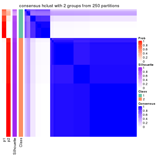
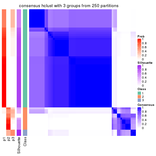
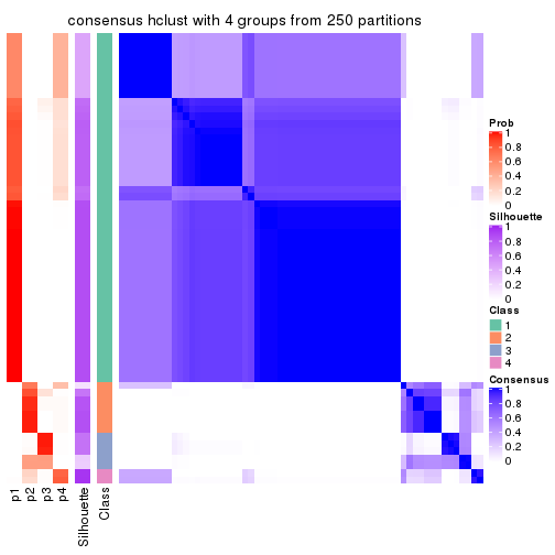
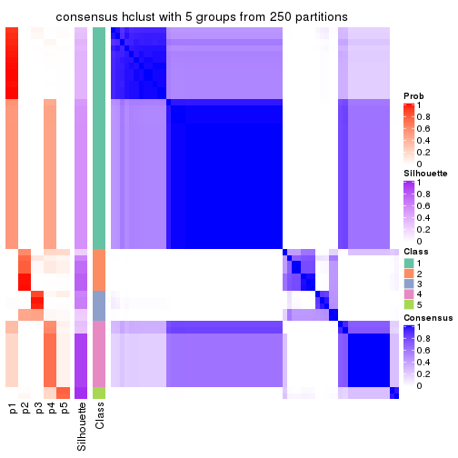
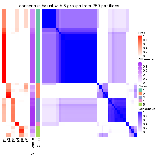
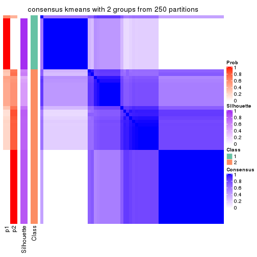
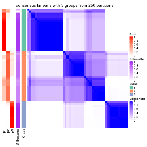
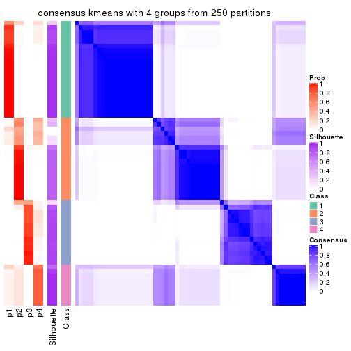
Heatmaps for the consensus matrix. It visualizes the probability of two samples to be in a same group.
consensus_heatmap(res, k = 2)
consensus_heatmap(res, k = 3)
consensus_heatmap(res, k = 4)
consensus_heatmap(res, k = 5)
consensus_heatmap(res, k = 6)
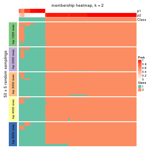
Heatmaps for the membership of samples in all partitions to see how consistent they are:
membership_heatmap(res, k = 2)
membership_heatmap(res, k = 3)
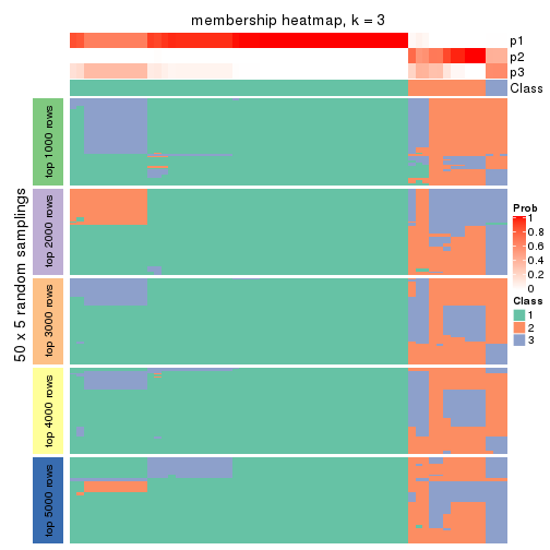
membership_heatmap(res, k = 4)
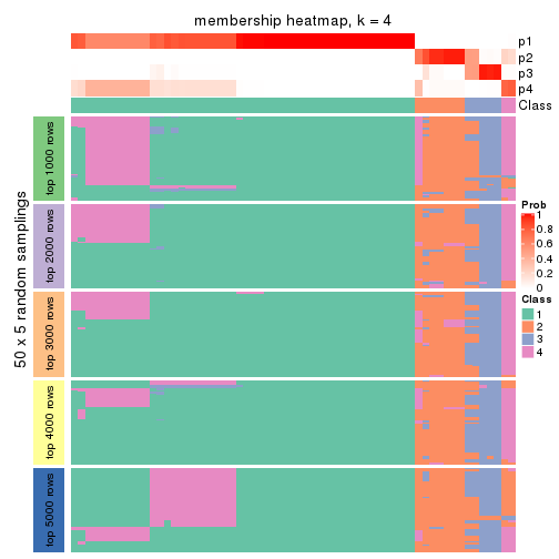
membership_heatmap(res, k = 5)
membership_heatmap(res, k = 6)
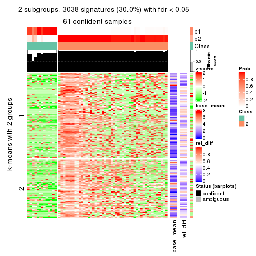
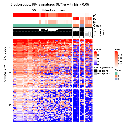
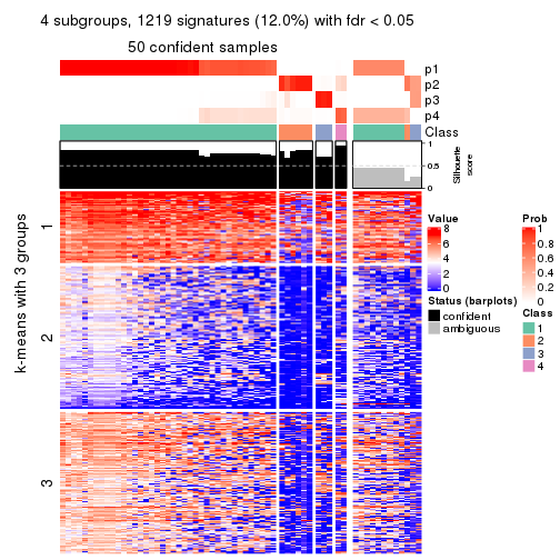
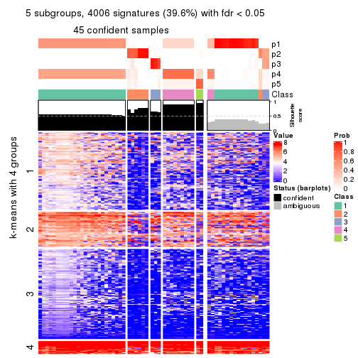
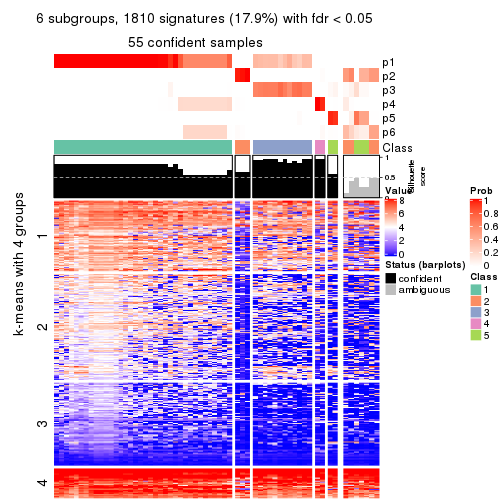
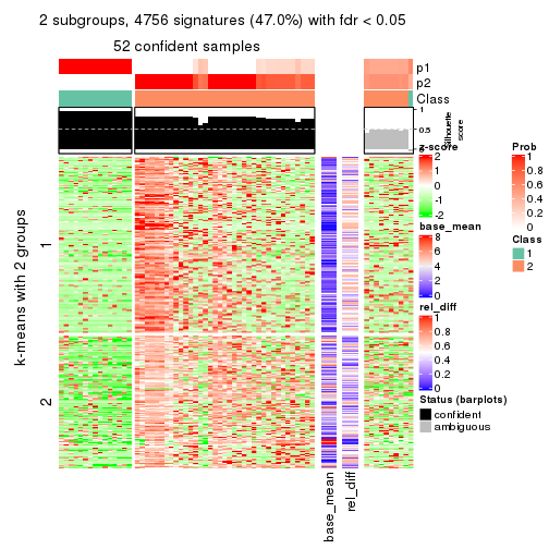
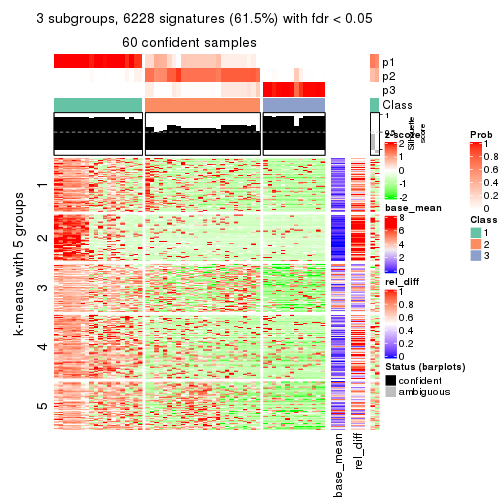
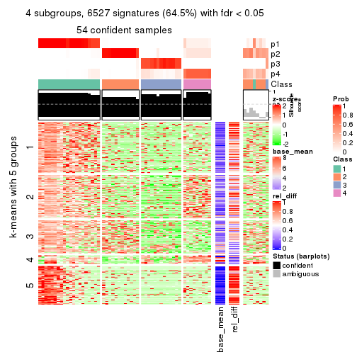
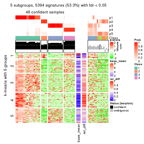
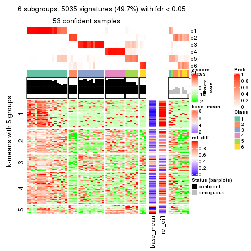
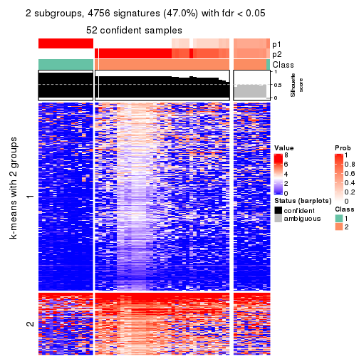
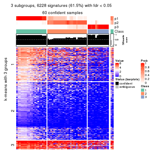
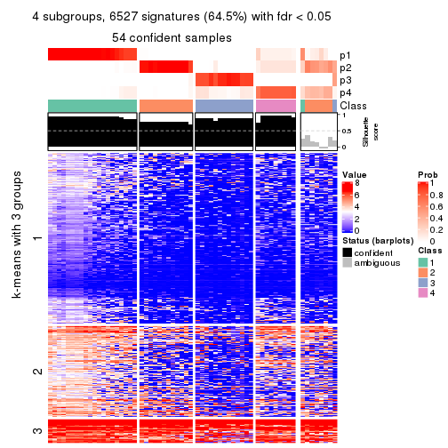
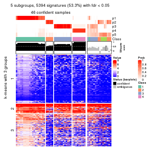
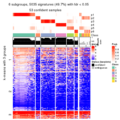
As soon as we have had the classes for columns, we can look for signatures which are significantly different between classes which can be candidate marks for certain classes. Following are the heatmaps for signatures.
Signature heatmaps where rows are scaled:
get_signatures(res, k = 2)
get_signatures(res, k = 3)
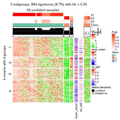
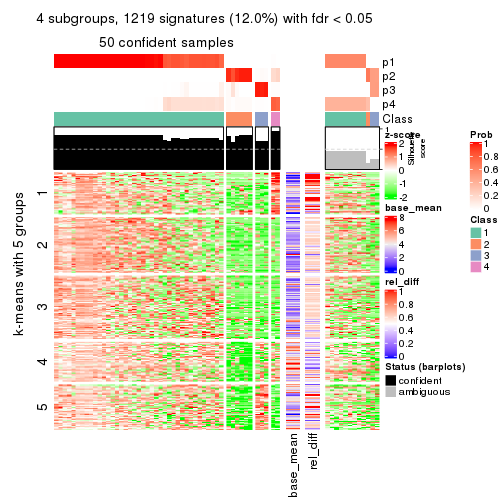
get_signatures(res, k = 4)
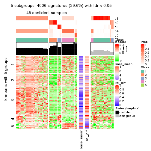
get_signatures(res, k = 5)
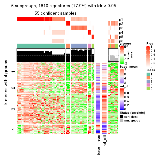
get_signatures(res, k = 6)
Signature heatmaps where rows are not scaled:
get_signatures(res, k = 2, scale_rows = FALSE)
get_signatures(res, k = 3, scale_rows = FALSE)
get_signatures(res, k = 4, scale_rows = FALSE)
get_signatures(res, k = 5, scale_rows = FALSE)
get_signatures(res, k = 6, scale_rows = FALSE)
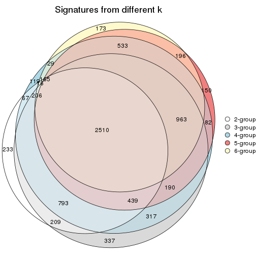
Compare the overlap of signatures from different k:
compare_signatures(res)
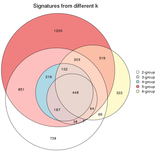
get_signature() returns a data frame invisibly. TO get the list of signatures, the function
call should be assigned to a variable explicitly. In following code, if plot argument is set
to FALSE, no heatmap is plotted while only the differential analysis is performed.
# code only for demonstration
tb = get_signature(res, k = ..., plot = FALSE)
An example of the output of tb is:
#>   which_row         fdr    mean_1    mean_2 scaled_mean_1 scaled_mean_2 km
#> 1        38 0.042760348  8.373488  9.131774    -0.5533452     0.5164555  1
#> 2        40 0.018707592  7.106213  8.469186    -0.6173731     0.5762149  1
#> 3        55 0.019134737 10.221463 11.207825    -0.6159697     0.5749050  1
#> 4        59 0.006059896  5.921854  7.869574    -0.6899429     0.6439467  1
#> 5        60 0.018055526  8.928898 10.211722    -0.6204761     0.5791110  1
#> 6        98 0.009384629 15.714769 14.887706     0.6635654    -0.6193277  2
...
The columns in tb are:
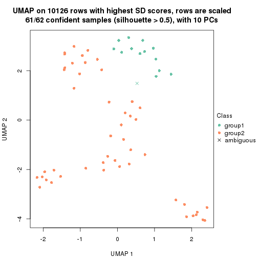
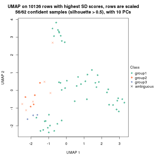
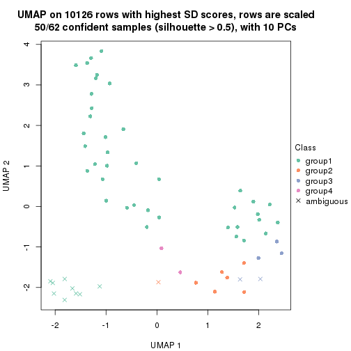
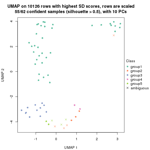
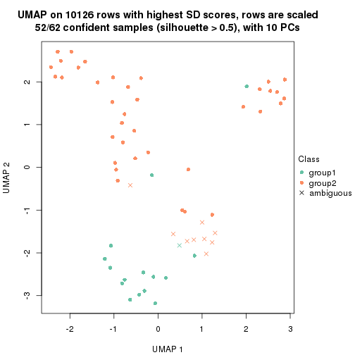
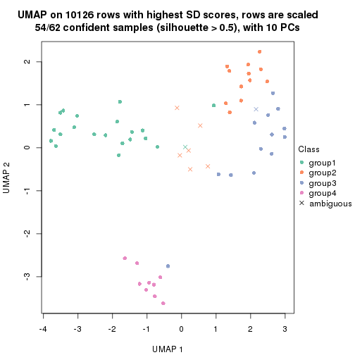
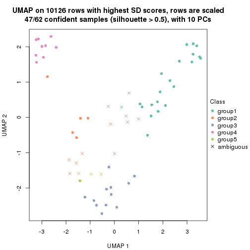
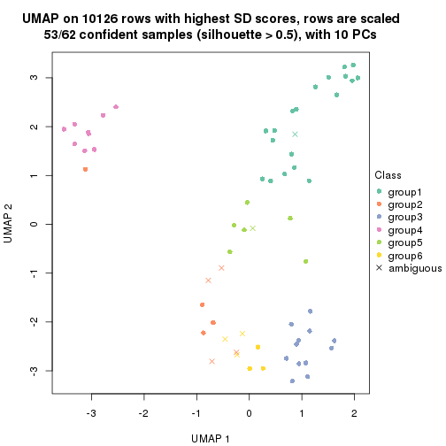
which_row: row indices corresponding to the input matrix.fdr: FDR for the differential test. mean_x: The mean value in group x.scaled_mean_x: The mean value in group x after rows are scaled.km: Row groups if k-means clustering is applied to rows.UMAP plot which shows how samples are separated.
dimension_reduction(res, k = 2, method = "UMAP")
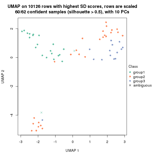
dimension_reduction(res, k = 3, method = "UMAP")
dimension_reduction(res, k = 4, method = "UMAP")
dimension_reduction(res, k = 5, method = "UMAP")
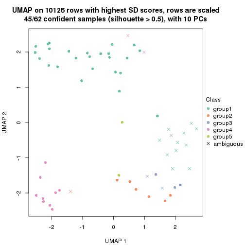
dimension_reduction(res, k = 6, method = "UMAP")
Following heatmap shows how subgroups are split when increasing k:
collect_classes(res)
If matrix rows can be associated to genes, consider to use functional_enrichment(res,
...) to perform function enrichment for the signature genes. See this vignette for more detailed explanations.
The object with results only for a single top-value method and a single partition method can be extracted as:
res = res_list["SD", "kmeans"]
# you can also extract it by
# res = res_list["SD:kmeans"]
A summary of res and all the functions that can be applied to it:
res
#> A 'ConsensusPartition' object with k = 2, 3, 4, 5, 6.
#>   On a matrix with 10126 rows and 62 columns.
#>   Top rows (1000, 2000, 3000, 4000, 5000) are extracted by 'SD' method.
#>   Subgroups are detected by 'kmeans' method.
#>   Performed in total 1250 partitions by row resampling.
#>   Best k for subgroups seems to be 4.
#>
#> Following methods can be applied to this 'ConsensusPartition' object:
#>  [1] "cola_report"             "collect_classes"         "collect_plots"
#>  [4] "collect_stats"           "colnames"                "compare_signatures"
#>  [7] "consensus_heatmap"       "dimension_reduction"     "functional_enrichment"
#> [10] "get_anno_col"            "get_anno"                "get_classes"
#> [13] "get_consensus"           "get_matrix"              "get_membership"
#> [16] "get_param"               "get_signatures"          "get_stats"
#> [19] "is_best_k"               "is_stable_k"             "membership_heatmap"
#> [22] "ncol"                    "nrow"                    "plot_ecdf"
#> [25] "rownames"                "select_partition_number" "show"
#> [28] "suggest_best_k"          "test_to_known_factors"
collect_plots() function collects all the plots made from res for all k (number of partitions)
into one single page to provide an easy and fast comparison between different k.
collect_plots(res)
The plots are:
k and the heatmap of
predicted classes for each k.k.k.k.All the plots in panels can be made by individual functions and they are plotted later in this section.
select_partition_number() produces several plots showing different
statistics for choosing “optimized” k. There are following statistics:
k;k, the area increased is defined as \(A_k - A_{k-1}\).The detailed explanations of these statistics can be found in the cola vignette.
Generally speaking, lower PAC score, higher mean silhouette score or higher
concordance corresponds to better partition. Rand index and Jaccard index
measure how similar the current partition is compared to partition with k-1.
If they are too similar, we won't accept k is better than k-1.
select_partition_number(res)
The numeric values for all these statistics can be obtained by get_stats().
get_stats(res)
#>   k 1-PAC mean_silhouette concordance area_increased  Rand Jaccard
#> 2 2 0.445           0.773       0.875         0.4298 0.611   0.611
#> 3 3 0.582           0.784       0.833         0.4771 0.681   0.498
#> 4 4 0.772           0.794       0.870         0.1481 0.909   0.736
#> 5 5 0.737           0.684       0.809         0.0618 0.979   0.918
#> 6 6 0.840           0.734       0.842         0.0407 0.935   0.737
suggest_best_k() suggests the best \(k\) based on these statistics. The rules are as follows:
suggest_best_k(res)
#> [1] 4
Following shows the table of the partitions (You need to click the show/hide
code output link to see it). The membership matrix (columns with name p*)
is inferred by
clue::cl_consensus()
function with the SE method. Basically the value in the membership matrix
represents the probability to belong to a certain group. The finall class
label for an item is determined with the group with highest probability it
belongs to.
In get_classes() function, the entropy is calculated from the membership
matrix and the silhouette score is calculated from the consensus matrix.
cbind(get_classes(res, k = 2), get_membership(res, k = 2))
#>            class entropy silhouette    p1    p2
#> SRR764776      2   0.000     0.8157 0.000 1.000
#> SRR764777      2   0.000     0.8157 0.000 1.000
#> SRR764778      2   0.000     0.8157 0.000 1.000
#> SRR764779      2   0.000     0.8157 0.000 1.000
#> SRR764780      2   0.000     0.8157 0.000 1.000
#> SRR764781      2   0.000     0.8157 0.000 1.000
#> SRR764782      2   0.000     0.8157 0.000 1.000
#> SRR764783      2   0.000     0.8157 0.000 1.000
#> SRR764784      2   0.000     0.8157 0.000 1.000
#> SRR764785      1   0.000     0.9635 1.000 0.000
#> SRR764786      1   0.000     0.9635 1.000 0.000
#> SRR764787      2   0.697     0.7793 0.188 0.812
#> SRR764788      2   0.000     0.8157 0.000 1.000
#> SRR764789      2   0.738     0.7716 0.208 0.792
#> SRR764790      1   0.000     0.9635 1.000 0.000
#> SRR764791      2   0.730     0.7733 0.204 0.796
#> SRR764792      2   0.634     0.7874 0.160 0.840
#> SRR764793      2   0.000     0.8157 0.000 1.000
#> SRR764794      2   0.999     0.4140 0.480 0.520
#> SRR764795      2   0.000     0.8157 0.000 1.000
#> SRR764796      2   0.000     0.8157 0.000 1.000
#> SRR764797      2   0.000     0.8157 0.000 1.000
#> SRR764798      2   0.904     0.6104 0.320 0.680
#> SRR764799      2   0.000     0.8157 0.000 1.000
#> SRR764800      2   0.000     0.8157 0.000 1.000
#> SRR764801      2   0.861     0.6447 0.284 0.716
#> SRR764802      2   0.000     0.8157 0.000 1.000
#> SRR764803      2   0.000     0.8157 0.000 1.000
#> SRR764804      1   0.000     0.9635 1.000 0.000
#> SRR764805      1   0.000     0.9635 1.000 0.000
#> SRR764806      2   0.991     0.4960 0.444 0.556
#> SRR764807      1   0.000     0.9635 1.000 0.000
#> SRR764808      1   0.000     0.9635 1.000 0.000
#> SRR764809      1   0.000     0.9635 1.000 0.000
#> SRR764810      1   0.000     0.9635 1.000 0.000
#> SRR764811      1   0.000     0.9635 1.000 0.000
#> SRR764812      1   0.000     0.9635 1.000 0.000
#> SRR764813      1   0.000     0.9635 1.000 0.000
#> SRR764814      2   0.000     0.8157 0.000 1.000
#> SRR764815      2   0.738     0.7716 0.208 0.792
#> SRR764816      2   0.000     0.8157 0.000 1.000
#> SRR764817      2   0.000     0.8157 0.000 1.000
#> SRR1066622     2   0.738     0.7716 0.208 0.792
#> SRR1066623     2   0.738     0.7716 0.208 0.792
#> SRR1066624     2   0.000     0.8157 0.000 1.000
#> SRR1066625     2   0.625     0.7900 0.156 0.844
#> SRR1066626     2   0.886     0.6910 0.304 0.696
#> SRR1066627     2   0.738     0.7716 0.208 0.792
#> SRR1066628     2   0.738     0.7716 0.208 0.792
#> SRR1066629     2   0.738     0.7716 0.208 0.792
#> SRR1066630     1   0.000     0.9635 1.000 0.000
#> SRR1066631     2   0.753     0.7662 0.216 0.784
#> SRR1066632     2   0.991     0.4960 0.444 0.556
#> SRR1066633     2   0.991     0.4960 0.444 0.556
#> SRR1066634     2   0.991     0.4960 0.444 0.556
#> SRR1066635     1   0.000     0.9635 1.000 0.000
#> SRR1066636     2   0.995     0.4615 0.460 0.540
#> SRR1066637     2   0.991     0.4960 0.444 0.556
#> SRR1066638     2   0.991     0.4960 0.444 0.556
#> SRR1066639     1   0.971    -0.0613 0.600 0.400
#> SRR1066640     2   0.991     0.4960 0.444 0.556
#> SRR1066641     1   0.000     0.9635 1.000 0.000
cbind(get_classes(res, k = 3), get_membership(res, k = 3))
#>            class entropy silhouette    p1    p2    p3
#> SRR764776      1  0.0000      0.936 1.000 0.000 0.000
#> SRR764777      1  0.0000      0.936 1.000 0.000 0.000
#> SRR764778      1  0.0000      0.936 1.000 0.000 0.000
#> SRR764779      1  0.0000      0.936 1.000 0.000 0.000
#> SRR764780      1  0.0000      0.936 1.000 0.000 0.000
#> SRR764781      1  0.0000      0.936 1.000 0.000 0.000
#> SRR764782      1  0.2066      0.881 0.940 0.060 0.000
#> SRR764783      1  0.0000      0.936 1.000 0.000 0.000
#> SRR764784      1  0.2356      0.866 0.928 0.072 0.000
#> SRR764785      3  0.0000      0.968 0.000 0.000 1.000
#> SRR764786      3  0.0000      0.968 0.000 0.000 1.000
#> SRR764787      2  0.6095      0.551 0.392 0.608 0.000
#> SRR764788      1  0.0000      0.936 1.000 0.000 0.000
#> SRR764789      2  0.5810      0.597 0.336 0.664 0.000
#> SRR764790      3  0.0000      0.968 0.000 0.000 1.000
#> SRR764791      2  0.6126      0.541 0.400 0.600 0.000
#> SRR764792      2  0.6204      0.501 0.424 0.576 0.000
#> SRR764793      1  0.6180     -0.106 0.584 0.416 0.000
#> SRR764794      2  0.2772      0.674 0.004 0.916 0.080
#> SRR764795      1  0.0424      0.931 0.992 0.008 0.000
#> SRR764796      1  0.2448      0.861 0.924 0.076 0.000
#> SRR764797      1  0.1163      0.911 0.972 0.028 0.000
#> SRR764798      2  0.7276      0.658 0.192 0.704 0.104
#> SRR764799      1  0.0000      0.936 1.000 0.000 0.000
#> SRR764800      1  0.0000      0.936 1.000 0.000 0.000
#> SRR764801      2  0.7252      0.656 0.196 0.704 0.100
#> SRR764802      1  0.0000      0.936 1.000 0.000 0.000
#> SRR764803      1  0.0000      0.936 1.000 0.000 0.000
#> SRR764804      3  0.0237      0.968 0.000 0.004 0.996
#> SRR764805      3  0.5363      0.661 0.000 0.276 0.724
#> SRR764806      2  0.6012      0.703 0.088 0.788 0.124
#> SRR764807      3  0.0000      0.968 0.000 0.000 1.000
#> SRR764808      3  0.0000      0.968 0.000 0.000 1.000
#> SRR764809      3  0.2356      0.914 0.000 0.072 0.928
#> SRR764810      3  0.0424      0.965 0.000 0.008 0.992
#> SRR764811      3  0.0237      0.968 0.000 0.004 0.996
#> SRR764812      3  0.0237      0.968 0.000 0.004 0.996
#> SRR764813      3  0.0237      0.968 0.000 0.004 0.996
#> SRR764814      1  0.0000      0.936 1.000 0.000 0.000
#> SRR764815      2  0.4834      0.689 0.204 0.792 0.004
#> SRR764816      1  0.0000      0.936 1.000 0.000 0.000
#> SRR764817      1  0.0000      0.936 1.000 0.000 0.000
#> SRR1066622     2  0.6062      0.617 0.276 0.708 0.016
#> SRR1066623     2  0.6062      0.617 0.276 0.708 0.016
#> SRR1066624     1  0.5835      0.435 0.660 0.340 0.000
#> SRR1066625     2  0.5797      0.615 0.280 0.712 0.008
#> SRR1066626     2  0.6027      0.620 0.272 0.712 0.016
#> SRR1066627     2  0.5953      0.614 0.280 0.708 0.012
#> SRR1066628     2  0.6062      0.617 0.276 0.708 0.016
#> SRR1066629     2  0.6062      0.617 0.276 0.708 0.016
#> SRR1066630     3  0.1163      0.944 0.000 0.028 0.972
#> SRR1066631     2  0.6062      0.617 0.276 0.708 0.016
#> SRR1066632     2  0.5944      0.704 0.088 0.792 0.120
#> SRR1066633     2  0.6012      0.703 0.088 0.788 0.124
#> SRR1066634     2  0.5804      0.707 0.088 0.800 0.112
#> SRR1066635     2  0.5216      0.534 0.000 0.740 0.260
#> SRR1066636     2  0.6012      0.703 0.088 0.788 0.124
#> SRR1066637     2  0.6012      0.703 0.088 0.788 0.124
#> SRR1066638     2  0.6012      0.703 0.088 0.788 0.124
#> SRR1066639     2  0.5777      0.668 0.052 0.788 0.160
#> SRR1066640     2  0.6012      0.703 0.088 0.788 0.124
#> SRR1066641     3  0.0237      0.968 0.000 0.004 0.996
cbind(get_classes(res, k = 4), get_membership(res, k = 4))
#>            class entropy silhouette    p1    p2    p3    p4
#> SRR764776      1  0.0000     0.9515 1.000 0.000 0.000 0.000
#> SRR764777      1  0.0000     0.9515 1.000 0.000 0.000 0.000
#> SRR764778      1  0.0000     0.9515 1.000 0.000 0.000 0.000
#> SRR764779      1  0.0000     0.9515 1.000 0.000 0.000 0.000
#> SRR764780      1  0.0000     0.9515 1.000 0.000 0.000 0.000
#> SRR764781      1  0.0000     0.9515 1.000 0.000 0.000 0.000
#> SRR764782      1  0.2775     0.8705 0.896 0.020 0.000 0.084
#> SRR764783      1  0.0000     0.9515 1.000 0.000 0.000 0.000
#> SRR764784      1  0.2775     0.8705 0.896 0.020 0.000 0.084
#> SRR764785      3  0.3172     0.8793 0.000 0.000 0.840 0.160
#> SRR764786      3  0.3074     0.8794 0.000 0.000 0.848 0.152
#> SRR764787      2  0.6574     0.1783 0.088 0.548 0.000 0.364
#> SRR764788      1  0.0336     0.9480 0.992 0.000 0.000 0.008
#> SRR764789      2  0.6741    -0.0577 0.092 0.484 0.000 0.424
#> SRR764790      3  0.2647     0.8885 0.000 0.000 0.880 0.120
#> SRR764791      2  0.6762     0.1559 0.104 0.536 0.000 0.360
#> SRR764792      2  0.7617    -0.0431 0.216 0.452 0.000 0.332
#> SRR764793      1  0.7010     0.2558 0.576 0.240 0.000 0.184
#> SRR764794      2  0.4916     0.3045 0.000 0.576 0.000 0.424
#> SRR764795      1  0.1716     0.9067 0.936 0.000 0.000 0.064
#> SRR764796      1  0.2882     0.8658 0.892 0.024 0.000 0.084
#> SRR764797      1  0.1042     0.9342 0.972 0.020 0.000 0.008
#> SRR764798      2  0.0469     0.7768 0.012 0.988 0.000 0.000
#> SRR764799      1  0.0000     0.9515 1.000 0.000 0.000 0.000
#> SRR764800      1  0.0000     0.9515 1.000 0.000 0.000 0.000
#> SRR764801      2  0.0469     0.7768 0.012 0.988 0.000 0.000
#> SRR764802      1  0.0000     0.9515 1.000 0.000 0.000 0.000
#> SRR764803      1  0.0188     0.9499 0.996 0.000 0.000 0.004
#> SRR764804      3  0.1118     0.8875 0.000 0.000 0.964 0.036
#> SRR764805      3  0.6330     0.1890 0.000 0.448 0.492 0.060
#> SRR764806      2  0.0336     0.7804 0.000 0.992 0.000 0.008
#> SRR764807      3  0.2530     0.8896 0.000 0.000 0.888 0.112
#> SRR764808      3  0.2530     0.8896 0.000 0.000 0.888 0.112
#> SRR764809      3  0.3935     0.8147 0.000 0.100 0.840 0.060
#> SRR764810      3  0.1824     0.8795 0.000 0.004 0.936 0.060
#> SRR764811      3  0.1389     0.8859 0.000 0.000 0.952 0.048
#> SRR764812      3  0.1022     0.8904 0.000 0.000 0.968 0.032
#> SRR764813      3  0.1389     0.8944 0.000 0.000 0.952 0.048
#> SRR764814      1  0.0000     0.9515 1.000 0.000 0.000 0.000
#> SRR764815      2  0.5492     0.3749 0.032 0.640 0.000 0.328
#> SRR764816      1  0.0000     0.9515 1.000 0.000 0.000 0.000
#> SRR764817      1  0.0000     0.9515 1.000 0.000 0.000 0.000
#> SRR1066622     4  0.4775     0.9612 0.076 0.140 0.000 0.784
#> SRR1066623     4  0.4775     0.9612 0.076 0.140 0.000 0.784
#> SRR1066624     4  0.5790     0.7371 0.236 0.080 0.000 0.684
#> SRR1066625     4  0.4775     0.9612 0.076 0.140 0.000 0.784
#> SRR1066626     4  0.4387     0.9254 0.052 0.144 0.000 0.804
#> SRR1066627     4  0.4775     0.9612 0.076 0.140 0.000 0.784
#> SRR1066628     4  0.4775     0.9612 0.076 0.140 0.000 0.784
#> SRR1066629     4  0.4775     0.9612 0.076 0.140 0.000 0.784
#> SRR1066630     3  0.3123     0.8767 0.000 0.000 0.844 0.156
#> SRR1066631     4  0.4775     0.9612 0.076 0.140 0.000 0.784
#> SRR1066632     2  0.0000     0.7847 0.000 1.000 0.000 0.000
#> SRR1066633     2  0.0000     0.7847 0.000 1.000 0.000 0.000
#> SRR1066634     2  0.0000     0.7847 0.000 1.000 0.000 0.000
#> SRR1066635     2  0.2919     0.6980 0.000 0.896 0.060 0.044
#> SRR1066636     2  0.0000     0.7847 0.000 1.000 0.000 0.000
#> SRR1066637     2  0.0000     0.7847 0.000 1.000 0.000 0.000
#> SRR1066638     2  0.0000     0.7847 0.000 1.000 0.000 0.000
#> SRR1066639     2  0.0000     0.7847 0.000 1.000 0.000 0.000
#> SRR1066640     2  0.0000     0.7847 0.000 1.000 0.000 0.000
#> SRR1066641     3  0.0707     0.8917 0.000 0.000 0.980 0.020
cbind(get_classes(res, k = 5), get_membership(res, k = 5))
#>            class entropy silhouette    p1    p2    p3    p4    p5
#> SRR764776      1  0.0000      0.906 1.000 0.000 0.000 0.000 0.000
#> SRR764777      1  0.0000      0.906 1.000 0.000 0.000 0.000 0.000
#> SRR764778      1  0.0000      0.906 1.000 0.000 0.000 0.000 0.000
#> SRR764779      1  0.0000      0.906 1.000 0.000 0.000 0.000 0.000
#> SRR764780      1  0.0000      0.906 1.000 0.000 0.000 0.000 0.000
#> SRR764781      1  0.0000      0.906 1.000 0.000 0.000 0.000 0.000
#> SRR764782      1  0.4919      0.776 0.744 0.000 0.016 0.100 0.140
#> SRR764783      1  0.0162      0.905 0.996 0.000 0.000 0.004 0.000
#> SRR764784      1  0.4746      0.788 0.760 0.000 0.016 0.100 0.124
#> SRR764785      2  0.4042      0.420 0.000 0.756 0.000 0.032 0.212
#> SRR764786      2  0.2984      0.515 0.000 0.860 0.000 0.032 0.108
#> SRR764787      3  0.6967      0.389 0.012 0.000 0.444 0.260 0.284
#> SRR764788      1  0.3214      0.840 0.844 0.000 0.000 0.036 0.120
#> SRR764789      3  0.7251      0.282 0.020 0.000 0.384 0.308 0.288
#> SRR764790      2  0.1544      0.595 0.000 0.932 0.000 0.000 0.068
#> SRR764791      3  0.7627      0.373 0.060 0.000 0.432 0.256 0.252
#> SRR764792      3  0.8094      0.338 0.116 0.000 0.400 0.232 0.252
#> SRR764793      1  0.7740      0.392 0.496 0.000 0.160 0.160 0.184
#> SRR764794      3  0.7847      0.369 0.000 0.096 0.400 0.176 0.328
#> SRR764795      1  0.3888      0.820 0.804 0.000 0.000 0.076 0.120
#> SRR764796      1  0.4845      0.781 0.752 0.000 0.016 0.108 0.124
#> SRR764797      1  0.4880      0.763 0.732 0.000 0.028 0.044 0.196
#> SRR764798      3  0.0912      0.742 0.012 0.000 0.972 0.000 0.016
#> SRR764799      1  0.0000      0.906 1.000 0.000 0.000 0.000 0.000
#> SRR764800      1  0.0000      0.906 1.000 0.000 0.000 0.000 0.000
#> SRR764801      3  0.0912      0.742 0.012 0.000 0.972 0.000 0.016
#> SRR764802      1  0.0162      0.905 0.996 0.000 0.000 0.004 0.000
#> SRR764803      1  0.0955      0.896 0.968 0.000 0.000 0.004 0.028
#> SRR764804      5  0.4291      0.149 0.000 0.464 0.000 0.000 0.536
#> SRR764805      5  0.5163      0.423 0.000 0.068 0.296 0.000 0.636
#> SRR764806      3  0.0880      0.738 0.000 0.000 0.968 0.000 0.032
#> SRR764807      2  0.2020      0.592 0.000 0.900 0.000 0.000 0.100
#> SRR764808      2  0.2020      0.592 0.000 0.900 0.000 0.000 0.100
#> SRR764809      5  0.5555      0.548 0.000 0.232 0.132 0.000 0.636
#> SRR764810      5  0.4298      0.439 0.000 0.352 0.008 0.000 0.640
#> SRR764811      2  0.4735     -0.177 0.000 0.524 0.000 0.016 0.460
#> SRR764812      2  0.4307     -0.307 0.000 0.500 0.000 0.000 0.500
#> SRR764813      2  0.3990      0.356 0.000 0.688 0.000 0.004 0.308
#> SRR764814      1  0.0000      0.906 1.000 0.000 0.000 0.000 0.000
#> SRR764815      3  0.6327      0.449 0.000 0.000 0.520 0.200 0.280
#> SRR764816      1  0.0000      0.906 1.000 0.000 0.000 0.000 0.000
#> SRR764817      1  0.0000      0.906 1.000 0.000 0.000 0.000 0.000
#> SRR1066622     4  0.1831      0.983 0.004 0.000 0.076 0.920 0.000
#> SRR1066623     4  0.1831      0.983 0.004 0.000 0.076 0.920 0.000
#> SRR1066624     4  0.3427      0.856 0.108 0.000 0.056 0.836 0.000
#> SRR1066625     4  0.1831      0.983 0.004 0.000 0.076 0.920 0.000
#> SRR1066626     4  0.1831      0.983 0.004 0.000 0.076 0.920 0.000
#> SRR1066627     4  0.1831      0.983 0.004 0.000 0.076 0.920 0.000
#> SRR1066628     4  0.1831      0.983 0.004 0.000 0.076 0.920 0.000
#> SRR1066629     4  0.1831      0.983 0.004 0.000 0.076 0.920 0.000
#> SRR1066630     2  0.1300      0.566 0.000 0.956 0.000 0.016 0.028
#> SRR1066631     4  0.1831      0.983 0.004 0.000 0.076 0.920 0.000
#> SRR1066632     3  0.0794      0.749 0.000 0.000 0.972 0.000 0.028
#> SRR1066633     3  0.0000      0.754 0.000 0.000 1.000 0.000 0.000
#> SRR1066634     3  0.0162      0.754 0.000 0.000 0.996 0.000 0.004
#> SRR1066635     3  0.2852      0.577 0.000 0.000 0.828 0.000 0.172
#> SRR1066636     3  0.0000      0.754 0.000 0.000 1.000 0.000 0.000
#> SRR1066637     3  0.0162      0.754 0.000 0.000 0.996 0.000 0.004
#> SRR1066638     3  0.0000      0.754 0.000 0.000 1.000 0.000 0.000
#> SRR1066639     3  0.0162      0.754 0.000 0.000 0.996 0.000 0.004
#> SRR1066640     3  0.0000      0.754 0.000 0.000 1.000 0.000 0.000
#> SRR1066641     2  0.4576      0.146 0.000 0.608 0.000 0.016 0.376
cbind(get_classes(res, k = 6), get_membership(res, k = 6))
#>            class entropy silhouette    p1    p2    p3    p4    p5    p6
#> SRR764776      1  0.0000     0.8727 1.000 0.000 0.000 0.000 0.000 0.000
#> SRR764777      1  0.0000     0.8727 1.000 0.000 0.000 0.000 0.000 0.000
#> SRR764778      1  0.0000     0.8727 1.000 0.000 0.000 0.000 0.000 0.000
#> SRR764779      1  0.0000     0.8727 1.000 0.000 0.000 0.000 0.000 0.000
#> SRR764780      1  0.0000     0.8727 1.000 0.000 0.000 0.000 0.000 0.000
#> SRR764781      1  0.0000     0.8727 1.000 0.000 0.000 0.000 0.000 0.000
#> SRR764782      1  0.4266     0.6004 0.668 0.000 0.004 0.024 0.300 0.004
#> SRR764783      1  0.0146     0.8718 0.996 0.000 0.000 0.000 0.000 0.004
#> SRR764784      1  0.4230     0.6128 0.676 0.000 0.004 0.024 0.292 0.004
#> SRR764785      2  0.4397     0.3432 0.000 0.528 0.000 0.012 0.452 0.008
#> SRR764786      2  0.3895     0.4658 0.000 0.700 0.000 0.012 0.280 0.008
#> SRR764787      5  0.4937     0.7941 0.004 0.000 0.280 0.088 0.628 0.000
#> SRR764788      1  0.3499     0.6754 0.728 0.000 0.000 0.004 0.264 0.004
#> SRR764789      5  0.4745     0.7834 0.004 0.000 0.220 0.100 0.676 0.000
#> SRR764790      2  0.2019     0.5705 0.000 0.900 0.000 0.000 0.012 0.088
#> SRR764791      5  0.5315     0.7863 0.016 0.000 0.304 0.088 0.592 0.000
#> SRR764792      5  0.5701     0.7843 0.052 0.000 0.276 0.080 0.592 0.000
#> SRR764793      5  0.6485     0.2607 0.356 0.000 0.120 0.056 0.464 0.004
#> SRR764794      5  0.4846     0.5728 0.000 0.084 0.152 0.044 0.720 0.000
#> SRR764795      1  0.3812     0.6590 0.712 0.000 0.000 0.016 0.268 0.004
#> SRR764796      1  0.4211     0.6186 0.680 0.000 0.004 0.024 0.288 0.004
#> SRR764797      1  0.4428     0.2683 0.528 0.000 0.012 0.004 0.452 0.004
#> SRR764798      3  0.1320     0.9196 0.000 0.000 0.948 0.000 0.016 0.036
#> SRR764799      1  0.0146     0.8714 0.996 0.000 0.000 0.000 0.004 0.000
#> SRR764800      1  0.0000     0.8727 1.000 0.000 0.000 0.000 0.000 0.000
#> SRR764801      3  0.1320     0.9196 0.000 0.000 0.948 0.000 0.016 0.036
#> SRR764802      1  0.0405     0.8691 0.988 0.000 0.000 0.000 0.008 0.004
#> SRR764803      1  0.1471     0.8395 0.932 0.000 0.000 0.000 0.064 0.004
#> SRR764804      6  0.4466     0.4535 0.000 0.336 0.000 0.000 0.044 0.620
#> SRR764805      6  0.2326     0.5426 0.000 0.008 0.092 0.000 0.012 0.888
#> SRR764806      3  0.1908     0.8900 0.000 0.000 0.916 0.000 0.028 0.056
#> SRR764807      2  0.2092     0.5576 0.000 0.876 0.000 0.000 0.000 0.124
#> SRR764808      2  0.2092     0.5576 0.000 0.876 0.000 0.000 0.000 0.124
#> SRR764809      6  0.1693     0.5903 0.000 0.012 0.032 0.000 0.020 0.936
#> SRR764810      6  0.1151     0.5963 0.000 0.032 0.000 0.000 0.012 0.956
#> SRR764811      6  0.5087     0.2786 0.000 0.412 0.000 0.000 0.080 0.508
#> SRR764812      6  0.4648     0.3482 0.000 0.408 0.000 0.000 0.044 0.548
#> SRR764813      2  0.4602    -0.0374 0.000 0.572 0.000 0.000 0.044 0.384
#> SRR764814      1  0.0146     0.8714 0.996 0.000 0.000 0.000 0.004 0.000
#> SRR764815      5  0.4900     0.7594 0.000 0.000 0.328 0.080 0.592 0.000
#> SRR764816      1  0.0146     0.8714 0.996 0.000 0.000 0.000 0.004 0.000
#> SRR764817      1  0.0146     0.8714 0.996 0.000 0.000 0.000 0.004 0.000
#> SRR1066622     4  0.0363     0.9852 0.000 0.000 0.012 0.988 0.000 0.000
#> SRR1066623     4  0.0508     0.9852 0.000 0.000 0.012 0.984 0.004 0.000
#> SRR1066624     4  0.1757     0.8896 0.076 0.000 0.008 0.916 0.000 0.000
#> SRR1066625     4  0.0363     0.9852 0.000 0.000 0.012 0.988 0.000 0.000
#> SRR1066626     4  0.0363     0.9852 0.000 0.000 0.012 0.988 0.000 0.000
#> SRR1066627     4  0.0508     0.9852 0.000 0.000 0.012 0.984 0.004 0.000
#> SRR1066628     4  0.0508     0.9852 0.000 0.000 0.012 0.984 0.004 0.000
#> SRR1066629     4  0.0363     0.9852 0.000 0.000 0.012 0.988 0.000 0.000
#> SRR1066630     2  0.2826     0.5452 0.000 0.856 0.000 0.008 0.112 0.024
#> SRR1066631     4  0.0508     0.9852 0.000 0.000 0.012 0.984 0.004 0.000
#> SRR1066632     3  0.1814     0.8292 0.000 0.000 0.900 0.000 0.100 0.000
#> SRR1066633     3  0.0260     0.9373 0.000 0.000 0.992 0.000 0.008 0.000
#> SRR1066634     3  0.0260     0.9371 0.000 0.000 0.992 0.000 0.008 0.000
#> SRR1066635     3  0.3602     0.7070 0.000 0.000 0.760 0.000 0.032 0.208
#> SRR1066636     3  0.0260     0.9373 0.000 0.000 0.992 0.000 0.008 0.000
#> SRR1066637     3  0.0260     0.9371 0.000 0.000 0.992 0.000 0.008 0.000
#> SRR1066638     3  0.0363     0.9359 0.000 0.000 0.988 0.000 0.012 0.000
#> SRR1066639     3  0.0260     0.9371 0.000 0.000 0.992 0.000 0.008 0.000
#> SRR1066640     3  0.0146     0.9376 0.000 0.000 0.996 0.000 0.004 0.000
#> SRR1066641     2  0.5099    -0.2434 0.000 0.496 0.000 0.000 0.080 0.424
Heatmaps for the consensus matrix. It visualizes the probability of two samples to be in a same group.
consensus_heatmap(res, k = 2)
consensus_heatmap(res, k = 3)
consensus_heatmap(res, k = 4)
consensus_heatmap(res, k = 5)
consensus_heatmap(res, k = 6)
Heatmaps for the membership of samples in all partitions to see how consistent they are:
membership_heatmap(res, k = 2)
membership_heatmap(res, k = 3)
membership_heatmap(res, k = 4)
membership_heatmap(res, k = 5)
membership_heatmap(res, k = 6)
As soon as we have had the classes for columns, we can look for signatures which are significantly different between classes which can be candidate marks for certain classes. Following are the heatmaps for signatures.
Signature heatmaps where rows are scaled:
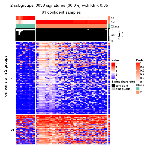
get_signatures(res, k = 2)
get_signatures(res, k = 3)
get_signatures(res, k = 4)
get_signatures(res, k = 5)
get_signatures(res, k = 6)
Signature heatmaps where rows are not scaled:
get_signatures(res, k = 2, scale_rows = FALSE)
get_signatures(res, k = 3, scale_rows = FALSE)
get_signatures(res, k = 4, scale_rows = FALSE)
get_signatures(res, k = 5, scale_rows = FALSE)
get_signatures(res, k = 6, scale_rows = FALSE)
Compare the overlap of signatures from different k:
compare_signatures(res)
get_signature() returns a data frame invisibly. TO get the list of signatures, the function
call should be assigned to a variable explicitly. In following code, if plot argument is set
to FALSE, no heatmap is plotted while only the differential analysis is performed.
# code only for demonstration
tb = get_signature(res, k = ..., plot = FALSE)
An example of the output of tb is:
#>   which_row         fdr    mean_1    mean_2 scaled_mean_1 scaled_mean_2 km
#> 1        38 0.042760348  8.373488  9.131774    -0.5533452     0.5164555  1
#> 2        40 0.018707592  7.106213  8.469186    -0.6173731     0.5762149  1
#> 3        55 0.019134737 10.221463 11.207825    -0.6159697     0.5749050  1
#> 4        59 0.006059896  5.921854  7.869574    -0.6899429     0.6439467  1
#> 5        60 0.018055526  8.928898 10.211722    -0.6204761     0.5791110  1
#> 6        98 0.009384629 15.714769 14.887706     0.6635654    -0.6193277  2
...
The columns in tb are:
which_row: row indices corresponding to the input matrix.fdr: FDR for the differential test. mean_x: The mean value in group x.scaled_mean_x: The mean value in group x after rows are scaled.km: Row groups if k-means clustering is applied to rows.UMAP plot which shows how samples are separated.
dimension_reduction(res, k = 2, method = "UMAP")
dimension_reduction(res, k = 3, method = "UMAP")
dimension_reduction(res, k = 4, method = "UMAP")
dimension_reduction(res, k = 5, method = "UMAP")
dimension_reduction(res, k = 6, method = "UMAP")
Following heatmap shows how subgroups are split when increasing k:
collect_classes(res)
If matrix rows can be associated to genes, consider to use functional_enrichment(res,
...) to perform function enrichment for the signature genes. See this vignette for more detailed explanations.
The object with results only for a single top-value method and a single partition method can be extracted as:
res = res_list["SD", "skmeans"]
# you can also extract it by
# res = res_list["SD:skmeans"]
A summary of res and all the functions that can be applied to it:
res
#> A 'ConsensusPartition' object with k = 2, 3, 4, 5, 6.
#>   On a matrix with 10126 rows and 62 columns.
#>   Top rows (1000, 2000, 3000, 4000, 5000) are extracted by 'SD' method.
#>   Subgroups are detected by 'skmeans' method.
#>   Performed in total 1250 partitions by row resampling.
#>   Best k for subgroups seems to be 3.
#>
#> Following methods can be applied to this 'ConsensusPartition' object:
#>  [1] "cola_report"             "collect_classes"         "collect_plots"
#>  [4] "collect_stats"           "colnames"                "compare_signatures"
#>  [7] "consensus_heatmap"       "dimension_reduction"     "functional_enrichment"
#> [10] "get_anno_col"            "get_anno"                "get_classes"
#> [13] "get_consensus"           "get_matrix"              "get_membership"
#> [16] "get_param"               "get_signatures"          "get_stats"
#> [19] "is_best_k"               "is_stable_k"             "membership_heatmap"
#> [22] "ncol"                    "nrow"                    "plot_ecdf"
#> [25] "rownames"                "select_partition_number" "show"
#> [28] "suggest_best_k"          "test_to_known_factors"
collect_plots() function collects all the plots made from res for all k (number of partitions)
into one single page to provide an easy and fast comparison between different k.
collect_plots(res)
The plots are:
k and the heatmap of
predicted classes for each k.k.k.k.All the plots in panels can be made by individual functions and they are plotted later in this section.
select_partition_number() produces several plots showing different
statistics for choosing “optimized” k. There are following statistics:
k;k, the area increased is defined as \(A_k - A_{k-1}\).The detailed explanations of these statistics can be found in the cola vignette.
Generally speaking, lower PAC score, higher mean silhouette score or higher
concordance corresponds to better partition. Rand index and Jaccard index
measure how similar the current partition is compared to partition with k-1.
If they are too similar, we won't accept k is better than k-1.
select_partition_number(res)
The numeric values for all these statistics can be obtained by get_stats().
get_stats(res)
#>   k 1-PAC mean_silhouette concordance area_increased  Rand Jaccard
#> 2 2 0.751           0.842       0.930         0.5057 0.492   0.492
#> 3 3 0.862           0.885       0.949         0.2733 0.772   0.576
#> 4 4 0.778           0.780       0.883         0.1305 0.882   0.681
#> 5 5 0.711           0.744       0.837         0.0555 0.939   0.783
#> 6 6 0.731           0.610       0.790         0.0326 0.995   0.977
suggest_best_k() suggests the best \(k\) based on these statistics. The rules are as follows:
suggest_best_k(res)
#> [1] 3
Following shows the table of the partitions (You need to click the show/hide
code output link to see it). The membership matrix (columns with name p*)
is inferred by
clue::cl_consensus()
function with the SE method. Basically the value in the membership matrix
represents the probability to belong to a certain group. The finall class
label for an item is determined with the group with highest probability it
belongs to.
In get_classes() function, the entropy is calculated from the membership
matrix and the silhouette score is calculated from the consensus matrix.
cbind(get_classes(res, k = 2), get_membership(res, k = 2))
#>            class entropy silhouette    p1    p2
#> SRR764776      1  0.0000      0.934 1.000 0.000
#> SRR764777      1  0.0000      0.934 1.000 0.000
#> SRR764778      1  0.0000      0.934 1.000 0.000
#> SRR764779      1  0.0000      0.934 1.000 0.000
#> SRR764780      1  0.0000      0.934 1.000 0.000
#> SRR764781      1  0.0000      0.934 1.000 0.000
#> SRR764782      1  0.0000      0.934 1.000 0.000
#> SRR764783      1  0.0000      0.934 1.000 0.000
#> SRR764784      1  0.0000      0.934 1.000 0.000
#> SRR764785      2  0.0000      0.922 0.000 1.000
#> SRR764786      2  0.0000      0.922 0.000 1.000
#> SRR764787      1  0.0376      0.930 0.996 0.004
#> SRR764788      1  0.0000      0.934 1.000 0.000
#> SRR764789      1  1.0000     -0.136 0.500 0.500
#> SRR764790      2  0.0000      0.922 0.000 1.000
#> SRR764791      1  0.5178      0.814 0.884 0.116
#> SRR764792      1  0.0000      0.934 1.000 0.000
#> SRR764793      1  0.0000      0.934 1.000 0.000
#> SRR764794      2  0.0000      0.922 0.000 1.000
#> SRR764795      1  0.0000      0.934 1.000 0.000
#> SRR764796      1  0.0000      0.934 1.000 0.000
#> SRR764797      1  0.0000      0.934 1.000 0.000
#> SRR764798      1  0.9754      0.331 0.592 0.408
#> SRR764799      1  0.0000      0.934 1.000 0.000
#> SRR764800      1  0.0000      0.934 1.000 0.000
#> SRR764801      1  0.9522      0.411 0.628 0.372
#> SRR764802      1  0.0000      0.934 1.000 0.000
#> SRR764803      1  0.0000      0.934 1.000 0.000
#> SRR764804      2  0.0000      0.922 0.000 1.000
#> SRR764805      2  0.0000      0.922 0.000 1.000
#> SRR764806      2  0.0000      0.922 0.000 1.000
#> SRR764807      2  0.0000      0.922 0.000 1.000
#> SRR764808      2  0.0000      0.922 0.000 1.000
#> SRR764809      2  0.0000      0.922 0.000 1.000
#> SRR764810      2  0.0000      0.922 0.000 1.000
#> SRR764811      2  0.0000      0.922 0.000 1.000
#> SRR764812      2  0.0000      0.922 0.000 1.000
#> SRR764813      2  0.0000      0.922 0.000 1.000
#> SRR764814      1  0.0000      0.934 1.000 0.000
#> SRR764815      1  0.9000      0.531 0.684 0.316
#> SRR764816      1  0.0000      0.934 1.000 0.000
#> SRR764817      1  0.0000      0.934 1.000 0.000
#> SRR1066622     2  0.9522      0.462 0.372 0.628
#> SRR1066623     2  0.9491      0.470 0.368 0.632
#> SRR1066624     1  0.0000      0.934 1.000 0.000
#> SRR1066625     1  0.0000      0.934 1.000 0.000
#> SRR1066626     2  0.1414      0.907 0.020 0.980
#> SRR1066627     2  0.9522      0.462 0.372 0.628
#> SRR1066628     2  0.9522      0.462 0.372 0.628
#> SRR1066629     2  0.9522      0.462 0.372 0.628
#> SRR1066630     2  0.0000      0.922 0.000 1.000
#> SRR1066631     2  0.8267      0.646 0.260 0.740
#> SRR1066632     2  0.0000      0.922 0.000 1.000
#> SRR1066633     2  0.0000      0.922 0.000 1.000
#> SRR1066634     2  0.0000      0.922 0.000 1.000
#> SRR1066635     2  0.0000      0.922 0.000 1.000
#> SRR1066636     2  0.0000      0.922 0.000 1.000
#> SRR1066637     2  0.0000      0.922 0.000 1.000
#> SRR1066638     2  0.0000      0.922 0.000 1.000
#> SRR1066639     2  0.0000      0.922 0.000 1.000
#> SRR1066640     2  0.0000      0.922 0.000 1.000
#> SRR1066641     2  0.0000      0.922 0.000 1.000
cbind(get_classes(res, k = 3), get_membership(res, k = 3))
#>            class entropy silhouette    p1    p2    p3
#> SRR764776      1  0.0000      0.966 1.000 0.000 0.000
#> SRR764777      1  0.0000      0.966 1.000 0.000 0.000
#> SRR764778      1  0.0000      0.966 1.000 0.000 0.000
#> SRR764779      1  0.0000      0.966 1.000 0.000 0.000
#> SRR764780      1  0.0000      0.966 1.000 0.000 0.000
#> SRR764781      1  0.0000      0.966 1.000 0.000 0.000
#> SRR764782      1  0.0237      0.963 0.996 0.000 0.004
#> SRR764783      1  0.0000      0.966 1.000 0.000 0.000
#> SRR764784      1  0.0424      0.961 0.992 0.000 0.008
#> SRR764785      2  0.1289      0.937 0.000 0.968 0.032
#> SRR764786      2  0.1031      0.943 0.000 0.976 0.024
#> SRR764787      1  0.6661      0.221 0.588 0.012 0.400
#> SRR764788      1  0.0000      0.966 1.000 0.000 0.000
#> SRR764789      3  0.4964      0.792 0.116 0.048 0.836
#> SRR764790      2  0.0424      0.952 0.000 0.992 0.008
#> SRR764791      3  0.7256      0.211 0.440 0.028 0.532
#> SRR764792      1  0.4731      0.793 0.840 0.032 0.128
#> SRR764793      1  0.1964      0.916 0.944 0.000 0.056
#> SRR764794      2  0.3551      0.839 0.000 0.868 0.132
#> SRR764795      1  0.0000      0.966 1.000 0.000 0.000
#> SRR764796      1  0.1289      0.941 0.968 0.000 0.032
#> SRR764797      1  0.0000      0.966 1.000 0.000 0.000
#> SRR764798      2  0.5623      0.598 0.280 0.716 0.004
#> SRR764799      1  0.0000      0.966 1.000 0.000 0.000
#> SRR764800      1  0.0000      0.966 1.000 0.000 0.000
#> SRR764801      2  0.6386      0.329 0.412 0.584 0.004
#> SRR764802      1  0.0000      0.966 1.000 0.000 0.000
#> SRR764803      1  0.0000      0.966 1.000 0.000 0.000
#> SRR764804      2  0.0237      0.952 0.000 0.996 0.004
#> SRR764805      2  0.0237      0.952 0.000 0.996 0.004
#> SRR764806      2  0.0237      0.950 0.000 0.996 0.004
#> SRR764807      2  0.0424      0.952 0.000 0.992 0.008
#> SRR764808      2  0.0424      0.952 0.000 0.992 0.008
#> SRR764809      2  0.0237      0.952 0.000 0.996 0.004
#> SRR764810      2  0.0237      0.952 0.000 0.996 0.004
#> SRR764811      2  0.0424      0.952 0.000 0.992 0.008
#> SRR764812      2  0.0424      0.952 0.000 0.992 0.008
#> SRR764813      2  0.0424      0.952 0.000 0.992 0.008
#> SRR764814      1  0.0000      0.966 1.000 0.000 0.000
#> SRR764815      3  0.8578      0.578 0.224 0.172 0.604
#> SRR764816      1  0.0000      0.966 1.000 0.000 0.000
#> SRR764817      1  0.0000      0.966 1.000 0.000 0.000
#> SRR1066622     3  0.0237      0.881 0.000 0.004 0.996
#> SRR1066623     3  0.0237      0.881 0.000 0.004 0.996
#> SRR1066624     3  0.5678      0.559 0.316 0.000 0.684
#> SRR1066625     3  0.0475      0.879 0.004 0.004 0.992
#> SRR1066626     3  0.0237      0.881 0.000 0.004 0.996
#> SRR1066627     3  0.0237      0.881 0.000 0.004 0.996
#> SRR1066628     3  0.0237      0.881 0.000 0.004 0.996
#> SRR1066629     3  0.0237      0.881 0.000 0.004 0.996
#> SRR1066630     2  0.3412      0.847 0.000 0.876 0.124
#> SRR1066631     3  0.0237      0.881 0.000 0.004 0.996
#> SRR1066632     2  0.0237      0.951 0.000 0.996 0.004
#> SRR1066633     2  0.0237      0.950 0.000 0.996 0.004
#> SRR1066634     2  0.0892      0.943 0.000 0.980 0.020
#> SRR1066635     2  0.0000      0.952 0.000 1.000 0.000
#> SRR1066636     2  0.0237      0.950 0.000 0.996 0.004
#> SRR1066637     2  0.0237      0.950 0.000 0.996 0.004
#> SRR1066638     2  0.0000      0.952 0.000 1.000 0.000
#> SRR1066639     2  0.0000      0.952 0.000 1.000 0.000
#> SRR1066640     2  0.0237      0.950 0.000 0.996 0.004
#> SRR1066641     2  0.0424      0.952 0.000 0.992 0.008
cbind(get_classes(res, k = 4), get_membership(res, k = 4))
#>            class entropy silhouette    p1    p2    p3    p4
#> SRR764776      1  0.0000     0.9191 1.000 0.000 0.000 0.000
#> SRR764777      1  0.0000     0.9191 1.000 0.000 0.000 0.000
#> SRR764778      1  0.0000     0.9191 1.000 0.000 0.000 0.000
#> SRR764779      1  0.0000     0.9191 1.000 0.000 0.000 0.000
#> SRR764780      1  0.0000     0.9191 1.000 0.000 0.000 0.000
#> SRR764781      1  0.0000     0.9191 1.000 0.000 0.000 0.000
#> SRR764782      1  0.1743     0.8992 0.940 0.000 0.056 0.004
#> SRR764783      1  0.0336     0.9180 0.992 0.000 0.008 0.000
#> SRR764784      1  0.1722     0.9011 0.944 0.000 0.048 0.008
#> SRR764785      2  0.1406     0.8738 0.000 0.960 0.024 0.016
#> SRR764786      2  0.1520     0.8699 0.000 0.956 0.024 0.020
#> SRR764787      1  0.9330    -0.0521 0.380 0.100 0.224 0.296
#> SRR764788      1  0.1209     0.9104 0.964 0.000 0.032 0.004
#> SRR764789      4  0.8885     0.3644 0.184 0.156 0.152 0.508
#> SRR764790      2  0.0188     0.8913 0.000 0.996 0.004 0.000
#> SRR764791      1  0.8953    -0.0207 0.392 0.060 0.240 0.308
#> SRR764792      1  0.6385     0.6385 0.676 0.024 0.224 0.076
#> SRR764793      1  0.3787     0.8258 0.840 0.000 0.124 0.036
#> SRR764794      2  0.4477     0.7129 0.000 0.808 0.084 0.108
#> SRR764795      1  0.1211     0.9081 0.960 0.000 0.040 0.000
#> SRR764796      1  0.2131     0.8911 0.932 0.000 0.032 0.036
#> SRR764797      1  0.0817     0.9151 0.976 0.000 0.024 0.000
#> SRR764798      3  0.3421     0.7280 0.088 0.044 0.868 0.000
#> SRR764799      1  0.0000     0.9191 1.000 0.000 0.000 0.000
#> SRR764800      1  0.0000     0.9191 1.000 0.000 0.000 0.000
#> SRR764801      3  0.3245     0.7132 0.100 0.028 0.872 0.000
#> SRR764802      1  0.0469     0.9172 0.988 0.000 0.012 0.000
#> SRR764803      1  0.0469     0.9177 0.988 0.000 0.012 0.000
#> SRR764804      2  0.0336     0.8906 0.000 0.992 0.008 0.000
#> SRR764805      2  0.2704     0.7829 0.000 0.876 0.124 0.000
#> SRR764806      3  0.4008     0.7767 0.000 0.244 0.756 0.000
#> SRR764807      2  0.0000     0.8926 0.000 1.000 0.000 0.000
#> SRR764808      2  0.0000     0.8926 0.000 1.000 0.000 0.000
#> SRR764809      2  0.1389     0.8656 0.000 0.952 0.048 0.000
#> SRR764810      2  0.0707     0.8864 0.000 0.980 0.020 0.000
#> SRR764811      2  0.0188     0.8917 0.000 0.996 0.004 0.000
#> SRR764812      2  0.0188     0.8920 0.000 0.996 0.004 0.000
#> SRR764813      2  0.0000     0.8926 0.000 1.000 0.000 0.000
#> SRR764814      1  0.0188     0.9183 0.996 0.000 0.004 0.000
#> SRR764815      3  0.9336     0.2465 0.184 0.152 0.440 0.224
#> SRR764816      1  0.0000     0.9191 1.000 0.000 0.000 0.000
#> SRR764817      1  0.0000     0.9191 1.000 0.000 0.000 0.000
#> SRR1066622     4  0.0188     0.8924 0.000 0.004 0.000 0.996
#> SRR1066623     4  0.0376     0.8914 0.000 0.004 0.004 0.992
#> SRR1066624     4  0.4936     0.4723 0.340 0.000 0.008 0.652
#> SRR1066625     4  0.0524     0.8873 0.004 0.000 0.008 0.988
#> SRR1066626     4  0.0188     0.8924 0.000 0.004 0.000 0.996
#> SRR1066627     4  0.0376     0.8914 0.000 0.004 0.004 0.992
#> SRR1066628     4  0.0188     0.8924 0.000 0.004 0.000 0.996
#> SRR1066629     4  0.0188     0.8924 0.000 0.004 0.000 0.996
#> SRR1066630     2  0.1743     0.8542 0.000 0.940 0.004 0.056
#> SRR1066631     4  0.0188     0.8924 0.000 0.004 0.000 0.996
#> SRR1066632     2  0.5290    -0.2101 0.000 0.516 0.476 0.008
#> SRR1066633     3  0.4252     0.7660 0.000 0.252 0.744 0.004
#> SRR1066634     3  0.4422     0.7625 0.000 0.256 0.736 0.008
#> SRR1066635     2  0.4356     0.4346 0.000 0.708 0.292 0.000
#> SRR1066636     3  0.3942     0.7808 0.000 0.236 0.764 0.000
#> SRR1066637     3  0.3907     0.7827 0.000 0.232 0.768 0.000
#> SRR1066638     3  0.4699     0.6963 0.000 0.320 0.676 0.004
#> SRR1066639     3  0.5112     0.4900 0.000 0.436 0.560 0.004
#> SRR1066640     3  0.3311     0.7838 0.000 0.172 0.828 0.000
#> SRR1066641     2  0.0000     0.8926 0.000 1.000 0.000 0.000
cbind(get_classes(res, k = 5), get_membership(res, k = 5))
#>            class entropy silhouette    p1    p2    p3    p4    p5
#> SRR764776      1  0.0000     0.9067 1.000 0.000 0.000 0.000 0.000
#> SRR764777      1  0.0000     0.9067 1.000 0.000 0.000 0.000 0.000
#> SRR764778      1  0.0000     0.9067 1.000 0.000 0.000 0.000 0.000
#> SRR764779      1  0.0000     0.9067 1.000 0.000 0.000 0.000 0.000
#> SRR764780      1  0.0000     0.9067 1.000 0.000 0.000 0.000 0.000
#> SRR764781      1  0.0162     0.9059 0.996 0.000 0.000 0.000 0.004
#> SRR764782      1  0.3883     0.7135 0.764 0.000 0.016 0.004 0.216
#> SRR764783      1  0.0703     0.9014 0.976 0.000 0.000 0.000 0.024
#> SRR764784      1  0.3427     0.7577 0.796 0.000 0.000 0.012 0.192
#> SRR764785      2  0.2689     0.8226 0.000 0.888 0.012 0.016 0.084
#> SRR764786      2  0.1956     0.8504 0.000 0.928 0.008 0.012 0.052
#> SRR764787      5  0.8027     0.5153 0.196 0.060 0.092 0.116 0.536
#> SRR764788      1  0.2074     0.8582 0.896 0.000 0.000 0.000 0.104
#> SRR764789      5  0.8481     0.3431 0.068 0.104 0.092 0.312 0.424
#> SRR764790      2  0.0566     0.8710 0.000 0.984 0.004 0.000 0.012
#> SRR764791      5  0.8180     0.5223 0.220 0.048 0.096 0.132 0.504
#> SRR764792      5  0.6948     0.4138 0.360 0.024 0.076 0.036 0.504
#> SRR764793      1  0.4931     0.3552 0.600 0.000 0.012 0.016 0.372
#> SRR764794      2  0.6315     0.4755 0.000 0.636 0.060 0.108 0.196
#> SRR764795      1  0.2723     0.8323 0.864 0.000 0.000 0.012 0.124
#> SRR764796      1  0.3170     0.8144 0.848 0.000 0.004 0.024 0.124
#> SRR764797      1  0.3999     0.6424 0.740 0.000 0.020 0.000 0.240
#> SRR764798      3  0.4586     0.5645 0.080 0.040 0.788 0.000 0.092
#> SRR764799      1  0.0324     0.9046 0.992 0.000 0.004 0.000 0.004
#> SRR764800      1  0.0000     0.9067 1.000 0.000 0.000 0.000 0.000
#> SRR764801      3  0.4194     0.5360 0.084 0.012 0.800 0.000 0.104
#> SRR764802      1  0.0703     0.9016 0.976 0.000 0.000 0.000 0.024
#> SRR764803      1  0.1043     0.8963 0.960 0.000 0.000 0.000 0.040
#> SRR764804      2  0.0609     0.8726 0.000 0.980 0.020 0.000 0.000
#> SRR764805      2  0.4162     0.6672 0.000 0.768 0.176 0.000 0.056
#> SRR764806      3  0.4801     0.6746 0.000 0.148 0.728 0.000 0.124
#> SRR764807      2  0.0290     0.8731 0.000 0.992 0.000 0.000 0.008
#> SRR764808      2  0.0290     0.8731 0.000 0.992 0.000 0.000 0.008
#> SRR764809      2  0.3242     0.7681 0.000 0.844 0.116 0.000 0.040
#> SRR764810      2  0.1809     0.8476 0.000 0.928 0.060 0.000 0.012
#> SRR764811      2  0.0992     0.8714 0.000 0.968 0.024 0.000 0.008
#> SRR764812      2  0.0451     0.8741 0.000 0.988 0.008 0.000 0.004
#> SRR764813      2  0.0290     0.8741 0.000 0.992 0.008 0.000 0.000
#> SRR764814      1  0.0451     0.9035 0.988 0.000 0.004 0.000 0.008
#> SRR764815      5  0.8790     0.2599 0.108 0.104 0.216 0.116 0.456
#> SRR764816      1  0.0324     0.9046 0.992 0.000 0.004 0.000 0.004
#> SRR764817      1  0.0324     0.9046 0.992 0.000 0.004 0.000 0.004
#> SRR1066622     4  0.0290     0.8988 0.000 0.000 0.000 0.992 0.008
#> SRR1066623     4  0.0404     0.8965 0.000 0.000 0.000 0.988 0.012
#> SRR1066624     4  0.4856     0.0241 0.388 0.000 0.000 0.584 0.028
#> SRR1066625     4  0.0798     0.8897 0.000 0.000 0.008 0.976 0.016
#> SRR1066626     4  0.0912     0.8849 0.000 0.012 0.000 0.972 0.016
#> SRR1066627     4  0.0290     0.8985 0.000 0.000 0.000 0.992 0.008
#> SRR1066628     4  0.0290     0.8988 0.000 0.000 0.000 0.992 0.008
#> SRR1066629     4  0.0290     0.8985 0.000 0.000 0.000 0.992 0.008
#> SRR1066630     2  0.1956     0.8299 0.000 0.916 0.000 0.076 0.008
#> SRR1066631     4  0.0404     0.8973 0.000 0.000 0.000 0.988 0.012
#> SRR1066632     3  0.6842     0.4494 0.000 0.344 0.404 0.004 0.248
#> SRR1066633     3  0.5192     0.6722 0.000 0.164 0.700 0.004 0.132
#> SRR1066634     3  0.6471     0.6135 0.000 0.184 0.564 0.016 0.236
#> SRR1066635     2  0.5246     0.2203 0.000 0.596 0.344 0.000 0.060
#> SRR1066636     3  0.4926     0.6792 0.000 0.176 0.712 0.000 0.112
#> SRR1066637     3  0.5481     0.6705 0.000 0.172 0.656 0.000 0.172
#> SRR1066638     3  0.6060     0.6435 0.000 0.228 0.592 0.004 0.176
#> SRR1066639     3  0.6407     0.5808 0.000 0.296 0.532 0.008 0.164
#> SRR1066640     3  0.5075     0.6742 0.000 0.124 0.720 0.008 0.148
#> SRR1066641     2  0.0510     0.8724 0.000 0.984 0.016 0.000 0.000
cbind(get_classes(res, k = 6), get_membership(res, k = 6))
#>            class entropy silhouette    p1    p2    p3    p4    p5    p6
#> SRR764776      1  0.0000    0.87067 1.000 0.000 0.000 0.000 0.000 0.000
#> SRR764777      1  0.0000    0.87067 1.000 0.000 0.000 0.000 0.000 0.000
#> SRR764778      1  0.0000    0.87067 1.000 0.000 0.000 0.000 0.000 0.000
#> SRR764779      1  0.0000    0.87067 1.000 0.000 0.000 0.000 0.000 0.000
#> SRR764780      1  0.0000    0.87067 1.000 0.000 0.000 0.000 0.000 0.000
#> SRR764781      1  0.0000    0.87067 1.000 0.000 0.000 0.000 0.000 0.000
#> SRR764782      1  0.4401    0.56927 0.660 0.000 0.012 0.000 0.300 0.028
#> SRR764783      1  0.0937    0.86237 0.960 0.000 0.000 0.000 0.040 0.000
#> SRR764784      1  0.4117    0.66290 0.716 0.000 0.004 0.004 0.244 0.032
#> SRR764785      2  0.3797    0.62848 0.000 0.800 0.004 0.008 0.112 0.076
#> SRR764786      2  0.2356    0.75254 0.000 0.900 0.004 0.004 0.048 0.044
#> SRR764787      5  0.6201    0.47207 0.120 0.032 0.024 0.036 0.660 0.128
#> SRR764788      1  0.3030    0.78198 0.816 0.000 0.008 0.000 0.168 0.008
#> SRR764789      5  0.8613    0.30888 0.060 0.100 0.056 0.200 0.420 0.164
#> SRR764790      2  0.0914    0.78353 0.000 0.968 0.000 0.000 0.016 0.016
#> SRR764791      5  0.7542    0.44838 0.132 0.016 0.044 0.100 0.524 0.184
#> SRR764792      5  0.7238    0.39431 0.332 0.004 0.040 0.036 0.424 0.164
#> SRR764793      1  0.5797   -0.00415 0.460 0.000 0.020 0.016 0.440 0.064
#> SRR764794      2  0.6622    0.14844 0.000 0.564 0.024 0.056 0.160 0.196
#> SRR764795      1  0.3122    0.76998 0.804 0.000 0.000 0.000 0.176 0.020
#> SRR764796      1  0.4175    0.73348 0.776 0.000 0.004 0.028 0.140 0.052
#> SRR764797      1  0.4886    0.53865 0.660 0.000 0.016 0.004 0.264 0.056
#> SRR764798      3  0.3884    0.42921 0.032 0.036 0.820 0.000 0.024 0.088
#> SRR764799      1  0.0622    0.86502 0.980 0.000 0.012 0.000 0.000 0.008
#> SRR764800      1  0.0000    0.87067 1.000 0.000 0.000 0.000 0.000 0.000
#> SRR764801      3  0.3807    0.43141 0.048 0.000 0.808 0.000 0.040 0.104
#> SRR764802      1  0.0865    0.86392 0.964 0.000 0.000 0.000 0.036 0.000
#> SRR764803      1  0.1625    0.85198 0.928 0.000 0.000 0.000 0.060 0.012
#> SRR764804      2  0.1745    0.76987 0.000 0.924 0.020 0.000 0.000 0.056
#> SRR764805      2  0.5220    0.31275 0.000 0.656 0.156 0.000 0.016 0.172
#> SRR764806      3  0.6171    0.28899 0.000 0.148 0.548 0.004 0.036 0.264
#> SRR764807      2  0.0622    0.78321 0.000 0.980 0.000 0.000 0.008 0.012
#> SRR764808      2  0.0260    0.78380 0.000 0.992 0.000 0.000 0.000 0.008
#> SRR764809      2  0.4396    0.56665 0.000 0.748 0.120 0.000 0.016 0.116
#> SRR764810      2  0.3200    0.70574 0.000 0.840 0.060 0.000 0.008 0.092
#> SRR764811      2  0.1649    0.77919 0.000 0.936 0.016 0.000 0.008 0.040
#> SRR764812      2  0.1462    0.77992 0.000 0.936 0.008 0.000 0.000 0.056
#> SRR764813      2  0.0891    0.78660 0.000 0.968 0.000 0.000 0.008 0.024
#> SRR764814      1  0.1458    0.84692 0.948 0.000 0.020 0.000 0.016 0.016
#> SRR764815      5  0.8636    0.23739 0.096 0.072 0.096 0.064 0.352 0.320
#> SRR764816      1  0.0508    0.86664 0.984 0.000 0.012 0.000 0.000 0.004
#> SRR764817      1  0.0405    0.86793 0.988 0.000 0.008 0.000 0.000 0.004
#> SRR1066622     4  0.0820    0.86826 0.000 0.000 0.000 0.972 0.012 0.016
#> SRR1066623     4  0.0363    0.86910 0.000 0.000 0.000 0.988 0.000 0.012
#> SRR1066624     4  0.5232   -0.03535 0.428 0.000 0.000 0.504 0.040 0.028
#> SRR1066625     4  0.1390    0.85707 0.000 0.000 0.004 0.948 0.032 0.016
#> SRR1066626     4  0.1959    0.84133 0.000 0.020 0.000 0.924 0.024 0.032
#> SRR1066627     4  0.0603    0.86849 0.000 0.000 0.000 0.980 0.016 0.004
#> SRR1066628     4  0.0622    0.86862 0.000 0.000 0.000 0.980 0.012 0.008
#> SRR1066629     4  0.1151    0.86018 0.000 0.000 0.000 0.956 0.032 0.012
#> SRR1066630     2  0.2692    0.72644 0.000 0.880 0.004 0.072 0.008 0.036
#> SRR1066631     4  0.1642    0.85296 0.000 0.000 0.004 0.936 0.032 0.028
#> SRR1066632     6  0.7260    0.00000 0.000 0.324 0.264 0.004 0.076 0.332
#> SRR1066633     3  0.6045    0.19587 0.000 0.172 0.592 0.000 0.056 0.180
#> SRR1066634     3  0.6666    0.33600 0.000 0.092 0.488 0.024 0.060 0.336
#> SRR1066635     2  0.5842    0.11816 0.000 0.596 0.212 0.000 0.036 0.156
#> SRR1066636     3  0.5660    0.33834 0.000 0.128 0.628 0.004 0.032 0.208
#> SRR1066637     3  0.5961    0.27733 0.000 0.132 0.544 0.000 0.032 0.292
#> SRR1066638     3  0.6964    0.18987 0.000 0.168 0.416 0.020 0.044 0.352
#> SRR1066639     3  0.7046   -0.17584 0.000 0.272 0.408 0.008 0.052 0.260
#> SRR1066640     3  0.5368    0.41692 0.000 0.048 0.624 0.000 0.060 0.268
#> SRR1066641     2  0.0665    0.78609 0.000 0.980 0.008 0.000 0.004 0.008
Heatmaps for the consensus matrix. It visualizes the probability of two samples to be in a same group.
consensus_heatmap(res, k = 2)
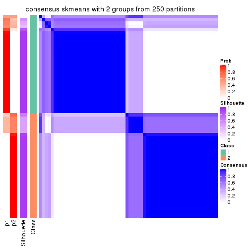
consensus_heatmap(res, k = 3)
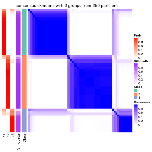
consensus_heatmap(res, k = 4)
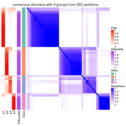
consensus_heatmap(res, k = 5)
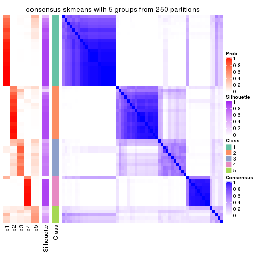
consensus_heatmap(res, k = 6)
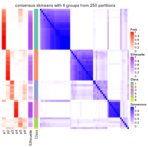
Heatmaps for the membership of samples in all partitions to see how consistent they are:
membership_heatmap(res, k = 2)
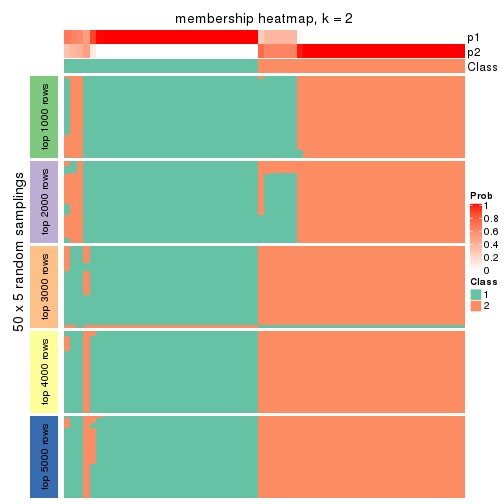
membership_heatmap(res, k = 3)
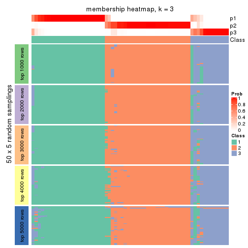
membership_heatmap(res, k = 4)
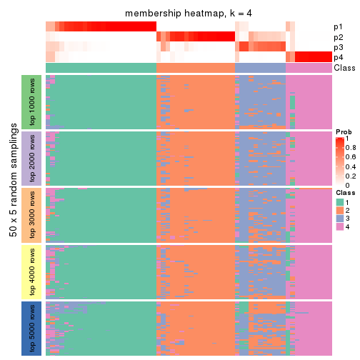
membership_heatmap(res, k = 5)
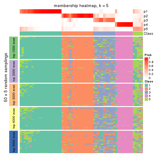
membership_heatmap(res, k = 6)
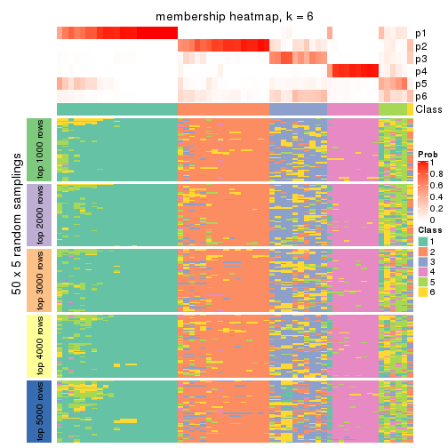
As soon as we have had the classes for columns, we can look for signatures which are significantly different between classes which can be candidate marks for certain classes. Following are the heatmaps for signatures.
Signature heatmaps where rows are scaled:
get_signatures(res, k = 2)
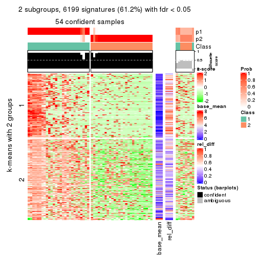
get_signatures(res, k = 3)
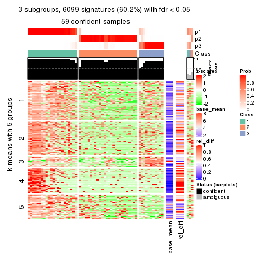
get_signatures(res, k = 4)
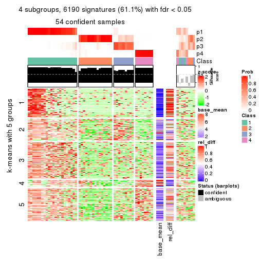
get_signatures(res, k = 5)
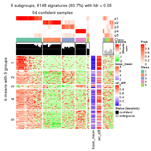
get_signatures(res, k = 6)
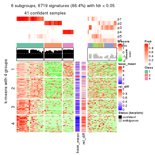
Signature heatmaps where rows are not scaled:
get_signatures(res, k = 2, scale_rows = FALSE)
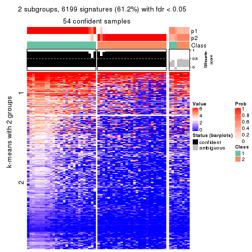
get_signatures(res, k = 3, scale_rows = FALSE)
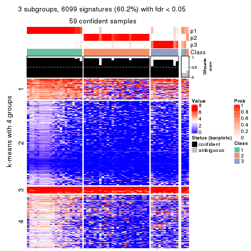
get_signatures(res, k = 4, scale_rows = FALSE)
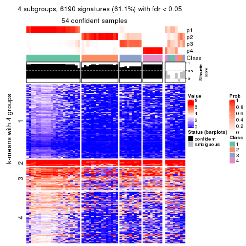
get_signatures(res, k = 5, scale_rows = FALSE)
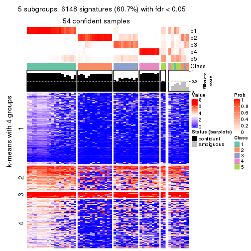
get_signatures(res, k = 6, scale_rows = FALSE)
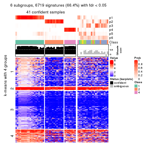
Compare the overlap of signatures from different k:
compare_signatures(res)
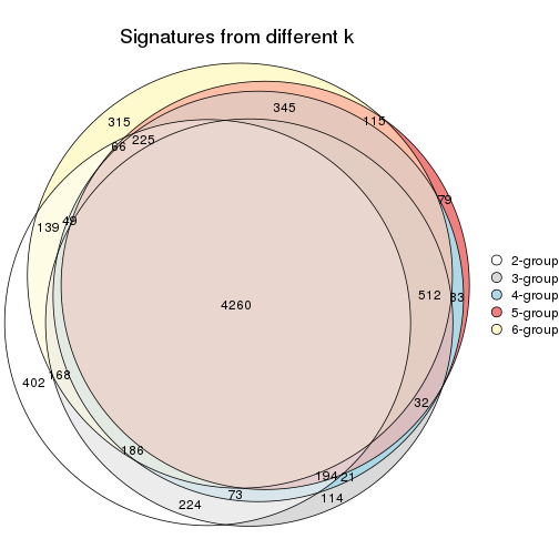
get_signature() returns a data frame invisibly. TO get the list of signatures, the function
call should be assigned to a variable explicitly. In following code, if plot argument is set
to FALSE, no heatmap is plotted while only the differential analysis is performed.
# code only for demonstration
tb = get_signature(res, k = ..., plot = FALSE)
An example of the output of tb is:
#>   which_row         fdr    mean_1    mean_2 scaled_mean_1 scaled_mean_2 km
#> 1        38 0.042760348  8.373488  9.131774    -0.5533452     0.5164555  1
#> 2        40 0.018707592  7.106213  8.469186    -0.6173731     0.5762149  1
#> 3        55 0.019134737 10.221463 11.207825    -0.6159697     0.5749050  1
#> 4        59 0.006059896  5.921854  7.869574    -0.6899429     0.6439467  1
#> 5        60 0.018055526  8.928898 10.211722    -0.6204761     0.5791110  1
#> 6        98 0.009384629 15.714769 14.887706     0.6635654    -0.6193277  2
...
The columns in tb are:
which_row: row indices corresponding to the input matrix.fdr: FDR for the differential test. mean_x: The mean value in group x.scaled_mean_x: The mean value in group x after rows are scaled.km: Row groups if k-means clustering is applied to rows.UMAP plot which shows how samples are separated.
dimension_reduction(res, k = 2, method = "UMAP")
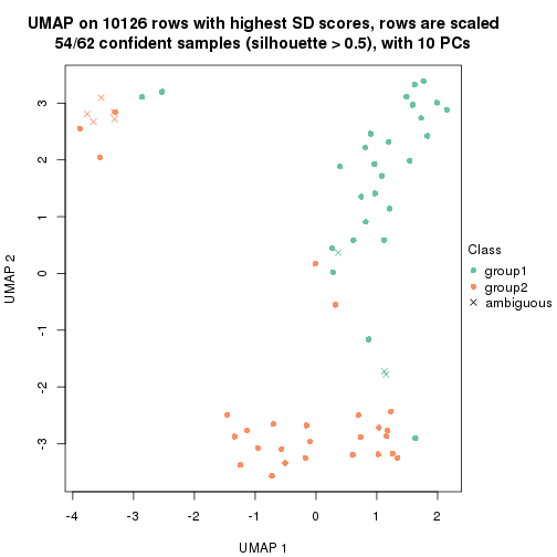
dimension_reduction(res, k = 3, method = "UMAP")
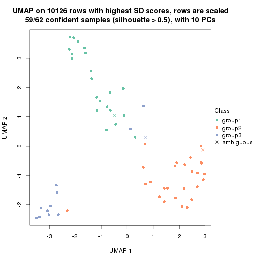
dimension_reduction(res, k = 4, method = "UMAP")
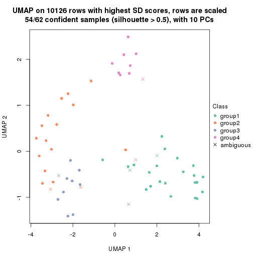
dimension_reduction(res, k = 5, method = "UMAP")
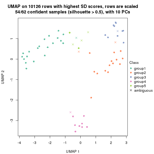
dimension_reduction(res, k = 6, method = "UMAP")
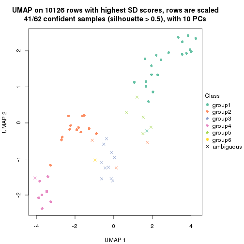
Following heatmap shows how subgroups are split when increasing k:
collect_classes(res)
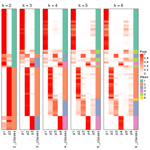
If matrix rows can be associated to genes, consider to use functional_enrichment(res,
...) to perform function enrichment for the signature genes. See this vignette for more detailed explanations.
The object with results only for a single top-value method and a single partition method can be extracted as:
res = res_list["SD", "pam"]
# you can also extract it by
# res = res_list["SD:pam"]
A summary of res and all the functions that can be applied to it:
res
#> A 'ConsensusPartition' object with k = 2, 3, 4, 5, 6.
#>   On a matrix with 10126 rows and 62 columns.
#>   Top rows (1000, 2000, 3000, 4000, 5000) are extracted by 'SD' method.
#>   Subgroups are detected by 'pam' method.
#>   Performed in total 1250 partitions by row resampling.
#>   Best k for subgroups seems to be 3.
#>
#> Following methods can be applied to this 'ConsensusPartition' object:
#>  [1] "cola_report"             "collect_classes"         "collect_plots"
#>  [4] "collect_stats"           "colnames"                "compare_signatures"
#>  [7] "consensus_heatmap"       "dimension_reduction"     "functional_enrichment"
#> [10] "get_anno_col"            "get_anno"                "get_classes"
#> [13] "get_consensus"           "get_matrix"              "get_membership"
#> [16] "get_param"               "get_signatures"          "get_stats"
#> [19] "is_best_k"               "is_stable_k"             "membership_heatmap"
#> [22] "ncol"                    "nrow"                    "plot_ecdf"
#> [25] "rownames"                "select_partition_number" "show"
#> [28] "suggest_best_k"          "test_to_known_factors"
collect_plots() function collects all the plots made from res for all k (number of partitions)
into one single page to provide an easy and fast comparison between different k.
collect_plots(res)
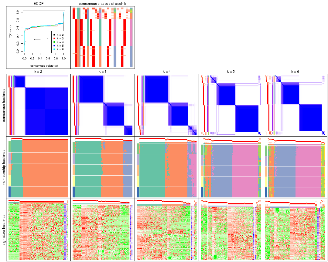
The plots are:
k and the heatmap of
predicted classes for each k.k.k.k.All the plots in panels can be made by individual functions and they are plotted later in this section.
select_partition_number() produces several plots showing different
statistics for choosing “optimized” k. There are following statistics:
k;k, the area increased is defined as \(A_k - A_{k-1}\).The detailed explanations of these statistics can be found in the cola vignette.
Generally speaking, lower PAC score, higher mean silhouette score or higher
concordance corresponds to better partition. Rand index and Jaccard index
measure how similar the current partition is compared to partition with k-1.
If they are too similar, we won't accept k is better than k-1.
select_partition_number(res)
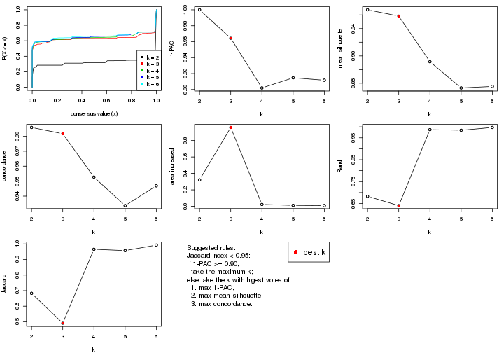
The numeric values for all these statistics can be obtained by get_stats().
get_stats(res)
#>   k 1-PAC mean_silhouette concordance area_increased  Rand Jaccard
#> 2 2 1.000           0.967       0.986        0.32119 0.683   0.683
#> 3 3 0.964           0.958       0.982        0.95941 0.640   0.491
#> 4 4 0.902           0.892       0.953        0.02273 0.987   0.966
#> 5 5 0.915           0.853       0.934        0.01131 0.985   0.957
#> 6 6 0.912           0.855       0.947        0.00861 0.997   0.992
suggest_best_k() suggests the best \(k\) based on these statistics. The rules are as follows:
suggest_best_k(res)
#> [1] 3
#> attr(,"optional")
#> [1] 2
There is also optional best \(k\) = 2 that is worth to check.
Following shows the table of the partitions (You need to click the show/hide
code output link to see it). The membership matrix (columns with name p*)
is inferred by
clue::cl_consensus()
function with the SE method. Basically the value in the membership matrix
represents the probability to belong to a certain group. The finall class
label for an item is determined with the group with highest probability it
belongs to.
In get_classes() function, the entropy is calculated from the membership
matrix and the silhouette score is calculated from the consensus matrix.
cbind(get_classes(res, k = 2), get_membership(res, k = 2))
#>            class entropy silhouette    p1    p2
#> SRR764776      2  0.0000      0.988 0.000 1.000
#> SRR764777      2  0.0000      0.988 0.000 1.000
#> SRR764778      2  0.0000      0.988 0.000 1.000
#> SRR764779      2  0.0000      0.988 0.000 1.000
#> SRR764780      2  0.0000      0.988 0.000 1.000
#> SRR764781      2  0.0000      0.988 0.000 1.000
#> SRR764782      2  0.0000      0.988 0.000 1.000
#> SRR764783      2  0.0000      0.988 0.000 1.000
#> SRR764784      2  0.0000      0.988 0.000 1.000
#> SRR764785      2  0.0672      0.987 0.008 0.992
#> SRR764786      1  0.0376      0.971 0.996 0.004
#> SRR764787      2  0.0000      0.988 0.000 1.000
#> SRR764788      2  0.0000      0.988 0.000 1.000
#> SRR764789      2  0.0672      0.987 0.008 0.992
#> SRR764790      1  0.0000      0.973 1.000 0.000
#> SRR764791      2  0.0672      0.987 0.008 0.992
#> SRR764792      2  0.0672      0.987 0.008 0.992
#> SRR764793      2  0.0000      0.988 0.000 1.000
#> SRR764794      2  0.0672      0.987 0.008 0.992
#> SRR764795      2  0.0000      0.988 0.000 1.000
#> SRR764796      2  0.0000      0.988 0.000 1.000
#> SRR764797      2  0.0000      0.988 0.000 1.000
#> SRR764798      2  0.0672      0.987 0.008 0.992
#> SRR764799      2  0.0672      0.987 0.008 0.992
#> SRR764800      2  0.0000      0.988 0.000 1.000
#> SRR764801      2  0.0672      0.987 0.008 0.992
#> SRR764802      2  0.0000      0.988 0.000 1.000
#> SRR764803      2  0.0000      0.988 0.000 1.000
#> SRR764804      1  0.0000      0.973 1.000 0.000
#> SRR764805      2  0.9775      0.275 0.412 0.588
#> SRR764806      2  0.0672      0.987 0.008 0.992
#> SRR764807      1  0.0000      0.973 1.000 0.000
#> SRR764808      1  0.0000      0.973 1.000 0.000
#> SRR764809      1  0.2043      0.948 0.968 0.032
#> SRR764810      1  0.8144      0.659 0.748 0.252
#> SRR764811      1  0.0000      0.973 1.000 0.000
#> SRR764812      1  0.0000      0.973 1.000 0.000
#> SRR764813      1  0.0000      0.973 1.000 0.000
#> SRR764814      2  0.0672      0.987 0.008 0.992
#> SRR764815      2  0.0672      0.987 0.008 0.992
#> SRR764816      2  0.0672      0.987 0.008 0.992
#> SRR764817      2  0.0672      0.987 0.008 0.992
#> SRR1066622     2  0.0000      0.988 0.000 1.000
#> SRR1066623     2  0.0000      0.988 0.000 1.000
#> SRR1066624     2  0.0000      0.988 0.000 1.000
#> SRR1066625     2  0.0000      0.988 0.000 1.000
#> SRR1066626     2  0.0000      0.988 0.000 1.000
#> SRR1066627     2  0.0000      0.988 0.000 1.000
#> SRR1066628     2  0.0000      0.988 0.000 1.000
#> SRR1066629     2  0.0000      0.988 0.000 1.000
#> SRR1066630     1  0.0000      0.973 1.000 0.000
#> SRR1066631     2  0.0000      0.988 0.000 1.000
#> SRR1066632     2  0.0672      0.987 0.008 0.992
#> SRR1066633     2  0.0672      0.987 0.008 0.992
#> SRR1066634     2  0.0672      0.987 0.008 0.992
#> SRR1066635     2  0.0672      0.987 0.008 0.992
#> SRR1066636     2  0.0672      0.987 0.008 0.992
#> SRR1066637     2  0.0672      0.987 0.008 0.992
#> SRR1066638     2  0.0672      0.987 0.008 0.992
#> SRR1066639     2  0.0672      0.987 0.008 0.992
#> SRR1066640     2  0.0672      0.987 0.008 0.992
#> SRR1066641     1  0.0000      0.973 1.000 0.000
cbind(get_classes(res, k = 3), get_membership(res, k = 3))
#>            class entropy silhouette    p1    p2    p3
#> SRR764776      1  0.0000      0.993 1.000 0.000 0.000
#> SRR764777      1  0.0000      0.993 1.000 0.000 0.000
#> SRR764778      1  0.0000      0.993 1.000 0.000 0.000
#> SRR764779      1  0.0000      0.993 1.000 0.000 0.000
#> SRR764780      1  0.0000      0.993 1.000 0.000 0.000
#> SRR764781      1  0.0000      0.993 1.000 0.000 0.000
#> SRR764782      1  0.0000      0.993 1.000 0.000 0.000
#> SRR764783      1  0.0000      0.993 1.000 0.000 0.000
#> SRR764784      1  0.0000      0.993 1.000 0.000 0.000
#> SRR764785      2  0.0000      0.962 0.000 1.000 0.000
#> SRR764786      3  0.3267      0.879 0.000 0.116 0.884
#> SRR764787      1  0.0000      0.993 1.000 0.000 0.000
#> SRR764788      1  0.0000      0.993 1.000 0.000 0.000
#> SRR764789      2  0.0000      0.962 0.000 1.000 0.000
#> SRR764790      3  0.0000      0.972 0.000 0.000 1.000
#> SRR764791      1  0.3941      0.800 0.844 0.156 0.000
#> SRR764792      2  0.3816      0.791 0.148 0.852 0.000
#> SRR764793      1  0.0000      0.993 1.000 0.000 0.000
#> SRR764794      2  0.0592      0.951 0.012 0.988 0.000
#> SRR764795      1  0.0000      0.993 1.000 0.000 0.000
#> SRR764796      1  0.0000      0.993 1.000 0.000 0.000
#> SRR764797      1  0.0000      0.993 1.000 0.000 0.000
#> SRR764798      2  0.0000      0.962 0.000 1.000 0.000
#> SRR764799      2  0.0000      0.962 0.000 1.000 0.000
#> SRR764800      1  0.0000      0.993 1.000 0.000 0.000
#> SRR764801      2  0.0000      0.962 0.000 1.000 0.000
#> SRR764802      1  0.0000      0.993 1.000 0.000 0.000
#> SRR764803      1  0.0000      0.993 1.000 0.000 0.000
#> SRR764804      3  0.1529      0.954 0.000 0.040 0.960
#> SRR764805      2  0.0000      0.962 0.000 1.000 0.000
#> SRR764806      2  0.0000      0.962 0.000 1.000 0.000
#> SRR764807      3  0.0000      0.972 0.000 0.000 1.000
#> SRR764808      3  0.0000      0.972 0.000 0.000 1.000
#> SRR764809      2  0.3192      0.858 0.000 0.888 0.112
#> SRR764810      2  0.3551      0.835 0.000 0.868 0.132
#> SRR764811      3  0.0424      0.971 0.000 0.008 0.992
#> SRR764812      3  0.2356      0.928 0.000 0.072 0.928
#> SRR764813      3  0.0000      0.972 0.000 0.000 1.000
#> SRR764814      2  0.5678      0.540 0.316 0.684 0.000
#> SRR764815      2  0.0000      0.962 0.000 1.000 0.000
#> SRR764816      2  0.0000      0.962 0.000 1.000 0.000
#> SRR764817      2  0.0000      0.962 0.000 1.000 0.000
#> SRR1066622     1  0.0000      0.993 1.000 0.000 0.000
#> SRR1066623     1  0.0000      0.993 1.000 0.000 0.000
#> SRR1066624     1  0.0237      0.989 0.996 0.004 0.000
#> SRR1066625     1  0.0000      0.993 1.000 0.000 0.000
#> SRR1066626     1  0.0237      0.989 0.996 0.004 0.000
#> SRR1066627     1  0.0000      0.993 1.000 0.000 0.000
#> SRR1066628     1  0.0237      0.989 0.996 0.004 0.000
#> SRR1066629     1  0.0000      0.993 1.000 0.000 0.000
#> SRR1066630     3  0.0592      0.970 0.000 0.012 0.988
#> SRR1066631     1  0.0000      0.993 1.000 0.000 0.000
#> SRR1066632     2  0.0000      0.962 0.000 1.000 0.000
#> SRR1066633     2  0.0000      0.962 0.000 1.000 0.000
#> SRR1066634     2  0.0000      0.962 0.000 1.000 0.000
#> SRR1066635     2  0.0000      0.962 0.000 1.000 0.000
#> SRR1066636     2  0.0000      0.962 0.000 1.000 0.000
#> SRR1066637     2  0.0000      0.962 0.000 1.000 0.000
#> SRR1066638     2  0.0000      0.962 0.000 1.000 0.000
#> SRR1066639     2  0.0000      0.962 0.000 1.000 0.000
#> SRR1066640     2  0.0000      0.962 0.000 1.000 0.000
#> SRR1066641     3  0.0000      0.972 0.000 0.000 1.000
cbind(get_classes(res, k = 4), get_membership(res, k = 4))
#>            class entropy silhouette    p1    p2    p3    p4
#> SRR764776      1  0.0000      0.992 1.000 0.000 0.000 0.000
#> SRR764777      1  0.0000      0.992 1.000 0.000 0.000 0.000
#> SRR764778      1  0.0000      0.992 1.000 0.000 0.000 0.000
#> SRR764779      1  0.0000      0.992 1.000 0.000 0.000 0.000
#> SRR764780      1  0.0000      0.992 1.000 0.000 0.000 0.000
#> SRR764781      1  0.0000      0.992 1.000 0.000 0.000 0.000
#> SRR764782      1  0.0000      0.992 1.000 0.000 0.000 0.000
#> SRR764783      1  0.0000      0.992 1.000 0.000 0.000 0.000
#> SRR764784      1  0.0000      0.992 1.000 0.000 0.000 0.000
#> SRR764785      2  0.0000      0.954 0.000 1.000 0.000 0.000
#> SRR764786      4  0.2983      0.685 0.000 0.040 0.068 0.892
#> SRR764787      1  0.0000      0.992 1.000 0.000 0.000 0.000
#> SRR764788      1  0.0000      0.992 1.000 0.000 0.000 0.000
#> SRR764789      2  0.0000      0.954 0.000 1.000 0.000 0.000
#> SRR764790      4  0.0188      0.737 0.000 0.000 0.004 0.996
#> SRR764791      1  0.3123      0.780 0.844 0.156 0.000 0.000
#> SRR764792      2  0.3024      0.767 0.148 0.852 0.000 0.000
#> SRR764793      1  0.0000      0.992 1.000 0.000 0.000 0.000
#> SRR764794      2  0.0469      0.942 0.012 0.988 0.000 0.000
#> SRR764795      1  0.0000      0.992 1.000 0.000 0.000 0.000
#> SRR764796      1  0.0000      0.992 1.000 0.000 0.000 0.000
#> SRR764797      1  0.0000      0.992 1.000 0.000 0.000 0.000
#> SRR764798      2  0.0000      0.954 0.000 1.000 0.000 0.000
#> SRR764799      2  0.0000      0.954 0.000 1.000 0.000 0.000
#> SRR764800      1  0.0000      0.992 1.000 0.000 0.000 0.000
#> SRR764801      2  0.0000      0.954 0.000 1.000 0.000 0.000
#> SRR764802      1  0.0000      0.992 1.000 0.000 0.000 0.000
#> SRR764803      1  0.0000      0.992 1.000 0.000 0.000 0.000
#> SRR764804      3  0.4252      0.673 0.000 0.004 0.744 0.252
#> SRR764805      2  0.0000      0.954 0.000 1.000 0.000 0.000
#> SRR764806      2  0.0000      0.954 0.000 1.000 0.000 0.000
#> SRR764807      4  0.4103      0.543 0.000 0.000 0.256 0.744
#> SRR764808      4  0.0188      0.737 0.000 0.000 0.004 0.996
#> SRR764809      2  0.3808      0.763 0.000 0.812 0.176 0.012
#> SRR764810      2  0.3718      0.771 0.000 0.820 0.168 0.012
#> SRR764811      3  0.1302      0.630 0.000 0.000 0.956 0.044
#> SRR764812      3  0.4535      0.678 0.000 0.016 0.744 0.240
#> SRR764813      4  0.4624      0.190 0.000 0.000 0.340 0.660
#> SRR764814      2  0.4500      0.481 0.316 0.684 0.000 0.000
#> SRR764815      2  0.0000      0.954 0.000 1.000 0.000 0.000
#> SRR764816      2  0.0000      0.954 0.000 1.000 0.000 0.000
#> SRR764817      2  0.0000      0.954 0.000 1.000 0.000 0.000
#> SRR1066622     1  0.0000      0.992 1.000 0.000 0.000 0.000
#> SRR1066623     1  0.0000      0.992 1.000 0.000 0.000 0.000
#> SRR1066624     1  0.0188      0.988 0.996 0.004 0.000 0.000
#> SRR1066625     1  0.0000      0.992 1.000 0.000 0.000 0.000
#> SRR1066626     1  0.0188      0.988 0.996 0.004 0.000 0.000
#> SRR1066627     1  0.0000      0.992 1.000 0.000 0.000 0.000
#> SRR1066628     1  0.0188      0.988 0.996 0.004 0.000 0.000
#> SRR1066629     1  0.0000      0.992 1.000 0.000 0.000 0.000
#> SRR1066630     4  0.3355      0.661 0.000 0.004 0.160 0.836
#> SRR1066631     1  0.0000      0.992 1.000 0.000 0.000 0.000
#> SRR1066632     2  0.0000      0.954 0.000 1.000 0.000 0.000
#> SRR1066633     2  0.0000      0.954 0.000 1.000 0.000 0.000
#> SRR1066634     2  0.0000      0.954 0.000 1.000 0.000 0.000
#> SRR1066635     2  0.0000      0.954 0.000 1.000 0.000 0.000
#> SRR1066636     2  0.0000      0.954 0.000 1.000 0.000 0.000
#> SRR1066637     2  0.0000      0.954 0.000 1.000 0.000 0.000
#> SRR1066638     2  0.0000      0.954 0.000 1.000 0.000 0.000
#> SRR1066639     2  0.0000      0.954 0.000 1.000 0.000 0.000
#> SRR1066640     2  0.0000      0.954 0.000 1.000 0.000 0.000
#> SRR1066641     3  0.4713      0.326 0.000 0.000 0.640 0.360
cbind(get_classes(res, k = 5), get_membership(res, k = 5))
#>            class entropy silhouette    p1    p2    p3    p4    p5
#> SRR764776      4  0.0000     0.9920 0.000 0.000 0.000 1.000 0.000
#> SRR764777      4  0.0000     0.9920 0.000 0.000 0.000 1.000 0.000
#> SRR764778      4  0.0000     0.9920 0.000 0.000 0.000 1.000 0.000
#> SRR764779      4  0.0000     0.9920 0.000 0.000 0.000 1.000 0.000
#> SRR764780      4  0.0000     0.9920 0.000 0.000 0.000 1.000 0.000
#> SRR764781      4  0.0000     0.9920 0.000 0.000 0.000 1.000 0.000
#> SRR764782      4  0.0000     0.9920 0.000 0.000 0.000 1.000 0.000
#> SRR764783      4  0.0000     0.9920 0.000 0.000 0.000 1.000 0.000
#> SRR764784      4  0.0000     0.9920 0.000 0.000 0.000 1.000 0.000
#> SRR764785      3  0.0000     0.9518 0.000 0.000 1.000 0.000 0.000
#> SRR764786      2  0.3353     0.7108 0.024 0.852 0.020 0.000 0.104
#> SRR764787      4  0.0000     0.9920 0.000 0.000 0.000 1.000 0.000
#> SRR764788      4  0.0000     0.9920 0.000 0.000 0.000 1.000 0.000
#> SRR764789      3  0.0000     0.9518 0.000 0.000 1.000 0.000 0.000
#> SRR764790      2  0.0000     0.7666 0.000 1.000 0.000 0.000 0.000
#> SRR764791      4  0.2690     0.7734 0.000 0.000 0.156 0.844 0.000
#> SRR764792      3  0.2605     0.7159 0.000 0.000 0.852 0.148 0.000
#> SRR764793      4  0.0000     0.9920 0.000 0.000 0.000 1.000 0.000
#> SRR764794      3  0.0404     0.9367 0.000 0.000 0.988 0.012 0.000
#> SRR764795      4  0.0000     0.9920 0.000 0.000 0.000 1.000 0.000
#> SRR764796      4  0.0000     0.9920 0.000 0.000 0.000 1.000 0.000
#> SRR764797      4  0.0000     0.9920 0.000 0.000 0.000 1.000 0.000
#> SRR764798      3  0.0000     0.9518 0.000 0.000 1.000 0.000 0.000
#> SRR764799      3  0.0000     0.9518 0.000 0.000 1.000 0.000 0.000
#> SRR764800      4  0.0000     0.9920 0.000 0.000 0.000 1.000 0.000
#> SRR764801      3  0.0000     0.9518 0.000 0.000 1.000 0.000 0.000
#> SRR764802      4  0.0000     0.9920 0.000 0.000 0.000 1.000 0.000
#> SRR764803      4  0.0000     0.9920 0.000 0.000 0.000 1.000 0.000
#> SRR764804      5  0.6416    -0.2306 0.356 0.180 0.000 0.000 0.464
#> SRR764805      3  0.0000     0.9518 0.000 0.000 1.000 0.000 0.000
#> SRR764806      3  0.0000     0.9518 0.000 0.000 1.000 0.000 0.000
#> SRR764807      2  0.4558     0.6449 0.088 0.744 0.000 0.000 0.168
#> SRR764808      2  0.0000     0.7666 0.000 1.000 0.000 0.000 0.000
#> SRR764809      3  0.3772     0.6593 0.036 0.000 0.792 0.000 0.172
#> SRR764810      5  0.4294    -0.0959 0.000 0.000 0.468 0.000 0.532
#> SRR764811      1  0.4382     0.5346 0.688 0.024 0.000 0.000 0.288
#> SRR764812      5  0.6535    -0.2267 0.356 0.176 0.004 0.000 0.464
#> SRR764813      2  0.5215     0.4188 0.240 0.664 0.000 0.000 0.096
#> SRR764814      3  0.3876     0.3801 0.000 0.000 0.684 0.316 0.000
#> SRR764815      3  0.0000     0.9518 0.000 0.000 1.000 0.000 0.000
#> SRR764816      3  0.0000     0.9518 0.000 0.000 1.000 0.000 0.000
#> SRR764817      3  0.0000     0.9518 0.000 0.000 1.000 0.000 0.000
#> SRR1066622     4  0.0000     0.9920 0.000 0.000 0.000 1.000 0.000
#> SRR1066623     4  0.0000     0.9920 0.000 0.000 0.000 1.000 0.000
#> SRR1066624     4  0.0162     0.9879 0.000 0.000 0.004 0.996 0.000
#> SRR1066625     4  0.0000     0.9920 0.000 0.000 0.000 1.000 0.000
#> SRR1066626     4  0.0162     0.9880 0.000 0.000 0.004 0.996 0.000
#> SRR1066627     4  0.0000     0.9920 0.000 0.000 0.000 1.000 0.000
#> SRR1066628     4  0.0162     0.9878 0.000 0.000 0.004 0.996 0.000
#> SRR1066629     4  0.0000     0.9920 0.000 0.000 0.000 1.000 0.000
#> SRR1066630     2  0.3519     0.6963 0.008 0.776 0.000 0.000 0.216
#> SRR1066631     4  0.0000     0.9920 0.000 0.000 0.000 1.000 0.000
#> SRR1066632     3  0.0000     0.9518 0.000 0.000 1.000 0.000 0.000
#> SRR1066633     3  0.0000     0.9518 0.000 0.000 1.000 0.000 0.000
#> SRR1066634     3  0.0000     0.9518 0.000 0.000 1.000 0.000 0.000
#> SRR1066635     3  0.0000     0.9518 0.000 0.000 1.000 0.000 0.000
#> SRR1066636     3  0.0000     0.9518 0.000 0.000 1.000 0.000 0.000
#> SRR1066637     3  0.0000     0.9518 0.000 0.000 1.000 0.000 0.000
#> SRR1066638     3  0.0000     0.9518 0.000 0.000 1.000 0.000 0.000
#> SRR1066639     3  0.0000     0.9518 0.000 0.000 1.000 0.000 0.000
#> SRR1066640     3  0.0000     0.9518 0.000 0.000 1.000 0.000 0.000
#> SRR1066641     1  0.2329     0.5883 0.876 0.124 0.000 0.000 0.000
cbind(get_classes(res, k = 6), get_membership(res, k = 6))
#>            class entropy silhouette    p1    p2    p3    p4    p5    p6
#> SRR764776      4  0.0000      0.992 0.000 0.000 0.000 1.000 0.000 0.000
#> SRR764777      4  0.0000      0.992 0.000 0.000 0.000 1.000 0.000 0.000
#> SRR764778      4  0.0000      0.992 0.000 0.000 0.000 1.000 0.000 0.000
#> SRR764779      4  0.0000      0.992 0.000 0.000 0.000 1.000 0.000 0.000
#> SRR764780      4  0.0000      0.992 0.000 0.000 0.000 1.000 0.000 0.000
#> SRR764781      4  0.0000      0.992 0.000 0.000 0.000 1.000 0.000 0.000
#> SRR764782      4  0.0000      0.992 0.000 0.000 0.000 1.000 0.000 0.000
#> SRR764783      4  0.0000      0.992 0.000 0.000 0.000 1.000 0.000 0.000
#> SRR764784      4  0.0000      0.992 0.000 0.000 0.000 1.000 0.000 0.000
#> SRR764785      3  0.0000      0.949 0.000 0.000 1.000 0.000 0.000 0.000
#> SRR764786      2  0.3670      0.672 0.024 0.832 0.020 0.000 0.084 0.040
#> SRR764787      4  0.0000      0.992 0.000 0.000 0.000 1.000 0.000 0.000
#> SRR764788      4  0.0000      0.992 0.000 0.000 0.000 1.000 0.000 0.000
#> SRR764789      3  0.0000      0.949 0.000 0.000 1.000 0.000 0.000 0.000
#> SRR764790      2  0.0000      0.737 0.000 1.000 0.000 0.000 0.000 0.000
#> SRR764791      4  0.2416      0.765 0.000 0.000 0.156 0.844 0.000 0.000
#> SRR764792      3  0.2340      0.702 0.000 0.000 0.852 0.148 0.000 0.000
#> SRR764793      4  0.0000      0.992 0.000 0.000 0.000 1.000 0.000 0.000
#> SRR764794      3  0.0363      0.934 0.000 0.000 0.988 0.012 0.000 0.000
#> SRR764795      4  0.0000      0.992 0.000 0.000 0.000 1.000 0.000 0.000
#> SRR764796      4  0.0000      0.992 0.000 0.000 0.000 1.000 0.000 0.000
#> SRR764797      4  0.0000      0.992 0.000 0.000 0.000 1.000 0.000 0.000
#> SRR764798      3  0.0000      0.949 0.000 0.000 1.000 0.000 0.000 0.000
#> SRR764799      3  0.0000      0.949 0.000 0.000 1.000 0.000 0.000 0.000
#> SRR764800      4  0.0000      0.992 0.000 0.000 0.000 1.000 0.000 0.000
#> SRR764801      3  0.0000      0.949 0.000 0.000 1.000 0.000 0.000 0.000
#> SRR764802      4  0.0000      0.992 0.000 0.000 0.000 1.000 0.000 0.000
#> SRR764803      4  0.0000      0.992 0.000 0.000 0.000 1.000 0.000 0.000
#> SRR764804      5  0.2135      0.646 0.000 0.128 0.000 0.000 0.872 0.000
#> SRR764805      3  0.0000      0.949 0.000 0.000 1.000 0.000 0.000 0.000
#> SRR764806      3  0.0000      0.949 0.000 0.000 1.000 0.000 0.000 0.000
#> SRR764807      2  0.3175      0.591 0.000 0.744 0.000 0.000 0.256 0.000
#> SRR764808      2  0.0000      0.737 0.000 1.000 0.000 0.000 0.000 0.000
#> SRR764809      3  0.3201      0.630 0.012 0.000 0.780 0.000 0.208 0.000
#> SRR764810      1  0.3752      0.000 0.772 0.000 0.164 0.000 0.064 0.000
#> SRR764811      5  0.5316     -0.126 0.060 0.020 0.000 0.000 0.524 0.396
#> SRR764812      5  0.2135      0.646 0.000 0.128 0.000 0.000 0.872 0.000
#> SRR764813      2  0.5229      0.380 0.076 0.608 0.000 0.000 0.296 0.020
#> SRR764814      3  0.3482      0.334 0.000 0.000 0.684 0.316 0.000 0.000
#> SRR764815      3  0.0000      0.949 0.000 0.000 1.000 0.000 0.000 0.000
#> SRR764816      3  0.0000      0.949 0.000 0.000 1.000 0.000 0.000 0.000
#> SRR764817      3  0.0000      0.949 0.000 0.000 1.000 0.000 0.000 0.000
#> SRR1066622     4  0.0000      0.992 0.000 0.000 0.000 1.000 0.000 0.000
#> SRR1066623     4  0.0000      0.992 0.000 0.000 0.000 1.000 0.000 0.000
#> SRR1066624     4  0.0146      0.988 0.000 0.000 0.004 0.996 0.000 0.000
#> SRR1066625     4  0.0000      0.992 0.000 0.000 0.000 1.000 0.000 0.000
#> SRR1066626     4  0.0146      0.988 0.000 0.000 0.004 0.996 0.000 0.000
#> SRR1066627     4  0.0000      0.992 0.000 0.000 0.000 1.000 0.000 0.000
#> SRR1066628     4  0.0146      0.988 0.000 0.000 0.004 0.996 0.000 0.000
#> SRR1066629     4  0.0000      0.992 0.000 0.000 0.000 1.000 0.000 0.000
#> SRR1066630     2  0.5558      0.575 0.056 0.652 0.000 0.000 0.176 0.116
#> SRR1066631     4  0.0000      0.992 0.000 0.000 0.000 1.000 0.000 0.000
#> SRR1066632     3  0.0000      0.949 0.000 0.000 1.000 0.000 0.000 0.000
#> SRR1066633     3  0.0000      0.949 0.000 0.000 1.000 0.000 0.000 0.000
#> SRR1066634     3  0.0000      0.949 0.000 0.000 1.000 0.000 0.000 0.000
#> SRR1066635     3  0.0000      0.949 0.000 0.000 1.000 0.000 0.000 0.000
#> SRR1066636     3  0.0000      0.949 0.000 0.000 1.000 0.000 0.000 0.000
#> SRR1066637     3  0.0000      0.949 0.000 0.000 1.000 0.000 0.000 0.000
#> SRR1066638     3  0.0000      0.949 0.000 0.000 1.000 0.000 0.000 0.000
#> SRR1066639     3  0.0000      0.949 0.000 0.000 1.000 0.000 0.000 0.000
#> SRR1066640     3  0.0000      0.949 0.000 0.000 1.000 0.000 0.000 0.000
#> SRR1066641     6  0.4156      0.000 0.000 0.080 0.000 0.000 0.188 0.732
Heatmaps for the consensus matrix. It visualizes the probability of two samples to be in a same group.
consensus_heatmap(res, k = 2)
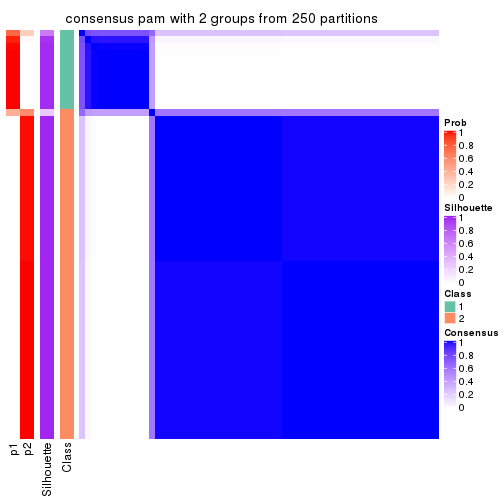
consensus_heatmap(res, k = 3)
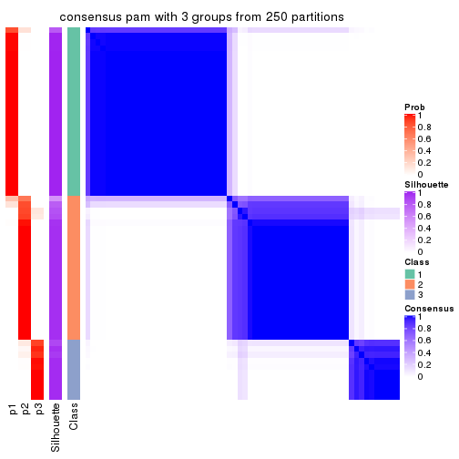
consensus_heatmap(res, k = 4)
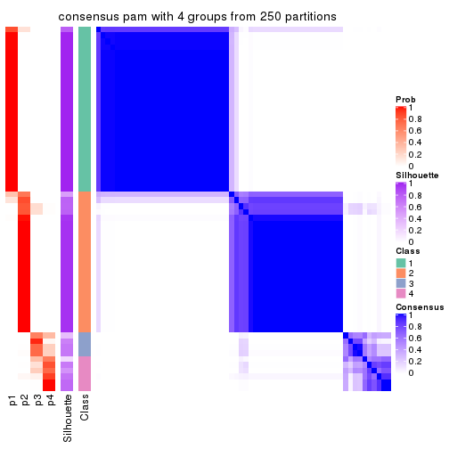
consensus_heatmap(res, k = 5)
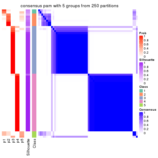
consensus_heatmap(res, k = 6)
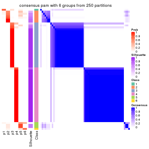
Heatmaps for the membership of samples in all partitions to see how consistent they are:
membership_heatmap(res, k = 2)

membership_heatmap(res, k = 3)
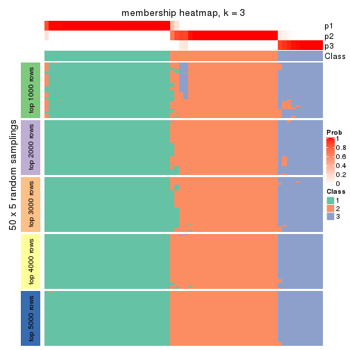
membership_heatmap(res, k = 4)
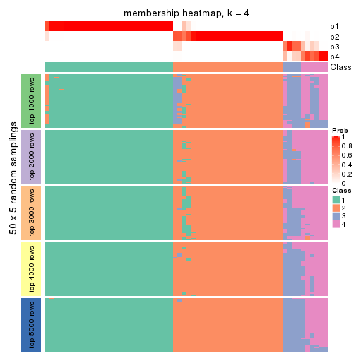
membership_heatmap(res, k = 5)
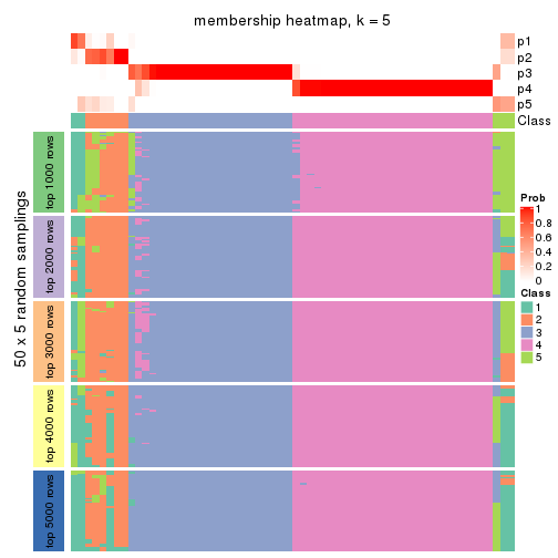
membership_heatmap(res, k = 6)
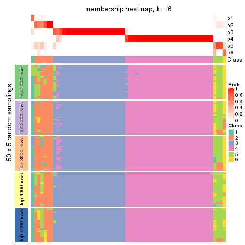
As soon as we have had the classes for columns, we can look for signatures which are significantly different between classes which can be candidate marks for certain classes. Following are the heatmaps for signatures.
Signature heatmaps where rows are scaled:
get_signatures(res, k = 2)
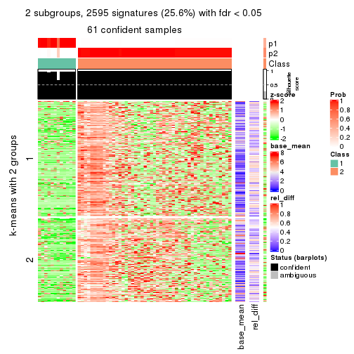
get_signatures(res, k = 3)
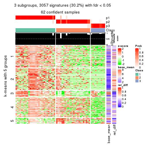
get_signatures(res, k = 4)
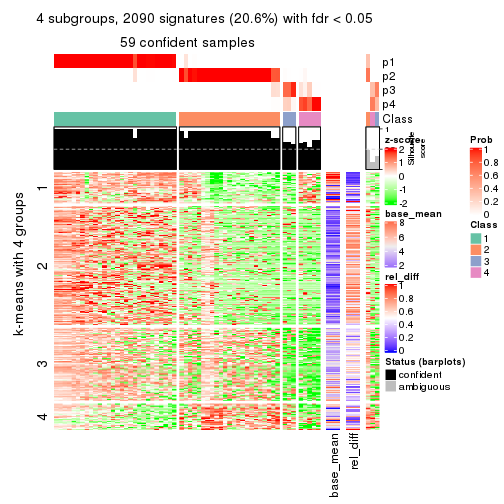
get_signatures(res, k = 5)
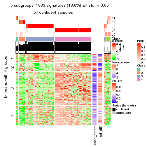
get_signatures(res, k = 6)
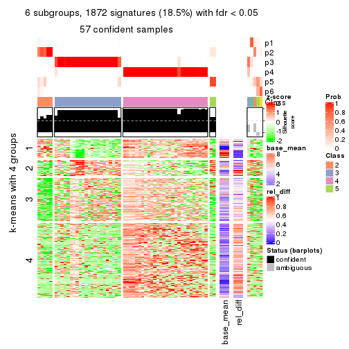
Signature heatmaps where rows are not scaled:
get_signatures(res, k = 2, scale_rows = FALSE)
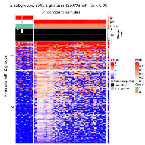
get_signatures(res, k = 3, scale_rows = FALSE)
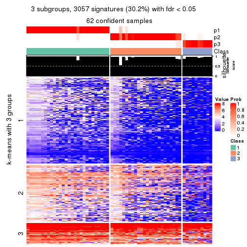
get_signatures(res, k = 4, scale_rows = FALSE)
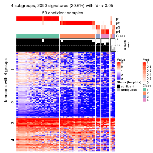
get_signatures(res, k = 5, scale_rows = FALSE)
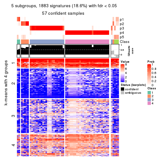
get_signatures(res, k = 6, scale_rows = FALSE)
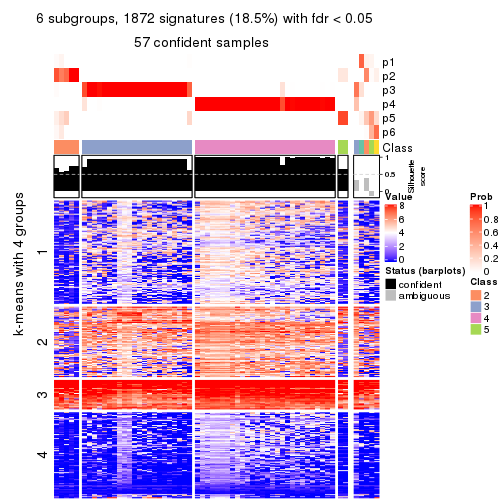
Compare the overlap of signatures from different k:
compare_signatures(res)
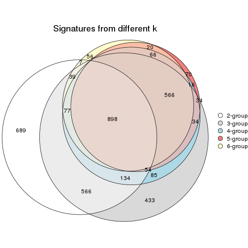
get_signature() returns a data frame invisibly. TO get the list of signatures, the function
call should be assigned to a variable explicitly. In following code, if plot argument is set
to FALSE, no heatmap is plotted while only the differential analysis is performed.
# code only for demonstration
tb = get_signature(res, k = ..., plot = FALSE)
An example of the output of tb is:
#>   which_row         fdr    mean_1    mean_2 scaled_mean_1 scaled_mean_2 km
#> 1        38 0.042760348  8.373488  9.131774    -0.5533452     0.5164555  1
#> 2        40 0.018707592  7.106213  8.469186    -0.6173731     0.5762149  1
#> 3        55 0.019134737 10.221463 11.207825    -0.6159697     0.5749050  1
#> 4        59 0.006059896  5.921854  7.869574    -0.6899429     0.6439467  1
#> 5        60 0.018055526  8.928898 10.211722    -0.6204761     0.5791110  1
#> 6        98 0.009384629 15.714769 14.887706     0.6635654    -0.6193277  2
...
The columns in tb are:
which_row: row indices corresponding to the input matrix.fdr: FDR for the differential test. mean_x: The mean value in group x.scaled_mean_x: The mean value in group x after rows are scaled.km: Row groups if k-means clustering is applied to rows.UMAP plot which shows how samples are separated.
dimension_reduction(res, k = 2, method = "UMAP")

dimension_reduction(res, k = 3, method = "UMAP")
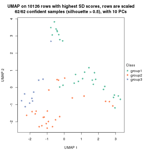
dimension_reduction(res, k = 4, method = "UMAP")
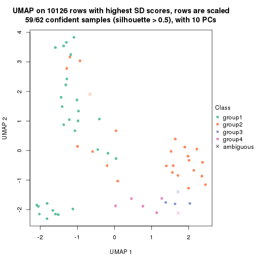
dimension_reduction(res, k = 5, method = "UMAP")
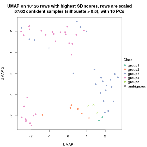
dimension_reduction(res, k = 6, method = "UMAP")
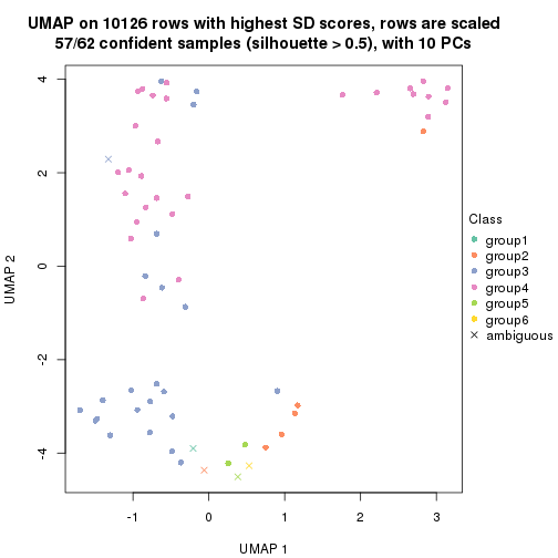
Following heatmap shows how subgroups are split when increasing k:
collect_classes(res)
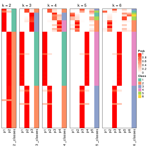
If matrix rows can be associated to genes, consider to use functional_enrichment(res,
...) to perform function enrichment for the signature genes. See this vignette for more detailed explanations.
The object with results only for a single top-value method and a single partition method can be extracted as:
res = res_list["SD", "mclust"]
# you can also extract it by
# res = res_list["SD:mclust"]
A summary of res and all the functions that can be applied to it:
res
#> A 'ConsensusPartition' object with k = 2, 3, 4, 5, 6.
#>   On a matrix with 10126 rows and 62 columns.
#>   Top rows (1000, 2000, 3000, 4000, 5000) are extracted by 'SD' method.
#>   Subgroups are detected by 'mclust' method.
#>   Performed in total 1250 partitions by row resampling.
#>   Best k for subgroups seems to be 3.
#>
#> Following methods can be applied to this 'ConsensusPartition' object:
#>  [1] "cola_report"             "collect_classes"         "collect_plots"
#>  [4] "collect_stats"           "colnames"                "compare_signatures"
#>  [7] "consensus_heatmap"       "dimension_reduction"     "functional_enrichment"
#> [10] "get_anno_col"            "get_anno"                "get_classes"
#> [13] "get_consensus"           "get_matrix"              "get_membership"
#> [16] "get_param"               "get_signatures"          "get_stats"
#> [19] "is_best_k"               "is_stable_k"             "membership_heatmap"
#> [22] "ncol"                    "nrow"                    "plot_ecdf"
#> [25] "rownames"                "select_partition_number" "show"
#> [28] "suggest_best_k"          "test_to_known_factors"
collect_plots() function collects all the plots made from res for all k (number of partitions)
into one single page to provide an easy and fast comparison between different k.
collect_plots(res)
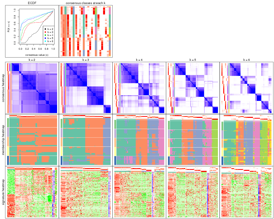
The plots are:
k and the heatmap of
predicted classes for each k.k.k.k.All the plots in panels can be made by individual functions and they are plotted later in this section.
select_partition_number() produces several plots showing different
statistics for choosing “optimized” k. There are following statistics:
k;k, the area increased is defined as \(A_k - A_{k-1}\).The detailed explanations of these statistics can be found in the cola vignette.
Generally speaking, lower PAC score, higher mean silhouette score or higher
concordance corresponds to better partition. Rand index and Jaccard index
measure how similar the current partition is compared to partition with k-1.
If they are too similar, we won't accept k is better than k-1.
select_partition_number(res)
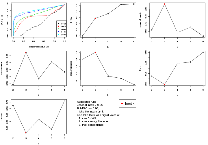
The numeric values for all these statistics can be obtained by get_stats().
get_stats(res)
#>   k 1-PAC mean_silhouette concordance area_increased  Rand Jaccard
#> 2 2 0.185           0.661       0.777         0.4029 0.725   0.725
#> 3 3 0.483           0.834       0.870         0.5044 0.647   0.513
#> 4 4 0.560           0.642       0.793         0.1580 0.846   0.616
#> 5 5 0.714           0.677       0.843         0.1247 0.859   0.541
#> 6 6 0.724           0.618       0.813         0.0364 0.950   0.761
suggest_best_k() suggests the best \(k\) based on these statistics. The rules are as follows:
suggest_best_k(res)
#> [1] 3
Following shows the table of the partitions (You need to click the show/hide
code output link to see it). The membership matrix (columns with name p*)
is inferred by
clue::cl_consensus()
function with the SE method. Basically the value in the membership matrix
represents the probability to belong to a certain group. The finall class
label for an item is determined with the group with highest probability it
belongs to.
In get_classes() function, the entropy is calculated from the membership
matrix and the silhouette score is calculated from the consensus matrix.
cbind(get_classes(res, k = 2), get_membership(res, k = 2))
#>            class entropy silhouette    p1    p2
#> SRR764776      2  0.9833      0.629 0.424 0.576
#> SRR764777      2  0.9833      0.629 0.424 0.576
#> SRR764778      2  0.9833      0.629 0.424 0.576
#> SRR764779      2  0.9833      0.629 0.424 0.576
#> SRR764780      2  0.9833      0.629 0.424 0.576
#> SRR764781      2  0.9833      0.629 0.424 0.576
#> SRR764782      2  0.8661      0.697 0.288 0.712
#> SRR764783      2  0.9393      0.675 0.356 0.644
#> SRR764784      2  0.8608      0.698 0.284 0.716
#> SRR764785      2  0.9248      0.609 0.340 0.660
#> SRR764786      2  0.9170      0.610 0.332 0.668
#> SRR764787      2  0.8661      0.696 0.288 0.712
#> SRR764788      2  0.8763      0.694 0.296 0.704
#> SRR764789      2  0.8555      0.699 0.280 0.720
#> SRR764790      2  0.9686     -0.180 0.396 0.604
#> SRR764791      2  0.8499      0.701 0.276 0.724
#> SRR764792      2  0.8608      0.696 0.284 0.716
#> SRR764793      2  0.8661      0.697 0.288 0.712
#> SRR764794      2  0.9248      0.674 0.340 0.660
#> SRR764795      2  0.8608      0.698 0.284 0.716
#> SRR764796      2  0.9522      0.584 0.372 0.628
#> SRR764797      2  0.9850      0.626 0.428 0.572
#> SRR764798      2  0.8499      0.577 0.276 0.724
#> SRR764799      2  0.9286      0.666 0.344 0.656
#> SRR764800      2  0.9815      0.632 0.420 0.580
#> SRR764801      2  0.8499      0.577 0.276 0.724
#> SRR764802      2  0.9833      0.629 0.424 0.576
#> SRR764803      2  0.9833      0.629 0.424 0.576
#> SRR764804      2  0.0000      0.670 0.000 1.000
#> SRR764805      2  0.2603      0.651 0.044 0.956
#> SRR764806      2  0.4690      0.611 0.100 0.900
#> SRR764807      2  0.8661      0.178 0.288 0.712
#> SRR764808      2  0.9661     -0.220 0.392 0.608
#> SRR764809      2  0.2043      0.658 0.032 0.968
#> SRR764810      2  0.2236      0.656 0.036 0.964
#> SRR764811      2  0.0376      0.672 0.004 0.996
#> SRR764812      2  0.0376      0.672 0.004 0.996
#> SRR764813      2  0.4298      0.642 0.088 0.912
#> SRR764814      2  0.9248      0.667 0.340 0.660
#> SRR764815      2  0.8207      0.709 0.256 0.744
#> SRR764816      2  0.9248      0.667 0.340 0.660
#> SRR764817      2  0.9248      0.667 0.340 0.660
#> SRR1066622     1  0.6343      0.962 0.840 0.160
#> SRR1066623     1  0.6343      0.962 0.840 0.160
#> SRR1066624     1  0.6438      0.925 0.836 0.164
#> SRR1066625     1  0.6712      0.940 0.824 0.176
#> SRR1066626     1  0.6343      0.962 0.840 0.160
#> SRR1066627     1  0.6343      0.962 0.840 0.160
#> SRR1066628     1  0.6343      0.962 0.840 0.160
#> SRR1066629     1  0.6343      0.962 0.840 0.160
#> SRR1066630     1  0.9000      0.717 0.684 0.316
#> SRR1066631     1  0.6343      0.962 0.840 0.160
#> SRR1066632     2  0.2603      0.656 0.044 0.956
#> SRR1066633     2  0.2948      0.654 0.052 0.948
#> SRR1066634     2  0.4298      0.623 0.088 0.912
#> SRR1066635     2  0.3431      0.639 0.064 0.936
#> SRR1066636     2  0.3431      0.642 0.064 0.936
#> SRR1066637     2  0.3879      0.633 0.076 0.924
#> SRR1066638     2  0.4431      0.620 0.092 0.908
#> SRR1066639     2  0.3431      0.639 0.064 0.936
#> SRR1066640     2  0.4815      0.608 0.104 0.896
#> SRR1066641     2  0.0000      0.670 0.000 1.000
cbind(get_classes(res, k = 3), get_membership(res, k = 3))
#>            class entropy silhouette    p1    p2    p3
#> SRR764776      1  0.0475      0.850 0.992 0.004 0.004
#> SRR764777      1  0.0475      0.850 0.992 0.004 0.004
#> SRR764778      1  0.0475      0.850 0.992 0.004 0.004
#> SRR764779      1  0.0475      0.850 0.992 0.004 0.004
#> SRR764780      1  0.0237      0.849 0.996 0.000 0.004
#> SRR764781      1  0.0237      0.849 0.996 0.000 0.004
#> SRR764782      1  0.5191      0.828 0.828 0.060 0.112
#> SRR764783      1  0.2443      0.854 0.940 0.028 0.032
#> SRR764784      1  0.4397      0.820 0.856 0.028 0.116
#> SRR764785      1  0.7338      0.621 0.652 0.288 0.060
#> SRR764786      1  0.7739      0.618 0.644 0.268 0.088
#> SRR764787      1  0.7192      0.782 0.716 0.164 0.120
#> SRR764788      1  0.4489      0.833 0.856 0.036 0.108
#> SRR764789      1  0.6438      0.770 0.748 0.188 0.064
#> SRR764790      2  0.6599      0.754 0.168 0.748 0.084
#> SRR764791      1  0.6892      0.791 0.736 0.152 0.112
#> SRR764792      1  0.6424      0.783 0.752 0.180 0.068
#> SRR764793      1  0.4786      0.826 0.844 0.044 0.112
#> SRR764794      1  0.7664      0.649 0.668 0.228 0.104
#> SRR764795      1  0.4136      0.821 0.864 0.020 0.116
#> SRR764796      1  0.5798      0.782 0.780 0.044 0.176
#> SRR764797      1  0.4591      0.819 0.848 0.120 0.032
#> SRR764798      2  0.6576      0.754 0.192 0.740 0.068
#> SRR764799      1  0.3886      0.830 0.880 0.096 0.024
#> SRR764800      1  0.1267      0.852 0.972 0.024 0.004
#> SRR764801      2  0.6576      0.754 0.192 0.740 0.068
#> SRR764802      1  0.1289      0.847 0.968 0.000 0.032
#> SRR764803      1  0.1711      0.851 0.960 0.008 0.032
#> SRR764804      2  0.2774      0.894 0.072 0.920 0.008
#> SRR764805      2  0.0592      0.901 0.012 0.988 0.000
#> SRR764806      2  0.0747      0.896 0.000 0.984 0.016
#> SRR764807      2  0.5105      0.832 0.124 0.828 0.048
#> SRR764808      2  0.5998      0.801 0.128 0.788 0.084
#> SRR764809      2  0.0747      0.902 0.016 0.984 0.000
#> SRR764810      2  0.1643      0.901 0.044 0.956 0.000
#> SRR764811      2  0.2774      0.894 0.072 0.920 0.008
#> SRR764812      2  0.2774      0.894 0.072 0.920 0.008
#> SRR764813      2  0.5307      0.822 0.136 0.816 0.048
#> SRR764814      1  0.2663      0.848 0.932 0.044 0.024
#> SRR764815      1  0.6154      0.739 0.752 0.204 0.044
#> SRR764816      1  0.2773      0.848 0.928 0.048 0.024
#> SRR764817      1  0.2663      0.848 0.932 0.044 0.024
#> SRR1066622     3  0.3192      0.902 0.112 0.000 0.888
#> SRR1066623     3  0.3192      0.902 0.112 0.000 0.888
#> SRR1066624     3  0.8156      0.725 0.196 0.160 0.644
#> SRR1066625     3  0.7412      0.771 0.176 0.124 0.700
#> SRR1066626     3  0.3425      0.901 0.112 0.004 0.884
#> SRR1066627     3  0.3192      0.902 0.112 0.000 0.888
#> SRR1066628     3  0.3192      0.902 0.112 0.000 0.888
#> SRR1066629     3  0.3192      0.902 0.112 0.000 0.888
#> SRR1066630     3  0.8511      0.583 0.152 0.244 0.604
#> SRR1066631     3  0.3192      0.902 0.112 0.000 0.888
#> SRR1066632     2  0.2031      0.900 0.032 0.952 0.016
#> SRR1066633     2  0.2902      0.899 0.064 0.920 0.016
#> SRR1066634     2  0.0747      0.896 0.000 0.984 0.016
#> SRR1066635     2  0.0747      0.896 0.000 0.984 0.016
#> SRR1066636     2  0.0983      0.898 0.004 0.980 0.016
#> SRR1066637     2  0.0747      0.896 0.000 0.984 0.016
#> SRR1066638     2  0.0747      0.896 0.000 0.984 0.016
#> SRR1066639     2  0.0747      0.896 0.000 0.984 0.016
#> SRR1066640     2  0.0747      0.896 0.000 0.984 0.016
#> SRR1066641     2  0.2774      0.894 0.072 0.920 0.008
cbind(get_classes(res, k = 4), get_membership(res, k = 4))
#>            class entropy silhouette    p1    p2    p3    p4
#> SRR764776      1  0.2844      0.790 0.900 0.000 0.048 0.052
#> SRR764777      1  0.2844      0.790 0.900 0.000 0.048 0.052
#> SRR764778      1  0.2844      0.790 0.900 0.000 0.048 0.052
#> SRR764779      1  0.2844      0.790 0.900 0.000 0.048 0.052
#> SRR764780      1  0.2469      0.803 0.892 0.000 0.108 0.000
#> SRR764781      1  0.3356      0.793 0.824 0.000 0.176 0.000
#> SRR764782      1  0.4288      0.757 0.828 0.004 0.084 0.084
#> SRR764783      1  0.3893      0.787 0.796 0.000 0.196 0.008
#> SRR764784      1  0.3266      0.770 0.880 0.004 0.032 0.084
#> SRR764785      3  0.3126      0.613 0.092 0.016 0.884 0.008
#> SRR764786      3  0.2837      0.616 0.068 0.012 0.904 0.016
#> SRR764787      1  0.6988      0.146 0.476 0.020 0.440 0.064
#> SRR764788      1  0.3852      0.762 0.800 0.000 0.192 0.008
#> SRR764789      1  0.5576      0.266 0.496 0.012 0.488 0.004
#> SRR764790      3  0.2450      0.627 0.000 0.072 0.912 0.016
#> SRR764791      1  0.5739      0.669 0.716 0.008 0.200 0.076
#> SRR764792      1  0.5679      0.319 0.492 0.016 0.488 0.004
#> SRR764793      1  0.4298      0.761 0.832 0.008 0.080 0.080
#> SRR764794      3  0.4584      0.481 0.196 0.016 0.776 0.012
#> SRR764795      1  0.3030      0.774 0.892 0.004 0.028 0.076
#> SRR764796      1  0.5752      0.673 0.720 0.008 0.084 0.188
#> SRR764797      1  0.4621      0.725 0.708 0.000 0.284 0.008
#> SRR764798      2  0.6011      0.547 0.132 0.688 0.180 0.000
#> SRR764799      1  0.3695      0.779 0.828 0.016 0.156 0.000
#> SRR764800      1  0.3457      0.792 0.876 0.008 0.076 0.040
#> SRR764801      2  0.6086      0.539 0.132 0.680 0.188 0.000
#> SRR764802      1  0.3725      0.792 0.812 0.000 0.180 0.008
#> SRR764803      1  0.3768      0.790 0.808 0.000 0.184 0.008
#> SRR764804      3  0.4916      0.266 0.000 0.424 0.576 0.000
#> SRR764805      2  0.4008      0.634 0.000 0.756 0.244 0.000
#> SRR764806      2  0.0188      0.805 0.000 0.996 0.004 0.000
#> SRR764807      3  0.2999      0.609 0.000 0.132 0.864 0.004
#> SRR764808      3  0.2796      0.623 0.000 0.092 0.892 0.016
#> SRR764809      2  0.4454      0.519 0.000 0.692 0.308 0.000
#> SRR764810      2  0.4855      0.256 0.000 0.600 0.400 0.000
#> SRR764811      3  0.4948      0.228 0.000 0.440 0.560 0.000
#> SRR764812      3  0.4866      0.316 0.000 0.404 0.596 0.000
#> SRR764813      3  0.4053      0.556 0.000 0.228 0.768 0.004
#> SRR764814      1  0.3335      0.792 0.856 0.016 0.128 0.000
#> SRR764815      3  0.5778     -0.317 0.472 0.028 0.500 0.000
#> SRR764816      1  0.3390      0.790 0.852 0.016 0.132 0.000
#> SRR764817      1  0.3390      0.790 0.852 0.016 0.132 0.000
#> SRR1066622     4  0.1474      0.921 0.000 0.000 0.052 0.948
#> SRR1066623     4  0.1474      0.921 0.000 0.000 0.052 0.948
#> SRR1066624     3  0.7403      0.113 0.152 0.004 0.488 0.356
#> SRR1066625     4  0.6405      0.146 0.056 0.004 0.420 0.520
#> SRR1066626     4  0.2053      0.899 0.004 0.000 0.072 0.924
#> SRR1066627     4  0.1474      0.921 0.000 0.000 0.052 0.948
#> SRR1066628     4  0.1474      0.921 0.000 0.000 0.052 0.948
#> SRR1066629     4  0.1474      0.921 0.000 0.000 0.052 0.948
#> SRR1066630     3  0.5481      0.261 0.020 0.004 0.628 0.348
#> SRR1066631     4  0.1474      0.921 0.000 0.000 0.052 0.948
#> SRR1066632     2  0.3810      0.676 0.008 0.804 0.188 0.000
#> SRR1066633     2  0.1940      0.774 0.000 0.924 0.076 0.000
#> SRR1066634     2  0.0000      0.805 0.000 1.000 0.000 0.000
#> SRR1066635     2  0.3123      0.725 0.000 0.844 0.156 0.000
#> SRR1066636     2  0.0469      0.805 0.000 0.988 0.012 0.000
#> SRR1066637     2  0.0000      0.805 0.000 1.000 0.000 0.000
#> SRR1066638     2  0.0000      0.805 0.000 1.000 0.000 0.000
#> SRR1066639     2  0.0000      0.805 0.000 1.000 0.000 0.000
#> SRR1066640     2  0.0000      0.805 0.000 1.000 0.000 0.000
#> SRR1066641     3  0.4916      0.265 0.000 0.424 0.576 0.000
cbind(get_classes(res, k = 5), get_membership(res, k = 5))
#>            class entropy silhouette    p1    p2    p3    p4    p5
#> SRR764776      1  0.0000    0.77953 1.000 0.000 0.000 0.000 0.000
#> SRR764777      1  0.0000    0.77953 1.000 0.000 0.000 0.000 0.000
#> SRR764778      1  0.0404    0.78155 0.988 0.000 0.000 0.012 0.000
#> SRR764779      1  0.0404    0.78155 0.988 0.000 0.000 0.012 0.000
#> SRR764780      1  0.3012    0.72566 0.852 0.024 0.000 0.124 0.000
#> SRR764781      1  0.3628    0.63528 0.772 0.012 0.000 0.216 0.000
#> SRR764782      4  0.3480    0.58537 0.248 0.000 0.000 0.752 0.000
#> SRR764783      1  0.4288    0.47411 0.664 0.012 0.000 0.324 0.000
#> SRR764784      4  0.4256    0.19931 0.436 0.000 0.000 0.564 0.000
#> SRR764785      2  0.2690    0.70607 0.000 0.844 0.000 0.156 0.000
#> SRR764786      2  0.2276    0.74266 0.004 0.908 0.004 0.076 0.008
#> SRR764787      4  0.1106    0.71510 0.012 0.024 0.000 0.964 0.000
#> SRR764788      4  0.4166    0.41458 0.348 0.000 0.004 0.648 0.000
#> SRR764789      4  0.1364    0.72643 0.036 0.012 0.000 0.952 0.000
#> SRR764790      2  0.0854    0.75260 0.000 0.976 0.004 0.012 0.008
#> SRR764791      4  0.1043    0.72735 0.040 0.000 0.000 0.960 0.000
#> SRR764792      4  0.0955    0.72381 0.028 0.004 0.000 0.968 0.000
#> SRR764793      4  0.1851    0.72043 0.088 0.000 0.000 0.912 0.000
#> SRR764794      2  0.4425    0.38699 0.008 0.600 0.000 0.392 0.000
#> SRR764795      1  0.4307   -0.06448 0.504 0.000 0.000 0.496 0.000
#> SRR764796      4  0.5149    0.20103 0.424 0.004 0.004 0.544 0.024
#> SRR764797      4  0.2248    0.71953 0.088 0.012 0.000 0.900 0.000
#> SRR764798      3  0.5683    0.59396 0.160 0.164 0.664 0.012 0.000
#> SRR764799      1  0.1644    0.77595 0.940 0.048 0.008 0.004 0.000
#> SRR764800      1  0.0771    0.78423 0.976 0.020 0.000 0.004 0.000
#> SRR764801      3  0.5683    0.59396 0.160 0.164 0.664 0.012 0.000
#> SRR764802      1  0.4494    0.32151 0.608 0.012 0.000 0.380 0.000
#> SRR764803      1  0.4653    0.00779 0.516 0.012 0.000 0.472 0.000
#> SRR764804      2  0.3333    0.72333 0.000 0.788 0.208 0.004 0.000
#> SRR764805      2  0.4305    0.31471 0.000 0.512 0.488 0.000 0.000
#> SRR764806      3  0.0290    0.88193 0.000 0.008 0.992 0.000 0.000
#> SRR764807      2  0.0912    0.75460 0.000 0.972 0.012 0.016 0.000
#> SRR764808      2  0.0854    0.75260 0.000 0.976 0.004 0.012 0.008
#> SRR764809      2  0.4182    0.51343 0.000 0.600 0.400 0.000 0.000
#> SRR764810      2  0.4227    0.47602 0.000 0.580 0.420 0.000 0.000
#> SRR764811      2  0.3521    0.70964 0.000 0.764 0.232 0.004 0.000
#> SRR764812      2  0.3231    0.73045 0.000 0.800 0.196 0.004 0.000
#> SRR764813      2  0.1670    0.75842 0.000 0.936 0.052 0.012 0.000
#> SRR764814      1  0.1644    0.77854 0.940 0.048 0.004 0.008 0.000
#> SRR764815      4  0.5241    0.60100 0.100 0.124 0.040 0.736 0.000
#> SRR764816      1  0.1492    0.77899 0.948 0.040 0.008 0.004 0.000
#> SRR764817      1  0.1365    0.78072 0.952 0.040 0.004 0.004 0.000
#> SRR1066622     5  0.0000    0.95066 0.000 0.000 0.000 0.000 1.000
#> SRR1066623     5  0.0000    0.95066 0.000 0.000 0.000 0.000 1.000
#> SRR1066624     4  0.7980    0.13827 0.116 0.172 0.000 0.392 0.320
#> SRR1066625     5  0.5745    0.53440 0.012 0.152 0.000 0.180 0.656
#> SRR1066626     5  0.0000    0.95066 0.000 0.000 0.000 0.000 1.000
#> SRR1066627     5  0.0000    0.95066 0.000 0.000 0.000 0.000 1.000
#> SRR1066628     5  0.0000    0.95066 0.000 0.000 0.000 0.000 1.000
#> SRR1066629     5  0.0000    0.95066 0.000 0.000 0.000 0.000 1.000
#> SRR1066630     2  0.4314    0.53046 0.000 0.700 0.004 0.016 0.280
#> SRR1066631     5  0.0000    0.95066 0.000 0.000 0.000 0.000 1.000
#> SRR1066632     3  0.3517    0.78601 0.032 0.056 0.856 0.056 0.000
#> SRR1066633     3  0.1043    0.86509 0.000 0.040 0.960 0.000 0.000
#> SRR1066634     3  0.0000    0.88528 0.000 0.000 1.000 0.000 0.000
#> SRR1066635     3  0.3177    0.60602 0.000 0.208 0.792 0.000 0.000
#> SRR1066636     3  0.0000    0.88528 0.000 0.000 1.000 0.000 0.000
#> SRR1066637     3  0.0000    0.88528 0.000 0.000 1.000 0.000 0.000
#> SRR1066638     3  0.0000    0.88528 0.000 0.000 1.000 0.000 0.000
#> SRR1066639     3  0.0000    0.88528 0.000 0.000 1.000 0.000 0.000
#> SRR1066640     3  0.0000    0.88528 0.000 0.000 1.000 0.000 0.000
#> SRR1066641     2  0.3366    0.72187 0.000 0.784 0.212 0.004 0.000
cbind(get_classes(res, k = 6), get_membership(res, k = 6))
#>            class entropy silhouette    p1    p2    p3    p4    p5    p6
#> SRR764776      1  0.0622     0.7884 0.980 0.000 0.000 0.000 0.012 0.008
#> SRR764777      1  0.0622     0.7884 0.980 0.000 0.000 0.000 0.012 0.008
#> SRR764778      1  0.0603     0.7885 0.980 0.000 0.000 0.000 0.016 0.004
#> SRR764779      1  0.0603     0.7885 0.980 0.000 0.000 0.000 0.016 0.004
#> SRR764780      1  0.1989     0.7768 0.916 0.004 0.000 0.000 0.052 0.028
#> SRR764781      1  0.3274     0.7083 0.804 0.004 0.000 0.000 0.168 0.024
#> SRR764782      5  0.3168     0.6680 0.192 0.000 0.000 0.000 0.792 0.016
#> SRR764783      1  0.3705     0.6612 0.748 0.004 0.000 0.000 0.224 0.024
#> SRR764784      5  0.4172    -0.0815 0.460 0.000 0.000 0.000 0.528 0.012
#> SRR764785      6  0.3332     0.5430 0.000 0.144 0.000 0.000 0.048 0.808
#> SRR764786      6  0.3283     0.5386 0.000 0.160 0.000 0.000 0.036 0.804
#> SRR764787      5  0.2225     0.7331 0.008 0.008 0.000 0.000 0.892 0.092
#> SRR764788      5  0.3595     0.5231 0.288 0.000 0.000 0.000 0.704 0.008
#> SRR764789      5  0.1528     0.7774 0.028 0.016 0.000 0.000 0.944 0.012
#> SRR764790      6  0.3862     0.0870 0.000 0.476 0.000 0.000 0.000 0.524
#> SRR764791      5  0.0405     0.7744 0.008 0.000 0.000 0.000 0.988 0.004
#> SRR764792      5  0.1605     0.7702 0.016 0.012 0.000 0.000 0.940 0.032
#> SRR764793      5  0.1007     0.7844 0.044 0.000 0.000 0.000 0.956 0.000
#> SRR764794      6  0.5540     0.3010 0.004 0.116 0.000 0.000 0.412 0.468
#> SRR764795      1  0.4250     0.2136 0.528 0.000 0.000 0.000 0.456 0.016
#> SRR764796      1  0.5503     0.3241 0.532 0.000 0.000 0.052 0.376 0.040
#> SRR764797      5  0.2868     0.7582 0.112 0.004 0.000 0.000 0.852 0.032
#> SRR764798      3  0.5591     0.6182 0.104 0.064 0.664 0.000 0.004 0.164
#> SRR764799      1  0.2908     0.7546 0.848 0.048 0.000 0.000 0.000 0.104
#> SRR764800      1  0.1124     0.7869 0.956 0.000 0.000 0.000 0.008 0.036
#> SRR764801      3  0.5591     0.6182 0.104 0.064 0.664 0.000 0.004 0.164
#> SRR764802      1  0.4074     0.5658 0.684 0.004 0.000 0.000 0.288 0.024
#> SRR764803      1  0.4477     0.3635 0.588 0.004 0.000 0.000 0.380 0.028
#> SRR764804      2  0.1075     0.5400 0.000 0.952 0.048 0.000 0.000 0.000
#> SRR764805      2  0.4526     0.1427 0.000 0.512 0.456 0.000 0.000 0.032
#> SRR764806      3  0.0622     0.8940 0.000 0.012 0.980 0.000 0.000 0.008
#> SRR764807      2  0.4246    -0.1679 0.000 0.532 0.016 0.000 0.000 0.452
#> SRR764808      2  0.4264    -0.2366 0.000 0.500 0.016 0.000 0.000 0.484
#> SRR764809      2  0.3883     0.4437 0.000 0.656 0.332 0.000 0.000 0.012
#> SRR764810      2  0.3879     0.4705 0.000 0.688 0.292 0.000 0.000 0.020
#> SRR764811      2  0.1701     0.5458 0.000 0.920 0.072 0.000 0.000 0.008
#> SRR764812      2  0.2001     0.5298 0.000 0.912 0.048 0.000 0.000 0.040
#> SRR764813      2  0.4229    -0.1283 0.000 0.548 0.016 0.000 0.000 0.436
#> SRR764814      1  0.2476     0.7683 0.880 0.024 0.000 0.000 0.004 0.092
#> SRR764815      5  0.4009     0.6741 0.060 0.020 0.028 0.000 0.812 0.080
#> SRR764816      1  0.2609     0.7613 0.868 0.036 0.000 0.000 0.000 0.096
#> SRR764817      1  0.2462     0.7654 0.876 0.028 0.000 0.000 0.000 0.096
#> SRR1066622     4  0.0000     0.8760 0.000 0.000 0.000 1.000 0.000 0.000
#> SRR1066623     4  0.0000     0.8760 0.000 0.000 0.000 1.000 0.000 0.000
#> SRR1066624     4  0.7223     0.1979 0.104 0.020 0.000 0.448 0.304 0.124
#> SRR1066625     4  0.5533     0.5589 0.056 0.020 0.000 0.688 0.152 0.084
#> SRR1066626     4  0.0000     0.8760 0.000 0.000 0.000 1.000 0.000 0.000
#> SRR1066627     4  0.0000     0.8760 0.000 0.000 0.000 1.000 0.000 0.000
#> SRR1066628     4  0.0000     0.8760 0.000 0.000 0.000 1.000 0.000 0.000
#> SRR1066629     4  0.0000     0.8760 0.000 0.000 0.000 1.000 0.000 0.000
#> SRR1066630     6  0.6178     0.3128 0.000 0.172 0.004 0.372 0.012 0.440
#> SRR1066631     4  0.0000     0.8760 0.000 0.000 0.000 1.000 0.000 0.000
#> SRR1066632     3  0.2510     0.8097 0.008 0.004 0.884 0.000 0.088 0.016
#> SRR1066633     3  0.1341     0.8795 0.000 0.028 0.948 0.000 0.000 0.024
#> SRR1066634     3  0.0000     0.8977 0.000 0.000 1.000 0.000 0.000 0.000
#> SRR1066635     3  0.2852     0.7849 0.000 0.064 0.856 0.000 0.000 0.080
#> SRR1066636     3  0.0260     0.8965 0.000 0.008 0.992 0.000 0.000 0.000
#> SRR1066637     3  0.0000     0.8977 0.000 0.000 1.000 0.000 0.000 0.000
#> SRR1066638     3  0.0000     0.8977 0.000 0.000 1.000 0.000 0.000 0.000
#> SRR1066639     3  0.0146     0.8975 0.000 0.004 0.996 0.000 0.000 0.000
#> SRR1066640     3  0.0146     0.8970 0.000 0.000 0.996 0.000 0.000 0.004
#> SRR1066641     2  0.1780     0.5349 0.000 0.924 0.048 0.000 0.000 0.028
Heatmaps for the consensus matrix. It visualizes the probability of two samples to be in a same group.
consensus_heatmap(res, k = 2)
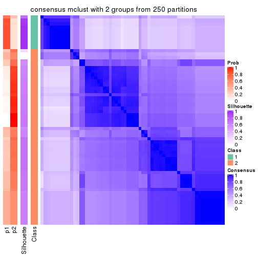
consensus_heatmap(res, k = 3)
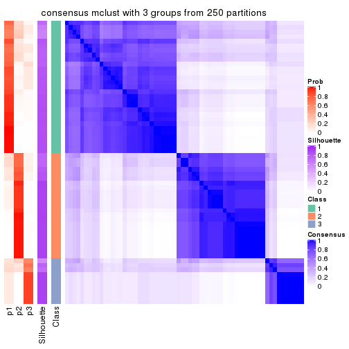
consensus_heatmap(res, k = 4)
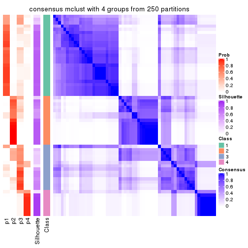
consensus_heatmap(res, k = 5)
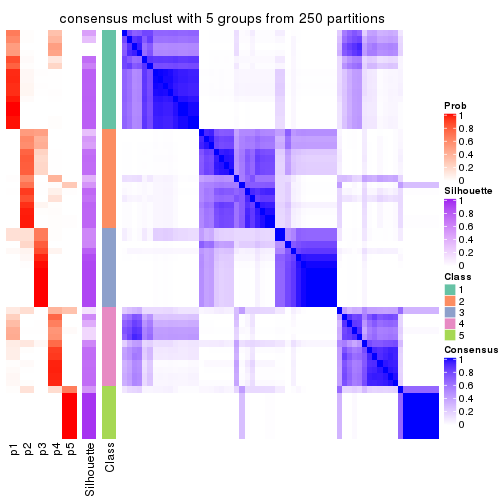
consensus_heatmap(res, k = 6)
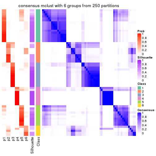
Heatmaps for the membership of samples in all partitions to see how consistent they are:
membership_heatmap(res, k = 2)
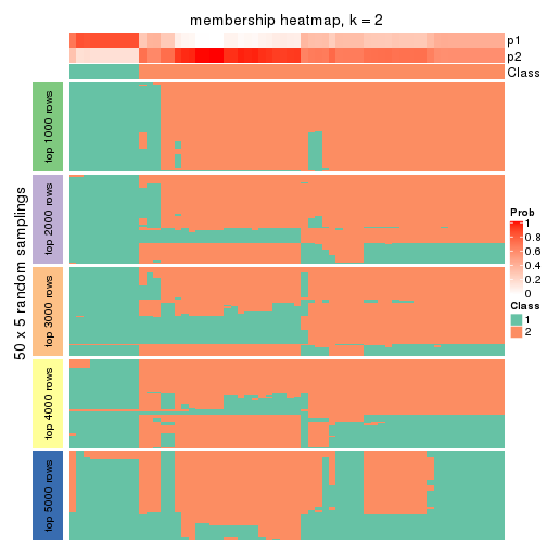
membership_heatmap(res, k = 3)
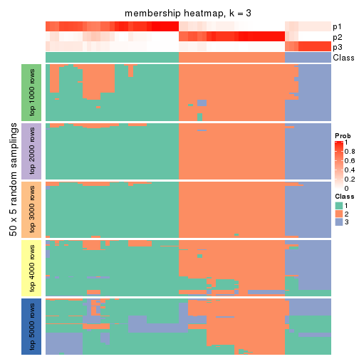
membership_heatmap(res, k = 4)
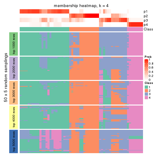
membership_heatmap(res, k = 5)
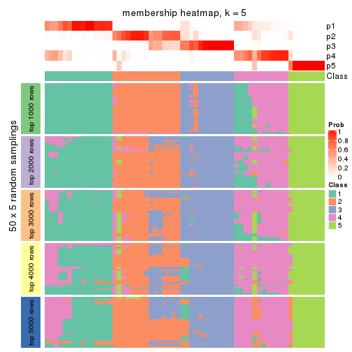
membership_heatmap(res, k = 6)
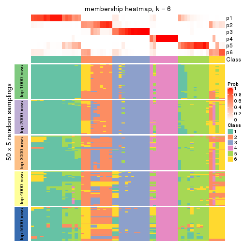
As soon as we have had the classes for columns, we can look for signatures which are significantly different between classes which can be candidate marks for certain classes. Following are the heatmaps for signatures.
Signature heatmaps where rows are scaled:
get_signatures(res, k = 2)
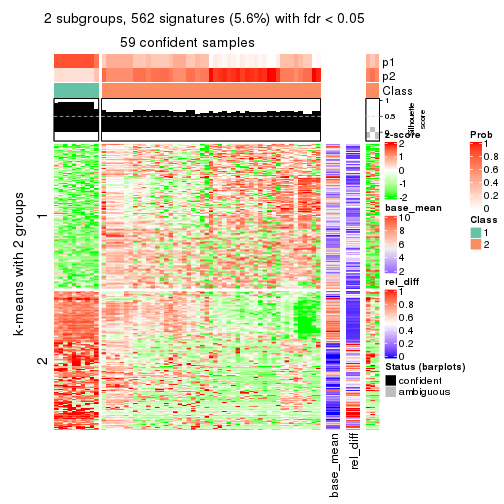
get_signatures(res, k = 3)
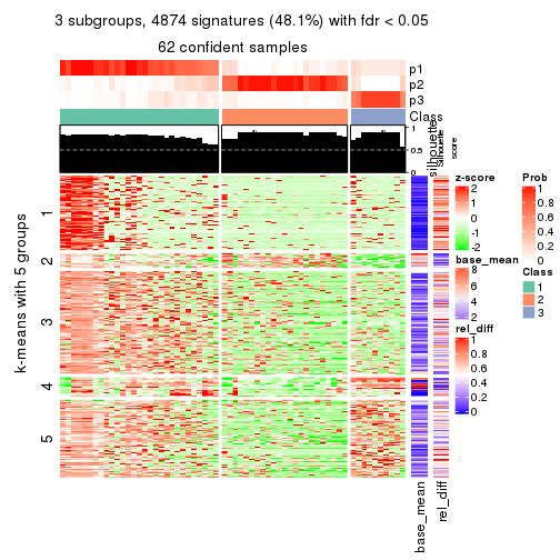
get_signatures(res, k = 4)
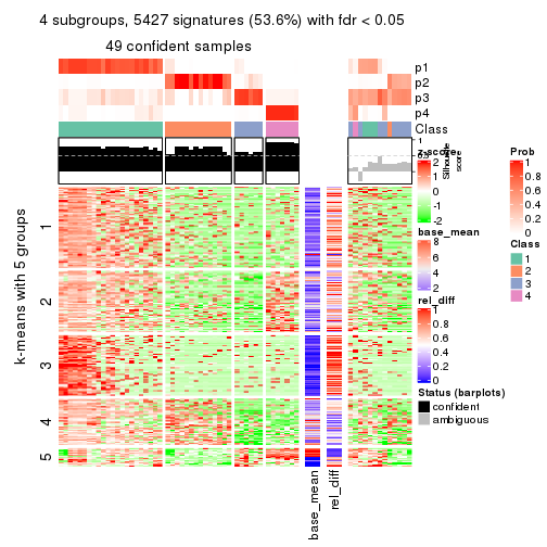
get_signatures(res, k = 5)
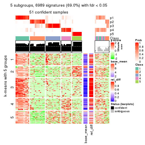
get_signatures(res, k = 6)
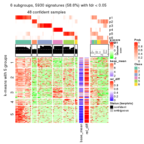
Signature heatmaps where rows are not scaled:
get_signatures(res, k = 2, scale_rows = FALSE)
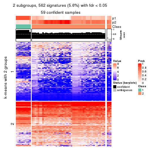
get_signatures(res, k = 3, scale_rows = FALSE)
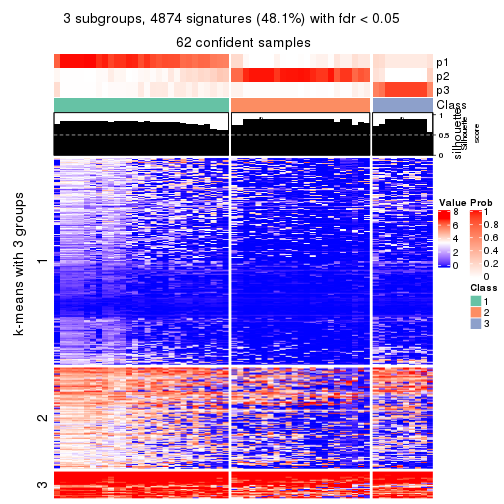
get_signatures(res, k = 4, scale_rows = FALSE)
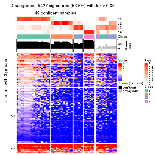
get_signatures(res, k = 5, scale_rows = FALSE)
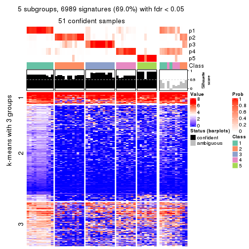
get_signatures(res, k = 6, scale_rows = FALSE)
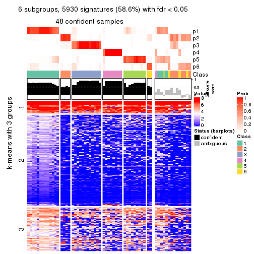
Compare the overlap of signatures from different k:
compare_signatures(res)
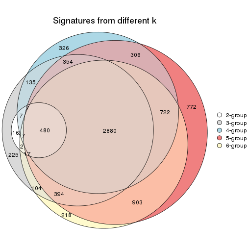
get_signature() returns a data frame invisibly. TO get the list of signatures, the function
call should be assigned to a variable explicitly. In following code, if plot argument is set
to FALSE, no heatmap is plotted while only the differential analysis is performed.
# code only for demonstration
tb = get_signature(res, k = ..., plot = FALSE)
An example of the output of tb is:
#>   which_row         fdr    mean_1    mean_2 scaled_mean_1 scaled_mean_2 km
#> 1        38 0.042760348  8.373488  9.131774    -0.5533452     0.5164555  1
#> 2        40 0.018707592  7.106213  8.469186    -0.6173731     0.5762149  1
#> 3        55 0.019134737 10.221463 11.207825    -0.6159697     0.5749050  1
#> 4        59 0.006059896  5.921854  7.869574    -0.6899429     0.6439467  1
#> 5        60 0.018055526  8.928898 10.211722    -0.6204761     0.5791110  1
#> 6        98 0.009384629 15.714769 14.887706     0.6635654    -0.6193277  2
...
The columns in tb are:
which_row: row indices corresponding to the input matrix.fdr: FDR for the differential test. mean_x: The mean value in group x.scaled_mean_x: The mean value in group x after rows are scaled.km: Row groups if k-means clustering is applied to rows.UMAP plot which shows how samples are separated.
dimension_reduction(res, k = 2, method = "UMAP")
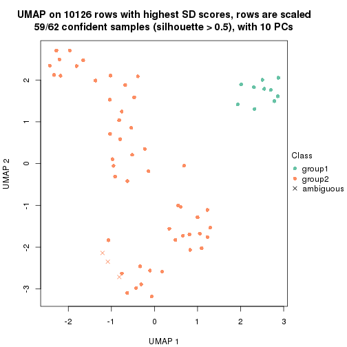
dimension_reduction(res, k = 3, method = "UMAP")
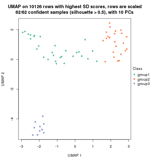
dimension_reduction(res, k = 4, method = "UMAP")
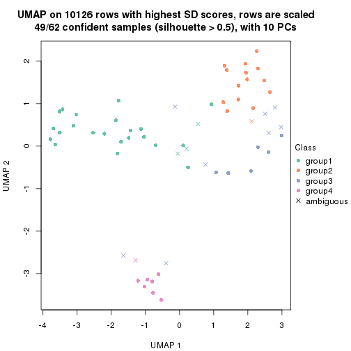
dimension_reduction(res, k = 5, method = "UMAP")
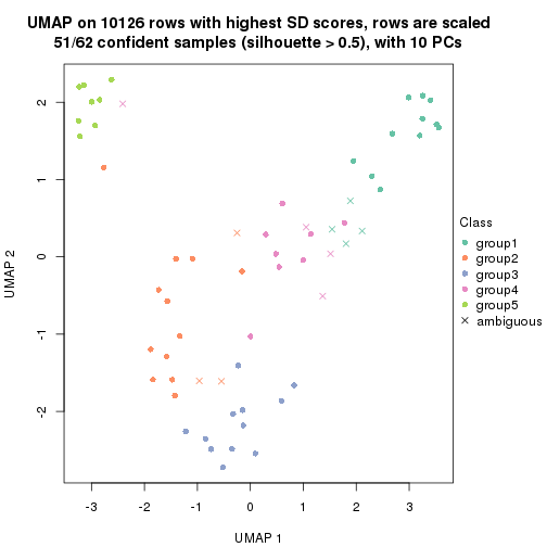
dimension_reduction(res, k = 6, method = "UMAP")
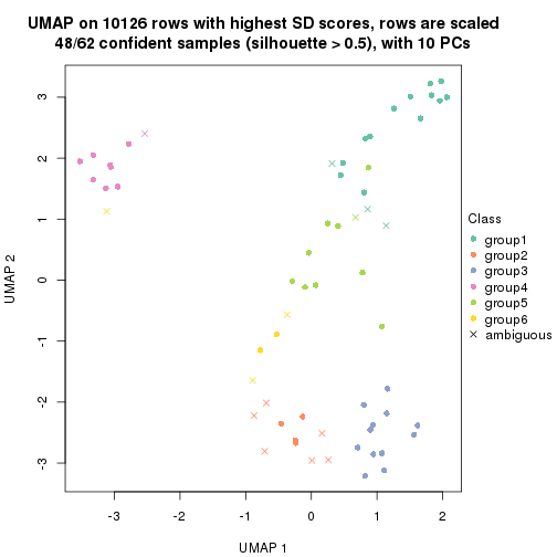
Following heatmap shows how subgroups are split when increasing k:
collect_classes(res)
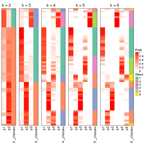
If matrix rows can be associated to genes, consider to use functional_enrichment(res,
...) to perform function enrichment for the signature genes. See this vignette for more detailed explanations.
The object with results only for a single top-value method and a single partition method can be extracted as:
res = res_list["SD", "NMF"]
# you can also extract it by
# res = res_list["SD:NMF"]
A summary of res and all the functions that can be applied to it:
res
#> A 'ConsensusPartition' object with k = 2, 3, 4, 5, 6.
#>   On a matrix with 10126 rows and 62 columns.
#>   Top rows (1000, 2000, 3000, 4000, 5000) are extracted by 'SD' method.
#>   Subgroups are detected by 'NMF' method.
#>   Performed in total 1250 partitions by row resampling.
#>   Best k for subgroups seems to be 2.
#>
#> Following methods can be applied to this 'ConsensusPartition' object:
#>  [1] "cola_report"             "collect_classes"         "collect_plots"
#>  [4] "collect_stats"           "colnames"                "compare_signatures"
#>  [7] "consensus_heatmap"       "dimension_reduction"     "functional_enrichment"
#> [10] "get_anno_col"            "get_anno"                "get_classes"
#> [13] "get_consensus"           "get_matrix"              "get_membership"
#> [16] "get_param"               "get_signatures"          "get_stats"
#> [19] "is_best_k"               "is_stable_k"             "membership_heatmap"
#> [22] "ncol"                    "nrow"                    "plot_ecdf"
#> [25] "rownames"                "select_partition_number" "show"
#> [28] "suggest_best_k"          "test_to_known_factors"
collect_plots() function collects all the plots made from res for all k (number of partitions)
into one single page to provide an easy and fast comparison between different k.
collect_plots(res)
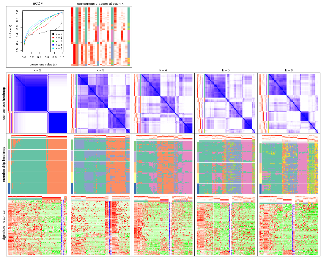
The plots are:
k and the heatmap of
predicted classes for each k.k.k.k.All the plots in panels can be made by individual functions and they are plotted later in this section.
select_partition_number() produces several plots showing different
statistics for choosing “optimized” k. There are following statistics:
k;k, the area increased is defined as \(A_k - A_{k-1}\).The detailed explanations of these statistics can be found in the cola vignette.
Generally speaking, lower PAC score, higher mean silhouette score or higher
concordance corresponds to better partition. Rand index and Jaccard index
measure how similar the current partition is compared to partition with k-1.
If they are too similar, we won't accept k is better than k-1.
select_partition_number(res)
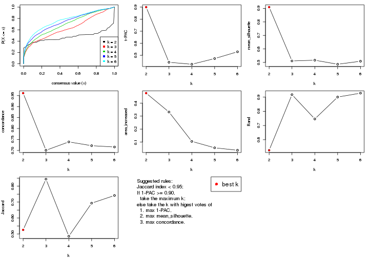
The numeric values for all these statistics can be obtained by get_stats().
get_stats(res)
#>   k 1-PAC mean_silhouette concordance area_increased  Rand Jaccard
#> 2 2 0.900           0.910       0.961         0.4771 0.526   0.526
#> 3 3 0.442           0.511       0.701         0.3317 0.918   0.844
#> 4 4 0.426           0.516       0.739         0.1051 0.746   0.486
#> 5 5 0.473           0.486       0.722         0.0557 0.901   0.693
#> 6 6 0.529           0.509       0.716         0.0369 0.928   0.741
suggest_best_k() suggests the best \(k\) based on these statistics. The rules are as follows:
suggest_best_k(res)
#> [1] 2
Following shows the table of the partitions (You need to click the show/hide
code output link to see it). The membership matrix (columns with name p*)
is inferred by
clue::cl_consensus()
function with the SE method. Basically the value in the membership matrix
represents the probability to belong to a certain group. The finall class
label for an item is determined with the group with highest probability it
belongs to.
In get_classes() function, the entropy is calculated from the membership
matrix and the silhouette score is calculated from the consensus matrix.
cbind(get_classes(res, k = 2), get_membership(res, k = 2))
#>            class entropy silhouette    p1    p2
#> SRR764776      1  0.0000     0.9581 1.000 0.000
#> SRR764777      1  0.0000     0.9581 1.000 0.000
#> SRR764778      1  0.0000     0.9581 1.000 0.000
#> SRR764779      1  0.0000     0.9581 1.000 0.000
#> SRR764780      1  0.0000     0.9581 1.000 0.000
#> SRR764781      1  0.0000     0.9581 1.000 0.000
#> SRR764782      1  0.0000     0.9581 1.000 0.000
#> SRR764783      1  0.1633     0.9471 0.976 0.024
#> SRR764784      1  0.0000     0.9581 1.000 0.000
#> SRR764785      1  0.2603     0.9366 0.956 0.044
#> SRR764786      1  0.0000     0.9581 1.000 0.000
#> SRR764787      1  0.2423     0.9383 0.960 0.040
#> SRR764788      1  0.3114     0.9277 0.944 0.056
#> SRR764789      1  0.0000     0.9581 1.000 0.000
#> SRR764790      1  0.0000     0.9581 1.000 0.000
#> SRR764791      1  0.6148     0.8356 0.848 0.152
#> SRR764792      1  0.4161     0.9053 0.916 0.084
#> SRR764793      1  0.3733     0.9157 0.928 0.072
#> SRR764794      1  0.0000     0.9581 1.000 0.000
#> SRR764795      1  0.0000     0.9581 1.000 0.000
#> SRR764796      1  0.0000     0.9581 1.000 0.000
#> SRR764797      1  0.4161     0.9059 0.916 0.084
#> SRR764798      2  0.0000     0.9579 0.000 1.000
#> SRR764799      2  0.9944     0.0788 0.456 0.544
#> SRR764800      1  0.1184     0.9511 0.984 0.016
#> SRR764801      2  0.0000     0.9579 0.000 1.000
#> SRR764802      1  0.0000     0.9581 1.000 0.000
#> SRR764803      1  0.0000     0.9581 1.000 0.000
#> SRR764804      2  0.0000     0.9579 0.000 1.000
#> SRR764805      2  0.0000     0.9579 0.000 1.000
#> SRR764806      2  0.0000     0.9579 0.000 1.000
#> SRR764807      2  0.0000     0.9579 0.000 1.000
#> SRR764808      2  0.9795     0.2962 0.416 0.584
#> SRR764809      2  0.0000     0.9579 0.000 1.000
#> SRR764810      2  0.0000     0.9579 0.000 1.000
#> SRR764811      2  0.0000     0.9579 0.000 1.000
#> SRR764812      2  0.0000     0.9579 0.000 1.000
#> SRR764813      2  0.0000     0.9579 0.000 1.000
#> SRR764814      1  0.7674     0.7379 0.776 0.224
#> SRR764815      1  0.6048     0.8197 0.852 0.148
#> SRR764816      1  0.9710     0.3706 0.600 0.400
#> SRR764817      1  0.6801     0.8012 0.820 0.180
#> SRR1066622     1  0.0000     0.9581 1.000 0.000
#> SRR1066623     1  0.0000     0.9581 1.000 0.000
#> SRR1066624     1  0.0000     0.9581 1.000 0.000
#> SRR1066625     1  0.0000     0.9581 1.000 0.000
#> SRR1066626     1  0.0000     0.9581 1.000 0.000
#> SRR1066627     1  0.0000     0.9581 1.000 0.000
#> SRR1066628     1  0.0000     0.9581 1.000 0.000
#> SRR1066629     1  0.0000     0.9581 1.000 0.000
#> SRR1066630     1  0.0672     0.9541 0.992 0.008
#> SRR1066631     1  0.0000     0.9581 1.000 0.000
#> SRR1066632     2  0.0000     0.9579 0.000 1.000
#> SRR1066633     2  0.0000     0.9579 0.000 1.000
#> SRR1066634     2  0.0000     0.9579 0.000 1.000
#> SRR1066635     2  0.0000     0.9579 0.000 1.000
#> SRR1066636     2  0.0000     0.9579 0.000 1.000
#> SRR1066637     2  0.0000     0.9579 0.000 1.000
#> SRR1066638     2  0.0000     0.9579 0.000 1.000
#> SRR1066639     2  0.0000     0.9579 0.000 1.000
#> SRR1066640     2  0.0000     0.9579 0.000 1.000
#> SRR1066641     2  0.0000     0.9579 0.000 1.000
cbind(get_classes(res, k = 3), get_membership(res, k = 3))
#>            class entropy silhouette    p1    p2    p3
#> SRR764776      1  0.6796     0.0485 0.612 0.020 0.368
#> SRR764777      1  0.6339     0.1077 0.632 0.008 0.360
#> SRR764778      1  0.5835     0.1677 0.660 0.000 0.340
#> SRR764779      1  0.5859     0.1599 0.656 0.000 0.344
#> SRR764780      1  0.5650     0.2290 0.688 0.000 0.312
#> SRR764781      1  0.2878     0.5171 0.904 0.000 0.096
#> SRR764782      1  0.1878     0.5426 0.952 0.004 0.044
#> SRR764783      1  0.6935     0.0464 0.604 0.024 0.372
#> SRR764784      1  0.0592     0.5570 0.988 0.000 0.012
#> SRR764785      1  0.7465     0.3980 0.656 0.072 0.272
#> SRR764786      1  0.6297     0.4764 0.640 0.008 0.352
#> SRR764787      1  0.5521     0.4180 0.788 0.032 0.180
#> SRR764788      1  0.6843     0.1363 0.640 0.028 0.332
#> SRR764789      1  0.3412     0.5631 0.876 0.000 0.124
#> SRR764790      1  0.6617     0.4240 0.556 0.008 0.436
#> SRR764791      1  0.6291     0.3674 0.768 0.080 0.152
#> SRR764792      1  0.7937    -0.1383 0.568 0.068 0.364
#> SRR764793      1  0.5470     0.4208 0.796 0.036 0.168
#> SRR764794      1  0.5200     0.5316 0.796 0.020 0.184
#> SRR764795      1  0.0592     0.5598 0.988 0.000 0.012
#> SRR764796      1  0.2066     0.5643 0.940 0.000 0.060
#> SRR764797      1  0.7114    -0.0305 0.584 0.028 0.388
#> SRR764798      2  0.5785     0.5268 0.004 0.696 0.300
#> SRR764799      3  0.9808     0.5760 0.264 0.308 0.428
#> SRR764800      1  0.7156    -0.0853 0.572 0.028 0.400
#> SRR764801      2  0.5728     0.5892 0.008 0.720 0.272
#> SRR764802      1  0.2878     0.5172 0.904 0.000 0.096
#> SRR764803      1  0.1163     0.5621 0.972 0.000 0.028
#> SRR764804      2  0.2448     0.8387 0.000 0.924 0.076
#> SRR764805      2  0.1860     0.8383 0.000 0.948 0.052
#> SRR764806      2  0.2200     0.8459 0.004 0.940 0.056
#> SRR764807      2  0.6357     0.6455 0.020 0.684 0.296
#> SRR764808      3  0.8790    -0.1644 0.128 0.340 0.532
#> SRR764809      2  0.1399     0.8405 0.004 0.968 0.028
#> SRR764810      2  0.2796     0.8220 0.000 0.908 0.092
#> SRR764811      2  0.3686     0.7882 0.000 0.860 0.140
#> SRR764812      2  0.1860     0.8376 0.000 0.948 0.052
#> SRR764813      2  0.6379     0.6826 0.032 0.712 0.256
#> SRR764814      3  0.9421     0.5407 0.388 0.176 0.436
#> SRR764815      1  0.7909     0.1660 0.648 0.240 0.112
#> SRR764816      3  0.9724     0.5997 0.328 0.236 0.436
#> SRR764817      3  0.9252     0.5162 0.396 0.156 0.448
#> SRR1066622     1  0.5706     0.5174 0.680 0.000 0.320
#> SRR1066623     1  0.5785     0.5114 0.668 0.000 0.332
#> SRR1066624     1  0.5058     0.5366 0.756 0.000 0.244
#> SRR1066625     1  0.5591     0.5224 0.696 0.000 0.304
#> SRR1066626     1  0.5835     0.5063 0.660 0.000 0.340
#> SRR1066627     1  0.5810     0.5085 0.664 0.000 0.336
#> SRR1066628     1  0.5706     0.5164 0.680 0.000 0.320
#> SRR1066629     1  0.5560     0.5239 0.700 0.000 0.300
#> SRR1066630     1  0.6735     0.4250 0.564 0.012 0.424
#> SRR1066631     1  0.5905     0.4983 0.648 0.000 0.352
#> SRR1066632     2  0.3043     0.8436 0.008 0.908 0.084
#> SRR1066633     2  0.4209     0.7999 0.016 0.856 0.128
#> SRR1066634     2  0.5581     0.7458 0.036 0.788 0.176
#> SRR1066635     2  0.2261     0.8443 0.000 0.932 0.068
#> SRR1066636     2  0.3771     0.8125 0.012 0.876 0.112
#> SRR1066637     2  0.5355     0.7477 0.032 0.800 0.168
#> SRR1066638     2  0.3120     0.8409 0.012 0.908 0.080
#> SRR1066639     2  0.2866     0.8453 0.008 0.916 0.076
#> SRR1066640     2  0.2749     0.8390 0.012 0.924 0.064
#> SRR1066641     2  0.5070     0.7445 0.004 0.772 0.224
cbind(get_classes(res, k = 4), get_membership(res, k = 4))
#>            class entropy silhouette    p1    p2    p3    p4
#> SRR764776      1   0.238     0.7309 0.924 0.024 0.004 0.048
#> SRR764777      1   0.210     0.7360 0.928 0.012 0.000 0.060
#> SRR764778      1   0.286     0.7271 0.888 0.004 0.008 0.100
#> SRR764779      1   0.280     0.7281 0.892 0.004 0.008 0.096
#> SRR764780      1   0.298     0.7167 0.872 0.000 0.008 0.120
#> SRR764781      1   0.474     0.4927 0.668 0.000 0.004 0.328
#> SRR764782      1   0.603     0.2886 0.564 0.000 0.048 0.388
#> SRR764783      1   0.223     0.7372 0.924 0.008 0.004 0.064
#> SRR764784      1   0.559     0.0154 0.492 0.008 0.008 0.492
#> SRR764785      3   0.774    -0.1976 0.412 0.012 0.420 0.156
#> SRR764786      4   0.742     0.2201 0.184 0.000 0.332 0.484
#> SRR764787      1   0.741     0.4048 0.560 0.012 0.168 0.260
#> SRR764788      1   0.301     0.7262 0.888 0.000 0.032 0.080
#> SRR764789      4   0.716     0.1878 0.372 0.000 0.140 0.488
#> SRR764790      4   0.557     0.4432 0.044 0.008 0.248 0.700
#> SRR764791      1   0.677     0.5598 0.620 0.084 0.020 0.276
#> SRR764792      1   0.458     0.7015 0.832 0.044 0.056 0.068
#> SRR764793      1   0.569     0.5581 0.676 0.024 0.020 0.280
#> SRR764794      1   0.820     0.2788 0.452 0.020 0.292 0.236
#> SRR764795      4   0.565     0.1359 0.432 0.000 0.024 0.544
#> SRR764796      4   0.505     0.3577 0.356 0.004 0.004 0.636
#> SRR764797      1   0.177     0.7286 0.948 0.004 0.012 0.036
#> SRR764798      2   0.640     0.3376 0.408 0.524 0.068 0.000
#> SRR764799      1   0.422     0.5105 0.792 0.184 0.024 0.000
#> SRR764800      1   0.283     0.7254 0.908 0.036 0.008 0.048
#> SRR764801      2   0.606     0.4004 0.400 0.552 0.048 0.000
#> SRR764802      1   0.498     0.4816 0.652 0.004 0.004 0.340
#> SRR764803      4   0.577     0.0106 0.464 0.000 0.028 0.508
#> SRR764804      2   0.389     0.5978 0.012 0.804 0.184 0.000
#> SRR764805      2   0.423     0.5438 0.008 0.776 0.212 0.004
#> SRR764806      2   0.388     0.6230 0.048 0.840 0.112 0.000
#> SRR764807      3   0.749     0.2394 0.080 0.316 0.556 0.048
#> SRR764808      3   0.774     0.3124 0.020 0.140 0.480 0.360
#> SRR764809      2   0.286     0.6101 0.008 0.880 0.112 0.000
#> SRR764810      2   0.483     0.4338 0.004 0.680 0.312 0.004
#> SRR764811      2   0.629    -0.0129 0.020 0.508 0.448 0.024
#> SRR764812      2   0.427     0.5914 0.020 0.804 0.168 0.008
#> SRR764813      3   0.698     0.1533 0.044 0.352 0.560 0.044
#> SRR764814      1   0.251     0.6745 0.916 0.064 0.008 0.012
#> SRR764815      1   0.888     0.2917 0.452 0.072 0.232 0.244
#> SRR764816      1   0.361     0.6147 0.852 0.124 0.016 0.008
#> SRR764817      1   0.344     0.6572 0.872 0.096 0.016 0.016
#> SRR1066622     4   0.179     0.7573 0.068 0.000 0.000 0.932
#> SRR1066623     4   0.172     0.7566 0.064 0.000 0.000 0.936
#> SRR1066624     4   0.247     0.7438 0.108 0.000 0.000 0.892
#> SRR1066625     4   0.179     0.7568 0.068 0.000 0.000 0.932
#> SRR1066626     4   0.172     0.7560 0.064 0.000 0.000 0.936
#> SRR1066627     4   0.147     0.7490 0.052 0.000 0.000 0.948
#> SRR1066628     4   0.172     0.7564 0.064 0.000 0.000 0.936
#> SRR1066629     4   0.208     0.7541 0.084 0.000 0.000 0.916
#> SRR1066630     4   0.205     0.6315 0.004 0.000 0.072 0.924
#> SRR1066631     4   0.145     0.7297 0.036 0.000 0.008 0.956
#> SRR1066632     2   0.441     0.6474 0.108 0.812 0.080 0.000
#> SRR1066633     2   0.522     0.6169 0.200 0.736 0.064 0.000
#> SRR1066634     2   0.594     0.4790 0.324 0.620 0.056 0.000
#> SRR1066635     2   0.398     0.6039 0.040 0.828 0.132 0.000
#> SRR1066636     2   0.436     0.6526 0.148 0.804 0.048 0.000
#> SRR1066637     2   0.533     0.5946 0.220 0.720 0.060 0.000
#> SRR1066638     2   0.606     0.5680 0.136 0.684 0.180 0.000
#> SRR1066639     2   0.384     0.6621 0.092 0.852 0.052 0.004
#> SRR1066640     2   0.437     0.6505 0.120 0.812 0.068 0.000
#> SRR1066641     3   0.610     0.0769 0.020 0.396 0.564 0.020
cbind(get_classes(res, k = 5), get_membership(res, k = 5))
#>            class entropy silhouette    p1    p2    p3    p4    p5
#> SRR764776      1   0.130     0.6786 0.956 0.000 0.028 0.016 0.000
#> SRR764777      1   0.112     0.6816 0.964 0.000 0.016 0.020 0.000
#> SRR764778      1   0.156     0.6871 0.940 0.000 0.008 0.052 0.000
#> SRR764779      1   0.156     0.6871 0.940 0.000 0.008 0.052 0.000
#> SRR764780      1   0.185     0.6835 0.912 0.000 0.000 0.088 0.000
#> SRR764781      1   0.346     0.6249 0.772 0.004 0.000 0.224 0.000
#> SRR764782      1   0.526     0.5215 0.648 0.088 0.000 0.264 0.000
#> SRR764783      1   0.172     0.6896 0.936 0.004 0.008 0.052 0.000
#> SRR764784      1   0.508     0.4311 0.576 0.032 0.004 0.388 0.000
#> SRR764785      2   0.597     0.3609 0.336 0.580 0.004 0.044 0.036
#> SRR764786      2   0.642     0.4213 0.208 0.564 0.000 0.216 0.012
#> SRR764787      1   0.626     0.2227 0.536 0.304 0.004 0.156 0.000
#> SRR764788      1   0.296     0.6687 0.876 0.060 0.004 0.060 0.000
#> SRR764789      1   0.670     0.0468 0.408 0.248 0.000 0.344 0.000
#> SRR764790      4   0.695     0.0249 0.028 0.372 0.036 0.496 0.068
#> SRR764791      1   0.650     0.5144 0.608 0.032 0.156 0.200 0.004
#> SRR764792      1   0.437     0.5928 0.792 0.112 0.076 0.020 0.000
#> SRR764793      1   0.517     0.6132 0.720 0.036 0.056 0.188 0.000
#> SRR764794      2   0.676     0.1052 0.420 0.444 0.032 0.100 0.004
#> SRR764795      1   0.509     0.2954 0.524 0.036 0.000 0.440 0.000
#> SRR764796      4   0.478     0.2182 0.364 0.000 0.020 0.612 0.004
#> SRR764797      1   0.172     0.6822 0.944 0.020 0.016 0.020 0.000
#> SRR764798      3   0.586     0.3447 0.356 0.008 0.552 0.000 0.084
#> SRR764799      1   0.372     0.5064 0.776 0.004 0.208 0.000 0.012
#> SRR764800      1   0.174     0.6665 0.932 0.000 0.056 0.012 0.000
#> SRR764801      3   0.607     0.4266 0.272 0.036 0.612 0.000 0.080
#> SRR764802      1   0.352     0.6236 0.764 0.004 0.000 0.232 0.000
#> SRR764803      1   0.508     0.4695 0.604 0.048 0.000 0.348 0.000
#> SRR764804      3   0.514     0.3992 0.012 0.128 0.720 0.000 0.140
#> SRR764805      3   0.630     0.0299 0.000 0.140 0.532 0.008 0.320
#> SRR764806      3   0.619     0.2586 0.036 0.060 0.572 0.004 0.328
#> SRR764807      5   0.757     0.3623 0.008 0.376 0.168 0.048 0.400
#> SRR764808      2   0.823    -0.1754 0.004 0.392 0.112 0.240 0.252
#> SRR764809      3   0.563     0.2045 0.000 0.108 0.600 0.000 0.292
#> SRR764810      5   0.666     0.2217 0.004 0.196 0.364 0.000 0.436
#> SRR764811      5   0.512     0.4936 0.016 0.060 0.228 0.000 0.696
#> SRR764812      3   0.462     0.4294 0.008 0.136 0.760 0.000 0.096
#> SRR764813      2   0.732    -0.3453 0.028 0.516 0.144 0.028 0.284
#> SRR764814      1   0.235     0.6376 0.904 0.008 0.076 0.000 0.012
#> SRR764815      1   0.707    -0.1900 0.444 0.408 0.072 0.068 0.008
#> SRR764816      1   0.344     0.5460 0.808 0.004 0.176 0.000 0.012
#> SRR764817      1   0.300     0.5767 0.840 0.000 0.148 0.000 0.012
#> SRR1066622     4   0.183     0.8364 0.076 0.004 0.000 0.920 0.000
#> SRR1066623     4   0.170     0.8427 0.068 0.000 0.000 0.928 0.004
#> SRR1066624     4   0.250     0.8038 0.112 0.004 0.000 0.880 0.004
#> SRR1066625     4   0.173     0.8428 0.060 0.004 0.000 0.932 0.004
#> SRR1066626     4   0.166     0.8405 0.056 0.004 0.000 0.936 0.004
#> SRR1066627     4   0.159     0.8395 0.052 0.004 0.000 0.940 0.004
#> SRR1066628     4   0.141     0.8432 0.060 0.000 0.000 0.940 0.000
#> SRR1066629     4   0.185     0.8295 0.088 0.000 0.000 0.912 0.000
#> SRR1066630     4   0.380     0.6319 0.008 0.096 0.012 0.836 0.048
#> SRR1066631     4   0.133     0.8203 0.032 0.008 0.000 0.956 0.004
#> SRR1066632     3   0.385     0.5548 0.048 0.076 0.840 0.004 0.032
#> SRR1066633     3   0.456     0.5591 0.168 0.028 0.764 0.000 0.040
#> SRR1066634     3   0.521     0.5116 0.204 0.020 0.704 0.000 0.072
#> SRR1066635     3   0.531     0.2715 0.016 0.040 0.624 0.000 0.320
#> SRR1066636     3   0.417     0.5858 0.096 0.016 0.812 0.004 0.072
#> SRR1066637     3   0.402     0.5753 0.124 0.024 0.812 0.000 0.040
#> SRR1066638     3   0.635     0.4084 0.104 0.036 0.612 0.004 0.244
#> SRR1066639     3   0.367     0.5713 0.052 0.020 0.852 0.008 0.068
#> SRR1066640     3   0.491     0.5628 0.092 0.032 0.768 0.004 0.104
#> SRR1066641     5   0.574     0.4868 0.000 0.152 0.232 0.000 0.616
cbind(get_classes(res, k = 6), get_membership(res, k = 6))
#>            class entropy silhouette    p1    p2    p3    p4    p5    p6
#> SRR764776      1  0.1269     0.7445 0.956 0.000 0.020 0.012 0.012 0.000
#> SRR764777      1  0.1262     0.7484 0.956 0.000 0.016 0.020 0.008 0.000
#> SRR764778      1  0.1410     0.7514 0.944 0.000 0.004 0.044 0.008 0.000
#> SRR764779      1  0.1296     0.7517 0.948 0.000 0.004 0.044 0.004 0.000
#> SRR764780      1  0.1349     0.7508 0.940 0.000 0.000 0.056 0.004 0.000
#> SRR764781      1  0.3088     0.6866 0.808 0.000 0.000 0.172 0.020 0.000
#> SRR764782      1  0.4563     0.5742 0.700 0.000 0.000 0.164 0.136 0.000
#> SRR764783      1  0.1693     0.7459 0.932 0.000 0.000 0.044 0.020 0.004
#> SRR764784      1  0.4468     0.4911 0.640 0.000 0.004 0.316 0.040 0.000
#> SRR764785      5  0.4528     0.4979 0.228 0.028 0.016 0.016 0.712 0.000
#> SRR764786      5  0.4490     0.4229 0.136 0.008 0.012 0.068 0.764 0.012
#> SRR764787      5  0.5912     0.3605 0.404 0.008 0.016 0.088 0.480 0.004
#> SRR764788      1  0.3088     0.6829 0.832 0.000 0.000 0.048 0.120 0.000
#> SRR764789      5  0.5779     0.4933 0.304 0.004 0.000 0.180 0.512 0.000
#> SRR764790      5  0.7715     0.0899 0.044 0.040 0.044 0.328 0.428 0.116
#> SRR764791      1  0.6276     0.5476 0.632 0.012 0.164 0.116 0.060 0.016
#> SRR764792      1  0.4483     0.5674 0.728 0.000 0.068 0.004 0.188 0.012
#> SRR764793      1  0.5297     0.6217 0.692 0.000 0.104 0.128 0.076 0.000
#> SRR764794      5  0.6245     0.4641 0.368 0.004 0.032 0.044 0.508 0.044
#> SRR764795      1  0.4868     0.4026 0.592 0.000 0.000 0.332 0.076 0.000
#> SRR764796      4  0.4700    -0.1299 0.456 0.004 0.012 0.512 0.016 0.000
#> SRR764797      1  0.1759     0.7240 0.924 0.000 0.004 0.004 0.064 0.004
#> SRR764798      3  0.6428     0.3596 0.348 0.048 0.488 0.000 0.012 0.104
#> SRR764799      1  0.4113     0.5777 0.764 0.020 0.180 0.000 0.020 0.016
#> SRR764800      1  0.1657     0.7368 0.936 0.000 0.040 0.012 0.012 0.000
#> SRR764801      3  0.6777     0.3504 0.324 0.044 0.452 0.000 0.012 0.168
#> SRR764802      1  0.3312     0.6818 0.792 0.000 0.000 0.180 0.028 0.000
#> SRR764803      1  0.4473     0.5553 0.676 0.000 0.000 0.252 0.072 0.000
#> SRR764804      3  0.5601    -0.0162 0.004 0.064 0.552 0.000 0.032 0.348
#> SRR764805      6  0.6064     0.3261 0.000 0.128 0.280 0.000 0.044 0.548
#> SRR764806      3  0.7094    -0.2081 0.036 0.200 0.416 0.000 0.028 0.320
#> SRR764807      2  0.7639     0.2526 0.012 0.440 0.132 0.008 0.208 0.200
#> SRR764808      5  0.8535    -0.2906 0.004 0.124 0.096 0.168 0.312 0.296
#> SRR764809      6  0.6145     0.2609 0.000 0.192 0.368 0.000 0.012 0.428
#> SRR764810      6  0.6080     0.1859 0.000 0.228 0.188 0.000 0.032 0.552
#> SRR764811      2  0.5322     0.2700 0.012 0.704 0.120 0.000 0.052 0.112
#> SRR764812      3  0.5737     0.1777 0.012 0.080 0.652 0.008 0.040 0.208
#> SRR764813      6  0.7431    -0.0565 0.020 0.184 0.104 0.000 0.248 0.444
#> SRR764814      1  0.2581     0.7139 0.900 0.012 0.036 0.004 0.036 0.012
#> SRR764815      5  0.6260     0.4553 0.356 0.024 0.060 0.016 0.520 0.024
#> SRR764816      1  0.3944     0.6012 0.784 0.020 0.160 0.000 0.020 0.016
#> SRR764817      1  0.3353     0.6428 0.824 0.008 0.136 0.000 0.020 0.012
#> SRR1066622     4  0.1124     0.8772 0.036 0.000 0.000 0.956 0.008 0.000
#> SRR1066623     4  0.0972     0.8798 0.028 0.000 0.000 0.964 0.008 0.000
#> SRR1066624     4  0.1196     0.8741 0.040 0.000 0.000 0.952 0.008 0.000
#> SRR1066625     4  0.0692     0.8777 0.020 0.004 0.000 0.976 0.000 0.000
#> SRR1066626     4  0.1180     0.8769 0.024 0.008 0.000 0.960 0.004 0.004
#> SRR1066627     4  0.0603     0.8759 0.016 0.004 0.000 0.980 0.000 0.000
#> SRR1066628     4  0.0972     0.8803 0.028 0.000 0.000 0.964 0.008 0.000
#> SRR1066629     4  0.1542     0.8601 0.052 0.004 0.000 0.936 0.008 0.000
#> SRR1066630     4  0.3758     0.6736 0.000 0.056 0.016 0.828 0.072 0.028
#> SRR1066631     4  0.0696     0.8624 0.008 0.004 0.000 0.980 0.004 0.004
#> SRR1066632     3  0.4543     0.4469 0.056 0.032 0.772 0.004 0.016 0.120
#> SRR1066633     3  0.4791     0.5487 0.148 0.044 0.744 0.000 0.040 0.024
#> SRR1066634     3  0.5362     0.5004 0.212 0.044 0.676 0.000 0.032 0.036
#> SRR1066635     3  0.7060     0.0248 0.024 0.228 0.488 0.004 0.044 0.212
#> SRR1066636     3  0.4877     0.5454 0.108 0.052 0.752 0.000 0.024 0.064
#> SRR1066637     3  0.4200     0.5469 0.104 0.024 0.800 0.004 0.024 0.044
#> SRR1066638     3  0.6240     0.4307 0.096 0.216 0.600 0.000 0.016 0.072
#> SRR1066639     3  0.3648     0.5413 0.076 0.032 0.836 0.000 0.020 0.036
#> SRR1066640     3  0.5383     0.5176 0.116 0.084 0.708 0.000 0.016 0.076
#> SRR1066641     2  0.5958     0.3424 0.008 0.636 0.172 0.000 0.100 0.084
Heatmaps for the consensus matrix. It visualizes the probability of two samples to be in a same group.
consensus_heatmap(res, k = 2)
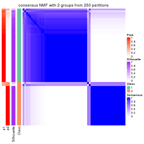
consensus_heatmap(res, k = 3)
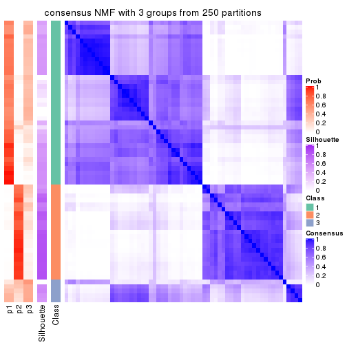
consensus_heatmap(res, k = 4)
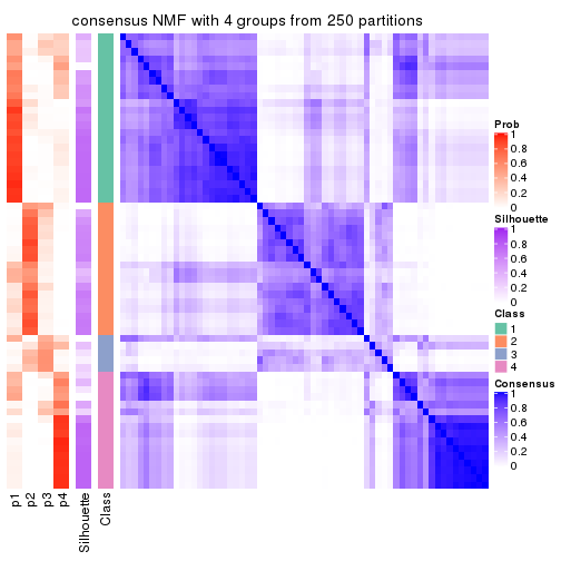
consensus_heatmap(res, k = 5)
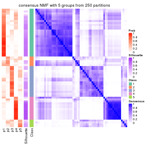
consensus_heatmap(res, k = 6)
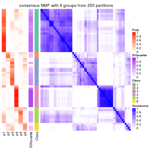
Heatmaps for the membership of samples in all partitions to see how consistent they are:
membership_heatmap(res, k = 2)
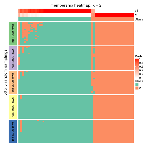
membership_heatmap(res, k = 3)
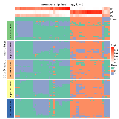
membership_heatmap(res, k = 4)
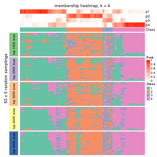
membership_heatmap(res, k = 5)
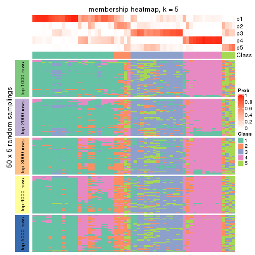
membership_heatmap(res, k = 6)
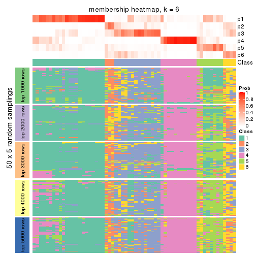
As soon as we have had the classes for columns, we can look for signatures which are significantly different between classes which can be candidate marks for certain classes. Following are the heatmaps for signatures.
Signature heatmaps where rows are scaled:
get_signatures(res, k = 2)
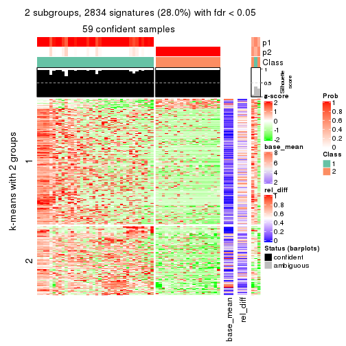
get_signatures(res, k = 3)
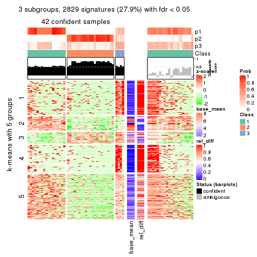
get_signatures(res, k = 4)
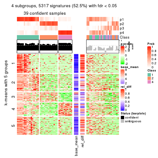
get_signatures(res, k = 5)
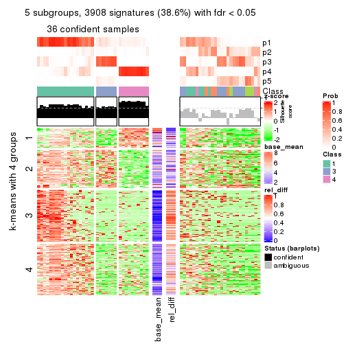
get_signatures(res, k = 6)
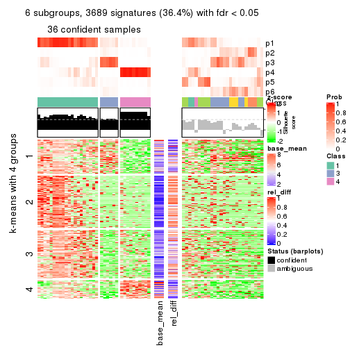
Signature heatmaps where rows are not scaled:
get_signatures(res, k = 2, scale_rows = FALSE)
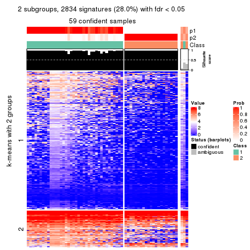
get_signatures(res, k = 3, scale_rows = FALSE)
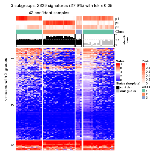
get_signatures(res, k = 4, scale_rows = FALSE)
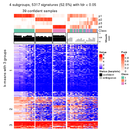
get_signatures(res, k = 5, scale_rows = FALSE)
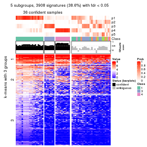
get_signatures(res, k = 6, scale_rows = FALSE)
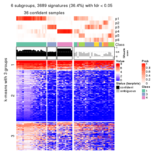
Compare the overlap of signatures from different k:
compare_signatures(res)
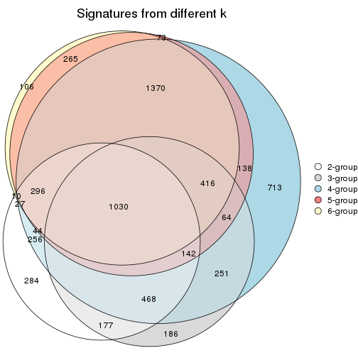
get_signature() returns a data frame invisibly. TO get the list of signatures, the function
call should be assigned to a variable explicitly. In following code, if plot argument is set
to FALSE, no heatmap is plotted while only the differential analysis is performed.
# code only for demonstration
tb = get_signature(res, k = ..., plot = FALSE)
An example of the output of tb is:
#>   which_row         fdr    mean_1    mean_2 scaled_mean_1 scaled_mean_2 km
#> 1        38 0.042760348  8.373488  9.131774    -0.5533452     0.5164555  1
#> 2        40 0.018707592  7.106213  8.469186    -0.6173731     0.5762149  1
#> 3        55 0.019134737 10.221463 11.207825    -0.6159697     0.5749050  1
#> 4        59 0.006059896  5.921854  7.869574    -0.6899429     0.6439467  1
#> 5        60 0.018055526  8.928898 10.211722    -0.6204761     0.5791110  1
#> 6        98 0.009384629 15.714769 14.887706     0.6635654    -0.6193277  2
...
The columns in tb are:
which_row: row indices corresponding to the input matrix.fdr: FDR for the differential test. mean_x: The mean value in group x.scaled_mean_x: The mean value in group x after rows are scaled.km: Row groups if k-means clustering is applied to rows.UMAP plot which shows how samples are separated.
dimension_reduction(res, k = 2, method = "UMAP")
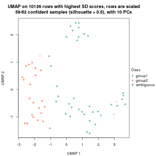
dimension_reduction(res, k = 3, method = "UMAP")
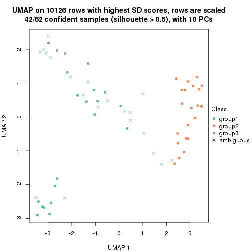
dimension_reduction(res, k = 4, method = "UMAP")
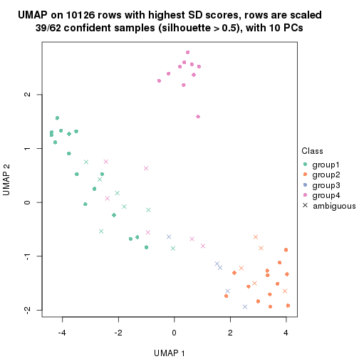
dimension_reduction(res, k = 5, method = "UMAP")
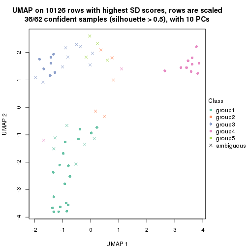
dimension_reduction(res, k = 6, method = "UMAP")
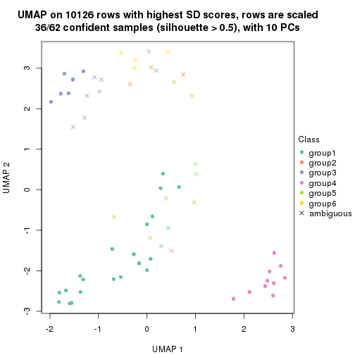
Following heatmap shows how subgroups are split when increasing k:
collect_classes(res)
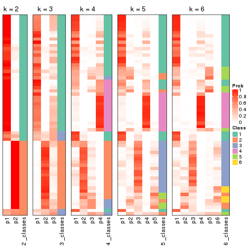
If matrix rows can be associated to genes, consider to use functional_enrichment(res,
...) to perform function enrichment for the signature genes. See this vignette for more detailed explanations.
The object with results only for a single top-value method and a single partition method can be extracted as:
res = res_list["CV", "hclust"]
# you can also extract it by
# res = res_list["CV:hclust"]
A summary of res and all the functions that can be applied to it:
res
#> A 'ConsensusPartition' object with k = 2, 3, 4, 5, 6.
#>   On a matrix with 10126 rows and 62 columns.
#>   Top rows (1000, 2000, 3000, 4000, 5000) are extracted by 'CV' method.
#>   Subgroups are detected by 'hclust' method.
#>   Performed in total 1250 partitions by row resampling.
#>   Best k for subgroups seems to be 3.
#>
#> Following methods can be applied to this 'ConsensusPartition' object:
#>  [1] "cola_report"             "collect_classes"         "collect_plots"
#>  [4] "collect_stats"           "colnames"                "compare_signatures"
#>  [7] "consensus_heatmap"       "dimension_reduction"     "functional_enrichment"
#> [10] "get_anno_col"            "get_anno"                "get_classes"
#> [13] "get_consensus"           "get_matrix"              "get_membership"
#> [16] "get_param"               "get_signatures"          "get_stats"
#> [19] "is_best_k"               "is_stable_k"             "membership_heatmap"
#> [22] "ncol"                    "nrow"                    "plot_ecdf"
#> [25] "rownames"                "select_partition_number" "show"
#> [28] "suggest_best_k"          "test_to_known_factors"
collect_plots() function collects all the plots made from res for all k (number of partitions)
into one single page to provide an easy and fast comparison between different k.
collect_plots(res)
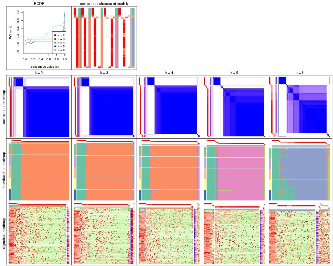
The plots are:
k and the heatmap of
predicted classes for each k.k.k.k.All the plots in panels can be made by individual functions and they are plotted later in this section.
select_partition_number() produces several plots showing different
statistics for choosing “optimized” k. There are following statistics:
k;k, the area increased is defined as \(A_k - A_{k-1}\).The detailed explanations of these statistics can be found in the cola vignette.
Generally speaking, lower PAC score, higher mean silhouette score or higher
concordance corresponds to better partition. Rand index and Jaccard index
measure how similar the current partition is compared to partition with k-1.
If they are too similar, we won't accept k is better than k-1.
select_partition_number(res)
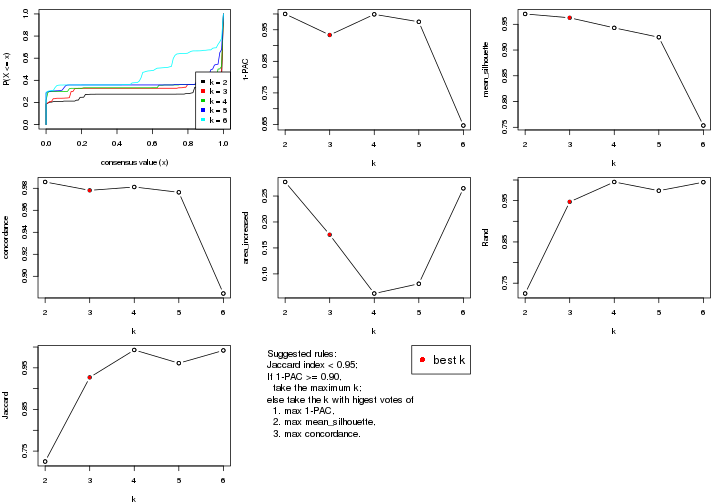
The numeric values for all these statistics can be obtained by get_stats().
get_stats(res)
#>   k 1-PAC mean_silhouette concordance area_increased  Rand Jaccard
#> 2 2 1.000           0.970       0.986         0.2771 0.725   0.725
#> 3 3 0.933           0.963       0.978         0.1754 0.947   0.927
#> 4 4 0.999           0.943       0.981         0.0622 0.995   0.993
#> 5 5 0.975           0.925       0.976         0.0810 0.974   0.961
#> 6 6 0.647           0.753       0.884         0.2648 0.995   0.992
suggest_best_k() suggests the best \(k\) based on these statistics. The rules are as follows:
suggest_best_k(res)
#> [1] 3
#> attr(,"optional")
#> [1] 2
There is also optional best \(k\) = 2 that is worth to check.
Following shows the table of the partitions (You need to click the show/hide
code output link to see it). The membership matrix (columns with name p*)
is inferred by
clue::cl_consensus()
function with the SE method. Basically the value in the membership matrix
represents the probability to belong to a certain group. The finall class
label for an item is determined with the group with highest probability it
belongs to.
In get_classes() function, the entropy is calculated from the membership
matrix and the silhouette score is calculated from the consensus matrix.
cbind(get_classes(res, k = 2), get_membership(res, k = 2))
#>            class entropy silhouette    p1    p2
#> SRR764776      1  0.0000      0.955 1.000 0.000
#> SRR764777      1  0.0000      0.955 1.000 0.000
#> SRR764778      1  0.0000      0.955 1.000 0.000
#> SRR764779      1  0.0000      0.955 1.000 0.000
#> SRR764780      2  0.0938      0.981 0.012 0.988
#> SRR764781      2  0.0938      0.981 0.012 0.988
#> SRR764782      2  0.0000      0.990 0.000 1.000
#> SRR764783      2  0.0376      0.987 0.004 0.996
#> SRR764784      2  0.0000      0.990 0.000 1.000
#> SRR764785      2  0.0000      0.990 0.000 1.000
#> SRR764786      2  0.0000      0.990 0.000 1.000
#> SRR764787      2  0.0000      0.990 0.000 1.000
#> SRR764788      2  0.0000      0.990 0.000 1.000
#> SRR764789      2  0.0000      0.990 0.000 1.000
#> SRR764790      2  0.0000      0.990 0.000 1.000
#> SRR764791      2  0.0000      0.990 0.000 1.000
#> SRR764792      2  0.0000      0.990 0.000 1.000
#> SRR764793      2  0.0000      0.990 0.000 1.000
#> SRR764794      2  0.0000      0.990 0.000 1.000
#> SRR764795      2  0.0000      0.990 0.000 1.000
#> SRR764796      2  0.0000      0.990 0.000 1.000
#> SRR764797      2  0.4431      0.898 0.092 0.908
#> SRR764798      2  0.6438      0.803 0.164 0.836
#> SRR764799      1  0.0000      0.955 1.000 0.000
#> SRR764800      1  0.0000      0.955 1.000 0.000
#> SRR764801      2  0.6438      0.803 0.164 0.836
#> SRR764802      2  0.0376      0.987 0.004 0.996
#> SRR764803      2  0.2043      0.962 0.032 0.968
#> SRR764804      2  0.0000      0.990 0.000 1.000
#> SRR764805      2  0.0000      0.990 0.000 1.000
#> SRR764806      2  0.0000      0.990 0.000 1.000
#> SRR764807      2  0.0000      0.990 0.000 1.000
#> SRR764808      2  0.0000      0.990 0.000 1.000
#> SRR764809      2  0.0000      0.990 0.000 1.000
#> SRR764810      2  0.0000      0.990 0.000 1.000
#> SRR764811      2  0.0000      0.990 0.000 1.000
#> SRR764812      2  0.0000      0.990 0.000 1.000
#> SRR764813      2  0.0000      0.990 0.000 1.000
#> SRR764814      1  0.7528      0.745 0.784 0.216
#> SRR764815      2  0.0000      0.990 0.000 1.000
#> SRR764816      1  0.0000      0.955 1.000 0.000
#> SRR764817      1  0.0000      0.955 1.000 0.000
#> SRR1066622     2  0.0000      0.990 0.000 1.000
#> SRR1066623     2  0.0000      0.990 0.000 1.000
#> SRR1066624     1  0.6887      0.791 0.816 0.184
#> SRR1066625     2  0.0000      0.990 0.000 1.000
#> SRR1066626     2  0.0000      0.990 0.000 1.000
#> SRR1066627     2  0.0000      0.990 0.000 1.000
#> SRR1066628     2  0.0000      0.990 0.000 1.000
#> SRR1066629     2  0.0000      0.990 0.000 1.000
#> SRR1066630     2  0.0000      0.990 0.000 1.000
#> SRR1066631     2  0.0000      0.990 0.000 1.000
#> SRR1066632     2  0.0000      0.990 0.000 1.000
#> SRR1066633     2  0.0000      0.990 0.000 1.000
#> SRR1066634     2  0.0000      0.990 0.000 1.000
#> SRR1066635     2  0.0000      0.990 0.000 1.000
#> SRR1066636     2  0.0000      0.990 0.000 1.000
#> SRR1066637     2  0.0000      0.990 0.000 1.000
#> SRR1066638     2  0.0000      0.990 0.000 1.000
#> SRR1066639     2  0.0000      0.990 0.000 1.000
#> SRR1066640     2  0.0000      0.990 0.000 1.000
#> SRR1066641     2  0.0000      0.990 0.000 1.000
cbind(get_classes(res, k = 3), get_membership(res, k = 3))
#>            class entropy silhouette    p1    p2    p3
#> SRR764776      1  0.0000      0.922 1.000 0.000 0.000
#> SRR764777      1  0.0000      0.922 1.000 0.000 0.000
#> SRR764778      1  0.0000      0.922 1.000 0.000 0.000
#> SRR764779      1  0.0000      0.922 1.000 0.000 0.000
#> SRR764780      2  0.0592      0.981 0.012 0.988 0.000
#> SRR764781      2  0.0592      0.981 0.012 0.988 0.000
#> SRR764782      2  0.0000      0.992 0.000 1.000 0.000
#> SRR764783      2  0.0237      0.988 0.004 0.996 0.000
#> SRR764784      2  0.0000      0.992 0.000 1.000 0.000
#> SRR764785      2  0.0000      0.992 0.000 1.000 0.000
#> SRR764786      2  0.0000      0.992 0.000 1.000 0.000
#> SRR764787      2  0.0000      0.992 0.000 1.000 0.000
#> SRR764788      2  0.0000      0.992 0.000 1.000 0.000
#> SRR764789      2  0.0000      0.992 0.000 1.000 0.000
#> SRR764790      2  0.0000      0.992 0.000 1.000 0.000
#> SRR764791      2  0.0000      0.992 0.000 1.000 0.000
#> SRR764792      2  0.0000      0.992 0.000 1.000 0.000
#> SRR764793      2  0.0000      0.992 0.000 1.000 0.000
#> SRR764794      2  0.0000      0.992 0.000 1.000 0.000
#> SRR764795      2  0.0000      0.992 0.000 1.000 0.000
#> SRR764796      2  0.0000      0.992 0.000 1.000 0.000
#> SRR764797      2  0.5659      0.708 0.052 0.796 0.152
#> SRR764798      3  0.6981      0.992 0.136 0.132 0.732
#> SRR764799      1  0.0000      0.922 1.000 0.000 0.000
#> SRR764800      1  0.0000      0.922 1.000 0.000 0.000
#> SRR764801      3  0.6920      0.992 0.132 0.132 0.736
#> SRR764802      2  0.0237      0.988 0.004 0.996 0.000
#> SRR764803      2  0.1774      0.951 0.016 0.960 0.024
#> SRR764804      2  0.0000      0.992 0.000 1.000 0.000
#> SRR764805      2  0.0000      0.992 0.000 1.000 0.000
#> SRR764806      2  0.0000      0.992 0.000 1.000 0.000
#> SRR764807      2  0.0000      0.992 0.000 1.000 0.000
#> SRR764808      2  0.0000      0.992 0.000 1.000 0.000
#> SRR764809      2  0.0000      0.992 0.000 1.000 0.000
#> SRR764810      2  0.0000      0.992 0.000 1.000 0.000
#> SRR764811      2  0.0000      0.992 0.000 1.000 0.000
#> SRR764812      2  0.0000      0.992 0.000 1.000 0.000
#> SRR764813      2  0.0000      0.992 0.000 1.000 0.000
#> SRR764814      1  0.6122      0.481 0.776 0.152 0.072
#> SRR764815      2  0.0000      0.992 0.000 1.000 0.000
#> SRR764816      1  0.0000      0.922 1.000 0.000 0.000
#> SRR764817      1  0.0000      0.922 1.000 0.000 0.000
#> SRR1066622     2  0.0000      0.992 0.000 1.000 0.000
#> SRR1066623     2  0.0237      0.989 0.000 0.996 0.004
#> SRR1066624     1  0.6099      0.661 0.740 0.032 0.228
#> SRR1066625     2  0.2066      0.926 0.000 0.940 0.060
#> SRR1066626     2  0.0000      0.992 0.000 1.000 0.000
#> SRR1066627     2  0.0000      0.992 0.000 1.000 0.000
#> SRR1066628     2  0.0000      0.992 0.000 1.000 0.000
#> SRR1066629     2  0.0000      0.992 0.000 1.000 0.000
#> SRR1066630     2  0.0000      0.992 0.000 1.000 0.000
#> SRR1066631     2  0.0000      0.992 0.000 1.000 0.000
#> SRR1066632     2  0.0000      0.992 0.000 1.000 0.000
#> SRR1066633     2  0.0000      0.992 0.000 1.000 0.000
#> SRR1066634     2  0.0000      0.992 0.000 1.000 0.000
#> SRR1066635     2  0.0000      0.992 0.000 1.000 0.000
#> SRR1066636     2  0.0000      0.992 0.000 1.000 0.000
#> SRR1066637     2  0.0000      0.992 0.000 1.000 0.000
#> SRR1066638     2  0.0000      0.992 0.000 1.000 0.000
#> SRR1066639     2  0.0000      0.992 0.000 1.000 0.000
#> SRR1066640     2  0.0000      0.992 0.000 1.000 0.000
#> SRR1066641     2  0.0000      0.992 0.000 1.000 0.000
cbind(get_classes(res, k = 4), get_membership(res, k = 4))
#>            class entropy silhouette    p1    p2    p3    p4
#> SRR764776      1  0.0000      0.940 1.000 0.000 0.000 0.000
#> SRR764777      1  0.0000      0.940 1.000 0.000 0.000 0.000
#> SRR764778      1  0.0000      0.940 1.000 0.000 0.000 0.000
#> SRR764779      1  0.0000      0.940 1.000 0.000 0.000 0.000
#> SRR764780      2  0.1356      0.956 0.008 0.960 0.032 0.000
#> SRR764781      2  0.1356      0.956 0.008 0.960 0.032 0.000
#> SRR764782      2  0.0000      0.987 0.000 1.000 0.000 0.000
#> SRR764783      2  0.1022      0.962 0.000 0.968 0.032 0.000
#> SRR764784      2  0.0000      0.987 0.000 1.000 0.000 0.000
#> SRR764785      2  0.0000      0.987 0.000 1.000 0.000 0.000
#> SRR764786      2  0.0000      0.987 0.000 1.000 0.000 0.000
#> SRR764787      2  0.0000      0.987 0.000 1.000 0.000 0.000
#> SRR764788      2  0.0000      0.987 0.000 1.000 0.000 0.000
#> SRR764789      2  0.0000      0.987 0.000 1.000 0.000 0.000
#> SRR764790      2  0.0000      0.987 0.000 1.000 0.000 0.000
#> SRR764791      2  0.0000      0.987 0.000 1.000 0.000 0.000
#> SRR764792      2  0.0000      0.987 0.000 1.000 0.000 0.000
#> SRR764793      2  0.0000      0.987 0.000 1.000 0.000 0.000
#> SRR764794      2  0.0000      0.987 0.000 1.000 0.000 0.000
#> SRR764795      2  0.0469      0.978 0.000 0.988 0.012 0.000
#> SRR764796      2  0.0000      0.987 0.000 1.000 0.000 0.000
#> SRR764797      2  0.6835      0.462 0.012 0.632 0.220 0.136
#> SRR764798      4  0.0895      0.969 0.020 0.004 0.000 0.976
#> SRR764799      1  0.0000      0.940 1.000 0.000 0.000 0.000
#> SRR764800      1  0.0000      0.940 1.000 0.000 0.000 0.000
#> SRR764801      4  0.0524      0.970 0.008 0.004 0.000 0.988
#> SRR764802      2  0.1022      0.962 0.000 0.968 0.032 0.000
#> SRR764803      2  0.2365      0.917 0.004 0.920 0.064 0.012
#> SRR764804      2  0.0000      0.987 0.000 1.000 0.000 0.000
#> SRR764805      2  0.0000      0.987 0.000 1.000 0.000 0.000
#> SRR764806      2  0.0000      0.987 0.000 1.000 0.000 0.000
#> SRR764807      2  0.0000      0.987 0.000 1.000 0.000 0.000
#> SRR764808      2  0.0000      0.987 0.000 1.000 0.000 0.000
#> SRR764809      2  0.0000      0.987 0.000 1.000 0.000 0.000
#> SRR764810      2  0.0000      0.987 0.000 1.000 0.000 0.000
#> SRR764811      2  0.0000      0.987 0.000 1.000 0.000 0.000
#> SRR764812      2  0.0000      0.987 0.000 1.000 0.000 0.000
#> SRR764813      2  0.0000      0.987 0.000 1.000 0.000 0.000
#> SRR764814      1  0.5720      0.451 0.752 0.124 0.024 0.100
#> SRR764815      2  0.0000      0.987 0.000 1.000 0.000 0.000
#> SRR764816      1  0.0000      0.940 1.000 0.000 0.000 0.000
#> SRR764817      1  0.0000      0.940 1.000 0.000 0.000 0.000
#> SRR1066622     2  0.0000      0.987 0.000 1.000 0.000 0.000
#> SRR1066623     2  0.0188      0.984 0.000 0.996 0.000 0.004
#> SRR1066624     3  0.3726      0.000 0.212 0.000 0.788 0.000
#> SRR1066625     2  0.1716      0.929 0.000 0.936 0.064 0.000
#> SRR1066626     2  0.0000      0.987 0.000 1.000 0.000 0.000
#> SRR1066627     2  0.0000      0.987 0.000 1.000 0.000 0.000
#> SRR1066628     2  0.0000      0.987 0.000 1.000 0.000 0.000
#> SRR1066629     2  0.0000      0.987 0.000 1.000 0.000 0.000
#> SRR1066630     2  0.0000      0.987 0.000 1.000 0.000 0.000
#> SRR1066631     2  0.0000      0.987 0.000 1.000 0.000 0.000
#> SRR1066632     2  0.0000      0.987 0.000 1.000 0.000 0.000
#> SRR1066633     2  0.0000      0.987 0.000 1.000 0.000 0.000
#> SRR1066634     2  0.0000      0.987 0.000 1.000 0.000 0.000
#> SRR1066635     2  0.0000      0.987 0.000 1.000 0.000 0.000
#> SRR1066636     2  0.0000      0.987 0.000 1.000 0.000 0.000
#> SRR1066637     2  0.0000      0.987 0.000 1.000 0.000 0.000
#> SRR1066638     2  0.0000      0.987 0.000 1.000 0.000 0.000
#> SRR1066639     2  0.0000      0.987 0.000 1.000 0.000 0.000
#> SRR1066640     2  0.0000      0.987 0.000 1.000 0.000 0.000
#> SRR1066641     2  0.0000      0.987 0.000 1.000 0.000 0.000
cbind(get_classes(res, k = 5), get_membership(res, k = 5))
#>            class entropy silhouette    p1    p2    p3    p4    p5
#> SRR764776      1  0.0000      0.954 1.000 0.000 0.000 0.000 0.000
#> SRR764777      1  0.0000      0.954 1.000 0.000 0.000 0.000 0.000
#> SRR764778      1  0.0000      0.954 1.000 0.000 0.000 0.000 0.000
#> SRR764779      1  0.0000      0.954 1.000 0.000 0.000 0.000 0.000
#> SRR764780      4  0.2321      0.915 0.008 0.056 0.000 0.912 0.024
#> SRR764781      4  0.2321      0.915 0.008 0.056 0.000 0.912 0.024
#> SRR764782      4  0.0000      0.981 0.000 0.000 0.000 1.000 0.000
#> SRR764783      4  0.1893      0.930 0.000 0.048 0.000 0.928 0.024
#> SRR764784      4  0.0162      0.980 0.000 0.000 0.000 0.996 0.004
#> SRR764785      4  0.0000      0.981 0.000 0.000 0.000 1.000 0.000
#> SRR764786      4  0.0000      0.981 0.000 0.000 0.000 1.000 0.000
#> SRR764787      4  0.0000      0.981 0.000 0.000 0.000 1.000 0.000
#> SRR764788      4  0.0162      0.980 0.000 0.000 0.000 0.996 0.004
#> SRR764789      4  0.0000      0.981 0.000 0.000 0.000 1.000 0.000
#> SRR764790      4  0.0000      0.981 0.000 0.000 0.000 1.000 0.000
#> SRR764791      4  0.0000      0.981 0.000 0.000 0.000 1.000 0.000
#> SRR764792      4  0.0000      0.981 0.000 0.000 0.000 1.000 0.000
#> SRR764793      4  0.0000      0.981 0.000 0.000 0.000 1.000 0.000
#> SRR764794      4  0.0000      0.981 0.000 0.000 0.000 1.000 0.000
#> SRR764795      4  0.1661      0.943 0.000 0.036 0.000 0.940 0.024
#> SRR764796      4  0.1469      0.950 0.000 0.036 0.000 0.948 0.016
#> SRR764797      2  0.2408      0.000 0.000 0.892 0.016 0.092 0.000
#> SRR764798      3  0.2536      0.862 0.004 0.128 0.868 0.000 0.000
#> SRR764799      1  0.0000      0.954 1.000 0.000 0.000 0.000 0.000
#> SRR764800      1  0.0000      0.954 1.000 0.000 0.000 0.000 0.000
#> SRR764801      3  0.0404      0.863 0.000 0.012 0.988 0.000 0.000
#> SRR764802      4  0.2036      0.923 0.000 0.056 0.000 0.920 0.024
#> SRR764803      4  0.3106      0.822 0.000 0.140 0.000 0.840 0.020
#> SRR764804      4  0.0000      0.981 0.000 0.000 0.000 1.000 0.000
#> SRR764805      4  0.0000      0.981 0.000 0.000 0.000 1.000 0.000
#> SRR764806      4  0.0000      0.981 0.000 0.000 0.000 1.000 0.000
#> SRR764807      4  0.0000      0.981 0.000 0.000 0.000 1.000 0.000
#> SRR764808      4  0.0000      0.981 0.000 0.000 0.000 1.000 0.000
#> SRR764809      4  0.0000      0.981 0.000 0.000 0.000 1.000 0.000
#> SRR764810      4  0.0000      0.981 0.000 0.000 0.000 1.000 0.000
#> SRR764811      4  0.0000      0.981 0.000 0.000 0.000 1.000 0.000
#> SRR764812      4  0.0000      0.981 0.000 0.000 0.000 1.000 0.000
#> SRR764813      4  0.0000      0.981 0.000 0.000 0.000 1.000 0.000
#> SRR764814      1  0.5755      0.545 0.724 0.076 0.084 0.104 0.012
#> SRR764815      4  0.0000      0.981 0.000 0.000 0.000 1.000 0.000
#> SRR764816      1  0.0000      0.954 1.000 0.000 0.000 0.000 0.000
#> SRR764817      1  0.0000      0.954 1.000 0.000 0.000 0.000 0.000
#> SRR1066622     4  0.0798      0.970 0.000 0.008 0.000 0.976 0.016
#> SRR1066623     4  0.0912      0.968 0.000 0.012 0.000 0.972 0.016
#> SRR1066624     5  0.0794      0.000 0.028 0.000 0.000 0.000 0.972
#> SRR1066625     4  0.2694      0.882 0.000 0.040 0.000 0.884 0.076
#> SRR1066626     4  0.0404      0.976 0.000 0.000 0.000 0.988 0.012
#> SRR1066627     4  0.0798      0.970 0.000 0.008 0.000 0.976 0.016
#> SRR1066628     4  0.0798      0.970 0.000 0.008 0.000 0.976 0.016
#> SRR1066629     4  0.0798      0.970 0.000 0.008 0.000 0.976 0.016
#> SRR1066630     4  0.0000      0.981 0.000 0.000 0.000 1.000 0.000
#> SRR1066631     4  0.0798      0.970 0.000 0.008 0.000 0.976 0.016
#> SRR1066632     4  0.0000      0.981 0.000 0.000 0.000 1.000 0.000
#> SRR1066633     4  0.0000      0.981 0.000 0.000 0.000 1.000 0.000
#> SRR1066634     4  0.0000      0.981 0.000 0.000 0.000 1.000 0.000
#> SRR1066635     4  0.0000      0.981 0.000 0.000 0.000 1.000 0.000
#> SRR1066636     4  0.0000      0.981 0.000 0.000 0.000 1.000 0.000
#> SRR1066637     4  0.0000      0.981 0.000 0.000 0.000 1.000 0.000
#> SRR1066638     4  0.0000      0.981 0.000 0.000 0.000 1.000 0.000
#> SRR1066639     4  0.0000      0.981 0.000 0.000 0.000 1.000 0.000
#> SRR1066640     4  0.0000      0.981 0.000 0.000 0.000 1.000 0.000
#> SRR1066641     4  0.0000      0.981 0.000 0.000 0.000 1.000 0.000
cbind(get_classes(res, k = 6), get_membership(res, k = 6))
#>            class entropy silhouette    p1    p2    p3    p4    p5 p6
#> SRR764776      1  0.0000      1.000 1.000 0.000 0.000 0.000 0.000 NA
#> SRR764777      1  0.0000      1.000 1.000 0.000 0.000 0.000 0.000 NA
#> SRR764778      1  0.0000      1.000 1.000 0.000 0.000 0.000 0.000 NA
#> SRR764779      1  0.0000      1.000 1.000 0.000 0.000 0.000 0.000 NA
#> SRR764780      3  0.4546      0.443 0.008 0.020 0.528 0.000 0.000 NA
#> SRR764781      3  0.4546      0.443 0.008 0.020 0.528 0.000 0.000 NA
#> SRR764782      3  0.0865      0.863 0.000 0.000 0.964 0.000 0.000 NA
#> SRR764783      3  0.4305      0.471 0.000 0.020 0.544 0.000 0.000 NA
#> SRR764784      3  0.0790      0.865 0.000 0.000 0.968 0.000 0.000 NA
#> SRR764785      3  0.0000      0.874 0.000 0.000 1.000 0.000 0.000 NA
#> SRR764786      3  0.0146      0.874 0.000 0.000 0.996 0.000 0.000 NA
#> SRR764787      3  0.0146      0.873 0.000 0.000 0.996 0.000 0.000 NA
#> SRR764788      3  0.1327      0.850 0.000 0.000 0.936 0.000 0.000 NA
#> SRR764789      3  0.0000      0.874 0.000 0.000 1.000 0.000 0.000 NA
#> SRR764790      3  0.0146      0.874 0.000 0.000 0.996 0.000 0.000 NA
#> SRR764791      3  0.0000      0.874 0.000 0.000 1.000 0.000 0.000 NA
#> SRR764792      3  0.0632      0.866 0.000 0.000 0.976 0.000 0.000 NA
#> SRR764793      3  0.0260      0.873 0.000 0.000 0.992 0.000 0.000 NA
#> SRR764794      3  0.0547      0.869 0.000 0.000 0.980 0.000 0.000 NA
#> SRR764795      3  0.3982      0.461 0.000 0.004 0.536 0.000 0.000 NA
#> SRR764796      3  0.4058      0.589 0.000 0.004 0.616 0.008 0.000 NA
#> SRR764797      2  0.1594      0.000 0.000 0.932 0.052 0.000 0.000 NA
#> SRR764798      5  0.5527      0.263 0.000 0.136 0.000 0.000 0.484 NA
#> SRR764799      1  0.0000      1.000 1.000 0.000 0.000 0.000 0.000 NA
#> SRR764800      1  0.0000      1.000 1.000 0.000 0.000 0.000 0.000 NA
#> SRR764801      5  0.3975      0.299 0.000 0.008 0.000 0.000 0.600 NA
#> SRR764802      3  0.4314      0.458 0.000 0.020 0.536 0.000 0.000 NA
#> SRR764803      3  0.5479      0.321 0.000 0.128 0.484 0.000 0.000 NA
#> SRR764804      3  0.0146      0.874 0.000 0.000 0.996 0.000 0.000 NA
#> SRR764805      3  0.0146      0.874 0.000 0.000 0.996 0.000 0.000 NA
#> SRR764806      3  0.0000      0.874 0.000 0.000 1.000 0.000 0.000 NA
#> SRR764807      3  0.0146      0.874 0.000 0.000 0.996 0.000 0.000 NA
#> SRR764808      3  0.0146      0.874 0.000 0.000 0.996 0.000 0.000 NA
#> SRR764809      3  0.0146      0.874 0.000 0.000 0.996 0.000 0.000 NA
#> SRR764810      3  0.0146      0.874 0.000 0.000 0.996 0.000 0.000 NA
#> SRR764811      3  0.0146      0.874 0.000 0.000 0.996 0.000 0.000 NA
#> SRR764812      3  0.0146      0.874 0.000 0.000 0.996 0.000 0.000 NA
#> SRR764813      3  0.0146      0.874 0.000 0.000 0.996 0.000 0.000 NA
#> SRR764814      5  0.6465     -0.139 0.428 0.036 0.048 0.004 0.436 NA
#> SRR764815      3  0.0260      0.873 0.000 0.000 0.992 0.000 0.000 NA
#> SRR764816      1  0.0000      1.000 1.000 0.000 0.000 0.000 0.000 NA
#> SRR764817      1  0.0000      1.000 1.000 0.000 0.000 0.000 0.000 NA
#> SRR1066622     3  0.3555      0.699 0.000 0.000 0.712 0.008 0.000 NA
#> SRR1066623     3  0.3693      0.695 0.000 0.004 0.708 0.008 0.000 NA
#> SRR1066624     4  0.0363      0.000 0.012 0.000 0.000 0.988 0.000 NA
#> SRR1066625     3  0.5011      0.468 0.000 0.004 0.540 0.064 0.000 NA
#> SRR1066626     3  0.2915      0.770 0.000 0.000 0.808 0.008 0.000 NA
#> SRR1066627     3  0.3555      0.699 0.000 0.000 0.712 0.008 0.000 NA
#> SRR1066628     3  0.3512      0.706 0.000 0.000 0.720 0.008 0.000 NA
#> SRR1066629     3  0.3555      0.699 0.000 0.000 0.712 0.008 0.000 NA
#> SRR1066630     3  0.0260      0.874 0.000 0.000 0.992 0.000 0.000 NA
#> SRR1066631     3  0.3490      0.709 0.000 0.000 0.724 0.008 0.000 NA
#> SRR1066632     3  0.0000      0.874 0.000 0.000 1.000 0.000 0.000 NA
#> SRR1066633     3  0.0000      0.874 0.000 0.000 1.000 0.000 0.000 NA
#> SRR1066634     3  0.0000      0.874 0.000 0.000 1.000 0.000 0.000 NA
#> SRR1066635     3  0.0000      0.874 0.000 0.000 1.000 0.000 0.000 NA
#> SRR1066636     3  0.0000      0.874 0.000 0.000 1.000 0.000 0.000 NA
#> SRR1066637     3  0.0000      0.874 0.000 0.000 1.000 0.000 0.000 NA
#> SRR1066638     3  0.0000      0.874 0.000 0.000 1.000 0.000 0.000 NA
#> SRR1066639     3  0.0000      0.874 0.000 0.000 1.000 0.000 0.000 NA
#> SRR1066640     3  0.0000      0.874 0.000 0.000 1.000 0.000 0.000 NA
#> SRR1066641     3  0.0146      0.874 0.000 0.000 0.996 0.000 0.000 NA
Heatmaps for the consensus matrix. It visualizes the probability of two samples to be in a same group.
consensus_heatmap(res, k = 2)
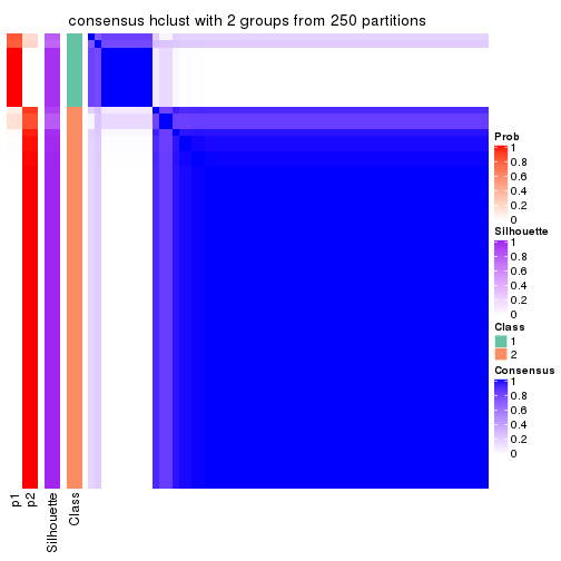
consensus_heatmap(res, k = 3)
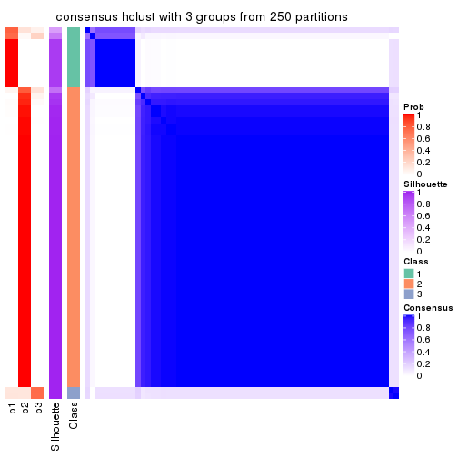
consensus_heatmap(res, k = 4)
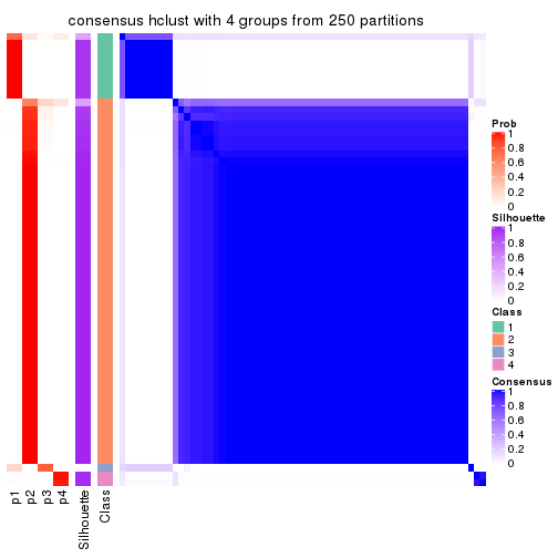
consensus_heatmap(res, k = 5)
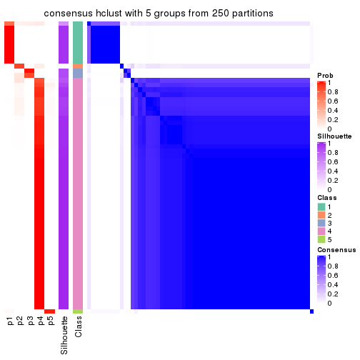
consensus_heatmap(res, k = 6)
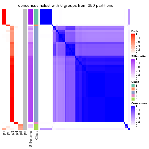
Heatmaps for the membership of samples in all partitions to see how consistent they are:
membership_heatmap(res, k = 2)
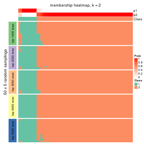
membership_heatmap(res, k = 3)
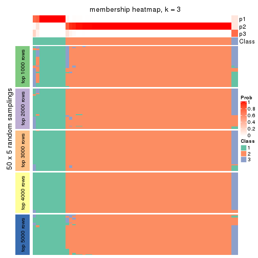
membership_heatmap(res, k = 4)
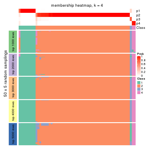
membership_heatmap(res, k = 5)
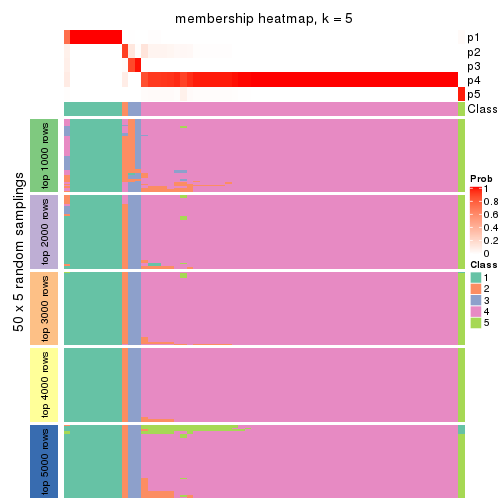
membership_heatmap(res, k = 6)
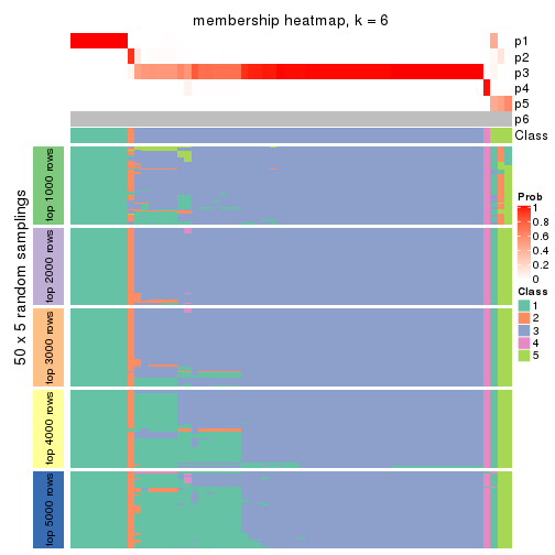
As soon as we have had the classes for columns, we can look for signatures which are significantly different between classes which can be candidate marks for certain classes. Following are the heatmaps for signatures.
Signature heatmaps where rows are scaled:
get_signatures(res, k = 2)
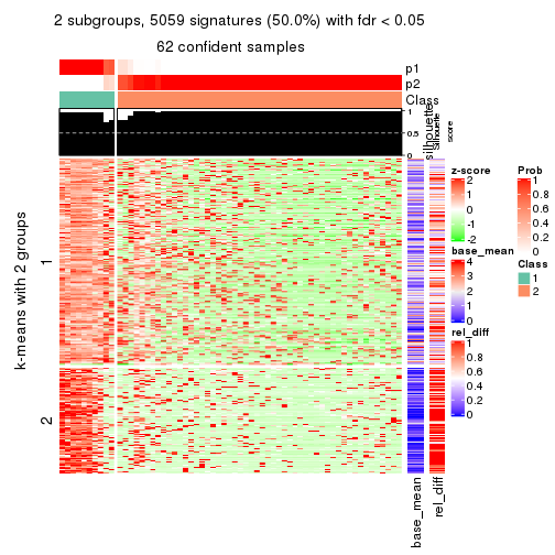
get_signatures(res, k = 3)
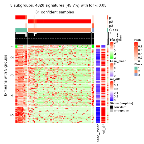
get_signatures(res, k = 4)
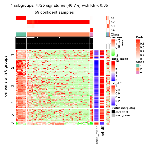
get_signatures(res, k = 5)
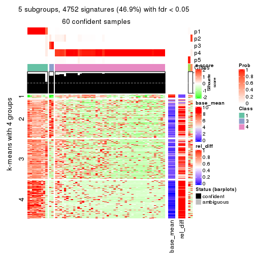
get_signatures(res, k = 6)
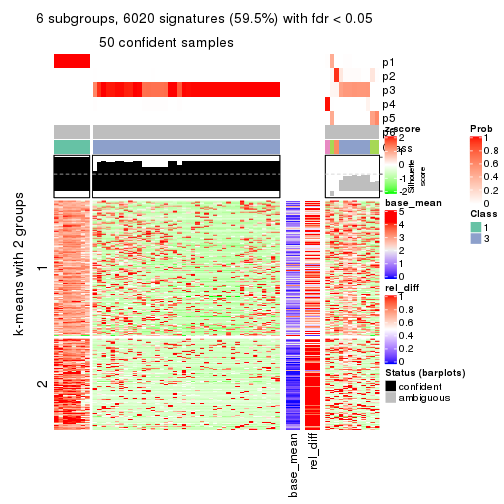
Signature heatmaps where rows are not scaled:
get_signatures(res, k = 2, scale_rows = FALSE)
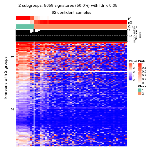
get_signatures(res, k = 3, scale_rows = FALSE)
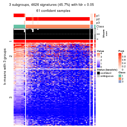
get_signatures(res, k = 4, scale_rows = FALSE)
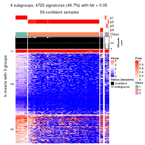
get_signatures(res, k = 5, scale_rows = FALSE)
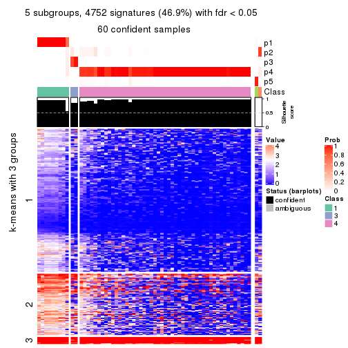
get_signatures(res, k = 6, scale_rows = FALSE)
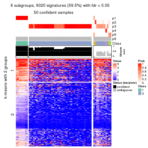
Compare the overlap of signatures from different k:
compare_signatures(res)
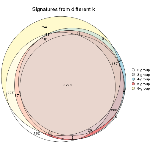
get_signature() returns a data frame invisibly. TO get the list of signatures, the function
call should be assigned to a variable explicitly. In following code, if plot argument is set
to FALSE, no heatmap is plotted while only the differential analysis is performed.
# code only for demonstration
tb = get_signature(res, k = ..., plot = FALSE)
An example of the output of tb is:
#>   which_row         fdr    mean_1    mean_2 scaled_mean_1 scaled_mean_2 km
#> 1        38 0.042760348  8.373488  9.131774    -0.5533452     0.5164555  1
#> 2        40 0.018707592  7.106213  8.469186    -0.6173731     0.5762149  1
#> 3        55 0.019134737 10.221463 11.207825    -0.6159697     0.5749050  1
#> 4        59 0.006059896  5.921854  7.869574    -0.6899429     0.6439467  1
#> 5        60 0.018055526  8.928898 10.211722    -0.6204761     0.5791110  1
#> 6        98 0.009384629 15.714769 14.887706     0.6635654    -0.6193277  2
...
The columns in tb are:
which_row: row indices corresponding to the input matrix.fdr: FDR for the differential test. mean_x: The mean value in group x.scaled_mean_x: The mean value in group x after rows are scaled.km: Row groups if k-means clustering is applied to rows.UMAP plot which shows how samples are separated.
dimension_reduction(res, k = 2, method = "UMAP")
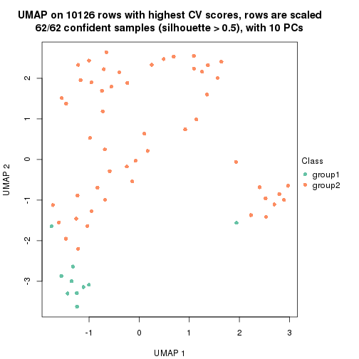
dimension_reduction(res, k = 3, method = "UMAP")
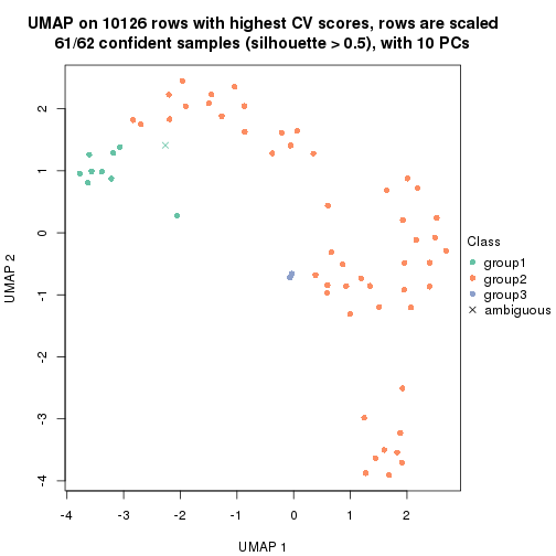
dimension_reduction(res, k = 4, method = "UMAP")
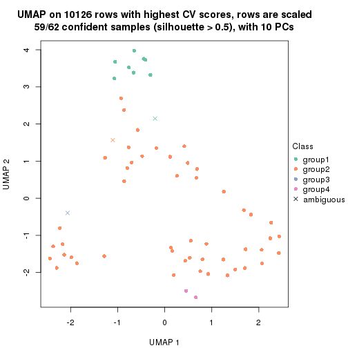
dimension_reduction(res, k = 5, method = "UMAP")

dimension_reduction(res, k = 6, method = "UMAP")
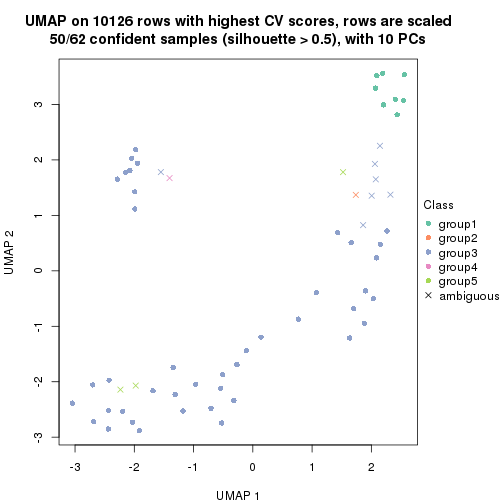
Following heatmap shows how subgroups are split when increasing k:
collect_classes(res)
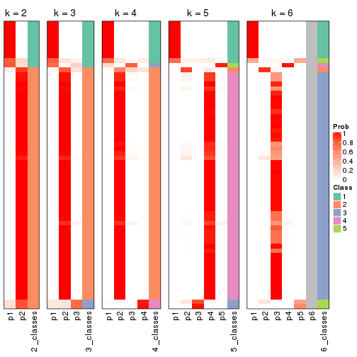
If matrix rows can be associated to genes, consider to use functional_enrichment(res,
...) to perform function enrichment for the signature genes. See this vignette for more detailed explanations.
The object with results only for a single top-value method and a single partition method can be extracted as:
res = res_list["CV", "kmeans"]
# you can also extract it by
# res = res_list["CV:kmeans"]
A summary of res and all the functions that can be applied to it:
res
#> A 'ConsensusPartition' object with k = 2, 3, 4, 5, 6.
#>   On a matrix with 10126 rows and 62 columns.
#>   Top rows (1000, 2000, 3000, 4000, 5000) are extracted by 'CV' method.
#>   Subgroups are detected by 'kmeans' method.
#>   Performed in total 1250 partitions by row resampling.
#>   Best k for subgroups seems to be 3.
#>
#> Following methods can be applied to this 'ConsensusPartition' object:
#>  [1] "cola_report"             "collect_classes"         "collect_plots"
#>  [4] "collect_stats"           "colnames"                "compare_signatures"
#>  [7] "consensus_heatmap"       "dimension_reduction"     "functional_enrichment"
#> [10] "get_anno_col"            "get_anno"                "get_classes"
#> [13] "get_consensus"           "get_matrix"              "get_membership"
#> [16] "get_param"               "get_signatures"          "get_stats"
#> [19] "is_best_k"               "is_stable_k"             "membership_heatmap"
#> [22] "ncol"                    "nrow"                    "plot_ecdf"
#> [25] "rownames"                "select_partition_number" "show"
#> [28] "suggest_best_k"          "test_to_known_factors"
collect_plots() function collects all the plots made from res for all k (number of partitions)
into one single page to provide an easy and fast comparison between different k.
collect_plots(res)
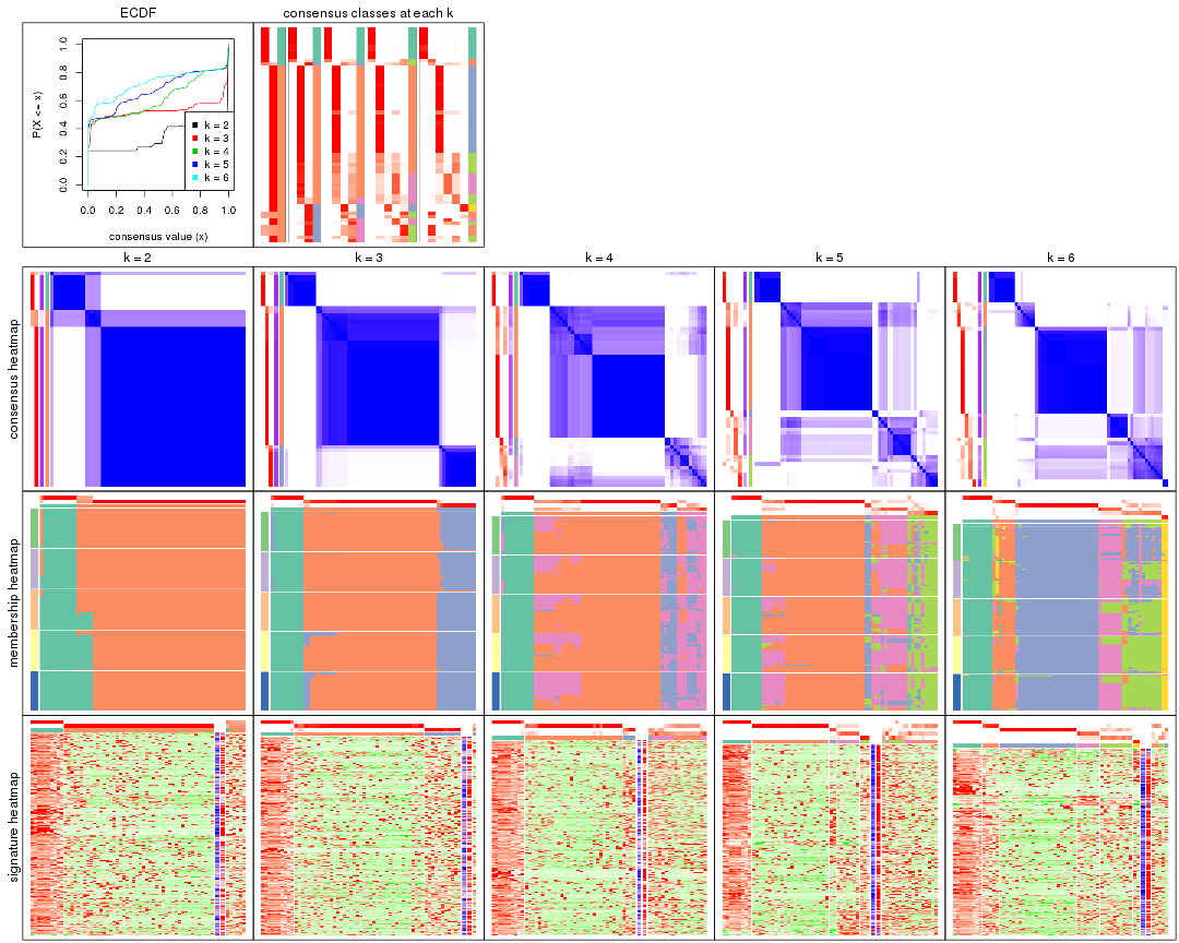
The plots are:
k and the heatmap of
predicted classes for each k.k.k.k.All the plots in panels can be made by individual functions and they are plotted later in this section.
select_partition_number() produces several plots showing different
statistics for choosing “optimized” k. There are following statistics:
k;k, the area increased is defined as \(A_k - A_{k-1}\).The detailed explanations of these statistics can be found in the cola vignette.
Generally speaking, lower PAC score, higher mean silhouette score or higher
concordance corresponds to better partition. Rand index and Jaccard index
measure how similar the current partition is compared to partition with k-1.
If they are too similar, we won't accept k is better than k-1.
select_partition_number(res)
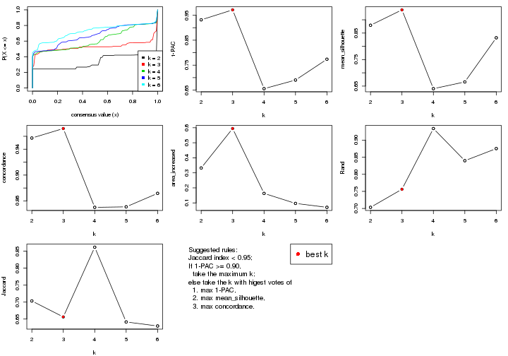
The numeric values for all these statistics can be obtained by get_stats().
get_stats(res)
#>   k 1-PAC mean_silhouette concordance area_increased  Rand Jaccard
#> 2 2 0.932           0.879       0.957         0.3323 0.703   0.703
#> 3 3 0.972           0.938       0.972         0.5946 0.756   0.656
#> 4 4 0.656           0.640       0.850         0.1632 0.934   0.862
#> 5 5 0.690           0.666       0.851         0.0967 0.840   0.641
#> 6 6 0.774           0.832       0.872         0.0707 0.875   0.630
suggest_best_k() suggests the best \(k\) based on these statistics. The rules are as follows:
suggest_best_k(res)
#> [1] 3
#> attr(,"optional")
#> [1] 2
There is also optional best \(k\) = 2 that is worth to check.
Following shows the table of the partitions (You need to click the show/hide
code output link to see it). The membership matrix (columns with name p*)
is inferred by
clue::cl_consensus()
function with the SE method. Basically the value in the membership matrix
represents the probability to belong to a certain group. The finall class
label for an item is determined with the group with highest probability it
belongs to.
In get_classes() function, the entropy is calculated from the membership
matrix and the silhouette score is calculated from the consensus matrix.
cbind(get_classes(res, k = 2), get_membership(res, k = 2))
#>            class entropy silhouette    p1    p2
#> SRR764776      1   0.000      0.961 1.000 0.000
#> SRR764777      1   0.000      0.961 1.000 0.000
#> SRR764778      1   0.000      0.961 1.000 0.000
#> SRR764779      1   0.000      0.961 1.000 0.000
#> SRR764780      1   0.000      0.961 1.000 0.000
#> SRR764781      1   0.000      0.961 1.000 0.000
#> SRR764782      2   0.000      0.950 0.000 1.000
#> SRR764783      2   0.997      0.134 0.468 0.532
#> SRR764784      2   0.000      0.950 0.000 1.000
#> SRR764785      2   0.000      0.950 0.000 1.000
#> SRR764786      2   0.000      0.950 0.000 1.000
#> SRR764787      2   0.000      0.950 0.000 1.000
#> SRR764788      2   0.000      0.950 0.000 1.000
#> SRR764789      2   0.000      0.950 0.000 1.000
#> SRR764790      2   0.000      0.950 0.000 1.000
#> SRR764791      2   0.000      0.950 0.000 1.000
#> SRR764792      2   0.000      0.950 0.000 1.000
#> SRR764793      2   0.000      0.950 0.000 1.000
#> SRR764794      2   0.000      0.950 0.000 1.000
#> SRR764795      2   0.000      0.950 0.000 1.000
#> SRR764796      2   0.000      0.950 0.000 1.000
#> SRR764797      2   0.990      0.220 0.440 0.560
#> SRR764798      2   0.000      0.950 0.000 1.000
#> SRR764799      1   0.000      0.961 1.000 0.000
#> SRR764800      1   0.000      0.961 1.000 0.000
#> SRR764801      2   0.000      0.950 0.000 1.000
#> SRR764802      2   0.995      0.160 0.460 0.540
#> SRR764803      2   0.995      0.160 0.460 0.540
#> SRR764804      2   0.000      0.950 0.000 1.000
#> SRR764805      2   0.000      0.950 0.000 1.000
#> SRR764806      2   0.000      0.950 0.000 1.000
#> SRR764807      2   0.000      0.950 0.000 1.000
#> SRR764808      2   0.000      0.950 0.000 1.000
#> SRR764809      2   0.000      0.950 0.000 1.000
#> SRR764810      2   0.000      0.950 0.000 1.000
#> SRR764811      2   0.000      0.950 0.000 1.000
#> SRR764812      2   0.000      0.950 0.000 1.000
#> SRR764813      2   0.000      0.950 0.000 1.000
#> SRR764814      2   0.997      0.134 0.468 0.532
#> SRR764815      2   0.000      0.950 0.000 1.000
#> SRR764816      1   0.000      0.961 1.000 0.000
#> SRR764817      1   0.000      0.961 1.000 0.000
#> SRR1066622     2   0.000      0.950 0.000 1.000
#> SRR1066623     2   0.000      0.950 0.000 1.000
#> SRR1066624     1   0.936      0.396 0.648 0.352
#> SRR1066625     2   0.000      0.950 0.000 1.000
#> SRR1066626     2   0.000      0.950 0.000 1.000
#> SRR1066627     2   0.000      0.950 0.000 1.000
#> SRR1066628     2   0.000      0.950 0.000 1.000
#> SRR1066629     2   0.000      0.950 0.000 1.000
#> SRR1066630     2   0.000      0.950 0.000 1.000
#> SRR1066631     2   0.000      0.950 0.000 1.000
#> SRR1066632     2   0.000      0.950 0.000 1.000
#> SRR1066633     2   0.000      0.950 0.000 1.000
#> SRR1066634     2   0.000      0.950 0.000 1.000
#> SRR1066635     2   0.000      0.950 0.000 1.000
#> SRR1066636     2   0.000      0.950 0.000 1.000
#> SRR1066637     2   0.000      0.950 0.000 1.000
#> SRR1066638     2   0.000      0.950 0.000 1.000
#> SRR1066639     2   0.000      0.950 0.000 1.000
#> SRR1066640     2   0.000      0.950 0.000 1.000
#> SRR1066641     2   0.000      0.950 0.000 1.000
cbind(get_classes(res, k = 3), get_membership(res, k = 3))
#>            class entropy silhouette    p1    p2    p3
#> SRR764776      1  0.0000      0.972 1.000 0.000 0.000
#> SRR764777      1  0.0000      0.972 1.000 0.000 0.000
#> SRR764778      1  0.0000      0.972 1.000 0.000 0.000
#> SRR764779      1  0.0000      0.972 1.000 0.000 0.000
#> SRR764780      1  0.0000      0.972 1.000 0.000 0.000
#> SRR764781      1  0.4974      0.703 0.764 0.000 0.236
#> SRR764782      2  0.5431      0.603 0.000 0.716 0.284
#> SRR764783      3  0.0592      0.931 0.000 0.012 0.988
#> SRR764784      2  0.5138      0.664 0.000 0.748 0.252
#> SRR764785      2  0.0000      0.977 0.000 1.000 0.000
#> SRR764786      2  0.0000      0.977 0.000 1.000 0.000
#> SRR764787      2  0.0237      0.974 0.000 0.996 0.004
#> SRR764788      3  0.5988      0.416 0.000 0.368 0.632
#> SRR764789      2  0.0000      0.977 0.000 1.000 0.000
#> SRR764790      2  0.0000      0.977 0.000 1.000 0.000
#> SRR764791      2  0.0000      0.977 0.000 1.000 0.000
#> SRR764792      2  0.1411      0.955 0.000 0.964 0.036
#> SRR764793      2  0.2066      0.933 0.000 0.940 0.060
#> SRR764794      2  0.1031      0.962 0.000 0.976 0.024
#> SRR764795      3  0.0592      0.931 0.000 0.012 0.988
#> SRR764796      3  0.3192      0.811 0.000 0.112 0.888
#> SRR764797      3  0.0592      0.931 0.000 0.012 0.988
#> SRR764798      3  0.0592      0.931 0.000 0.012 0.988
#> SRR764799      1  0.0592      0.967 0.988 0.000 0.012
#> SRR764800      1  0.0592      0.967 0.988 0.000 0.012
#> SRR764801      3  0.0592      0.931 0.000 0.012 0.988
#> SRR764802      3  0.0592      0.931 0.000 0.012 0.988
#> SRR764803      3  0.0592      0.931 0.000 0.012 0.988
#> SRR764804      2  0.0000      0.977 0.000 1.000 0.000
#> SRR764805      2  0.0000      0.977 0.000 1.000 0.000
#> SRR764806      2  0.0000      0.977 0.000 1.000 0.000
#> SRR764807      2  0.0000      0.977 0.000 1.000 0.000
#> SRR764808      2  0.0000      0.977 0.000 1.000 0.000
#> SRR764809      2  0.0000      0.977 0.000 1.000 0.000
#> SRR764810      2  0.0000      0.977 0.000 1.000 0.000
#> SRR764811      2  0.0000      0.977 0.000 1.000 0.000
#> SRR764812      2  0.0000      0.977 0.000 1.000 0.000
#> SRR764813      2  0.0000      0.977 0.000 1.000 0.000
#> SRR764814      3  0.0592      0.931 0.000 0.012 0.988
#> SRR764815      2  0.1289      0.957 0.000 0.968 0.032
#> SRR764816      1  0.0000      0.972 1.000 0.000 0.000
#> SRR764817      1  0.0000      0.972 1.000 0.000 0.000
#> SRR1066622     2  0.1529      0.952 0.000 0.960 0.040
#> SRR1066623     2  0.1529      0.952 0.000 0.960 0.040
#> SRR1066624     3  0.0661      0.919 0.008 0.004 0.988
#> SRR1066625     3  0.0747      0.928 0.000 0.016 0.984
#> SRR1066626     2  0.0000      0.977 0.000 1.000 0.000
#> SRR1066627     2  0.1964      0.939 0.000 0.944 0.056
#> SRR1066628     2  0.0000      0.977 0.000 1.000 0.000
#> SRR1066629     2  0.1529      0.952 0.000 0.960 0.040
#> SRR1066630     2  0.0000      0.977 0.000 1.000 0.000
#> SRR1066631     2  0.0237      0.974 0.000 0.996 0.004
#> SRR1066632     2  0.0000      0.977 0.000 1.000 0.000
#> SRR1066633     2  0.0000      0.977 0.000 1.000 0.000
#> SRR1066634     2  0.0000      0.977 0.000 1.000 0.000
#> SRR1066635     2  0.0000      0.977 0.000 1.000 0.000
#> SRR1066636     2  0.0000      0.977 0.000 1.000 0.000
#> SRR1066637     2  0.0000      0.977 0.000 1.000 0.000
#> SRR1066638     2  0.0000      0.977 0.000 1.000 0.000
#> SRR1066639     2  0.0000      0.977 0.000 1.000 0.000
#> SRR1066640     2  0.0000      0.977 0.000 1.000 0.000
#> SRR1066641     2  0.0000      0.977 0.000 1.000 0.000
cbind(get_classes(res, k = 4), get_membership(res, k = 4))
#>            class entropy silhouette    p1    p2    p3    p4
#> SRR764776      1  0.0000     0.9636 1.000 0.000 0.000 0.000
#> SRR764777      1  0.0000     0.9636 1.000 0.000 0.000 0.000
#> SRR764778      1  0.0000     0.9636 1.000 0.000 0.000 0.000
#> SRR764779      1  0.0000     0.9636 1.000 0.000 0.000 0.000
#> SRR764780      1  0.0000     0.9636 1.000 0.000 0.000 0.000
#> SRR764781      1  0.5798     0.5773 0.704 0.000 0.112 0.184
#> SRR764782      4  0.5581    -0.0502 0.000 0.448 0.020 0.532
#> SRR764783      4  0.4916    -0.3949 0.000 0.000 0.424 0.576
#> SRR764784      4  0.5376     0.0891 0.000 0.396 0.016 0.588
#> SRR764785      2  0.0000     0.8392 0.000 1.000 0.000 0.000
#> SRR764786      2  0.0000     0.8392 0.000 1.000 0.000 0.000
#> SRR764787      2  0.4018     0.6938 0.000 0.772 0.004 0.224
#> SRR764788      4  0.6058     0.3714 0.000 0.296 0.072 0.632
#> SRR764789      2  0.3975     0.6793 0.000 0.760 0.000 0.240
#> SRR764790      2  0.0000     0.8392 0.000 1.000 0.000 0.000
#> SRR764791      2  0.3444     0.7274 0.000 0.816 0.000 0.184
#> SRR764792      2  0.5220     0.3864 0.000 0.568 0.008 0.424
#> SRR764793      2  0.5339     0.4530 0.000 0.600 0.016 0.384
#> SRR764794      2  0.4456     0.6361 0.000 0.716 0.004 0.280
#> SRR764795      4  0.2011     0.2508 0.000 0.000 0.080 0.920
#> SRR764796      4  0.1584     0.3117 0.000 0.036 0.012 0.952
#> SRR764797      3  0.4967     0.4565 0.000 0.000 0.548 0.452
#> SRR764798      3  0.0592     0.7362 0.000 0.000 0.984 0.016
#> SRR764799      1  0.0336     0.9599 0.992 0.000 0.008 0.000
#> SRR764800      1  0.0336     0.9599 0.992 0.000 0.008 0.000
#> SRR764801      3  0.0592     0.7362 0.000 0.000 0.984 0.016
#> SRR764802      4  0.4941    -0.4102 0.000 0.000 0.436 0.564
#> SRR764803      4  0.4972    -0.4490 0.000 0.000 0.456 0.544
#> SRR764804      2  0.0000     0.8392 0.000 1.000 0.000 0.000
#> SRR764805      2  0.0000     0.8392 0.000 1.000 0.000 0.000
#> SRR764806      2  0.0000     0.8392 0.000 1.000 0.000 0.000
#> SRR764807      2  0.0000     0.8392 0.000 1.000 0.000 0.000
#> SRR764808      2  0.0000     0.8392 0.000 1.000 0.000 0.000
#> SRR764809      2  0.0000     0.8392 0.000 1.000 0.000 0.000
#> SRR764810      2  0.0000     0.8392 0.000 1.000 0.000 0.000
#> SRR764811      2  0.0000     0.8392 0.000 1.000 0.000 0.000
#> SRR764812      2  0.0000     0.8392 0.000 1.000 0.000 0.000
#> SRR764813      2  0.0000     0.8392 0.000 1.000 0.000 0.000
#> SRR764814      3  0.3444     0.7389 0.000 0.000 0.816 0.184
#> SRR764815      2  0.4509     0.6264 0.000 0.708 0.004 0.288
#> SRR764816      1  0.0000     0.9636 1.000 0.000 0.000 0.000
#> SRR764817      1  0.0000     0.9636 1.000 0.000 0.000 0.000
#> SRR1066622     2  0.5151     0.3563 0.000 0.532 0.004 0.464
#> SRR1066623     2  0.5143     0.3740 0.000 0.540 0.004 0.456
#> SRR1066624     3  0.4713     0.6463 0.000 0.000 0.640 0.360
#> SRR1066625     4  0.4252     0.0400 0.000 0.004 0.252 0.744
#> SRR1066626     2  0.3486     0.7240 0.000 0.812 0.000 0.188
#> SRR1066627     2  0.5163     0.3156 0.000 0.516 0.004 0.480
#> SRR1066628     2  0.5070     0.4513 0.000 0.580 0.004 0.416
#> SRR1066629     2  0.5137     0.3828 0.000 0.544 0.004 0.452
#> SRR1066630     2  0.0000     0.8392 0.000 1.000 0.000 0.000
#> SRR1066631     2  0.4925     0.4372 0.000 0.572 0.000 0.428
#> SRR1066632     2  0.0000     0.8392 0.000 1.000 0.000 0.000
#> SRR1066633     2  0.0000     0.8392 0.000 1.000 0.000 0.000
#> SRR1066634     2  0.0000     0.8392 0.000 1.000 0.000 0.000
#> SRR1066635     2  0.0000     0.8392 0.000 1.000 0.000 0.000
#> SRR1066636     2  0.0000     0.8392 0.000 1.000 0.000 0.000
#> SRR1066637     2  0.0000     0.8392 0.000 1.000 0.000 0.000
#> SRR1066638     2  0.0000     0.8392 0.000 1.000 0.000 0.000
#> SRR1066639     2  0.0000     0.8392 0.000 1.000 0.000 0.000
#> SRR1066640     2  0.0000     0.8392 0.000 1.000 0.000 0.000
#> SRR1066641     2  0.0000     0.8392 0.000 1.000 0.000 0.000
cbind(get_classes(res, k = 5), get_membership(res, k = 5))
#>            class entropy silhouette    p1    p2    p3    p4    p5
#> SRR764776      1  0.0000     0.9917 1.000 0.000 0.000 0.000 0.000
#> SRR764777      1  0.0000     0.9917 1.000 0.000 0.000 0.000 0.000
#> SRR764778      1  0.0000     0.9917 1.000 0.000 0.000 0.000 0.000
#> SRR764779      1  0.0000     0.9917 1.000 0.000 0.000 0.000 0.000
#> SRR764780      1  0.0000     0.9917 1.000 0.000 0.000 0.000 0.000
#> SRR764781      5  0.4420     0.0595 0.448 0.000 0.000 0.004 0.548
#> SRR764782      4  0.7733     0.4190 0.000 0.364 0.072 0.368 0.196
#> SRR764783      5  0.0880     0.5211 0.000 0.000 0.000 0.032 0.968
#> SRR764784      4  0.7195     0.5671 0.000 0.276 0.060 0.508 0.156
#> SRR764785      2  0.0000     0.8673 0.000 1.000 0.000 0.000 0.000
#> SRR764786      2  0.0000     0.8673 0.000 1.000 0.000 0.000 0.000
#> SRR764787      2  0.5517     0.2210 0.000 0.608 0.068 0.316 0.008
#> SRR764788      5  0.7825    -0.2633 0.000 0.228 0.080 0.276 0.416
#> SRR764789      2  0.5478     0.1549 0.000 0.592 0.068 0.336 0.004
#> SRR764790      2  0.0000     0.8673 0.000 1.000 0.000 0.000 0.000
#> SRR764791      2  0.5090     0.3721 0.000 0.668 0.064 0.264 0.004
#> SRR764792      4  0.7640     0.4362 0.000 0.360 0.080 0.400 0.160
#> SRR764793      2  0.6838    -0.2375 0.000 0.472 0.068 0.384 0.076
#> SRR764794      2  0.6174    -0.0379 0.000 0.536 0.080 0.360 0.024
#> SRR764795      5  0.5320     0.1988 0.000 0.000 0.060 0.368 0.572
#> SRR764796      4  0.4192     0.4461 0.000 0.008 0.048 0.780 0.164
#> SRR764797      5  0.2172     0.4709 0.000 0.000 0.076 0.016 0.908
#> SRR764798      3  0.2280     0.9930 0.000 0.000 0.880 0.000 0.120
#> SRR764799      1  0.1106     0.9704 0.964 0.000 0.012 0.024 0.000
#> SRR764800      1  0.1106     0.9704 0.964 0.000 0.012 0.024 0.000
#> SRR764801      3  0.2230     0.9931 0.000 0.000 0.884 0.000 0.116
#> SRR764802      5  0.0880     0.5211 0.000 0.000 0.000 0.032 0.968
#> SRR764803      5  0.0404     0.5168 0.000 0.000 0.000 0.012 0.988
#> SRR764804      2  0.0000     0.8673 0.000 1.000 0.000 0.000 0.000
#> SRR764805      2  0.0000     0.8673 0.000 1.000 0.000 0.000 0.000
#> SRR764806      2  0.0451     0.8605 0.000 0.988 0.008 0.004 0.000
#> SRR764807      2  0.0000     0.8673 0.000 1.000 0.000 0.000 0.000
#> SRR764808      2  0.0000     0.8673 0.000 1.000 0.000 0.000 0.000
#> SRR764809      2  0.0000     0.8673 0.000 1.000 0.000 0.000 0.000
#> SRR764810      2  0.0000     0.8673 0.000 1.000 0.000 0.000 0.000
#> SRR764811      2  0.0000     0.8673 0.000 1.000 0.000 0.000 0.000
#> SRR764812      2  0.0000     0.8673 0.000 1.000 0.000 0.000 0.000
#> SRR764813      2  0.0000     0.8673 0.000 1.000 0.000 0.000 0.000
#> SRR764814      5  0.4630    -0.0958 0.000 0.000 0.396 0.016 0.588
#> SRR764815      2  0.6210     0.0108 0.000 0.548 0.068 0.348 0.036
#> SRR764816      1  0.0000     0.9917 1.000 0.000 0.000 0.000 0.000
#> SRR764817      1  0.0000     0.9917 1.000 0.000 0.000 0.000 0.000
#> SRR1066622     4  0.3039     0.7513 0.000 0.192 0.000 0.808 0.000
#> SRR1066623     4  0.3109     0.7554 0.000 0.200 0.000 0.800 0.000
#> SRR1066624     5  0.6275     0.0511 0.000 0.000 0.176 0.308 0.516
#> SRR1066625     4  0.3401     0.3837 0.000 0.008 0.072 0.852 0.068
#> SRR1066626     2  0.3857     0.3938 0.000 0.688 0.000 0.312 0.000
#> SRR1066627     4  0.3086     0.7403 0.000 0.180 0.000 0.816 0.004
#> SRR1066628     4  0.3274     0.7492 0.000 0.220 0.000 0.780 0.000
#> SRR1066629     4  0.3109     0.7554 0.000 0.200 0.000 0.800 0.000
#> SRR1066630     2  0.0000     0.8673 0.000 1.000 0.000 0.000 0.000
#> SRR1066631     4  0.3210     0.7531 0.000 0.212 0.000 0.788 0.000
#> SRR1066632     2  0.0000     0.8673 0.000 1.000 0.000 0.000 0.000
#> SRR1066633     2  0.0404     0.8604 0.000 0.988 0.012 0.000 0.000
#> SRR1066634     2  0.0162     0.8645 0.000 0.996 0.000 0.004 0.000
#> SRR1066635     2  0.0162     0.8657 0.000 0.996 0.004 0.000 0.000
#> SRR1066636     2  0.0162     0.8657 0.000 0.996 0.004 0.000 0.000
#> SRR1066637     2  0.0000     0.8673 0.000 1.000 0.000 0.000 0.000
#> SRR1066638     2  0.0162     0.8657 0.000 0.996 0.004 0.000 0.000
#> SRR1066639     2  0.0162     0.8657 0.000 0.996 0.004 0.000 0.000
#> SRR1066640     2  0.0162     0.8657 0.000 0.996 0.004 0.000 0.000
#> SRR1066641     2  0.0000     0.8673 0.000 1.000 0.000 0.000 0.000
cbind(get_classes(res, k = 6), get_membership(res, k = 6))
#>            class entropy silhouette    p1    p2    p3    p4    p5    p6
#> SRR764776      1  0.0000      0.990 1.000 0.000 0.000 0.000 0.000 0.000
#> SRR764777      1  0.0000      0.990 1.000 0.000 0.000 0.000 0.000 0.000
#> SRR764778      1  0.0000      0.990 1.000 0.000 0.000 0.000 0.000 0.000
#> SRR764779      1  0.0000      0.990 1.000 0.000 0.000 0.000 0.000 0.000
#> SRR764780      1  0.0000      0.990 1.000 0.000 0.000 0.000 0.000 0.000
#> SRR764781      2  0.2730      0.648 0.192 0.808 0.000 0.000 0.000 0.000
#> SRR764782      5  0.4130      0.702 0.000 0.024 0.260 0.012 0.704 0.000
#> SRR764783      2  0.1219      0.789 0.000 0.948 0.000 0.004 0.048 0.000
#> SRR764784      5  0.5010      0.605 0.000 0.020 0.192 0.108 0.680 0.000
#> SRR764785      3  0.0000      0.977 0.000 0.000 1.000 0.000 0.000 0.000
#> SRR764786      3  0.0000      0.977 0.000 0.000 1.000 0.000 0.000 0.000
#> SRR764787      5  0.4051      0.618 0.000 0.000 0.432 0.008 0.560 0.000
#> SRR764788      5  0.5585      0.573 0.000 0.204 0.176 0.016 0.604 0.000
#> SRR764789      5  0.4531      0.643 0.000 0.000 0.408 0.036 0.556 0.000
#> SRR764790      3  0.0000      0.977 0.000 0.000 1.000 0.000 0.000 0.000
#> SRR764791      5  0.3993      0.534 0.000 0.000 0.476 0.004 0.520 0.000
#> SRR764792      5  0.4770      0.656 0.000 0.052 0.204 0.032 0.708 0.004
#> SRR764793      5  0.4140      0.706 0.000 0.008 0.280 0.024 0.688 0.000
#> SRR764794      5  0.4165      0.706 0.000 0.000 0.292 0.028 0.676 0.004
#> SRR764795      5  0.4802     -0.108 0.000 0.452 0.000 0.052 0.496 0.000
#> SRR764796      5  0.4355     -0.258 0.000 0.024 0.000 0.420 0.556 0.000
#> SRR764797      2  0.1010      0.777 0.000 0.960 0.000 0.000 0.004 0.036
#> SRR764798      6  0.0914      0.988 0.000 0.016 0.000 0.000 0.016 0.968
#> SRR764799      1  0.1230      0.964 0.956 0.000 0.000 0.008 0.028 0.008
#> SRR764800      1  0.1230      0.964 0.956 0.000 0.000 0.008 0.028 0.008
#> SRR764801      6  0.0458      0.988 0.000 0.016 0.000 0.000 0.000 0.984
#> SRR764802      2  0.1219      0.789 0.000 0.948 0.000 0.004 0.048 0.000
#> SRR764803      2  0.0790      0.790 0.000 0.968 0.000 0.000 0.032 0.000
#> SRR764804      3  0.0000      0.977 0.000 0.000 1.000 0.000 0.000 0.000
#> SRR764805      3  0.0000      0.977 0.000 0.000 1.000 0.000 0.000 0.000
#> SRR764806      3  0.0363      0.969 0.000 0.000 0.988 0.000 0.012 0.000
#> SRR764807      3  0.0000      0.977 0.000 0.000 1.000 0.000 0.000 0.000
#> SRR764808      3  0.0000      0.977 0.000 0.000 1.000 0.000 0.000 0.000
#> SRR764809      3  0.0000      0.977 0.000 0.000 1.000 0.000 0.000 0.000
#> SRR764810      3  0.0000      0.977 0.000 0.000 1.000 0.000 0.000 0.000
#> SRR764811      3  0.0000      0.977 0.000 0.000 1.000 0.000 0.000 0.000
#> SRR764812      3  0.0000      0.977 0.000 0.000 1.000 0.000 0.000 0.000
#> SRR764813      3  0.0000      0.977 0.000 0.000 1.000 0.000 0.000 0.000
#> SRR764814      2  0.3844      0.489 0.000 0.676 0.000 0.004 0.008 0.312
#> SRR764815      5  0.4193      0.691 0.000 0.000 0.352 0.024 0.624 0.000
#> SRR764816      1  0.0000      0.990 1.000 0.000 0.000 0.000 0.000 0.000
#> SRR764817      1  0.0000      0.990 1.000 0.000 0.000 0.000 0.000 0.000
#> SRR1066622     4  0.3683      0.944 0.000 0.000 0.048 0.768 0.184 0.000
#> SRR1066623     4  0.3715      0.945 0.000 0.000 0.048 0.764 0.188 0.000
#> SRR1066624     2  0.6136      0.387 0.000 0.512 0.000 0.252 0.216 0.020
#> SRR1066625     4  0.1909      0.684 0.000 0.024 0.000 0.920 0.052 0.004
#> SRR1066626     3  0.4762      0.291 0.000 0.000 0.676 0.176 0.148 0.000
#> SRR1066627     4  0.3746      0.944 0.000 0.000 0.048 0.760 0.192 0.000
#> SRR1066628     4  0.3837      0.938 0.000 0.000 0.052 0.752 0.196 0.000
#> SRR1066629     4  0.3683      0.944 0.000 0.000 0.048 0.768 0.184 0.000
#> SRR1066630     3  0.0000      0.977 0.000 0.000 1.000 0.000 0.000 0.000
#> SRR1066631     4  0.3776      0.942 0.000 0.000 0.048 0.756 0.196 0.000
#> SRR1066632     3  0.0146      0.976 0.000 0.000 0.996 0.000 0.004 0.000
#> SRR1066633     3  0.0713      0.949 0.000 0.000 0.972 0.000 0.028 0.000
#> SRR1066634     3  0.0363      0.969 0.000 0.000 0.988 0.000 0.012 0.000
#> SRR1066635     3  0.0146      0.976 0.000 0.000 0.996 0.000 0.004 0.000
#> SRR1066636     3  0.0146      0.976 0.000 0.000 0.996 0.000 0.004 0.000
#> SRR1066637     3  0.0146      0.976 0.000 0.000 0.996 0.000 0.004 0.000
#> SRR1066638     3  0.0146      0.976 0.000 0.000 0.996 0.000 0.004 0.000
#> SRR1066639     3  0.0146      0.976 0.000 0.000 0.996 0.000 0.004 0.000
#> SRR1066640     3  0.0146      0.976 0.000 0.000 0.996 0.000 0.004 0.000
#> SRR1066641     3  0.0000      0.977 0.000 0.000 1.000 0.000 0.000 0.000
Heatmaps for the consensus matrix. It visualizes the probability of two samples to be in a same group.
consensus_heatmap(res, k = 2)
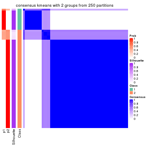
consensus_heatmap(res, k = 3)
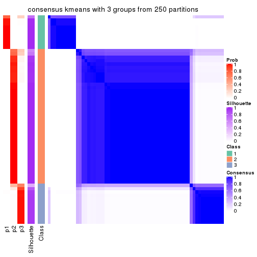
consensus_heatmap(res, k = 4)
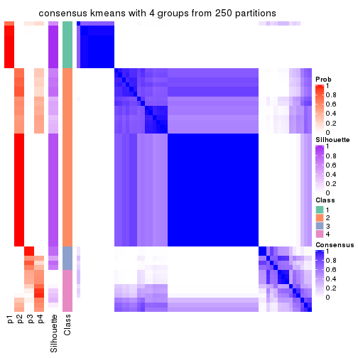
consensus_heatmap(res, k = 5)
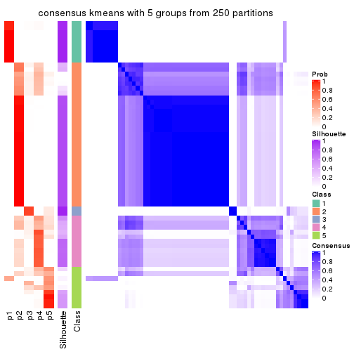
consensus_heatmap(res, k = 6)
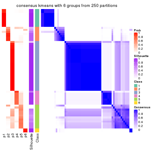
Heatmaps for the membership of samples in all partitions to see how consistent they are:
membership_heatmap(res, k = 2)
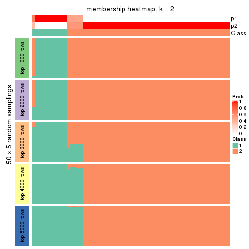
membership_heatmap(res, k = 3)
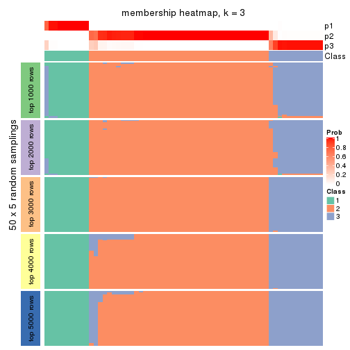
membership_heatmap(res, k = 4)
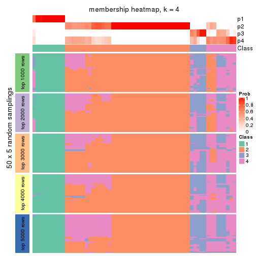
membership_heatmap(res, k = 5)
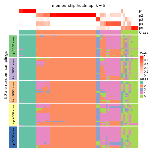
membership_heatmap(res, k = 6)
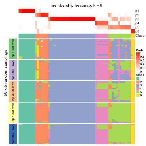
As soon as we have had the classes for columns, we can look for signatures which are significantly different between classes which can be candidate marks for certain classes. Following are the heatmaps for signatures.
Signature heatmaps where rows are scaled:
get_signatures(res, k = 2)

get_signatures(res, k = 3)
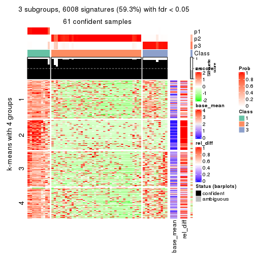
get_signatures(res, k = 4)
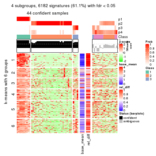
get_signatures(res, k = 5)
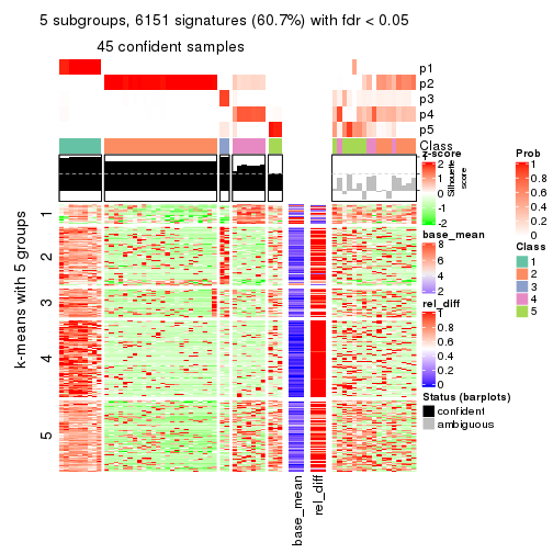
get_signatures(res, k = 6)
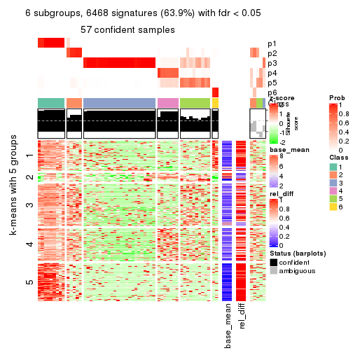
Signature heatmaps where rows are not scaled:
get_signatures(res, k = 2, scale_rows = FALSE)
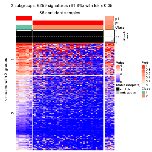
get_signatures(res, k = 3, scale_rows = FALSE)
#> Error in mat[ceiling(1:nr/h_ratio), ceiling(1:nc/w_ratio), drop = FALSE]: subscript out of bounds
get_signatures(res, k = 4, scale_rows = FALSE)
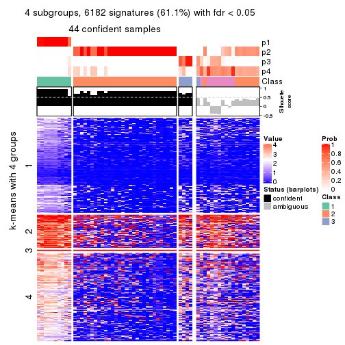
get_signatures(res, k = 5, scale_rows = FALSE)
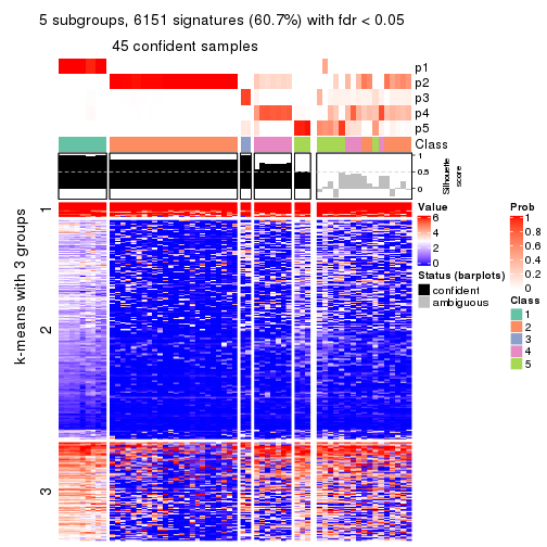
get_signatures(res, k = 6, scale_rows = FALSE)
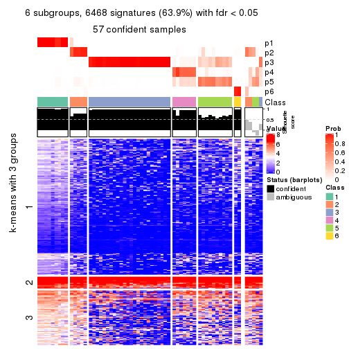
Compare the overlap of signatures from different k:
compare_signatures(res)
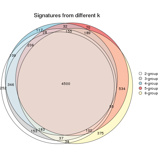
get_signature() returns a data frame invisibly. TO get the list of signatures, the function
call should be assigned to a variable explicitly. In following code, if plot argument is set
to FALSE, no heatmap is plotted while only the differential analysis is performed.
# code only for demonstration
tb = get_signature(res, k = ..., plot = FALSE)
An example of the output of tb is:
#>   which_row         fdr    mean_1    mean_2 scaled_mean_1 scaled_mean_2 km
#> 1        38 0.042760348  8.373488  9.131774    -0.5533452     0.5164555  1
#> 2        40 0.018707592  7.106213  8.469186    -0.6173731     0.5762149  1
#> 3        55 0.019134737 10.221463 11.207825    -0.6159697     0.5749050  1
#> 4        59 0.006059896  5.921854  7.869574    -0.6899429     0.6439467  1
#> 5        60 0.018055526  8.928898 10.211722    -0.6204761     0.5791110  1
#> 6        98 0.009384629 15.714769 14.887706     0.6635654    -0.6193277  2
...
The columns in tb are:
which_row: row indices corresponding to the input matrix.fdr: FDR for the differential test. mean_x: The mean value in group x.scaled_mean_x: The mean value in group x after rows are scaled.km: Row groups if k-means clustering is applied to rows.UMAP plot which shows how samples are separated.
dimension_reduction(res, k = 2, method = "UMAP")

dimension_reduction(res, k = 3, method = "UMAP")
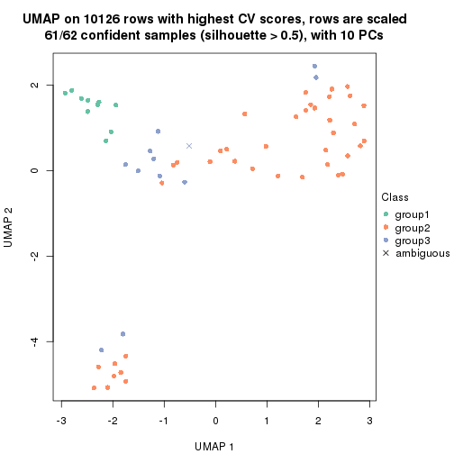
dimension_reduction(res, k = 4, method = "UMAP")
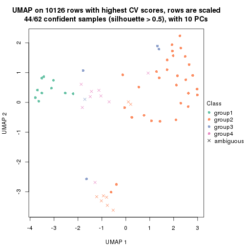
dimension_reduction(res, k = 5, method = "UMAP")
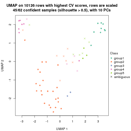
dimension_reduction(res, k = 6, method = "UMAP")
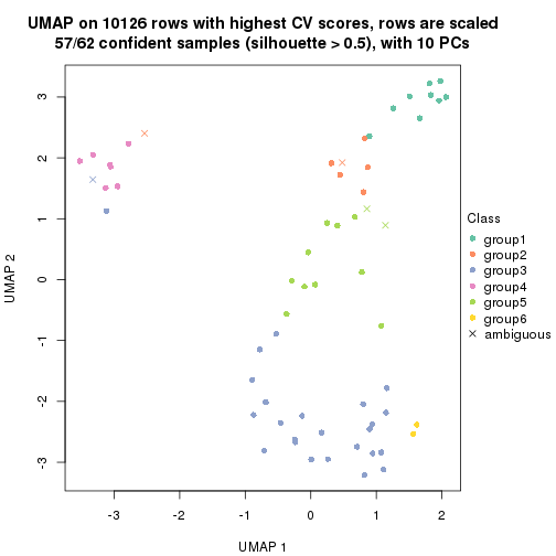
Following heatmap shows how subgroups are split when increasing k:
collect_classes(res)
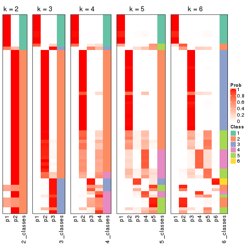
If matrix rows can be associated to genes, consider to use functional_enrichment(res,
...) to perform function enrichment for the signature genes. See this vignette for more detailed explanations.
The object with results only for a single top-value method and a single partition method can be extracted as:
res = res_list["CV", "skmeans"]
# you can also extract it by
# res = res_list["CV:skmeans"]
A summary of res and all the functions that can be applied to it:
res
#> A 'ConsensusPartition' object with k = 2, 3, 4, 5, 6.
#>   On a matrix with 10126 rows and 62 columns.
#>   Top rows (1000, 2000, 3000, 4000, 5000) are extracted by 'CV' method.
#>   Subgroups are detected by 'skmeans' method.
#>   Performed in total 1250 partitions by row resampling.
#>   Best k for subgroups seems to be 2.
#>
#> Following methods can be applied to this 'ConsensusPartition' object:
#>  [1] "cola_report"             "collect_classes"         "collect_plots"
#>  [4] "collect_stats"           "colnames"                "compare_signatures"
#>  [7] "consensus_heatmap"       "dimension_reduction"     "functional_enrichment"
#> [10] "get_anno_col"            "get_anno"                "get_classes"
#> [13] "get_consensus"           "get_matrix"              "get_membership"
#> [16] "get_param"               "get_signatures"          "get_stats"
#> [19] "is_best_k"               "is_stable_k"             "membership_heatmap"
#> [22] "ncol"                    "nrow"                    "plot_ecdf"
#> [25] "rownames"                "select_partition_number" "show"
#> [28] "suggest_best_k"          "test_to_known_factors"
collect_plots() function collects all the plots made from res for all k (number of partitions)
into one single page to provide an easy and fast comparison between different k.
collect_plots(res)

The plots are:
k and the heatmap of
predicted classes for each k.k.k.k.All the plots in panels can be made by individual functions and they are plotted later in this section.
select_partition_number() produces several plots showing different
statistics for choosing “optimized” k. There are following statistics:
k;k, the area increased is defined as \(A_k - A_{k-1}\).The detailed explanations of these statistics can be found in the cola vignette.
Generally speaking, lower PAC score, higher mean silhouette score or higher
concordance corresponds to better partition. Rand index and Jaccard index
measure how similar the current partition is compared to partition with k-1.
If they are too similar, we won't accept k is better than k-1.
select_partition_number(res)
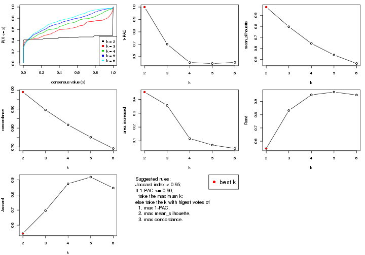
The numeric values for all these statistics can be obtained by get_stats().
get_stats(res)
#>   k 1-PAC mean_silhouette concordance area_increased  Rand Jaccard
#> 2 2 1.000           0.975       0.990         0.4537 0.545   0.545
#> 3 3 0.701           0.797       0.896         0.3566 0.832   0.696
#> 4 4 0.552           0.645       0.817         0.1168 0.950   0.874
#> 5 5 0.544           0.540       0.752         0.0695 0.971   0.919
#> 6 6 0.553           0.463       0.692         0.0445 0.949   0.846
suggest_best_k() suggests the best \(k\) based on these statistics. The rules are as follows:
suggest_best_k(res)
#> [1] 2
Following shows the table of the partitions (You need to click the show/hide
code output link to see it). The membership matrix (columns with name p*)
is inferred by
clue::cl_consensus()
function with the SE method. Basically the value in the membership matrix
represents the probability to belong to a certain group. The finall class
label for an item is determined with the group with highest probability it
belongs to.
In get_classes() function, the entropy is calculated from the membership
matrix and the silhouette score is calculated from the consensus matrix.
cbind(get_classes(res, k = 2), get_membership(res, k = 2))
#>            class entropy silhouette    p1    p2
#> SRR764776      1  0.0000      0.980 1.000 0.000
#> SRR764777      1  0.0000      0.980 1.000 0.000
#> SRR764778      1  0.0000      0.980 1.000 0.000
#> SRR764779      1  0.0000      0.980 1.000 0.000
#> SRR764780      1  0.0000      0.980 1.000 0.000
#> SRR764781      1  0.0000      0.980 1.000 0.000
#> SRR764782      2  0.0000      0.994 0.000 1.000
#> SRR764783      1  0.0000      0.980 1.000 0.000
#> SRR764784      2  0.0000      0.994 0.000 1.000
#> SRR764785      2  0.0000      0.994 0.000 1.000
#> SRR764786      2  0.0000      0.994 0.000 1.000
#> SRR764787      2  0.0000      0.994 0.000 1.000
#> SRR764788      1  0.9661      0.348 0.608 0.392
#> SRR764789      2  0.0000      0.994 0.000 1.000
#> SRR764790      2  0.0000      0.994 0.000 1.000
#> SRR764791      2  0.0000      0.994 0.000 1.000
#> SRR764792      2  0.0000      0.994 0.000 1.000
#> SRR764793      2  0.0000      0.994 0.000 1.000
#> SRR764794      2  0.0000      0.994 0.000 1.000
#> SRR764795      1  0.0000      0.980 1.000 0.000
#> SRR764796      2  0.7528      0.717 0.216 0.784
#> SRR764797      1  0.0000      0.980 1.000 0.000
#> SRR764798      1  0.0000      0.980 1.000 0.000
#> SRR764799      1  0.0000      0.980 1.000 0.000
#> SRR764800      1  0.0000      0.980 1.000 0.000
#> SRR764801      1  0.0000      0.980 1.000 0.000
#> SRR764802      1  0.0000      0.980 1.000 0.000
#> SRR764803      1  0.0000      0.980 1.000 0.000
#> SRR764804      2  0.0000      0.994 0.000 1.000
#> SRR764805      2  0.0000      0.994 0.000 1.000
#> SRR764806      2  0.0000      0.994 0.000 1.000
#> SRR764807      2  0.0000      0.994 0.000 1.000
#> SRR764808      2  0.0000      0.994 0.000 1.000
#> SRR764809      2  0.0000      0.994 0.000 1.000
#> SRR764810      2  0.0000      0.994 0.000 1.000
#> SRR764811      2  0.0000      0.994 0.000 1.000
#> SRR764812      2  0.0000      0.994 0.000 1.000
#> SRR764813      2  0.0000      0.994 0.000 1.000
#> SRR764814      1  0.0000      0.980 1.000 0.000
#> SRR764815      2  0.0000      0.994 0.000 1.000
#> SRR764816      1  0.0000      0.980 1.000 0.000
#> SRR764817      1  0.0000      0.980 1.000 0.000
#> SRR1066622     2  0.0000      0.994 0.000 1.000
#> SRR1066623     2  0.0000      0.994 0.000 1.000
#> SRR1066624     1  0.0000      0.980 1.000 0.000
#> SRR1066625     1  0.0376      0.976 0.996 0.004
#> SRR1066626     2  0.0000      0.994 0.000 1.000
#> SRR1066627     2  0.0000      0.994 0.000 1.000
#> SRR1066628     2  0.0000      0.994 0.000 1.000
#> SRR1066629     2  0.0000      0.994 0.000 1.000
#> SRR1066630     2  0.0000      0.994 0.000 1.000
#> SRR1066631     2  0.0000      0.994 0.000 1.000
#> SRR1066632     2  0.0000      0.994 0.000 1.000
#> SRR1066633     2  0.0000      0.994 0.000 1.000
#> SRR1066634     2  0.0000      0.994 0.000 1.000
#> SRR1066635     2  0.0000      0.994 0.000 1.000
#> SRR1066636     2  0.0000      0.994 0.000 1.000
#> SRR1066637     2  0.0000      0.994 0.000 1.000
#> SRR1066638     2  0.0000      0.994 0.000 1.000
#> SRR1066639     2  0.0000      0.994 0.000 1.000
#> SRR1066640     2  0.0000      0.994 0.000 1.000
#> SRR1066641     2  0.0000      0.994 0.000 1.000
cbind(get_classes(res, k = 3), get_membership(res, k = 3))
#>            class entropy silhouette    p1    p2    p3
#> SRR764776      1  0.0000      0.961 1.000 0.000 0.000
#> SRR764777      1  0.0000      0.961 1.000 0.000 0.000
#> SRR764778      1  0.0000      0.961 1.000 0.000 0.000
#> SRR764779      1  0.0000      0.961 1.000 0.000 0.000
#> SRR764780      1  0.0000      0.961 1.000 0.000 0.000
#> SRR764781      1  0.0000      0.961 1.000 0.000 0.000
#> SRR764782      2  0.6769      0.272 0.016 0.592 0.392
#> SRR764783      1  0.0592      0.956 0.988 0.000 0.012
#> SRR764784      3  0.6247      0.473 0.004 0.376 0.620
#> SRR764785      2  0.1753      0.868 0.000 0.952 0.048
#> SRR764786      2  0.0747      0.881 0.000 0.984 0.016
#> SRR764787      2  0.4555      0.717 0.000 0.800 0.200
#> SRR764788      3  0.9912      0.371 0.284 0.320 0.396
#> SRR764789      2  0.5650      0.509 0.000 0.688 0.312
#> SRR764790      2  0.0424      0.882 0.000 0.992 0.008
#> SRR764791      2  0.3038      0.823 0.000 0.896 0.104
#> SRR764792      2  0.5529      0.558 0.000 0.704 0.296
#> SRR764793      2  0.6062      0.324 0.000 0.616 0.384
#> SRR764794      2  0.5529      0.543 0.000 0.704 0.296
#> SRR764795      1  0.6307      0.134 0.512 0.000 0.488
#> SRR764796      3  0.3669      0.731 0.040 0.064 0.896
#> SRR764797      1  0.1031      0.952 0.976 0.000 0.024
#> SRR764798      1  0.1753      0.934 0.952 0.000 0.048
#> SRR764799      1  0.0000      0.961 1.000 0.000 0.000
#> SRR764800      1  0.0000      0.961 1.000 0.000 0.000
#> SRR764801      1  0.2743      0.908 0.928 0.020 0.052
#> SRR764802      1  0.0424      0.958 0.992 0.000 0.008
#> SRR764803      1  0.0237      0.959 0.996 0.000 0.004
#> SRR764804      2  0.0000      0.882 0.000 1.000 0.000
#> SRR764805      2  0.0237      0.882 0.000 0.996 0.004
#> SRR764806      2  0.1964      0.861 0.000 0.944 0.056
#> SRR764807      2  0.0000      0.882 0.000 1.000 0.000
#> SRR764808      2  0.0000      0.882 0.000 1.000 0.000
#> SRR764809      2  0.0424      0.882 0.000 0.992 0.008
#> SRR764810      2  0.0237      0.882 0.000 0.996 0.004
#> SRR764811      2  0.0000      0.882 0.000 1.000 0.000
#> SRR764812      2  0.0000      0.882 0.000 1.000 0.000
#> SRR764813      2  0.0237      0.882 0.000 0.996 0.004
#> SRR764814      1  0.0747      0.956 0.984 0.000 0.016
#> SRR764815      2  0.5733      0.480 0.000 0.676 0.324
#> SRR764816      1  0.0000      0.961 1.000 0.000 0.000
#> SRR764817      1  0.0000      0.961 1.000 0.000 0.000
#> SRR1066622     3  0.4235      0.764 0.000 0.176 0.824
#> SRR1066623     3  0.4605      0.755 0.000 0.204 0.796
#> SRR1066624     1  0.1289      0.944 0.968 0.000 0.032
#> SRR1066625     3  0.4931      0.519 0.232 0.000 0.768
#> SRR1066626     2  0.5706      0.457 0.000 0.680 0.320
#> SRR1066627     3  0.3267      0.757 0.000 0.116 0.884
#> SRR1066628     3  0.5926      0.599 0.000 0.356 0.644
#> SRR1066629     3  0.4291      0.764 0.000 0.180 0.820
#> SRR1066630     2  0.2959      0.823 0.000 0.900 0.100
#> SRR1066631     3  0.5706      0.652 0.000 0.320 0.680
#> SRR1066632     2  0.1289      0.877 0.000 0.968 0.032
#> SRR1066633     2  0.1860      0.866 0.000 0.948 0.052
#> SRR1066634     2  0.1031      0.879 0.000 0.976 0.024
#> SRR1066635     2  0.0424      0.883 0.000 0.992 0.008
#> SRR1066636     2  0.0592      0.882 0.000 0.988 0.012
#> SRR1066637     2  0.1411      0.874 0.000 0.964 0.036
#> SRR1066638     2  0.0424      0.882 0.000 0.992 0.008
#> SRR1066639     2  0.0237      0.882 0.000 0.996 0.004
#> SRR1066640     2  0.0237      0.882 0.000 0.996 0.004
#> SRR1066641     2  0.0000      0.882 0.000 1.000 0.000
cbind(get_classes(res, k = 4), get_membership(res, k = 4))
#>            class entropy silhouette    p1    p2    p3    p4
#> SRR764776      1  0.0000     0.9105 1.000 0.000 0.000 0.000
#> SRR764777      1  0.0000     0.9105 1.000 0.000 0.000 0.000
#> SRR764778      1  0.0000     0.9105 1.000 0.000 0.000 0.000
#> SRR764779      1  0.0000     0.9105 1.000 0.000 0.000 0.000
#> SRR764780      1  0.0000     0.9105 1.000 0.000 0.000 0.000
#> SRR764781      1  0.0188     0.9091 0.996 0.000 0.004 0.000
#> SRR764782      3  0.7518     0.1309 0.012 0.384 0.472 0.132
#> SRR764783      1  0.2198     0.8759 0.920 0.000 0.072 0.008
#> SRR764784      4  0.7732     0.0967 0.000 0.228 0.384 0.388
#> SRR764785      2  0.4071     0.7494 0.000 0.832 0.104 0.064
#> SRR764786      2  0.1820     0.8055 0.000 0.944 0.020 0.036
#> SRR764787      2  0.6578     0.4249 0.000 0.620 0.244 0.136
#> SRR764788      3  0.8393     0.1040 0.180 0.136 0.560 0.124
#> SRR764789      2  0.6991     0.3089 0.000 0.580 0.232 0.188
#> SRR764790      2  0.1833     0.8051 0.000 0.944 0.032 0.024
#> SRR764791      2  0.6587     0.4129 0.000 0.616 0.252 0.132
#> SRR764792      3  0.7514     0.0824 0.000 0.384 0.432 0.184
#> SRR764793      2  0.7551    -0.1397 0.000 0.448 0.356 0.196
#> SRR764794      2  0.7542    -0.0160 0.000 0.488 0.280 0.232
#> SRR764795      3  0.7586    -0.0389 0.388 0.000 0.416 0.196
#> SRR764796      4  0.6437     0.4423 0.036 0.032 0.316 0.616
#> SRR764797      1  0.4163     0.7780 0.792 0.000 0.188 0.020
#> SRR764798      1  0.5623     0.5851 0.660 0.000 0.292 0.048
#> SRR764799      1  0.0000     0.9105 1.000 0.000 0.000 0.000
#> SRR764800      1  0.0000     0.9105 1.000 0.000 0.000 0.000
#> SRR764801      1  0.6345     0.5064 0.628 0.008 0.292 0.072
#> SRR764802      1  0.2530     0.8584 0.888 0.000 0.112 0.000
#> SRR764803      1  0.3278     0.8465 0.864 0.000 0.116 0.020
#> SRR764804      2  0.0188     0.8024 0.000 0.996 0.004 0.000
#> SRR764805      2  0.0817     0.8052 0.000 0.976 0.024 0.000
#> SRR764806      2  0.4780     0.6987 0.000 0.788 0.116 0.096
#> SRR764807      2  0.0188     0.8014 0.000 0.996 0.000 0.004
#> SRR764808      2  0.0188     0.8023 0.000 0.996 0.004 0.000
#> SRR764809      2  0.0524     0.8033 0.000 0.988 0.004 0.008
#> SRR764810      2  0.0779     0.8047 0.000 0.980 0.016 0.004
#> SRR764811      2  0.0592     0.8042 0.000 0.984 0.016 0.000
#> SRR764812      2  0.0376     0.8019 0.000 0.992 0.004 0.004
#> SRR764813      2  0.1022     0.8062 0.000 0.968 0.032 0.000
#> SRR764814      1  0.2799     0.8619 0.884 0.000 0.108 0.008
#> SRR764815      2  0.7474     0.0475 0.000 0.496 0.292 0.212
#> SRR764816      1  0.0000     0.9105 1.000 0.000 0.000 0.000
#> SRR764817      1  0.0000     0.9105 1.000 0.000 0.000 0.000
#> SRR1066622     4  0.3873     0.6302 0.000 0.096 0.060 0.844
#> SRR1066623     4  0.4957     0.6105 0.000 0.112 0.112 0.776
#> SRR1066624     1  0.2882     0.8513 0.892 0.000 0.024 0.084
#> SRR1066625     4  0.6031     0.4222 0.156 0.008 0.128 0.708
#> SRR1066626     2  0.6407     0.2948 0.000 0.584 0.084 0.332
#> SRR1066627     4  0.3266     0.6055 0.000 0.040 0.084 0.876
#> SRR1066628     4  0.6221     0.4608 0.000 0.256 0.100 0.644
#> SRR1066629     4  0.4753     0.6137 0.000 0.128 0.084 0.788
#> SRR1066630     2  0.3501     0.7443 0.000 0.848 0.020 0.132
#> SRR1066631     4  0.6107     0.4287 0.000 0.264 0.088 0.648
#> SRR1066632     2  0.2739     0.7942 0.000 0.904 0.060 0.036
#> SRR1066633     2  0.5113     0.6572 0.000 0.760 0.152 0.088
#> SRR1066634     2  0.3732     0.7651 0.000 0.852 0.092 0.056
#> SRR1066635     2  0.2413     0.7981 0.000 0.916 0.064 0.020
#> SRR1066636     2  0.2928     0.7900 0.000 0.896 0.052 0.052
#> SRR1066637     2  0.4010     0.7534 0.000 0.836 0.100 0.064
#> SRR1066638     2  0.3229     0.7781 0.000 0.880 0.072 0.048
#> SRR1066639     2  0.1722     0.8050 0.000 0.944 0.048 0.008
#> SRR1066640     2  0.2036     0.8041 0.000 0.936 0.032 0.032
#> SRR1066641     2  0.0188     0.8018 0.000 0.996 0.004 0.000
cbind(get_classes(res, k = 5), get_membership(res, k = 5))
#>            class entropy silhouette    p1    p2    p3    p4    p5
#> SRR764776      1  0.0000    0.84662 1.000 0.000 0.000 0.000 0.000
#> SRR764777      1  0.0000    0.84662 1.000 0.000 0.000 0.000 0.000
#> SRR764778      1  0.0000    0.84662 1.000 0.000 0.000 0.000 0.000
#> SRR764779      1  0.0000    0.84662 1.000 0.000 0.000 0.000 0.000
#> SRR764780      1  0.0000    0.84662 1.000 0.000 0.000 0.000 0.000
#> SRR764781      1  0.0162    0.84417 0.996 0.000 0.004 0.000 0.000
#> SRR764782      5  0.7996    0.37609 0.008 0.272 0.180 0.096 0.444
#> SRR764783      1  0.3978    0.64280 0.796 0.000 0.148 0.004 0.052
#> SRR764784      4  0.8426   -0.10318 0.000 0.160 0.232 0.308 0.300
#> SRR764785      2  0.5247    0.61650 0.000 0.732 0.044 0.076 0.148
#> SRR764786      2  0.3340    0.72075 0.000 0.860 0.048 0.016 0.076
#> SRR764787      2  0.7155    0.19836 0.000 0.532 0.144 0.072 0.252
#> SRR764788      5  0.8233    0.09753 0.108 0.088 0.352 0.044 0.408
#> SRR764789      2  0.7902   -0.13998 0.000 0.432 0.112 0.180 0.276
#> SRR764790      2  0.2100    0.73559 0.000 0.924 0.012 0.016 0.048
#> SRR764791      2  0.6379    0.27277 0.000 0.560 0.064 0.056 0.320
#> SRR764792      5  0.7835    0.35607 0.000 0.252 0.176 0.116 0.456
#> SRR764793      5  0.8232    0.29509 0.000 0.304 0.152 0.180 0.364
#> SRR764794      2  0.8116   -0.40225 0.000 0.356 0.164 0.140 0.340
#> SRR764795      3  0.8482    0.30041 0.276 0.008 0.368 0.204 0.144
#> SRR764796      4  0.7288    0.35887 0.016 0.024 0.276 0.496 0.188
#> SRR764797      1  0.4410    0.60676 0.776 0.000 0.160 0.028 0.036
#> SRR764798      1  0.5949   -0.35606 0.492 0.000 0.432 0.028 0.048
#> SRR764799      1  0.0000    0.84662 1.000 0.000 0.000 0.000 0.000
#> SRR764800      1  0.0000    0.84662 1.000 0.000 0.000 0.000 0.000
#> SRR764801      3  0.7080    0.30381 0.416 0.024 0.444 0.040 0.076
#> SRR764802      1  0.4300    0.59343 0.776 0.000 0.164 0.012 0.048
#> SRR764803      1  0.3973    0.63982 0.792 0.000 0.164 0.008 0.036
#> SRR764804      2  0.0955    0.73062 0.000 0.968 0.004 0.000 0.028
#> SRR764805      2  0.2006    0.73428 0.000 0.916 0.012 0.000 0.072
#> SRR764806      2  0.5987    0.50833 0.000 0.664 0.068 0.072 0.196
#> SRR764807      2  0.0613    0.72753 0.000 0.984 0.004 0.004 0.008
#> SRR764808      2  0.0613    0.72737 0.000 0.984 0.004 0.004 0.008
#> SRR764809      2  0.2060    0.73504 0.000 0.924 0.016 0.008 0.052
#> SRR764810      2  0.1282    0.73314 0.000 0.952 0.000 0.004 0.044
#> SRR764811      2  0.1285    0.73371 0.000 0.956 0.004 0.004 0.036
#> SRR764812      2  0.1153    0.72901 0.000 0.964 0.008 0.004 0.024
#> SRR764813      2  0.2189    0.73338 0.000 0.904 0.000 0.012 0.084
#> SRR764814      1  0.3441    0.67982 0.824 0.000 0.148 0.004 0.024
#> SRR764815      2  0.8006   -0.19988 0.000 0.412 0.176 0.124 0.288
#> SRR764816      1  0.0000    0.84662 1.000 0.000 0.000 0.000 0.000
#> SRR764817      1  0.0000    0.84662 1.000 0.000 0.000 0.000 0.000
#> SRR1066622     4  0.3872    0.57636 0.000 0.040 0.064 0.836 0.060
#> SRR1066623     4  0.4936    0.53765 0.000 0.092 0.072 0.768 0.068
#> SRR1066624     1  0.2928    0.73811 0.872 0.000 0.064 0.064 0.000
#> SRR1066625     4  0.6275    0.43227 0.080 0.004 0.200 0.648 0.068
#> SRR1066626     2  0.6893   -0.00313 0.000 0.488 0.044 0.348 0.120
#> SRR1066627     4  0.4858    0.55992 0.000 0.036 0.120 0.764 0.080
#> SRR1066628     4  0.6122    0.39292 0.000 0.192 0.044 0.648 0.116
#> SRR1066629     4  0.4397    0.56579 0.000 0.080 0.056 0.804 0.060
#> SRR1066630     2  0.3457    0.70768 0.000 0.852 0.016 0.084 0.048
#> SRR1066631     4  0.6604    0.30470 0.000 0.240 0.052 0.588 0.120
#> SRR1066632     2  0.5015    0.64350 0.000 0.748 0.056 0.048 0.148
#> SRR1066633     2  0.6640    0.44661 0.000 0.612 0.132 0.072 0.184
#> SRR1066634     2  0.5052    0.61909 0.000 0.732 0.060 0.032 0.176
#> SRR1066635     2  0.4741    0.65726 0.000 0.756 0.060 0.024 0.160
#> SRR1066636     2  0.3883    0.70589 0.000 0.832 0.032 0.052 0.084
#> SRR1066637     2  0.5261    0.62661 0.000 0.740 0.052 0.096 0.112
#> SRR1066638     2  0.4292    0.67991 0.000 0.788 0.048 0.020 0.144
#> SRR1066639     2  0.3221    0.72413 0.000 0.868 0.032 0.024 0.076
#> SRR1066640     2  0.3607    0.71212 0.000 0.840 0.056 0.012 0.092
#> SRR1066641     2  0.0865    0.72980 0.000 0.972 0.004 0.000 0.024
cbind(get_classes(res, k = 6), get_membership(res, k = 6))
#>            class entropy silhouette    p1    p2    p3    p4    p5    p6
#> SRR764776      1  0.0000     0.8467 1.000 0.000 0.000 0.000 0.000 0.000
#> SRR764777      1  0.0000     0.8467 1.000 0.000 0.000 0.000 0.000 0.000
#> SRR764778      1  0.0000     0.8467 1.000 0.000 0.000 0.000 0.000 0.000
#> SRR764779      1  0.0000     0.8467 1.000 0.000 0.000 0.000 0.000 0.000
#> SRR764780      1  0.0146     0.8448 0.996 0.000 0.000 0.000 0.000 0.004
#> SRR764781      1  0.0405     0.8418 0.988 0.004 0.000 0.000 0.000 0.008
#> SRR764782      5  0.8506    -0.0391 0.000 0.140 0.244 0.084 0.312 0.220
#> SRR764783      1  0.4598     0.5824 0.728 0.032 0.000 0.012 0.032 0.196
#> SRR764784      2  0.8851     0.0355 0.000 0.272 0.176 0.140 0.200 0.212
#> SRR764785      3  0.5876     0.4801 0.000 0.108 0.660 0.036 0.156 0.040
#> SRR764786      3  0.3924     0.6332 0.000 0.080 0.804 0.012 0.092 0.012
#> SRR764787      5  0.6931     0.0944 0.000 0.096 0.380 0.064 0.428 0.032
#> SRR764788      6  0.8775    -0.0523 0.108 0.256 0.084 0.068 0.096 0.388
#> SRR764789      3  0.7796    -0.1445 0.000 0.216 0.460 0.120 0.136 0.068
#> SRR764790      3  0.3293     0.6499 0.000 0.044 0.848 0.016 0.084 0.008
#> SRR764791      3  0.7309    -0.2520 0.000 0.228 0.424 0.048 0.268 0.032
#> SRR764792      2  0.8368     0.0106 0.000 0.364 0.192 0.108 0.232 0.104
#> SRR764793      5  0.8344     0.0113 0.000 0.228 0.268 0.068 0.312 0.124
#> SRR764794      2  0.6436    -0.0214 0.000 0.536 0.292 0.104 0.020 0.048
#> SRR764795      6  0.8003     0.2997 0.248 0.100 0.004 0.120 0.092 0.436
#> SRR764796      4  0.7706     0.3300 0.032 0.084 0.012 0.456 0.228 0.188
#> SRR764797      1  0.5957     0.2864 0.604 0.040 0.000 0.040 0.052 0.264
#> SRR764798      6  0.7089     0.3342 0.388 0.076 0.000 0.048 0.076 0.412
#> SRR764799      1  0.0000     0.8467 1.000 0.000 0.000 0.000 0.000 0.000
#> SRR764800      1  0.0000     0.8467 1.000 0.000 0.000 0.000 0.000 0.000
#> SRR764801      6  0.7781     0.4275 0.308 0.176 0.016 0.032 0.068 0.400
#> SRR764802      1  0.4925     0.5524 0.712 0.040 0.000 0.016 0.040 0.192
#> SRR764803      1  0.5210     0.5177 0.692 0.056 0.000 0.020 0.036 0.196
#> SRR764804      3  0.1546     0.6571 0.000 0.020 0.944 0.004 0.028 0.004
#> SRR764805      3  0.3269     0.6523 0.000 0.044 0.848 0.020 0.084 0.004
#> SRR764806      3  0.6562     0.2684 0.000 0.104 0.584 0.072 0.208 0.032
#> SRR764807      3  0.1138     0.6553 0.000 0.024 0.960 0.004 0.012 0.000
#> SRR764808      3  0.1659     0.6568 0.000 0.020 0.940 0.008 0.028 0.004
#> SRR764809      3  0.2982     0.6574 0.000 0.060 0.860 0.012 0.068 0.000
#> SRR764810      3  0.2520     0.6610 0.000 0.024 0.892 0.008 0.068 0.008
#> SRR764811      3  0.1863     0.6592 0.000 0.036 0.920 0.000 0.044 0.000
#> SRR764812      3  0.1218     0.6534 0.000 0.012 0.956 0.004 0.028 0.000
#> SRR764813      3  0.2825     0.6598 0.000 0.064 0.868 0.000 0.060 0.008
#> SRR764814      1  0.4586     0.5704 0.740 0.044 0.000 0.016 0.024 0.176
#> SRR764815      3  0.8528    -0.4530 0.000 0.244 0.280 0.104 0.264 0.108
#> SRR764816      1  0.0000     0.8467 1.000 0.000 0.000 0.000 0.000 0.000
#> SRR764817      1  0.0000     0.8467 1.000 0.000 0.000 0.000 0.000 0.000
#> SRR1066622     4  0.3835     0.5651 0.000 0.056 0.044 0.828 0.052 0.020
#> SRR1066623     4  0.6011     0.4880 0.000 0.072 0.088 0.676 0.092 0.072
#> SRR1066624     1  0.4648     0.6235 0.768 0.044 0.000 0.072 0.020 0.096
#> SRR1066625     4  0.6706     0.4271 0.056 0.080 0.000 0.600 0.112 0.152
#> SRR1066626     3  0.7360    -0.0956 0.000 0.112 0.464 0.240 0.164 0.020
#> SRR1066627     4  0.5459     0.5467 0.000 0.088 0.024 0.700 0.136 0.052
#> SRR1066628     4  0.7054     0.2435 0.000 0.112 0.232 0.512 0.124 0.020
#> SRR1066629     4  0.5052     0.5328 0.000 0.060 0.100 0.744 0.032 0.064
#> SRR1066630     3  0.4650     0.5808 0.000 0.080 0.760 0.100 0.052 0.008
#> SRR1066631     4  0.7120     0.3522 0.000 0.124 0.156 0.560 0.092 0.068
#> SRR1066632     3  0.4970     0.5597 0.000 0.096 0.732 0.028 0.124 0.020
#> SRR1066633     3  0.6819     0.1543 0.000 0.216 0.552 0.032 0.128 0.072
#> SRR1066634     3  0.5858     0.4584 0.000 0.084 0.652 0.036 0.188 0.040
#> SRR1066635     3  0.4767     0.5349 0.000 0.072 0.724 0.024 0.172 0.008
#> SRR1066636     3  0.5090     0.5271 0.000 0.072 0.720 0.032 0.152 0.024
#> SRR1066637     3  0.6043     0.4089 0.000 0.096 0.656 0.076 0.140 0.032
#> SRR1066638     3  0.5557     0.4941 0.000 0.084 0.692 0.052 0.144 0.028
#> SRR1066639     3  0.3842     0.6216 0.000 0.072 0.804 0.016 0.104 0.004
#> SRR1066640     3  0.5154     0.5429 0.000 0.096 0.724 0.028 0.120 0.032
#> SRR1066641     3  0.1624     0.6568 0.000 0.020 0.936 0.000 0.040 0.004
Heatmaps for the consensus matrix. It visualizes the probability of two samples to be in a same group.
consensus_heatmap(res, k = 2)
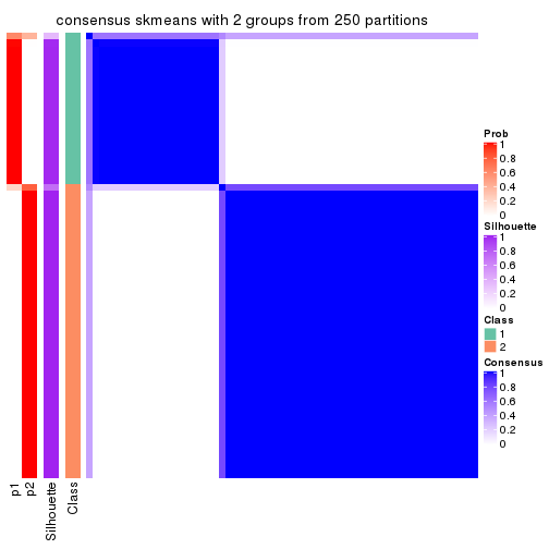
consensus_heatmap(res, k = 3)
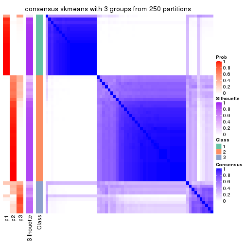
consensus_heatmap(res, k = 4)
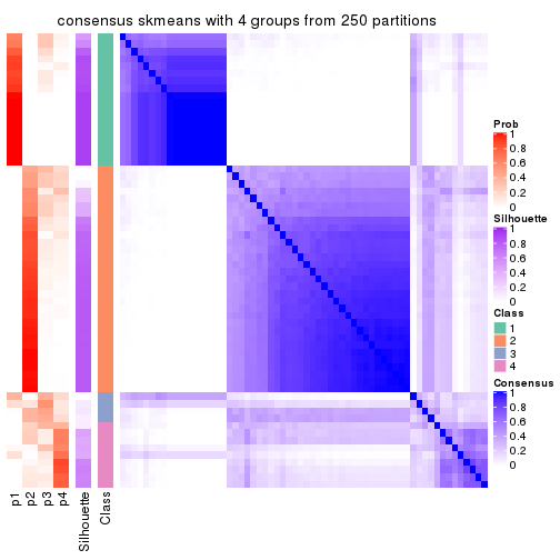
consensus_heatmap(res, k = 5)
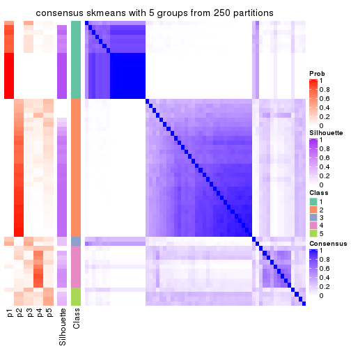
consensus_heatmap(res, k = 6)
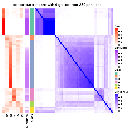
Heatmaps for the membership of samples in all partitions to see how consistent they are:
membership_heatmap(res, k = 2)
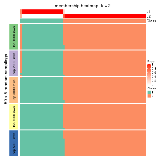
membership_heatmap(res, k = 3)
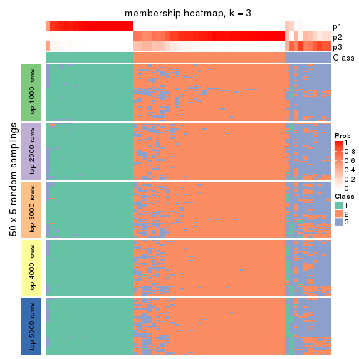
membership_heatmap(res, k = 4)
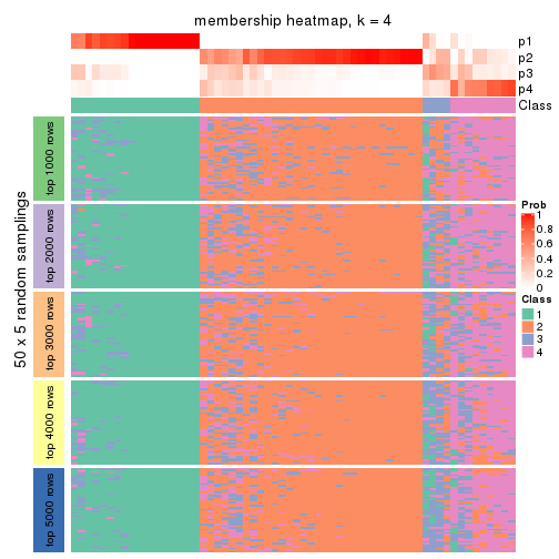
membership_heatmap(res, k = 5)
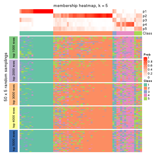
membership_heatmap(res, k = 6)
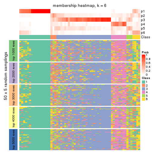
As soon as we have had the classes for columns, we can look for signatures which are significantly different between classes which can be candidate marks for certain classes. Following are the heatmaps for signatures.
Signature heatmaps where rows are scaled:
get_signatures(res, k = 2)
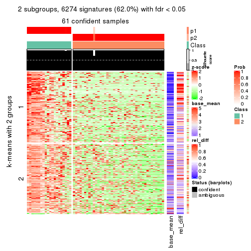
get_signatures(res, k = 3)
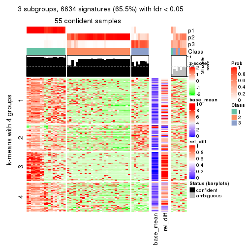
get_signatures(res, k = 4)
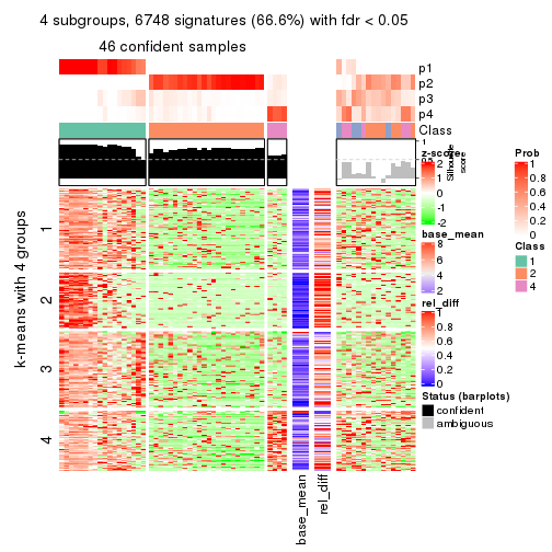
get_signatures(res, k = 5)
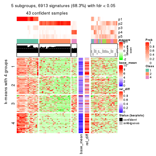
get_signatures(res, k = 6)
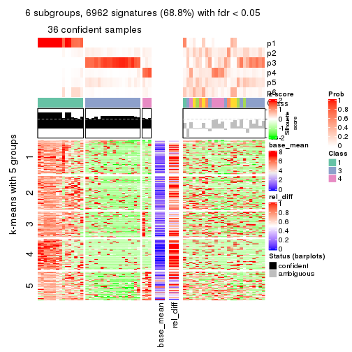
Signature heatmaps where rows are not scaled:
get_signatures(res, k = 2, scale_rows = FALSE)
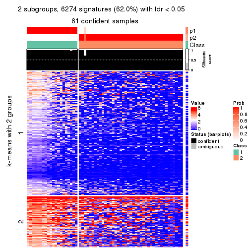
get_signatures(res, k = 3, scale_rows = FALSE)
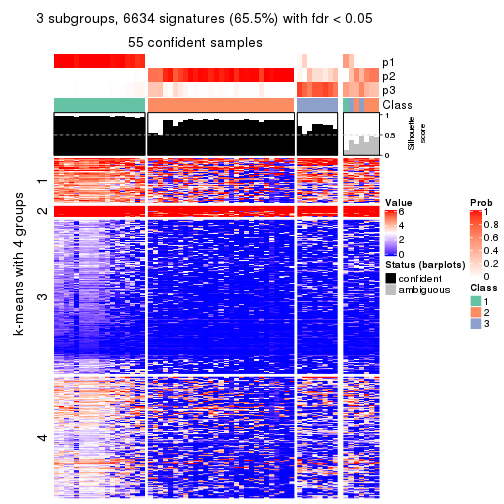
get_signatures(res, k = 4, scale_rows = FALSE)
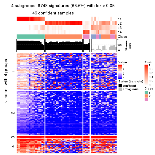
get_signatures(res, k = 5, scale_rows = FALSE)
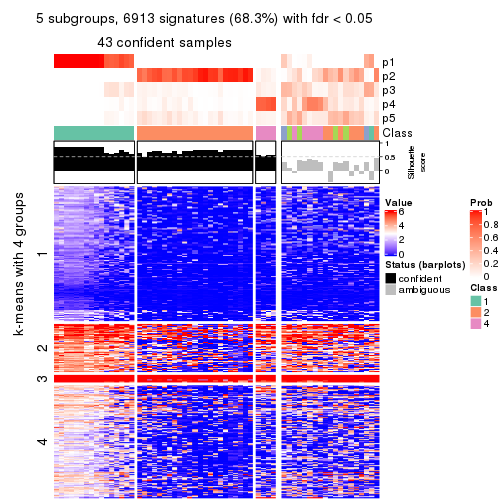
get_signatures(res, k = 6, scale_rows = FALSE)
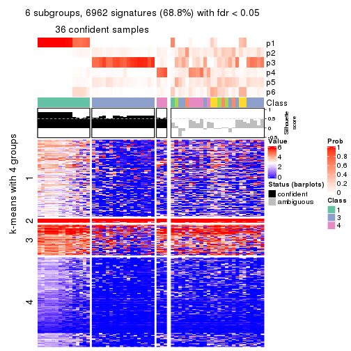
Compare the overlap of signatures from different k:
compare_signatures(res)
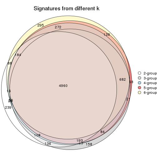
get_signature() returns a data frame invisibly. TO get the list of signatures, the function
call should be assigned to a variable explicitly. In following code, if plot argument is set
to FALSE, no heatmap is plotted while only the differential analysis is performed.
# code only for demonstration
tb = get_signature(res, k = ..., plot = FALSE)
An example of the output of tb is:
#>   which_row         fdr    mean_1    mean_2 scaled_mean_1 scaled_mean_2 km
#> 1        38 0.042760348  8.373488  9.131774    -0.5533452     0.5164555  1
#> 2        40 0.018707592  7.106213  8.469186    -0.6173731     0.5762149  1
#> 3        55 0.019134737 10.221463 11.207825    -0.6159697     0.5749050  1
#> 4        59 0.006059896  5.921854  7.869574    -0.6899429     0.6439467  1
#> 5        60 0.018055526  8.928898 10.211722    -0.6204761     0.5791110  1
#> 6        98 0.009384629 15.714769 14.887706     0.6635654    -0.6193277  2
...
The columns in tb are:
which_row: row indices corresponding to the input matrix.fdr: FDR for the differential test. mean_x: The mean value in group x.scaled_mean_x: The mean value in group x after rows are scaled.km: Row groups if k-means clustering is applied to rows.UMAP plot which shows how samples are separated.
dimension_reduction(res, k = 2, method = "UMAP")
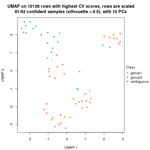
dimension_reduction(res, k = 3, method = "UMAP")
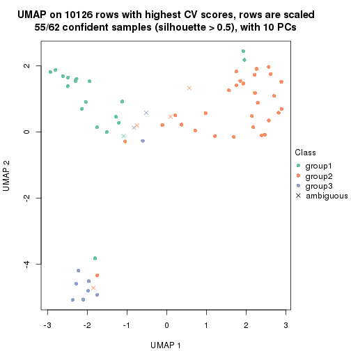
dimension_reduction(res, k = 4, method = "UMAP")
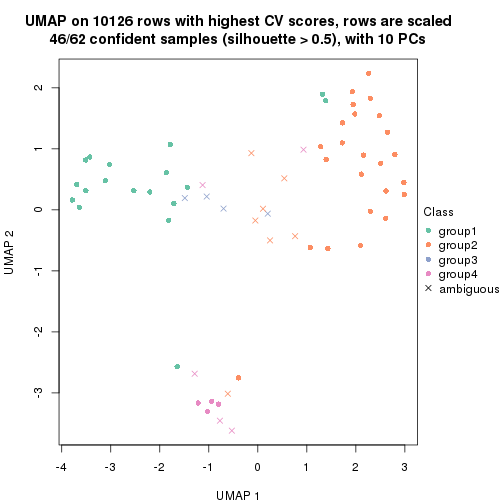
dimension_reduction(res, k = 5, method = "UMAP")

dimension_reduction(res, k = 6, method = "UMAP")
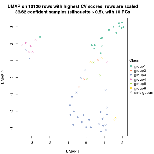
Following heatmap shows how subgroups are split when increasing k:
collect_classes(res)
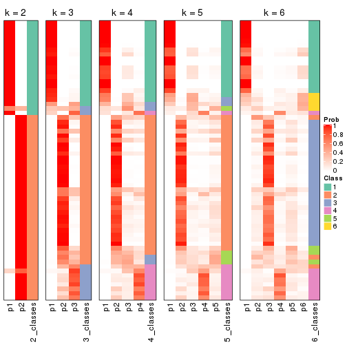
If matrix rows can be associated to genes, consider to use functional_enrichment(res,
...) to perform function enrichment for the signature genes. See this vignette for more detailed explanations.
The object with results only for a single top-value method and a single partition method can be extracted as:
res = res_list["CV", "pam"]
# you can also extract it by
# res = res_list["CV:pam"]
A summary of res and all the functions that can be applied to it:
res
#> A 'ConsensusPartition' object with k = 2, 3, 4, 5, 6.
#>   On a matrix with 10126 rows and 62 columns.
#>   Top rows (1000, 2000, 3000, 4000, 5000) are extracted by 'CV' method.
#>   Subgroups are detected by 'pam' method.
#>   Performed in total 1250 partitions by row resampling.
#>   Best k for subgroups seems to be 2.
#>
#> Following methods can be applied to this 'ConsensusPartition' object:
#>  [1] "cola_report"             "collect_classes"         "collect_plots"
#>  [4] "collect_stats"           "colnames"                "compare_signatures"
#>  [7] "consensus_heatmap"       "dimension_reduction"     "functional_enrichment"
#> [10] "get_anno_col"            "get_anno"                "get_classes"
#> [13] "get_consensus"           "get_matrix"              "get_membership"
#> [16] "get_param"               "get_signatures"          "get_stats"
#> [19] "is_best_k"               "is_stable_k"             "membership_heatmap"
#> [22] "ncol"                    "nrow"                    "plot_ecdf"
#> [25] "rownames"                "select_partition_number" "show"
#> [28] "suggest_best_k"          "test_to_known_factors"
collect_plots() function collects all the plots made from res for all k (number of partitions)
into one single page to provide an easy and fast comparison between different k.
collect_plots(res)
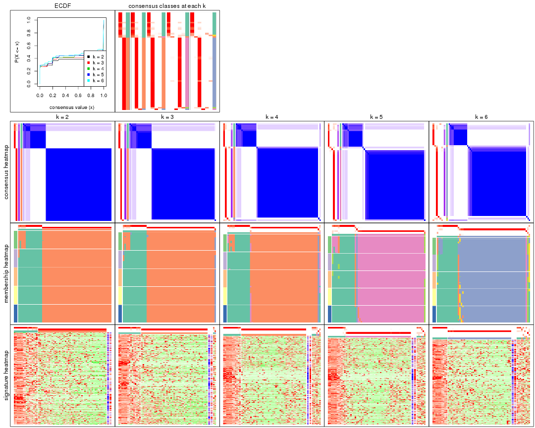
The plots are:
k and the heatmap of
predicted classes for each k.k.k.k.All the plots in panels can be made by individual functions and they are plotted later in this section.
select_partition_number() produces several plots showing different
statistics for choosing “optimized” k. There are following statistics:
k;k, the area increased is defined as \(A_k - A_{k-1}\).The detailed explanations of these statistics can be found in the cola vignette.
Generally speaking, lower PAC score, higher mean silhouette score or higher
concordance corresponds to better partition. Rand index and Jaccard index
measure how similar the current partition is compared to partition with k-1.
If they are too similar, we won't accept k is better than k-1.
select_partition_number(res)
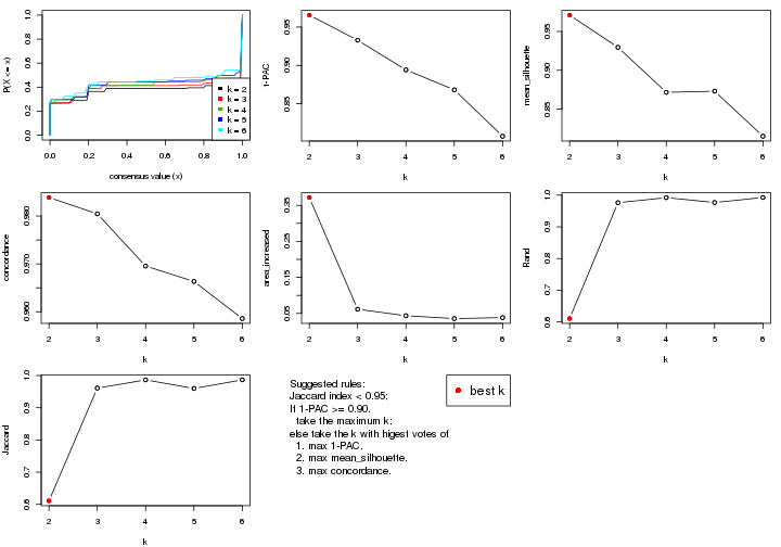
The numeric values for all these statistics can be obtained by get_stats().
get_stats(res)
#>   k 1-PAC mean_silhouette concordance area_increased  Rand Jaccard
#> 2 2 0.966           0.971       0.984         0.3719 0.611   0.611
#> 3 3 0.933           0.930       0.980         0.0616 0.976   0.961
#> 4 4 0.894           0.872       0.970         0.0435 0.992   0.986
#> 5 5 0.868           0.873       0.966         0.0357 0.977   0.960
#> 6 6 0.808           0.815       0.959         0.0383 0.993   0.987
suggest_best_k() suggests the best \(k\) based on these statistics. The rules are as follows:
suggest_best_k(res)
#> [1] 2
Following shows the table of the partitions (You need to click the show/hide
code output link to see it). The membership matrix (columns with name p*)
is inferred by
clue::cl_consensus()
function with the SE method. Basically the value in the membership matrix
represents the probability to belong to a certain group. The finall class
label for an item is determined with the group with highest probability it
belongs to.
In get_classes() function, the entropy is calculated from the membership
matrix and the silhouette score is calculated from the consensus matrix.
cbind(get_classes(res, k = 2), get_membership(res, k = 2))
#>            class entropy silhouette    p1    p2
#> SRR764776      1  0.0000      0.933 1.000 0.000
#> SRR764777      1  0.0000      0.933 1.000 0.000
#> SRR764778      1  0.0000      0.933 1.000 0.000
#> SRR764779      1  0.0000      0.933 1.000 0.000
#> SRR764780      1  0.0000      0.933 1.000 0.000
#> SRR764781      1  0.0000      0.933 1.000 0.000
#> SRR764782      2  0.0000      1.000 0.000 1.000
#> SRR764783      1  0.7219      0.802 0.800 0.200
#> SRR764784      2  0.0000      1.000 0.000 1.000
#> SRR764785      2  0.0000      1.000 0.000 1.000
#> SRR764786      2  0.0000      1.000 0.000 1.000
#> SRR764787      2  0.0000      1.000 0.000 1.000
#> SRR764788      2  0.0000      1.000 0.000 1.000
#> SRR764789      2  0.0000      1.000 0.000 1.000
#> SRR764790      2  0.0000      1.000 0.000 1.000
#> SRR764791      2  0.0000      1.000 0.000 1.000
#> SRR764792      2  0.0000      1.000 0.000 1.000
#> SRR764793      2  0.0000      1.000 0.000 1.000
#> SRR764794      2  0.0000      1.000 0.000 1.000
#> SRR764795      2  0.0000      1.000 0.000 1.000
#> SRR764796      2  0.0000      1.000 0.000 1.000
#> SRR764797      1  0.8713      0.663 0.708 0.292
#> SRR764798      2  0.0000      1.000 0.000 1.000
#> SRR764799      1  0.0000      0.933 1.000 0.000
#> SRR764800      1  0.0000      0.933 1.000 0.000
#> SRR764801      2  0.0376      0.996 0.004 0.996
#> SRR764802      1  0.4939      0.876 0.892 0.108
#> SRR764803      1  0.7139      0.806 0.804 0.196
#> SRR764804      2  0.0000      1.000 0.000 1.000
#> SRR764805      2  0.0000      1.000 0.000 1.000
#> SRR764806      2  0.0000      1.000 0.000 1.000
#> SRR764807      2  0.0000      1.000 0.000 1.000
#> SRR764808      2  0.0000      1.000 0.000 1.000
#> SRR764809      2  0.0000      1.000 0.000 1.000
#> SRR764810      2  0.0000      1.000 0.000 1.000
#> SRR764811      2  0.0000      1.000 0.000 1.000
#> SRR764812      2  0.0000      1.000 0.000 1.000
#> SRR764813      2  0.0000      1.000 0.000 1.000
#> SRR764814      1  0.7219      0.802 0.800 0.200
#> SRR764815      2  0.0000      1.000 0.000 1.000
#> SRR764816      1  0.0000      0.933 1.000 0.000
#> SRR764817      1  0.0000      0.933 1.000 0.000
#> SRR1066622     2  0.0000      1.000 0.000 1.000
#> SRR1066623     2  0.0000      1.000 0.000 1.000
#> SRR1066624     1  0.0000      0.933 1.000 0.000
#> SRR1066625     2  0.0000      1.000 0.000 1.000
#> SRR1066626     2  0.0000      1.000 0.000 1.000
#> SRR1066627     2  0.0000      1.000 0.000 1.000
#> SRR1066628     2  0.0000      1.000 0.000 1.000
#> SRR1066629     2  0.0000      1.000 0.000 1.000
#> SRR1066630     2  0.0000      1.000 0.000 1.000
#> SRR1066631     2  0.0000      1.000 0.000 1.000
#> SRR1066632     2  0.0000      1.000 0.000 1.000
#> SRR1066633     2  0.0000      1.000 0.000 1.000
#> SRR1066634     2  0.0000      1.000 0.000 1.000
#> SRR1066635     2  0.0000      1.000 0.000 1.000
#> SRR1066636     2  0.0000      1.000 0.000 1.000
#> SRR1066637     2  0.0000      1.000 0.000 1.000
#> SRR1066638     2  0.0000      1.000 0.000 1.000
#> SRR1066639     2  0.0000      1.000 0.000 1.000
#> SRR1066640     2  0.0000      1.000 0.000 1.000
#> SRR1066641     2  0.0000      1.000 0.000 1.000
cbind(get_classes(res, k = 3), get_membership(res, k = 3))
#>            class entropy silhouette    p1    p2    p3
#> SRR764776      1   0.000      0.868 1.000 0.000 0.000
#> SRR764777      1   0.000      0.868 1.000 0.000 0.000
#> SRR764778      1   0.000      0.868 1.000 0.000 0.000
#> SRR764779      1   0.000      0.868 1.000 0.000 0.000
#> SRR764780      1   0.000      0.868 1.000 0.000 0.000
#> SRR764781      1   0.000      0.868 1.000 0.000 0.000
#> SRR764782      2   0.000      0.999 0.000 1.000 0.000
#> SRR764783      1   0.455      0.651 0.800 0.200 0.000
#> SRR764784      2   0.000      0.999 0.000 1.000 0.000
#> SRR764785      2   0.000      0.999 0.000 1.000 0.000
#> SRR764786      2   0.000      0.999 0.000 1.000 0.000
#> SRR764787      2   0.000      0.999 0.000 1.000 0.000
#> SRR764788      2   0.000      0.999 0.000 1.000 0.000
#> SRR764789      2   0.000      0.999 0.000 1.000 0.000
#> SRR764790      2   0.000      0.999 0.000 1.000 0.000
#> SRR764791      2   0.000      0.999 0.000 1.000 0.000
#> SRR764792      2   0.000      0.999 0.000 1.000 0.000
#> SRR764793      2   0.000      0.999 0.000 1.000 0.000
#> SRR764794      2   0.000      0.999 0.000 1.000 0.000
#> SRR764795      2   0.000      0.999 0.000 1.000 0.000
#> SRR764796      2   0.000      0.999 0.000 1.000 0.000
#> SRR764797      1   0.712      0.440 0.672 0.272 0.056
#> SRR764798      3   0.327      0.000 0.000 0.116 0.884
#> SRR764799      1   0.000      0.868 1.000 0.000 0.000
#> SRR764800      1   0.000      0.868 1.000 0.000 0.000
#> SRR764801      2   0.116      0.966 0.000 0.972 0.028
#> SRR764802      1   0.319      0.763 0.888 0.112 0.000
#> SRR764803      1   0.450      0.657 0.804 0.196 0.000
#> SRR764804      2   0.000      0.999 0.000 1.000 0.000
#> SRR764805      2   0.000      0.999 0.000 1.000 0.000
#> SRR764806      2   0.000      0.999 0.000 1.000 0.000
#> SRR764807      2   0.000      0.999 0.000 1.000 0.000
#> SRR764808      2   0.000      0.999 0.000 1.000 0.000
#> SRR764809      2   0.000      0.999 0.000 1.000 0.000
#> SRR764810      2   0.000      0.999 0.000 1.000 0.000
#> SRR764811      2   0.000      0.999 0.000 1.000 0.000
#> SRR764812      2   0.000      0.999 0.000 1.000 0.000
#> SRR764813      2   0.000      0.999 0.000 1.000 0.000
#> SRR764814      1   0.478      0.649 0.796 0.200 0.004
#> SRR764815      2   0.000      0.999 0.000 1.000 0.000
#> SRR764816      1   0.000      0.868 1.000 0.000 0.000
#> SRR764817      1   0.000      0.868 1.000 0.000 0.000
#> SRR1066622     2   0.000      0.999 0.000 1.000 0.000
#> SRR1066623     2   0.000      0.999 0.000 1.000 0.000
#> SRR1066624     1   0.116      0.855 0.972 0.000 0.028
#> SRR1066625     2   0.000      0.999 0.000 1.000 0.000
#> SRR1066626     2   0.000      0.999 0.000 1.000 0.000
#> SRR1066627     2   0.000      0.999 0.000 1.000 0.000
#> SRR1066628     2   0.000      0.999 0.000 1.000 0.000
#> SRR1066629     2   0.000      0.999 0.000 1.000 0.000
#> SRR1066630     2   0.000      0.999 0.000 1.000 0.000
#> SRR1066631     2   0.000      0.999 0.000 1.000 0.000
#> SRR1066632     2   0.000      0.999 0.000 1.000 0.000
#> SRR1066633     2   0.000      0.999 0.000 1.000 0.000
#> SRR1066634     2   0.000      0.999 0.000 1.000 0.000
#> SRR1066635     2   0.000      0.999 0.000 1.000 0.000
#> SRR1066636     2   0.000      0.999 0.000 1.000 0.000
#> SRR1066637     2   0.000      0.999 0.000 1.000 0.000
#> SRR1066638     2   0.000      0.999 0.000 1.000 0.000
#> SRR1066639     2   0.000      0.999 0.000 1.000 0.000
#> SRR1066640     2   0.000      0.999 0.000 1.000 0.000
#> SRR1066641     2   0.000      0.999 0.000 1.000 0.000
cbind(get_classes(res, k = 4), get_membership(res, k = 4))
#>            class entropy silhouette    p1    p2    p3    p4
#> SRR764776      1  0.0000     0.8442 1.000 0.000 0.000 0.000
#> SRR764777      1  0.0000     0.8442 1.000 0.000 0.000 0.000
#> SRR764778      1  0.0000     0.8442 1.000 0.000 0.000 0.000
#> SRR764779      1  0.0000     0.8442 1.000 0.000 0.000 0.000
#> SRR764780      1  0.0000     0.8442 1.000 0.000 0.000 0.000
#> SRR764781      1  0.0000     0.8442 1.000 0.000 0.000 0.000
#> SRR764782      2  0.0000     0.9870 0.000 1.000 0.000 0.000
#> SRR764783      1  0.3610     0.2966 0.800 0.200 0.000 0.000
#> SRR764784      2  0.0000     0.9870 0.000 1.000 0.000 0.000
#> SRR764785      2  0.0000     0.9870 0.000 1.000 0.000 0.000
#> SRR764786      2  0.0000     0.9870 0.000 1.000 0.000 0.000
#> SRR764787      2  0.0000     0.9870 0.000 1.000 0.000 0.000
#> SRR764788      2  0.0000     0.9870 0.000 1.000 0.000 0.000
#> SRR764789      2  0.0000     0.9870 0.000 1.000 0.000 0.000
#> SRR764790      2  0.0000     0.9870 0.000 1.000 0.000 0.000
#> SRR764791      2  0.0000     0.9870 0.000 1.000 0.000 0.000
#> SRR764792      2  0.0000     0.9870 0.000 1.000 0.000 0.000
#> SRR764793      2  0.0000     0.9870 0.000 1.000 0.000 0.000
#> SRR764794      2  0.0000     0.9870 0.000 1.000 0.000 0.000
#> SRR764795      2  0.0000     0.9870 0.000 1.000 0.000 0.000
#> SRR764796      2  0.0000     0.9870 0.000 1.000 0.000 0.000
#> SRR764797      4  0.7619     0.0000 0.356 0.208 0.000 0.436
#> SRR764798      3  0.0817     0.0000 0.000 0.024 0.976 0.000
#> SRR764799      1  0.0000     0.8442 1.000 0.000 0.000 0.000
#> SRR764800      1  0.0000     0.8442 1.000 0.000 0.000 0.000
#> SRR764801      2  0.4977    -0.0456 0.000 0.540 0.000 0.460
#> SRR764802      1  0.2589     0.5991 0.884 0.116 0.000 0.000
#> SRR764803      1  0.3569     0.3151 0.804 0.196 0.000 0.000
#> SRR764804      2  0.0000     0.9870 0.000 1.000 0.000 0.000
#> SRR764805      2  0.0000     0.9870 0.000 1.000 0.000 0.000
#> SRR764806      2  0.0000     0.9870 0.000 1.000 0.000 0.000
#> SRR764807      2  0.0000     0.9870 0.000 1.000 0.000 0.000
#> SRR764808      2  0.0000     0.9870 0.000 1.000 0.000 0.000
#> SRR764809      2  0.0000     0.9870 0.000 1.000 0.000 0.000
#> SRR764810      2  0.0000     0.9870 0.000 1.000 0.000 0.000
#> SRR764811      2  0.0000     0.9870 0.000 1.000 0.000 0.000
#> SRR764812      2  0.0000     0.9870 0.000 1.000 0.000 0.000
#> SRR764813      2  0.0000     0.9870 0.000 1.000 0.000 0.000
#> SRR764814      1  0.4240     0.2639 0.784 0.200 0.004 0.012
#> SRR764815      2  0.0000     0.9870 0.000 1.000 0.000 0.000
#> SRR764816      1  0.0000     0.8442 1.000 0.000 0.000 0.000
#> SRR764817      1  0.0000     0.8442 1.000 0.000 0.000 0.000
#> SRR1066622     2  0.0000     0.9870 0.000 1.000 0.000 0.000
#> SRR1066623     2  0.0000     0.9870 0.000 1.000 0.000 0.000
#> SRR1066624     1  0.2775     0.7490 0.896 0.000 0.020 0.084
#> SRR1066625     2  0.0336     0.9777 0.000 0.992 0.000 0.008
#> SRR1066626     2  0.0000     0.9870 0.000 1.000 0.000 0.000
#> SRR1066627     2  0.0000     0.9870 0.000 1.000 0.000 0.000
#> SRR1066628     2  0.0000     0.9870 0.000 1.000 0.000 0.000
#> SRR1066629     2  0.0000     0.9870 0.000 1.000 0.000 0.000
#> SRR1066630     2  0.0000     0.9870 0.000 1.000 0.000 0.000
#> SRR1066631     2  0.0000     0.9870 0.000 1.000 0.000 0.000
#> SRR1066632     2  0.0000     0.9870 0.000 1.000 0.000 0.000
#> SRR1066633     2  0.0000     0.9870 0.000 1.000 0.000 0.000
#> SRR1066634     2  0.0000     0.9870 0.000 1.000 0.000 0.000
#> SRR1066635     2  0.0000     0.9870 0.000 1.000 0.000 0.000
#> SRR1066636     2  0.0000     0.9870 0.000 1.000 0.000 0.000
#> SRR1066637     2  0.0000     0.9870 0.000 1.000 0.000 0.000
#> SRR1066638     2  0.0000     0.9870 0.000 1.000 0.000 0.000
#> SRR1066639     2  0.0000     0.9870 0.000 1.000 0.000 0.000
#> SRR1066640     2  0.0000     0.9870 0.000 1.000 0.000 0.000
#> SRR1066641     2  0.0000     0.9870 0.000 1.000 0.000 0.000
cbind(get_classes(res, k = 5), get_membership(res, k = 5))
#>            class entropy silhouette    p1    p2    p3    p4    p5
#> SRR764776      1  0.0000      0.847 1.000 0.000 0.000 0.000 0.000
#> SRR764777      1  0.0000      0.847 1.000 0.000 0.000 0.000 0.000
#> SRR764778      1  0.0000      0.847 1.000 0.000 0.000 0.000 0.000
#> SRR764779      1  0.0000      0.847 1.000 0.000 0.000 0.000 0.000
#> SRR764780      1  0.0000      0.847 1.000 0.000 0.000 0.000 0.000
#> SRR764781      1  0.0000      0.847 1.000 0.000 0.000 0.000 0.000
#> SRR764782      4  0.0000      0.993 0.000 0.000 0.000 1.000 0.000
#> SRR764783      1  0.3109      0.463 0.800 0.000 0.000 0.200 0.000
#> SRR764784      4  0.0000      0.993 0.000 0.000 0.000 1.000 0.000
#> SRR764785      4  0.0000      0.993 0.000 0.000 0.000 1.000 0.000
#> SRR764786      4  0.0000      0.993 0.000 0.000 0.000 1.000 0.000
#> SRR764787      4  0.0000      0.993 0.000 0.000 0.000 1.000 0.000
#> SRR764788      4  0.0000      0.993 0.000 0.000 0.000 1.000 0.000
#> SRR764789      4  0.0000      0.993 0.000 0.000 0.000 1.000 0.000
#> SRR764790      4  0.0000      0.993 0.000 0.000 0.000 1.000 0.000
#> SRR764791      4  0.0000      0.993 0.000 0.000 0.000 1.000 0.000
#> SRR764792      4  0.0000      0.993 0.000 0.000 0.000 1.000 0.000
#> SRR764793      4  0.0000      0.993 0.000 0.000 0.000 1.000 0.000
#> SRR764794      4  0.0000      0.993 0.000 0.000 0.000 1.000 0.000
#> SRR764795      4  0.1124      0.939 0.000 0.036 0.000 0.960 0.004
#> SRR764796      4  0.0609      0.967 0.000 0.020 0.000 0.980 0.000
#> SRR764797      2  0.5790      0.000 0.184 0.616 0.000 0.200 0.000
#> SRR764798      3  0.0162      0.000 0.000 0.000 0.996 0.004 0.000
#> SRR764799      1  0.0000      0.847 1.000 0.000 0.000 0.000 0.000
#> SRR764800      1  0.0000      0.847 1.000 0.000 0.000 0.000 0.000
#> SRR764801      5  0.3796      0.000 0.000 0.000 0.000 0.300 0.700
#> SRR764802      1  0.2329      0.653 0.876 0.000 0.000 0.124 0.000
#> SRR764803      1  0.3074      0.475 0.804 0.000 0.000 0.196 0.000
#> SRR764804      4  0.0000      0.993 0.000 0.000 0.000 1.000 0.000
#> SRR764805      4  0.0000      0.993 0.000 0.000 0.000 1.000 0.000
#> SRR764806      4  0.0000      0.993 0.000 0.000 0.000 1.000 0.000
#> SRR764807      4  0.0000      0.993 0.000 0.000 0.000 1.000 0.000
#> SRR764808      4  0.0000      0.993 0.000 0.000 0.000 1.000 0.000
#> SRR764809      4  0.0000      0.993 0.000 0.000 0.000 1.000 0.000
#> SRR764810      4  0.0000      0.993 0.000 0.000 0.000 1.000 0.000
#> SRR764811      4  0.0000      0.993 0.000 0.000 0.000 1.000 0.000
#> SRR764812      4  0.0000      0.993 0.000 0.000 0.000 1.000 0.000
#> SRR764813      4  0.0000      0.993 0.000 0.000 0.000 1.000 0.000
#> SRR764814      1  0.5792      0.126 0.616 0.000 0.000 0.192 0.192
#> SRR764815      4  0.0000      0.993 0.000 0.000 0.000 1.000 0.000
#> SRR764816      1  0.0000      0.847 1.000 0.000 0.000 0.000 0.000
#> SRR764817      1  0.0000      0.847 1.000 0.000 0.000 0.000 0.000
#> SRR1066622     4  0.0000      0.993 0.000 0.000 0.000 1.000 0.000
#> SRR1066623     4  0.0000      0.993 0.000 0.000 0.000 1.000 0.000
#> SRR1066624     1  0.5036      0.548 0.704 0.200 0.004 0.000 0.092
#> SRR1066625     4  0.2771      0.759 0.000 0.128 0.000 0.860 0.012
#> SRR1066626     4  0.0000      0.993 0.000 0.000 0.000 1.000 0.000
#> SRR1066627     4  0.0000      0.993 0.000 0.000 0.000 1.000 0.000
#> SRR1066628     4  0.0000      0.993 0.000 0.000 0.000 1.000 0.000
#> SRR1066629     4  0.0000      0.993 0.000 0.000 0.000 1.000 0.000
#> SRR1066630     4  0.0000      0.993 0.000 0.000 0.000 1.000 0.000
#> SRR1066631     4  0.0000      0.993 0.000 0.000 0.000 1.000 0.000
#> SRR1066632     4  0.0000      0.993 0.000 0.000 0.000 1.000 0.000
#> SRR1066633     4  0.0000      0.993 0.000 0.000 0.000 1.000 0.000
#> SRR1066634     4  0.0000      0.993 0.000 0.000 0.000 1.000 0.000
#> SRR1066635     4  0.0000      0.993 0.000 0.000 0.000 1.000 0.000
#> SRR1066636     4  0.0000      0.993 0.000 0.000 0.000 1.000 0.000
#> SRR1066637     4  0.0000      0.993 0.000 0.000 0.000 1.000 0.000
#> SRR1066638     4  0.0000      0.993 0.000 0.000 0.000 1.000 0.000
#> SRR1066639     4  0.0000      0.993 0.000 0.000 0.000 1.000 0.000
#> SRR1066640     4  0.0000      0.993 0.000 0.000 0.000 1.000 0.000
#> SRR1066641     4  0.0000      0.993 0.000 0.000 0.000 1.000 0.000
cbind(get_classes(res, k = 6), get_membership(res, k = 6))
#>            class entropy silhouette    p1    p2    p3 p4    p5    p6
#> SRR764776      1   0.000      0.786 1.000 0.000 0.000  0 0.000 0.000
#> SRR764777      1   0.000      0.786 1.000 0.000 0.000  0 0.000 0.000
#> SRR764778      1   0.000      0.786 1.000 0.000 0.000  0 0.000 0.000
#> SRR764779      1   0.000      0.786 1.000 0.000 0.000  0 0.000 0.000
#> SRR764780      1   0.000      0.786 1.000 0.000 0.000  0 0.000 0.000
#> SRR764781      1   0.000      0.786 1.000 0.000 0.000  0 0.000 0.000
#> SRR764782      3   0.000      0.983 0.000 0.000 1.000  0 0.000 0.000
#> SRR764783      1   0.279      0.222 0.800 0.000 0.200  0 0.000 0.000
#> SRR764784      3   0.000      0.983 0.000 0.000 1.000  0 0.000 0.000
#> SRR764785      3   0.000      0.983 0.000 0.000 1.000  0 0.000 0.000
#> SRR764786      3   0.000      0.983 0.000 0.000 1.000  0 0.000 0.000
#> SRR764787      3   0.000      0.983 0.000 0.000 1.000  0 0.000 0.000
#> SRR764788      3   0.000      0.983 0.000 0.000 1.000  0 0.000 0.000
#> SRR764789      3   0.000      0.983 0.000 0.000 1.000  0 0.000 0.000
#> SRR764790      3   0.000      0.983 0.000 0.000 1.000  0 0.000 0.000
#> SRR764791      3   0.000      0.983 0.000 0.000 1.000  0 0.000 0.000
#> SRR764792      3   0.000      0.983 0.000 0.000 1.000  0 0.000 0.000
#> SRR764793      3   0.000      0.983 0.000 0.000 1.000  0 0.000 0.000
#> SRR764794      3   0.000      0.983 0.000 0.000 1.000  0 0.000 0.000
#> SRR764795      3   0.226      0.839 0.000 0.056 0.896  0 0.000 0.048
#> SRR764796      3   0.195      0.858 0.000 0.016 0.908  0 0.000 0.076
#> SRR764797      2   0.402      0.000 0.072 0.744 0.184  0 0.000 0.000
#> SRR764798      4   0.000      0.000 0.000 0.000 0.000  1 0.000 0.000
#> SRR764799      1   0.000      0.786 1.000 0.000 0.000  0 0.000 0.000
#> SRR764800      1   0.000      0.786 1.000 0.000 0.000  0 0.000 0.000
#> SRR764801      5   0.545      0.000 0.000 0.180 0.252  0 0.568 0.000
#> SRR764802      1   0.209      0.454 0.876 0.000 0.124  0 0.000 0.000
#> SRR764803      1   0.295      0.248 0.804 0.000 0.188  0 0.000 0.008
#> SRR764804      3   0.000      0.983 0.000 0.000 1.000  0 0.000 0.000
#> SRR764805      3   0.000      0.983 0.000 0.000 1.000  0 0.000 0.000
#> SRR764806      3   0.000      0.983 0.000 0.000 1.000  0 0.000 0.000
#> SRR764807      3   0.000      0.983 0.000 0.000 1.000  0 0.000 0.000
#> SRR764808      3   0.000      0.983 0.000 0.000 1.000  0 0.000 0.000
#> SRR764809      3   0.000      0.983 0.000 0.000 1.000  0 0.000 0.000
#> SRR764810      3   0.000      0.983 0.000 0.000 1.000  0 0.000 0.000
#> SRR764811      3   0.000      0.983 0.000 0.000 1.000  0 0.000 0.000
#> SRR764812      3   0.000      0.983 0.000 0.000 1.000  0 0.000 0.000
#> SRR764813      3   0.000      0.983 0.000 0.000 1.000  0 0.000 0.000
#> SRR764814      6   0.494      0.000 0.448 0.000 0.064  0 0.000 0.488
#> SRR764815      3   0.000      0.983 0.000 0.000 1.000  0 0.000 0.000
#> SRR764816      1   0.000      0.786 1.000 0.000 0.000  0 0.000 0.000
#> SRR764817      1   0.000      0.786 1.000 0.000 0.000  0 0.000 0.000
#> SRR1066622     3   0.000      0.983 0.000 0.000 1.000  0 0.000 0.000
#> SRR1066623     3   0.000      0.983 0.000 0.000 1.000  0 0.000 0.000
#> SRR1066624     1   0.456     -0.408 0.540 0.000 0.000  0 0.424 0.036
#> SRR1066625     3   0.397      0.163 0.000 0.004 0.644  0 0.008 0.344
#> SRR1066626     3   0.000      0.983 0.000 0.000 1.000  0 0.000 0.000
#> SRR1066627     3   0.000      0.983 0.000 0.000 1.000  0 0.000 0.000
#> SRR1066628     3   0.000      0.983 0.000 0.000 1.000  0 0.000 0.000
#> SRR1066629     3   0.000      0.983 0.000 0.000 1.000  0 0.000 0.000
#> SRR1066630     3   0.000      0.983 0.000 0.000 1.000  0 0.000 0.000
#> SRR1066631     3   0.000      0.983 0.000 0.000 1.000  0 0.000 0.000
#> SRR1066632     3   0.000      0.983 0.000 0.000 1.000  0 0.000 0.000
#> SRR1066633     3   0.000      0.983 0.000 0.000 1.000  0 0.000 0.000
#> SRR1066634     3   0.000      0.983 0.000 0.000 1.000  0 0.000 0.000
#> SRR1066635     3   0.000      0.983 0.000 0.000 1.000  0 0.000 0.000
#> SRR1066636     3   0.000      0.983 0.000 0.000 1.000  0 0.000 0.000
#> SRR1066637     3   0.000      0.983 0.000 0.000 1.000  0 0.000 0.000
#> SRR1066638     3   0.000      0.983 0.000 0.000 1.000  0 0.000 0.000
#> SRR1066639     3   0.000      0.983 0.000 0.000 1.000  0 0.000 0.000
#> SRR1066640     3   0.000      0.983 0.000 0.000 1.000  0 0.000 0.000
#> SRR1066641     3   0.000      0.983 0.000 0.000 1.000  0 0.000 0.000
Heatmaps for the consensus matrix. It visualizes the probability of two samples to be in a same group.
consensus_heatmap(res, k = 2)
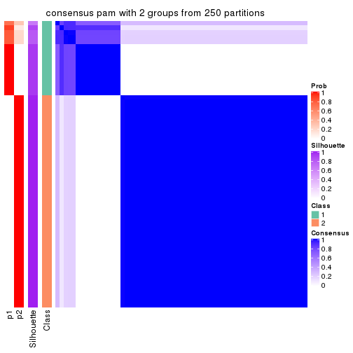
consensus_heatmap(res, k = 3)
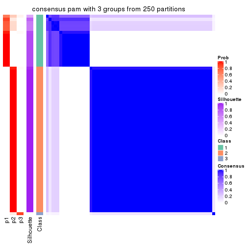
consensus_heatmap(res, k = 4)
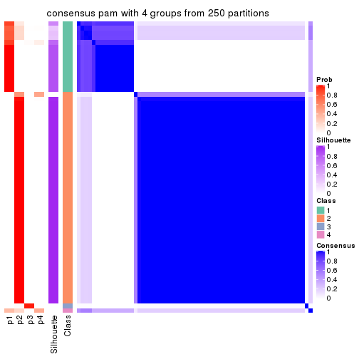
consensus_heatmap(res, k = 5)
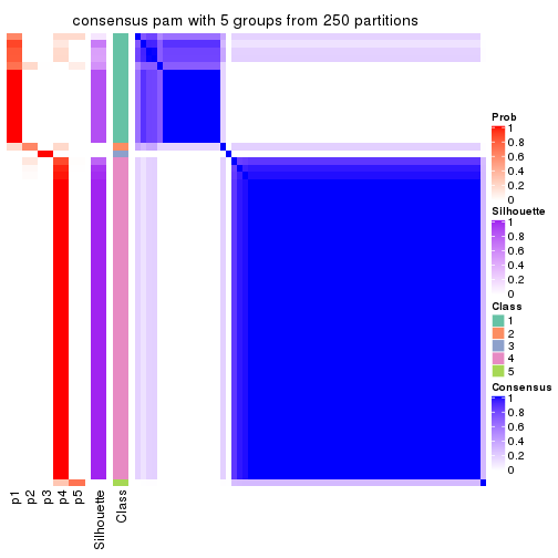
consensus_heatmap(res, k = 6)
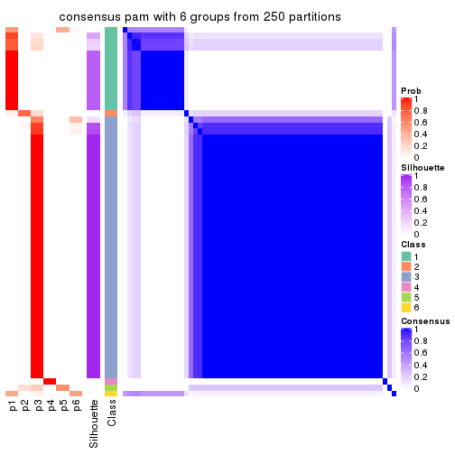
Heatmaps for the membership of samples in all partitions to see how consistent they are:
membership_heatmap(res, k = 2)
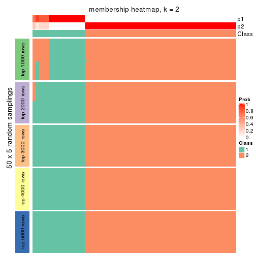
membership_heatmap(res, k = 3)
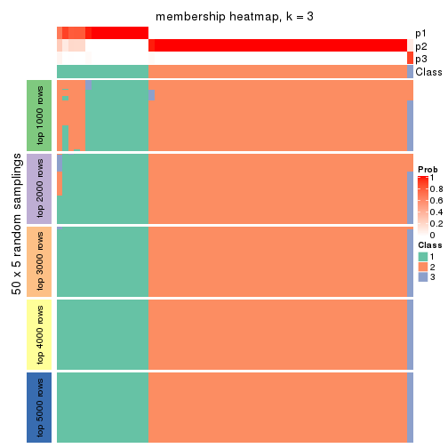
membership_heatmap(res, k = 4)
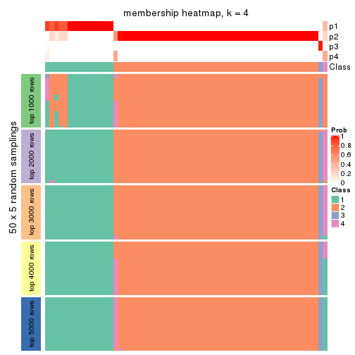
membership_heatmap(res, k = 5)
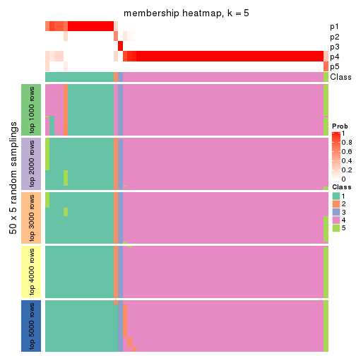
membership_heatmap(res, k = 6)
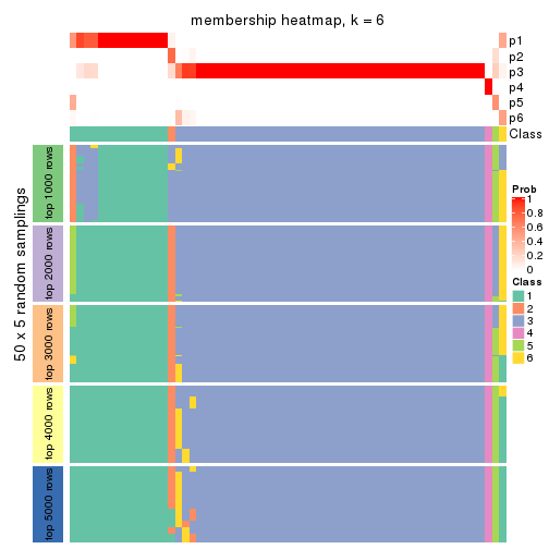
As soon as we have had the classes for columns, we can look for signatures which are significantly different between classes which can be candidate marks for certain classes. Following are the heatmaps for signatures.
Signature heatmaps where rows are scaled:
get_signatures(res, k = 2)
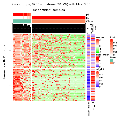
get_signatures(res, k = 3)
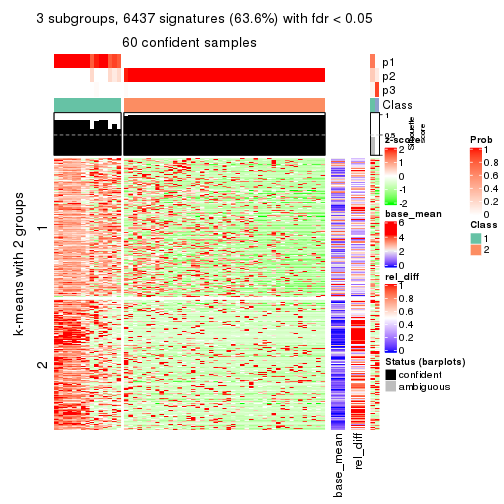
get_signatures(res, k = 4)

get_signatures(res, k = 5)
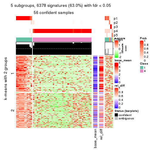
get_signatures(res, k = 6)
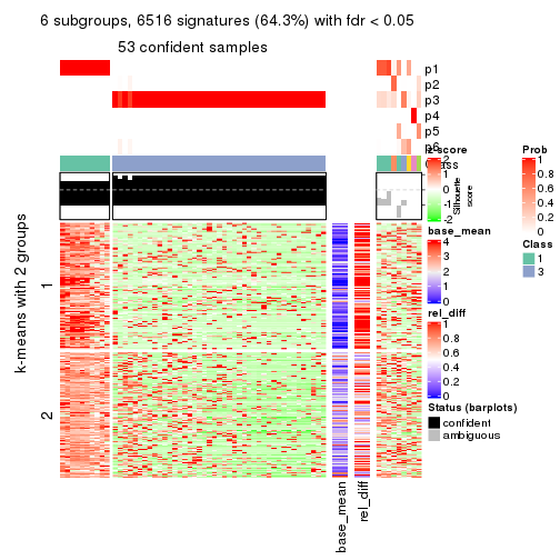
Signature heatmaps where rows are not scaled:
get_signatures(res, k = 2, scale_rows = FALSE)
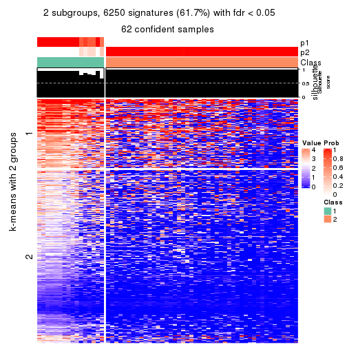
get_signatures(res, k = 3, scale_rows = FALSE)
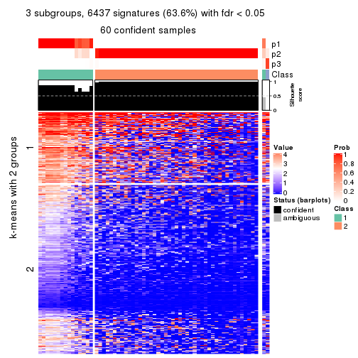
get_signatures(res, k = 4, scale_rows = FALSE)
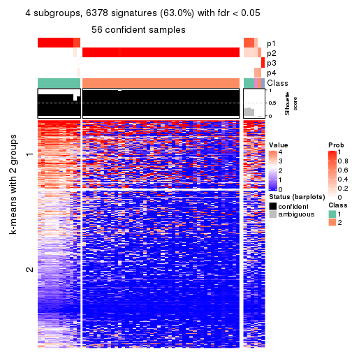
get_signatures(res, k = 5, scale_rows = FALSE)
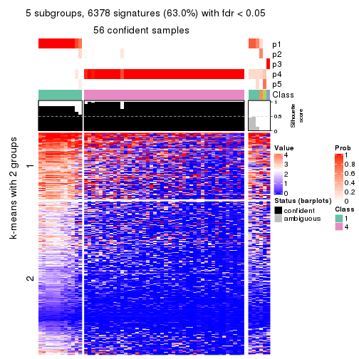
get_signatures(res, k = 6, scale_rows = FALSE)
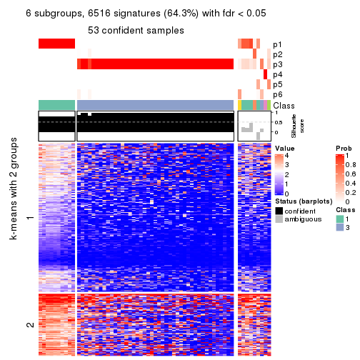
Compare the overlap of signatures from different k:
compare_signatures(res)
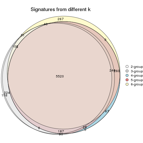
get_signature() returns a data frame invisibly. TO get the list of signatures, the function
call should be assigned to a variable explicitly. In following code, if plot argument is set
to FALSE, no heatmap is plotted while only the differential analysis is performed.
# code only for demonstration
tb = get_signature(res, k = ..., plot = FALSE)
An example of the output of tb is:
#>   which_row         fdr    mean_1    mean_2 scaled_mean_1 scaled_mean_2 km
#> 1        38 0.042760348  8.373488  9.131774    -0.5533452     0.5164555  1
#> 2        40 0.018707592  7.106213  8.469186    -0.6173731     0.5762149  1
#> 3        55 0.019134737 10.221463 11.207825    -0.6159697     0.5749050  1
#> 4        59 0.006059896  5.921854  7.869574    -0.6899429     0.6439467  1
#> 5        60 0.018055526  8.928898 10.211722    -0.6204761     0.5791110  1
#> 6        98 0.009384629 15.714769 14.887706     0.6635654    -0.6193277  2
...
The columns in tb are:
which_row: row indices corresponding to the input matrix.fdr: FDR for the differential test. mean_x: The mean value in group x.scaled_mean_x: The mean value in group x after rows are scaled.km: Row groups if k-means clustering is applied to rows.UMAP plot which shows how samples are separated.
dimension_reduction(res, k = 2, method = "UMAP")
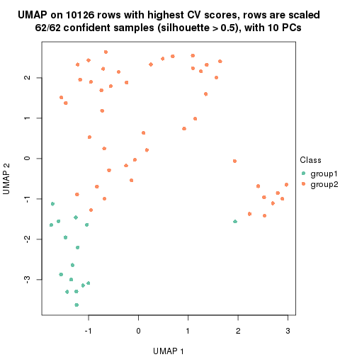
dimension_reduction(res, k = 3, method = "UMAP")
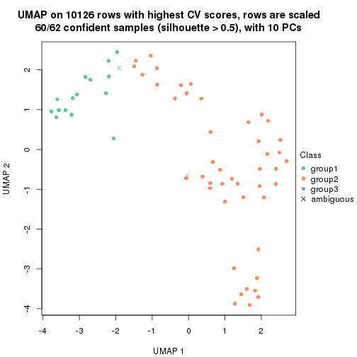
dimension_reduction(res, k = 4, method = "UMAP")
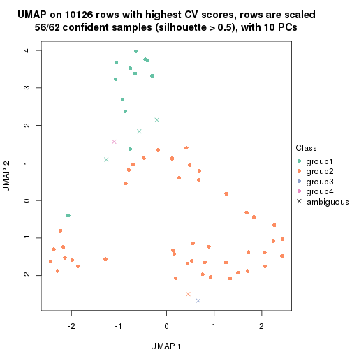
dimension_reduction(res, k = 5, method = "UMAP")
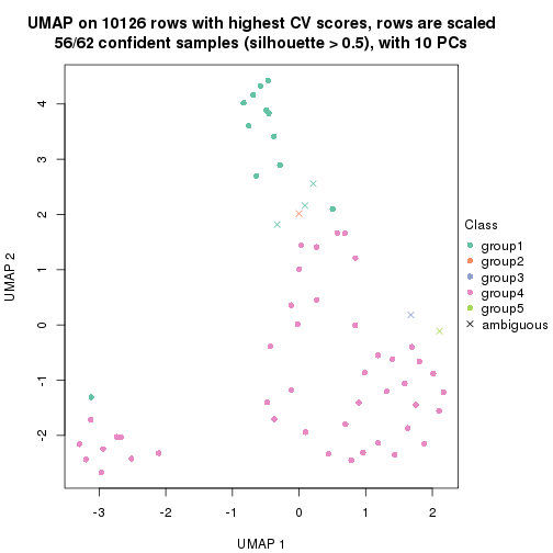
dimension_reduction(res, k = 6, method = "UMAP")
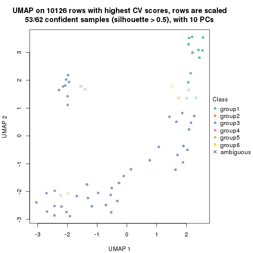
Following heatmap shows how subgroups are split when increasing k:
collect_classes(res)
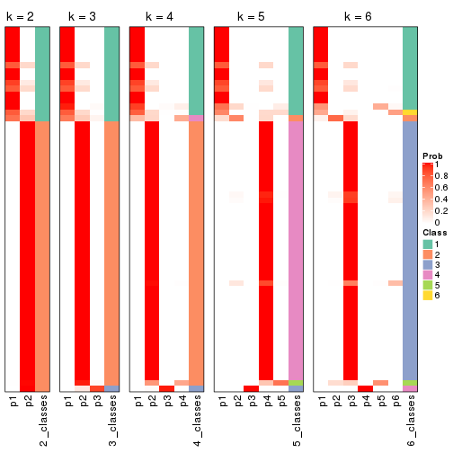
If matrix rows can be associated to genes, consider to use functional_enrichment(res,
...) to perform function enrichment for the signature genes. See this vignette for more detailed explanations.
The object with results only for a single top-value method and a single partition method can be extracted as:
res = res_list["CV", "mclust"]
# you can also extract it by
# res = res_list["CV:mclust"]
A summary of res and all the functions that can be applied to it:
res
#> A 'ConsensusPartition' object with k = 2, 3, 4, 5, 6.
#>   On a matrix with 10126 rows and 62 columns.
#>   Top rows (1000, 2000, 3000, 4000, 5000) are extracted by 'CV' method.
#>   Subgroups are detected by 'mclust' method.
#>   Performed in total 1250 partitions by row resampling.
#>   Best k for subgroups seems to be 2.
#>
#> Following methods can be applied to this 'ConsensusPartition' object:
#>  [1] "cola_report"             "collect_classes"         "collect_plots"
#>  [4] "collect_stats"           "colnames"                "compare_signatures"
#>  [7] "consensus_heatmap"       "dimension_reduction"     "functional_enrichment"
#> [10] "get_anno_col"            "get_anno"                "get_classes"
#> [13] "get_consensus"           "get_matrix"              "get_membership"
#> [16] "get_param"               "get_signatures"          "get_stats"
#> [19] "is_best_k"               "is_stable_k"             "membership_heatmap"
#> [22] "ncol"                    "nrow"                    "plot_ecdf"
#> [25] "rownames"                "select_partition_number" "show"
#> [28] "suggest_best_k"          "test_to_known_factors"
collect_plots() function collects all the plots made from res for all k (number of partitions)
into one single page to provide an easy and fast comparison between different k.
collect_plots(res)
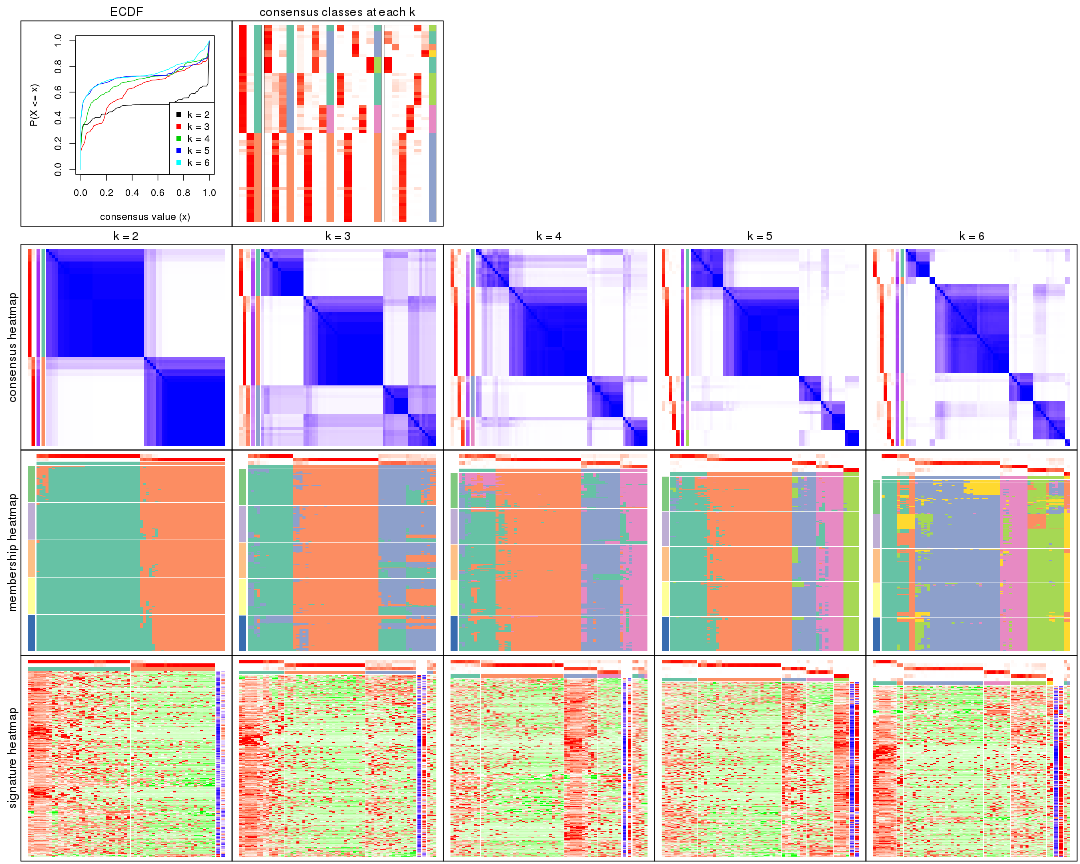
The plots are:
k and the heatmap of
predicted classes for each k.k.k.k.All the plots in panels can be made by individual functions and they are plotted later in this section.
select_partition_number() produces several plots showing different
statistics for choosing “optimized” k. There are following statistics:
k;k, the area increased is defined as \(A_k - A_{k-1}\).The detailed explanations of these statistics can be found in the cola vignette.
Generally speaking, lower PAC score, higher mean silhouette score or higher
concordance corresponds to better partition. Rand index and Jaccard index
measure how similar the current partition is compared to partition with k-1.
If they are too similar, we won't accept k is better than k-1.
select_partition_number(res)
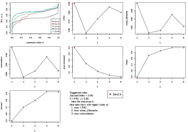
The numeric values for all these statistics can be obtained by get_stats().
get_stats(res)
#>   k 1-PAC mean_silhouette concordance area_increased  Rand Jaccard
#> 2 2 0.901           0.941       0.971         0.4987 0.497   0.497
#> 3 3 0.569           0.769       0.848         0.2409 0.849   0.696
#> 4 4 0.730           0.783       0.873         0.1152 0.928   0.798
#> 5 5 0.862           0.875       0.932         0.0539 0.979   0.928
#> 6 6 0.802           0.808       0.874         0.0268 0.979   0.926
suggest_best_k() suggests the best \(k\) based on these statistics. The rules are as follows:
suggest_best_k(res)
#> [1] 2
Following shows the table of the partitions (You need to click the show/hide
code output link to see it). The membership matrix (columns with name p*)
is inferred by
clue::cl_consensus()
function with the SE method. Basically the value in the membership matrix
represents the probability to belong to a certain group. The finall class
label for an item is determined with the group with highest probability it
belongs to.
In get_classes() function, the entropy is calculated from the membership
matrix and the silhouette score is calculated from the consensus matrix.
cbind(get_classes(res, k = 2), get_membership(res, k = 2))
#>            class entropy silhouette    p1    p2
#> SRR764776      1  0.0000      0.982 1.000 0.000
#> SRR764777      1  0.0000      0.982 1.000 0.000
#> SRR764778      1  0.0000      0.982 1.000 0.000
#> SRR764779      1  0.0000      0.982 1.000 0.000
#> SRR764780      1  0.0000      0.982 1.000 0.000
#> SRR764781      1  0.0000      0.982 1.000 0.000
#> SRR764782      1  0.4939      0.883 0.892 0.108
#> SRR764783      1  0.0000      0.982 1.000 0.000
#> SRR764784      1  0.0938      0.976 0.988 0.012
#> SRR764785      2  0.0000      0.954 0.000 1.000
#> SRR764786      2  0.0000      0.954 0.000 1.000
#> SRR764787      2  0.8443      0.658 0.272 0.728
#> SRR764788      1  0.6247      0.822 0.844 0.156
#> SRR764789      2  0.7453      0.752 0.212 0.788
#> SRR764790      2  0.0000      0.954 0.000 1.000
#> SRR764791      2  0.8144      0.691 0.252 0.748
#> SRR764792      1  0.4298      0.905 0.912 0.088
#> SRR764793      1  0.6148      0.827 0.848 0.152
#> SRR764794      2  0.3879      0.899 0.076 0.924
#> SRR764795      1  0.0000      0.982 1.000 0.000
#> SRR764796      1  0.0376      0.981 0.996 0.004
#> SRR764797      1  0.0000      0.982 1.000 0.000
#> SRR764798      1  0.0000      0.982 1.000 0.000
#> SRR764799      1  0.0000      0.982 1.000 0.000
#> SRR764800      1  0.0000      0.982 1.000 0.000
#> SRR764801      1  0.0000      0.982 1.000 0.000
#> SRR764802      1  0.0000      0.982 1.000 0.000
#> SRR764803      1  0.0000      0.982 1.000 0.000
#> SRR764804      2  0.0000      0.954 0.000 1.000
#> SRR764805      2  0.0000      0.954 0.000 1.000
#> SRR764806      2  0.0376      0.952 0.004 0.996
#> SRR764807      2  0.0000      0.954 0.000 1.000
#> SRR764808      2  0.0000      0.954 0.000 1.000
#> SRR764809      2  0.0000      0.954 0.000 1.000
#> SRR764810      2  0.0000      0.954 0.000 1.000
#> SRR764811      2  0.0000      0.954 0.000 1.000
#> SRR764812      2  0.0000      0.954 0.000 1.000
#> SRR764813      2  0.0000      0.954 0.000 1.000
#> SRR764814      1  0.0000      0.982 1.000 0.000
#> SRR764815      2  0.8955      0.582 0.312 0.688
#> SRR764816      1  0.0000      0.982 1.000 0.000
#> SRR764817      1  0.0000      0.982 1.000 0.000
#> SRR1066622     1  0.0376      0.981 0.996 0.004
#> SRR1066623     1  0.0376      0.981 0.996 0.004
#> SRR1066624     1  0.0376      0.981 0.996 0.004
#> SRR1066625     1  0.0376      0.981 0.996 0.004
#> SRR1066626     1  0.0672      0.979 0.992 0.008
#> SRR1066627     1  0.0376      0.981 0.996 0.004
#> SRR1066628     1  0.0672      0.979 0.992 0.008
#> SRR1066629     1  0.0376      0.981 0.996 0.004
#> SRR1066630     1  0.0938      0.976 0.988 0.012
#> SRR1066631     1  0.0376      0.981 0.996 0.004
#> SRR1066632     2  0.0000      0.954 0.000 1.000
#> SRR1066633     2  0.3274      0.911 0.060 0.940
#> SRR1066634     2  0.0000      0.954 0.000 1.000
#> SRR1066635     2  0.0000      0.954 0.000 1.000
#> SRR1066636     2  0.0000      0.954 0.000 1.000
#> SRR1066637     2  0.0000      0.954 0.000 1.000
#> SRR1066638     2  0.0672      0.950 0.008 0.992
#> SRR1066639     2  0.0000      0.954 0.000 1.000
#> SRR1066640     2  0.0000      0.954 0.000 1.000
#> SRR1066641     2  0.0000      0.954 0.000 1.000
cbind(get_classes(res, k = 3), get_membership(res, k = 3))
#>            class entropy silhouette    p1    p2    p3
#> SRR764776      1  0.0000      0.902 1.000 0.000 0.000
#> SRR764777      1  0.0000      0.902 1.000 0.000 0.000
#> SRR764778      1  0.0000      0.902 1.000 0.000 0.000
#> SRR764779      1  0.0000      0.902 1.000 0.000 0.000
#> SRR764780      1  0.4121      0.782 0.868 0.024 0.108
#> SRR764781      1  0.6986      0.514 0.724 0.096 0.180
#> SRR764782      3  0.8553      0.532 0.112 0.336 0.552
#> SRR764783      3  0.8399      0.622 0.188 0.188 0.624
#> SRR764784      3  0.7860      0.640 0.132 0.204 0.664
#> SRR764785      2  0.0000      0.941 0.000 1.000 0.000
#> SRR764786      2  0.0000      0.941 0.000 1.000 0.000
#> SRR764787      2  0.5591      0.523 0.000 0.696 0.304
#> SRR764788      3  0.8457      0.499 0.100 0.356 0.544
#> SRR764789      2  0.3816      0.794 0.000 0.852 0.148
#> SRR764790      2  0.0237      0.939 0.000 0.996 0.004
#> SRR764791      2  0.4575      0.740 0.004 0.812 0.184
#> SRR764792      3  0.8297      0.525 0.092 0.348 0.560
#> SRR764793      3  0.7918      0.549 0.076 0.328 0.596
#> SRR764794      2  0.5817      0.576 0.020 0.744 0.236
#> SRR764795      3  0.8353      0.619 0.192 0.180 0.628
#> SRR764796      3  0.6982      0.577 0.220 0.072 0.708
#> SRR764797      3  0.9262      0.498 0.324 0.176 0.500
#> SRR764798      1  0.1860      0.881 0.948 0.000 0.052
#> SRR764799      1  0.0000      0.902 1.000 0.000 0.000
#> SRR764800      1  0.0000      0.902 1.000 0.000 0.000
#> SRR764801      1  0.1860      0.881 0.948 0.000 0.052
#> SRR764802      3  0.8440      0.617 0.196 0.184 0.620
#> SRR764803      3  0.8821      0.614 0.232 0.188 0.580
#> SRR764804      2  0.0000      0.941 0.000 1.000 0.000
#> SRR764805      2  0.0000      0.941 0.000 1.000 0.000
#> SRR764806      2  0.0848      0.932 0.008 0.984 0.008
#> SRR764807      2  0.0000      0.941 0.000 1.000 0.000
#> SRR764808      2  0.0000      0.941 0.000 1.000 0.000
#> SRR764809      2  0.0000      0.941 0.000 1.000 0.000
#> SRR764810      2  0.0000      0.941 0.000 1.000 0.000
#> SRR764811      2  0.0000      0.941 0.000 1.000 0.000
#> SRR764812      2  0.0000      0.941 0.000 1.000 0.000
#> SRR764813      2  0.0000      0.941 0.000 1.000 0.000
#> SRR764814      1  0.1267      0.888 0.972 0.004 0.024
#> SRR764815      2  0.6422      0.370 0.016 0.660 0.324
#> SRR764816      1  0.0000      0.902 1.000 0.000 0.000
#> SRR764817      1  0.0000      0.902 1.000 0.000 0.000
#> SRR1066622     3  0.5891      0.557 0.200 0.036 0.764
#> SRR1066623     3  0.5891      0.557 0.200 0.036 0.764
#> SRR1066624     1  0.5465      0.622 0.712 0.000 0.288
#> SRR1066625     1  0.5785      0.541 0.668 0.000 0.332
#> SRR1066626     3  0.6761      0.552 0.252 0.048 0.700
#> SRR1066627     3  0.6187      0.535 0.248 0.028 0.724
#> SRR1066628     3  0.5891      0.557 0.200 0.036 0.764
#> SRR1066629     3  0.5891      0.557 0.200 0.036 0.764
#> SRR1066630     3  0.8914      0.579 0.280 0.164 0.556
#> SRR1066631     3  0.5891      0.557 0.200 0.036 0.764
#> SRR1066632     2  0.0000      0.941 0.000 1.000 0.000
#> SRR1066633     2  0.0848      0.931 0.008 0.984 0.008
#> SRR1066634     2  0.0237      0.939 0.000 0.996 0.004
#> SRR1066635     2  0.0000      0.941 0.000 1.000 0.000
#> SRR1066636     2  0.0237      0.937 0.004 0.996 0.000
#> SRR1066637     2  0.0592      0.933 0.000 0.988 0.012
#> SRR1066638     2  0.0237      0.939 0.000 0.996 0.004
#> SRR1066639     2  0.0000      0.941 0.000 1.000 0.000
#> SRR1066640     2  0.0000      0.941 0.000 1.000 0.000
#> SRR1066641     2  0.0000      0.941 0.000 1.000 0.000
cbind(get_classes(res, k = 4), get_membership(res, k = 4))
#>            class entropy silhouette    p1    p2    p3    p4
#> SRR764776      3  0.2546      0.859 0.060 0.000 0.912 0.028
#> SRR764777      3  0.2546      0.859 0.060 0.000 0.912 0.028
#> SRR764778      3  0.2546      0.859 0.060 0.000 0.912 0.028
#> SRR764779      3  0.2546      0.859 0.060 0.000 0.912 0.028
#> SRR764780      1  0.5679     -0.136 0.492 0.004 0.488 0.016
#> SRR764781      1  0.5349      0.267 0.620 0.008 0.364 0.008
#> SRR764782      1  0.3612      0.704 0.840 0.144 0.004 0.012
#> SRR764783      1  0.2040      0.725 0.936 0.048 0.012 0.004
#> SRR764784      1  0.3081      0.705 0.888 0.064 0.000 0.048
#> SRR764785      2  0.0000      0.947 0.000 1.000 0.000 0.000
#> SRR764786      2  0.0188      0.946 0.000 0.996 0.000 0.004
#> SRR764787      2  0.4642      0.662 0.240 0.740 0.000 0.020
#> SRR764788      1  0.3992      0.673 0.800 0.188 0.004 0.008
#> SRR764789      2  0.3810      0.754 0.188 0.804 0.000 0.008
#> SRR764790      2  0.0592      0.939 0.000 0.984 0.000 0.016
#> SRR764791      2  0.3881      0.765 0.172 0.812 0.000 0.016
#> SRR764792      1  0.5300      0.500 0.664 0.308 0.000 0.028
#> SRR764793      1  0.4872      0.592 0.728 0.244 0.000 0.028
#> SRR764794      2  0.3610      0.750 0.200 0.800 0.000 0.000
#> SRR764795      1  0.2861      0.723 0.908 0.048 0.032 0.012
#> SRR764796      4  0.5666      0.671 0.268 0.012 0.036 0.684
#> SRR764797      1  0.4234      0.671 0.816 0.052 0.132 0.000
#> SRR764798      3  0.3312      0.810 0.072 0.000 0.876 0.052
#> SRR764799      3  0.2670      0.852 0.052 0.000 0.908 0.040
#> SRR764800      3  0.2521      0.860 0.064 0.000 0.912 0.024
#> SRR764801      3  0.3312      0.810 0.072 0.000 0.876 0.052
#> SRR764802      1  0.2075      0.723 0.936 0.044 0.016 0.004
#> SRR764803      1  0.3067      0.691 0.888 0.024 0.084 0.004
#> SRR764804      2  0.0376      0.946 0.004 0.992 0.000 0.004
#> SRR764805      2  0.0188      0.946 0.004 0.996 0.000 0.000
#> SRR764806      2  0.0469      0.943 0.012 0.988 0.000 0.000
#> SRR764807      2  0.0188      0.946 0.000 0.996 0.000 0.004
#> SRR764808      2  0.0188      0.946 0.000 0.996 0.000 0.004
#> SRR764809      2  0.0000      0.947 0.000 1.000 0.000 0.000
#> SRR764810      2  0.0000      0.947 0.000 1.000 0.000 0.000
#> SRR764811      2  0.0000      0.947 0.000 1.000 0.000 0.000
#> SRR764812      2  0.0188      0.946 0.000 0.996 0.000 0.004
#> SRR764813      2  0.0000      0.947 0.000 1.000 0.000 0.000
#> SRR764814      3  0.5306      0.762 0.124 0.068 0.780 0.028
#> SRR764815      2  0.4635      0.622 0.268 0.720 0.000 0.012
#> SRR764816      3  0.1978      0.860 0.068 0.000 0.928 0.004
#> SRR764817      3  0.1902      0.860 0.064 0.000 0.932 0.004
#> SRR1066622     4  0.2197      0.832 0.080 0.004 0.000 0.916
#> SRR1066623     4  0.2125      0.833 0.076 0.004 0.000 0.920
#> SRR1066624     3  0.6091      0.465 0.060 0.000 0.596 0.344
#> SRR1066625     3  0.6186      0.383 0.064 0.000 0.584 0.352
#> SRR1066626     4  0.5568      0.631 0.300 0.008 0.028 0.664
#> SRR1066627     4  0.4906      0.744 0.076 0.004 0.136 0.784
#> SRR1066628     4  0.2266      0.831 0.084 0.004 0.000 0.912
#> SRR1066629     4  0.2125      0.833 0.076 0.004 0.000 0.920
#> SRR1066630     4  0.9575      0.113 0.304 0.224 0.128 0.344
#> SRR1066631     4  0.2125      0.833 0.076 0.004 0.000 0.920
#> SRR1066632     2  0.0000      0.947 0.000 1.000 0.000 0.000
#> SRR1066633     2  0.1637      0.905 0.060 0.940 0.000 0.000
#> SRR1066634     2  0.0188      0.946 0.004 0.996 0.000 0.000
#> SRR1066635     2  0.0524      0.944 0.008 0.988 0.000 0.004
#> SRR1066636     2  0.0000      0.947 0.000 1.000 0.000 0.000
#> SRR1066637     2  0.0336      0.945 0.008 0.992 0.000 0.000
#> SRR1066638     2  0.0376      0.945 0.004 0.992 0.000 0.004
#> SRR1066639     2  0.0336      0.945 0.008 0.992 0.000 0.000
#> SRR1066640     2  0.0000      0.947 0.000 1.000 0.000 0.000
#> SRR1066641     2  0.0188      0.946 0.000 0.996 0.000 0.004
cbind(get_classes(res, k = 5), get_membership(res, k = 5))
#>            class entropy silhouette    p1    p2    p3    p4    p5
#> SRR764776      5  0.0000      0.995 0.000 0.000 0.000 0.000 1.000
#> SRR764777      5  0.0000      0.995 0.000 0.000 0.000 0.000 1.000
#> SRR764778      5  0.0000      0.995 0.000 0.000 0.000 0.000 1.000
#> SRR764779      5  0.0000      0.995 0.000 0.000 0.000 0.000 1.000
#> SRR764780      1  0.2569      0.866 0.892 0.000 0.068 0.000 0.040
#> SRR764781      1  0.1809      0.887 0.928 0.000 0.060 0.000 0.012
#> SRR764782      1  0.2077      0.888 0.908 0.084 0.000 0.008 0.000
#> SRR764783      1  0.0324      0.913 0.992 0.004 0.004 0.000 0.000
#> SRR764784      1  0.1907      0.900 0.928 0.028 0.000 0.044 0.000
#> SRR764785      2  0.0162      0.948 0.004 0.996 0.000 0.000 0.000
#> SRR764786      2  0.0162      0.947 0.004 0.996 0.000 0.000 0.000
#> SRR764787      2  0.4040      0.630 0.276 0.712 0.000 0.012 0.000
#> SRR764788      1  0.2020      0.874 0.900 0.100 0.000 0.000 0.000
#> SRR764789      2  0.3636      0.656 0.272 0.728 0.000 0.000 0.000
#> SRR764790      2  0.0510      0.942 0.016 0.984 0.000 0.000 0.000
#> SRR764791      2  0.3932      0.533 0.328 0.672 0.000 0.000 0.000
#> SRR764792      1  0.2172      0.891 0.908 0.076 0.000 0.016 0.000
#> SRR764793      1  0.2723      0.836 0.864 0.124 0.000 0.012 0.000
#> SRR764794      2  0.1608      0.900 0.072 0.928 0.000 0.000 0.000
#> SRR764795      1  0.0324      0.913 0.992 0.004 0.004 0.000 0.000
#> SRR764796      4  0.3779      0.674 0.236 0.000 0.012 0.752 0.000
#> SRR764797      1  0.2623      0.882 0.888 0.012 0.092 0.004 0.004
#> SRR764798      3  0.0000      0.883 0.000 0.000 1.000 0.000 0.000
#> SRR764799      3  0.1792      0.873 0.000 0.000 0.916 0.000 0.084
#> SRR764800      5  0.0510      0.979 0.000 0.000 0.016 0.000 0.984
#> SRR764801      3  0.0000      0.883 0.000 0.000 1.000 0.000 0.000
#> SRR764802      1  0.0324      0.913 0.992 0.004 0.004 0.000 0.000
#> SRR764803      1  0.0324      0.913 0.992 0.004 0.004 0.000 0.000
#> SRR764804      2  0.0000      0.948 0.000 1.000 0.000 0.000 0.000
#> SRR764805      2  0.0162      0.947 0.004 0.996 0.000 0.000 0.000
#> SRR764806      2  0.0162      0.948 0.004 0.996 0.000 0.000 0.000
#> SRR764807      2  0.0162      0.947 0.004 0.996 0.000 0.000 0.000
#> SRR764808      2  0.0162      0.947 0.004 0.996 0.000 0.000 0.000
#> SRR764809      2  0.0000      0.948 0.000 1.000 0.000 0.000 0.000
#> SRR764810      2  0.0000      0.948 0.000 1.000 0.000 0.000 0.000
#> SRR764811      2  0.0000      0.948 0.000 1.000 0.000 0.000 0.000
#> SRR764812      2  0.0000      0.948 0.000 1.000 0.000 0.000 0.000
#> SRR764813      2  0.0162      0.947 0.004 0.996 0.000 0.000 0.000
#> SRR764814      3  0.3012      0.849 0.072 0.000 0.872 0.004 0.052
#> SRR764815      2  0.3797      0.705 0.232 0.756 0.004 0.008 0.000
#> SRR764816      3  0.3890      0.745 0.012 0.000 0.736 0.000 0.252
#> SRR764817      3  0.4014      0.739 0.016 0.000 0.728 0.000 0.256
#> SRR1066622     4  0.0290      0.838 0.008 0.000 0.000 0.992 0.000
#> SRR1066623     4  0.0162      0.838 0.004 0.000 0.000 0.996 0.000
#> SRR1066624     3  0.0404      0.883 0.000 0.000 0.988 0.012 0.000
#> SRR1066625     3  0.1544      0.857 0.000 0.000 0.932 0.068 0.000
#> SRR1066626     4  0.4323      0.706 0.220 0.012 0.024 0.744 0.000
#> SRR1066627     4  0.3534      0.620 0.000 0.000 0.256 0.744 0.000
#> SRR1066628     4  0.0290      0.838 0.008 0.000 0.000 0.992 0.000
#> SRR1066629     4  0.0162      0.838 0.004 0.000 0.000 0.996 0.000
#> SRR1066630     4  0.6815      0.533 0.192 0.040 0.208 0.560 0.000
#> SRR1066631     4  0.0000      0.836 0.000 0.000 0.000 1.000 0.000
#> SRR1066632     2  0.0162      0.948 0.004 0.996 0.000 0.000 0.000
#> SRR1066633     2  0.1205      0.923 0.040 0.956 0.004 0.000 0.000
#> SRR1066634     2  0.0290      0.947 0.008 0.992 0.000 0.000 0.000
#> SRR1066635     2  0.0162      0.948 0.004 0.996 0.000 0.000 0.000
#> SRR1066636     2  0.0162      0.948 0.004 0.996 0.000 0.000 0.000
#> SRR1066637     2  0.0162      0.948 0.004 0.996 0.000 0.000 0.000
#> SRR1066638     2  0.0162      0.948 0.004 0.996 0.000 0.000 0.000
#> SRR1066639     2  0.0290      0.947 0.008 0.992 0.000 0.000 0.000
#> SRR1066640     2  0.0162      0.948 0.004 0.996 0.000 0.000 0.000
#> SRR1066641     2  0.0000      0.948 0.000 1.000 0.000 0.000 0.000
cbind(get_classes(res, k = 6), get_membership(res, k = 6))
#>            class entropy silhouette    p1    p2    p3    p4    p5    p6
#> SRR764776      1  0.0000      0.785 1.000 0.000 0.000 0.000 0.000 0.000
#> SRR764777      1  0.0000      0.785 1.000 0.000 0.000 0.000 0.000 0.000
#> SRR764778      1  0.0000      0.785 1.000 0.000 0.000 0.000 0.000 0.000
#> SRR764779      1  0.0000      0.785 1.000 0.000 0.000 0.000 0.000 0.000
#> SRR764780      5  0.2171      0.805 0.032 0.016 0.000 0.000 0.912 0.040
#> SRR764781      5  0.1528      0.814 0.000 0.016 0.000 0.000 0.936 0.048
#> SRR764782      5  0.4259      0.797 0.000 0.160 0.096 0.004 0.740 0.000
#> SRR764783      5  0.0260      0.823 0.000 0.000 0.000 0.000 0.992 0.008
#> SRR764784      5  0.4582      0.802 0.000 0.132 0.052 0.068 0.748 0.000
#> SRR764785      3  0.0865      0.889 0.000 0.036 0.964 0.000 0.000 0.000
#> SRR764786      3  0.1152      0.891 0.000 0.044 0.952 0.004 0.000 0.000
#> SRR764787      3  0.5418      0.533 0.000 0.132 0.628 0.020 0.220 0.000
#> SRR764788      5  0.4304      0.794 0.000 0.160 0.100 0.004 0.736 0.000
#> SRR764789      3  0.5362      0.505 0.000 0.200 0.608 0.004 0.188 0.000
#> SRR764790      3  0.2052      0.879 0.000 0.056 0.912 0.028 0.004 0.000
#> SRR764791      3  0.5535      0.400 0.000 0.172 0.572 0.004 0.252 0.000
#> SRR764792      5  0.4886      0.779 0.000 0.188 0.092 0.024 0.696 0.000
#> SRR764793      5  0.4842      0.764 0.000 0.192 0.108 0.012 0.688 0.000
#> SRR764794      3  0.3710      0.774 0.000 0.144 0.788 0.004 0.064 0.000
#> SRR764795      5  0.1109      0.825 0.000 0.012 0.004 0.004 0.964 0.016
#> SRR764796      4  0.3166      0.743 0.000 0.024 0.000 0.816 0.156 0.004
#> SRR764797      5  0.4419      0.791 0.004 0.108 0.016 0.004 0.764 0.104
#> SRR764798      2  0.3547      1.000 0.000 0.668 0.000 0.000 0.000 0.332
#> SRR764799      1  0.4685      0.627 0.664 0.096 0.000 0.000 0.000 0.240
#> SRR764800      1  0.0603      0.782 0.980 0.016 0.000 0.000 0.000 0.004
#> SRR764801      2  0.3547      1.000 0.000 0.668 0.000 0.000 0.000 0.332
#> SRR764802      5  0.0000      0.823 0.000 0.000 0.000 0.000 1.000 0.000
#> SRR764803      5  0.0748      0.829 0.000 0.016 0.004 0.000 0.976 0.004
#> SRR764804      3  0.1349      0.887 0.000 0.056 0.940 0.004 0.000 0.000
#> SRR764805      3  0.1007      0.890 0.000 0.044 0.956 0.000 0.000 0.000
#> SRR764806      3  0.1296      0.889 0.000 0.044 0.948 0.004 0.004 0.000
#> SRR764807      3  0.1204      0.887 0.000 0.056 0.944 0.000 0.000 0.000
#> SRR764808      3  0.1267      0.887 0.000 0.060 0.940 0.000 0.000 0.000
#> SRR764809      3  0.0632      0.892 0.000 0.024 0.976 0.000 0.000 0.000
#> SRR764810      3  0.1493      0.888 0.000 0.056 0.936 0.004 0.004 0.000
#> SRR764811      3  0.1204      0.887 0.000 0.056 0.944 0.000 0.000 0.000
#> SRR764812      3  0.1204      0.887 0.000 0.056 0.944 0.000 0.000 0.000
#> SRR764813      3  0.1267      0.887 0.000 0.060 0.940 0.000 0.000 0.000
#> SRR764814      1  0.7140      0.235 0.456 0.112 0.008 0.008 0.104 0.312
#> SRR764815      3  0.5136      0.600 0.000 0.168 0.660 0.012 0.160 0.000
#> SRR764816      1  0.4486      0.663 0.696 0.096 0.000 0.000 0.000 0.208
#> SRR764817      1  0.4503      0.664 0.696 0.100 0.000 0.000 0.000 0.204
#> SRR1066622     4  0.0146      0.875 0.000 0.000 0.000 0.996 0.004 0.000
#> SRR1066623     4  0.0000      0.876 0.000 0.000 0.000 1.000 0.000 0.000
#> SRR1066624     6  0.0146      0.882 0.000 0.004 0.000 0.000 0.000 0.996
#> SRR1066625     6  0.1075      0.885 0.000 0.000 0.000 0.048 0.000 0.952
#> SRR1066626     4  0.4104      0.738 0.000 0.092 0.028 0.784 0.096 0.000
#> SRR1066627     4  0.1957      0.802 0.000 0.000 0.000 0.888 0.000 0.112
#> SRR1066628     4  0.0000      0.876 0.000 0.000 0.000 1.000 0.000 0.000
#> SRR1066629     4  0.0000      0.876 0.000 0.000 0.000 1.000 0.000 0.000
#> SRR1066630     4  0.5254      0.675 0.000 0.088 0.076 0.724 0.092 0.020
#> SRR1066631     4  0.0000      0.876 0.000 0.000 0.000 1.000 0.000 0.000
#> SRR1066632     3  0.0951      0.893 0.000 0.020 0.968 0.008 0.004 0.000
#> SRR1066633     3  0.2333      0.851 0.000 0.092 0.884 0.000 0.024 0.000
#> SRR1066634     3  0.1349      0.885 0.000 0.056 0.940 0.000 0.004 0.000
#> SRR1066635     3  0.1409      0.889 0.000 0.032 0.948 0.008 0.012 0.000
#> SRR1066636     3  0.0260      0.893 0.000 0.008 0.992 0.000 0.000 0.000
#> SRR1066637     3  0.1007      0.888 0.000 0.044 0.956 0.000 0.000 0.000
#> SRR1066638     3  0.1226      0.889 0.000 0.040 0.952 0.004 0.004 0.000
#> SRR1066639     3  0.1410      0.887 0.000 0.044 0.944 0.004 0.008 0.000
#> SRR1066640     3  0.0547      0.892 0.000 0.020 0.980 0.000 0.000 0.000
#> SRR1066641     3  0.1204      0.887 0.000 0.056 0.944 0.000 0.000 0.000
Heatmaps for the consensus matrix. It visualizes the probability of two samples to be in a same group.
consensus_heatmap(res, k = 2)
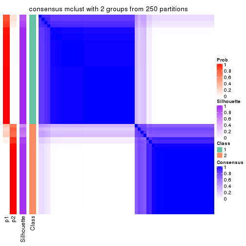
consensus_heatmap(res, k = 3)
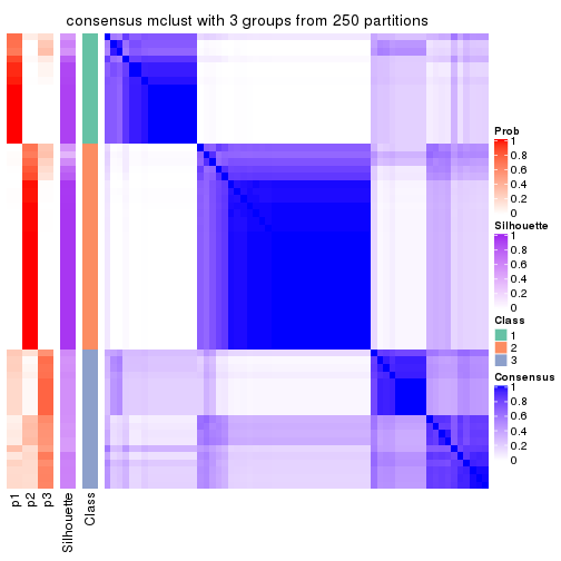
consensus_heatmap(res, k = 4)
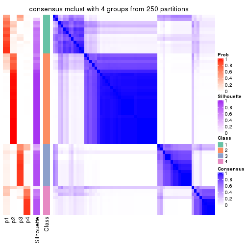
consensus_heatmap(res, k = 5)
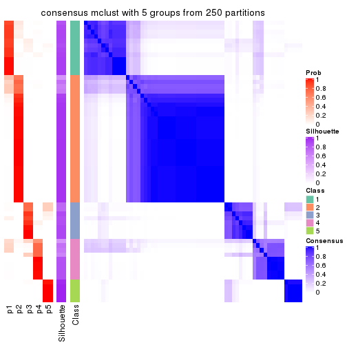
consensus_heatmap(res, k = 6)
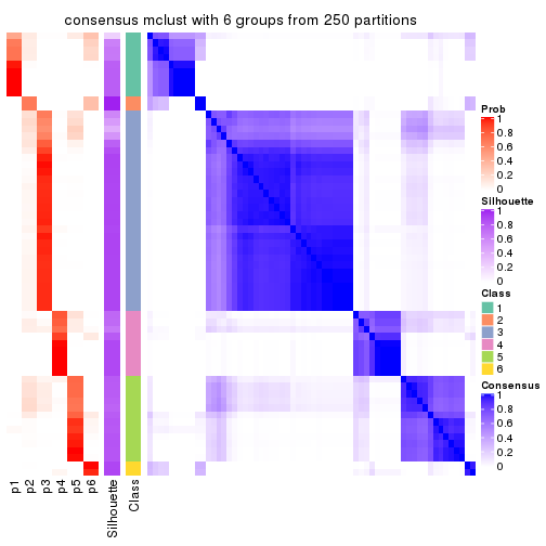
Heatmaps for the membership of samples in all partitions to see how consistent they are:
membership_heatmap(res, k = 2)
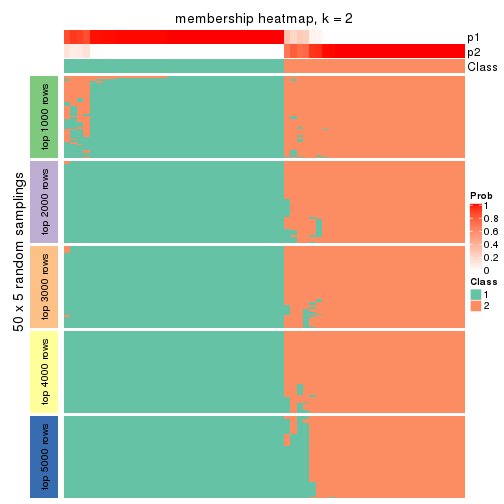
membership_heatmap(res, k = 3)
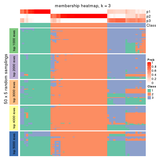
membership_heatmap(res, k = 4)
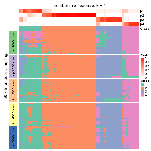
membership_heatmap(res, k = 5)
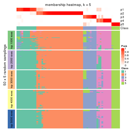
membership_heatmap(res, k = 6)
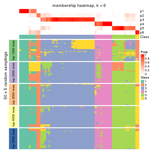
As soon as we have had the classes for columns, we can look for signatures which are significantly different between classes which can be candidate marks for certain classes. Following are the heatmaps for signatures.
Signature heatmaps where rows are scaled:
get_signatures(res, k = 2)
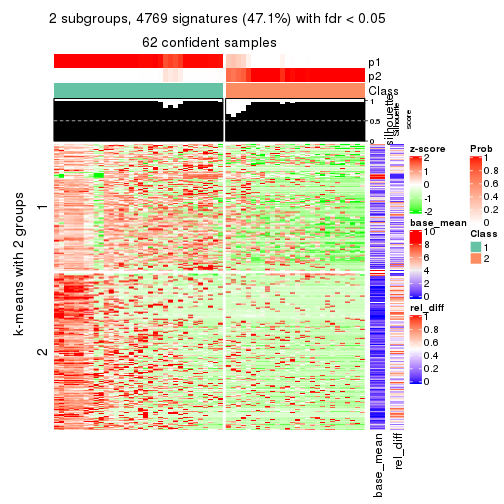
get_signatures(res, k = 3)
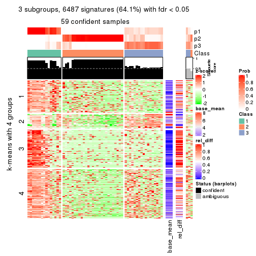
get_signatures(res, k = 4)
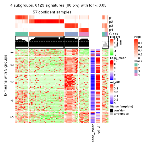
get_signatures(res, k = 5)
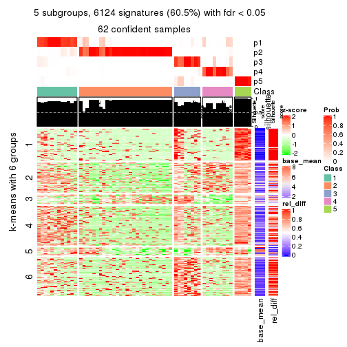
get_signatures(res, k = 6)
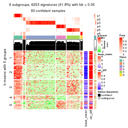
Signature heatmaps where rows are not scaled:
get_signatures(res, k = 2, scale_rows = FALSE)
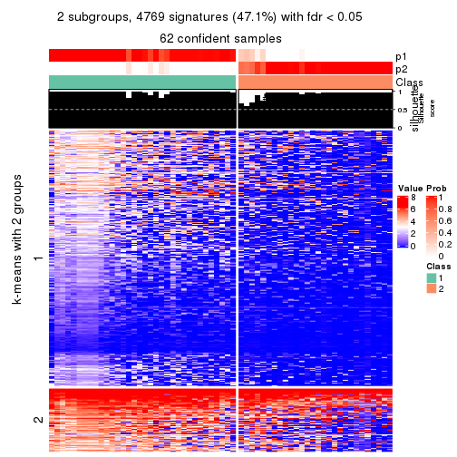
get_signatures(res, k = 3, scale_rows = FALSE)
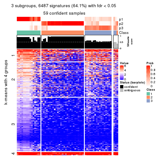
get_signatures(res, k = 4, scale_rows = FALSE)
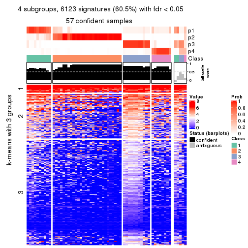
get_signatures(res, k = 5, scale_rows = FALSE)
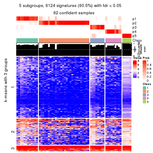
get_signatures(res, k = 6, scale_rows = FALSE)
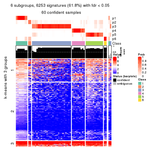
Compare the overlap of signatures from different k:
compare_signatures(res)
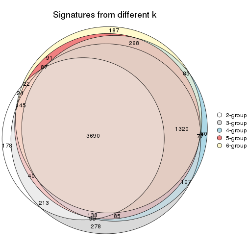
get_signature() returns a data frame invisibly. TO get the list of signatures, the function
call should be assigned to a variable explicitly. In following code, if plot argument is set
to FALSE, no heatmap is plotted while only the differential analysis is performed.
# code only for demonstration
tb = get_signature(res, k = ..., plot = FALSE)
An example of the output of tb is:
#>   which_row         fdr    mean_1    mean_2 scaled_mean_1 scaled_mean_2 km
#> 1        38 0.042760348  8.373488  9.131774    -0.5533452     0.5164555  1
#> 2        40 0.018707592  7.106213  8.469186    -0.6173731     0.5762149  1
#> 3        55 0.019134737 10.221463 11.207825    -0.6159697     0.5749050  1
#> 4        59 0.006059896  5.921854  7.869574    -0.6899429     0.6439467  1
#> 5        60 0.018055526  8.928898 10.211722    -0.6204761     0.5791110  1
#> 6        98 0.009384629 15.714769 14.887706     0.6635654    -0.6193277  2
...
The columns in tb are:
which_row: row indices corresponding to the input matrix.fdr: FDR for the differential test. mean_x: The mean value in group x.scaled_mean_x: The mean value in group x after rows are scaled.km: Row groups if k-means clustering is applied to rows.UMAP plot which shows how samples are separated.
dimension_reduction(res, k = 2, method = "UMAP")
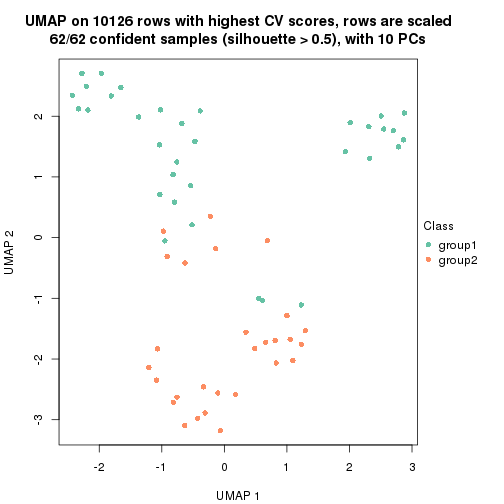
dimension_reduction(res, k = 3, method = "UMAP")
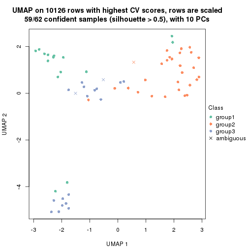
dimension_reduction(res, k = 4, method = "UMAP")
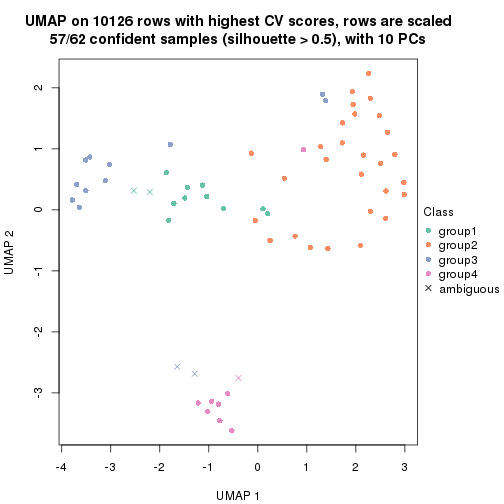
dimension_reduction(res, k = 5, method = "UMAP")
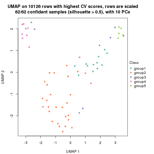
dimension_reduction(res, k = 6, method = "UMAP")
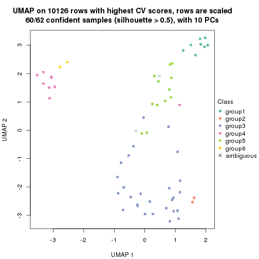
Following heatmap shows how subgroups are split when increasing k:
collect_classes(res)
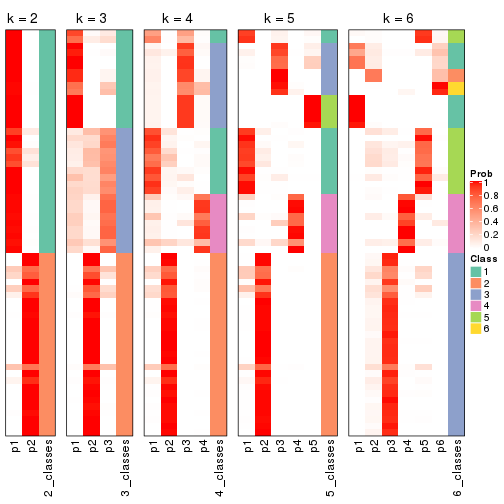
If matrix rows can be associated to genes, consider to use functional_enrichment(res,
...) to perform function enrichment for the signature genes. See this vignette for more detailed explanations.
The object with results only for a single top-value method and a single partition method can be extracted as:
res = res_list["CV", "NMF"]
# you can also extract it by
# res = res_list["CV:NMF"]
A summary of res and all the functions that can be applied to it:
res
#> A 'ConsensusPartition' object with k = 2, 3, 4, 5, 6.
#>   On a matrix with 10126 rows and 62 columns.
#>   Top rows (1000, 2000, 3000, 4000, 5000) are extracted by 'CV' method.
#>   Subgroups are detected by 'NMF' method.
#>   Performed in total 1250 partitions by row resampling.
#>   Best k for subgroups seems to be 2.
#>
#> Following methods can be applied to this 'ConsensusPartition' object:
#>  [1] "cola_report"             "collect_classes"         "collect_plots"
#>  [4] "collect_stats"           "colnames"                "compare_signatures"
#>  [7] "consensus_heatmap"       "dimension_reduction"     "functional_enrichment"
#> [10] "get_anno_col"            "get_anno"                "get_classes"
#> [13] "get_consensus"           "get_matrix"              "get_membership"
#> [16] "get_param"               "get_signatures"          "get_stats"
#> [19] "is_best_k"               "is_stable_k"             "membership_heatmap"
#> [22] "ncol"                    "nrow"                    "plot_ecdf"
#> [25] "rownames"                "select_partition_number" "show"
#> [28] "suggest_best_k"          "test_to_known_factors"
collect_plots() function collects all the plots made from res for all k (number of partitions)
into one single page to provide an easy and fast comparison between different k.
collect_plots(res)
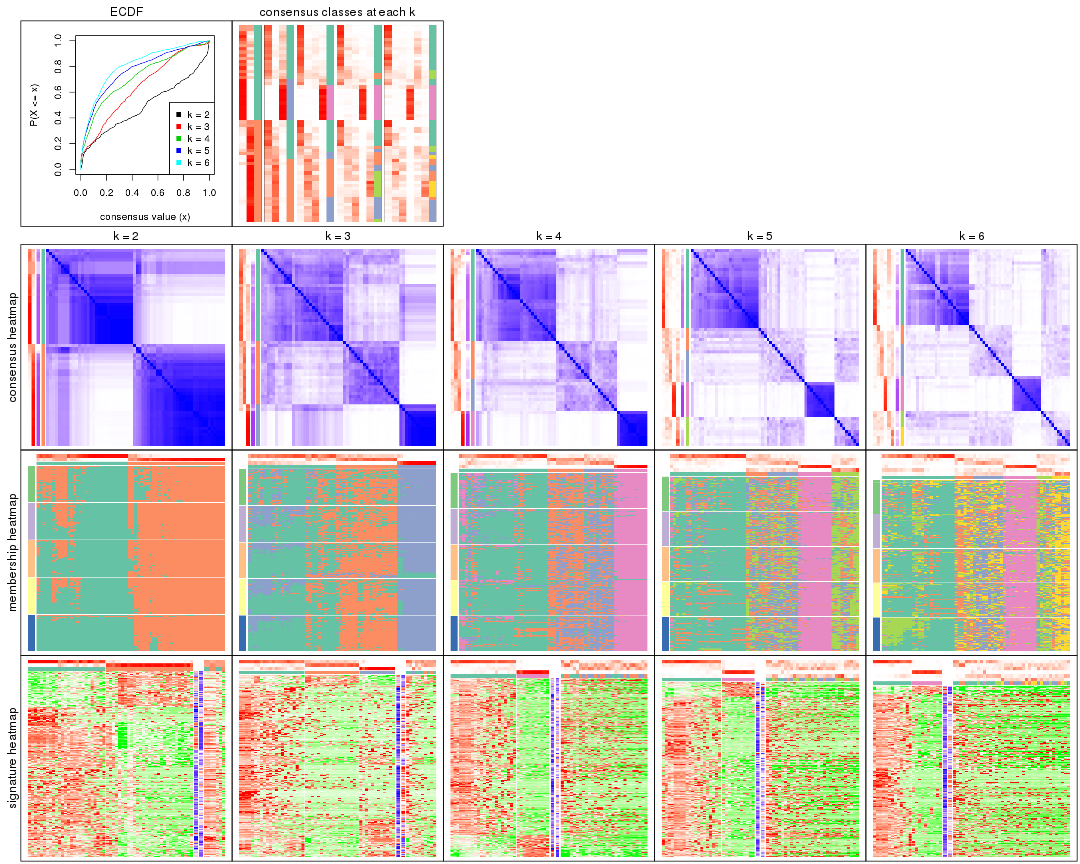
The plots are:
k and the heatmap of
predicted classes for each k.k.k.k.All the plots in panels can be made by individual functions and they are plotted later in this section.
select_partition_number() produces several plots showing different
statistics for choosing “optimized” k. There are following statistics:
k;k, the area increased is defined as \(A_k - A_{k-1}\).The detailed explanations of these statistics can be found in the cola vignette.
Generally speaking, lower PAC score, higher mean silhouette score or higher
concordance corresponds to better partition. Rand index and Jaccard index
measure how similar the current partition is compared to partition with k-1.
If they are too similar, we won't accept k is better than k-1.
select_partition_number(res)
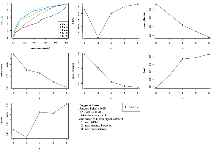
The numeric values for all these statistics can be obtained by get_stats().
get_stats(res)
#>   k 1-PAC mean_silhouette concordance area_increased  Rand Jaccard
#> 2 2 0.479           0.757       0.887         0.4943 0.492   0.492
#> 3 3 0.267           0.642       0.755         0.3093 0.648   0.414
#> 4 4 0.452           0.519       0.727         0.1209 0.872   0.675
#> 5 5 0.503           0.447       0.653         0.0668 0.889   0.662
#> 6 6 0.522           0.380       0.607         0.0474 0.936   0.757
suggest_best_k() suggests the best \(k\) based on these statistics. The rules are as follows:
suggest_best_k(res)
#> [1] 2
Following shows the table of the partitions (You need to click the show/hide
code output link to see it). The membership matrix (columns with name p*)
is inferred by
clue::cl_consensus()
function with the SE method. Basically the value in the membership matrix
represents the probability to belong to a certain group. The finall class
label for an item is determined with the group with highest probability it
belongs to.
In get_classes() function, the entropy is calculated from the membership
matrix and the silhouette score is calculated from the consensus matrix.
cbind(get_classes(res, k = 2), get_membership(res, k = 2))
#>            class entropy silhouette    p1    p2
#> SRR764776      2  0.9686     0.1711 0.396 0.604
#> SRR764777      2  0.9922    -0.0428 0.448 0.552
#> SRR764778      1  0.9988     0.2609 0.520 0.480
#> SRR764779      1  0.9983     0.2731 0.524 0.476
#> SRR764780      1  0.6048     0.7928 0.852 0.148
#> SRR764781      1  0.1843     0.8360 0.972 0.028
#> SRR764782      1  0.6148     0.7855 0.848 0.152
#> SRR764783      1  0.9000     0.6193 0.684 0.316
#> SRR764784      1  0.0672     0.8376 0.992 0.008
#> SRR764785      2  0.3584     0.8774 0.068 0.932
#> SRR764786      1  0.4022     0.8220 0.920 0.080
#> SRR764787      2  0.8144     0.6579 0.252 0.748
#> SRR764788      1  0.9993     0.2512 0.516 0.484
#> SRR764789      1  0.8327     0.6827 0.736 0.264
#> SRR764790      1  0.5178     0.8042 0.884 0.116
#> SRR764791      2  0.6148     0.7877 0.152 0.848
#> SRR764792      2  0.4939     0.8428 0.108 0.892
#> SRR764793      1  0.9491     0.5020 0.632 0.368
#> SRR764794      1  0.8443     0.6483 0.728 0.272
#> SRR764795      1  0.0376     0.8376 0.996 0.004
#> SRR764796      1  0.0376     0.8376 0.996 0.004
#> SRR764797      1  0.6801     0.7700 0.820 0.180
#> SRR764798      2  0.0376     0.8977 0.004 0.996
#> SRR764799      2  0.4431     0.8407 0.092 0.908
#> SRR764800      1  0.9988     0.2589 0.520 0.480
#> SRR764801      2  0.0376     0.8977 0.004 0.996
#> SRR764802      1  0.4939     0.8117 0.892 0.108
#> SRR764803      1  0.7674     0.7353 0.776 0.224
#> SRR764804      2  0.0938     0.8989 0.012 0.988
#> SRR764805      2  0.0672     0.8988 0.008 0.992
#> SRR764806      2  0.0376     0.8991 0.004 0.996
#> SRR764807      2  0.9998    -0.0149 0.492 0.508
#> SRR764808      2  0.7528     0.7096 0.216 0.784
#> SRR764809      2  0.0938     0.8989 0.012 0.988
#> SRR764810      2  0.0672     0.8993 0.008 0.992
#> SRR764811      2  0.4161     0.8628 0.084 0.916
#> SRR764812      2  0.0672     0.8994 0.008 0.992
#> SRR764813      2  0.2423     0.8878 0.040 0.960
#> SRR764814      2  0.0938     0.8968 0.012 0.988
#> SRR764815      1  0.2603     0.8336 0.956 0.044
#> SRR764816      2  0.1414     0.8949 0.020 0.980
#> SRR764817      2  0.4161     0.8489 0.084 0.916
#> SRR1066622     1  0.0672     0.8379 0.992 0.008
#> SRR1066623     1  0.0672     0.8379 0.992 0.008
#> SRR1066624     1  0.0376     0.8369 0.996 0.004
#> SRR1066625     1  0.0672     0.8379 0.992 0.008
#> SRR1066626     1  0.0376     0.8376 0.996 0.004
#> SRR1066627     1  0.0672     0.8379 0.992 0.008
#> SRR1066628     1  0.0672     0.8379 0.992 0.008
#> SRR1066629     1  0.0672     0.8379 0.992 0.008
#> SRR1066630     1  0.0672     0.8379 0.992 0.008
#> SRR1066631     1  0.0672     0.8379 0.992 0.008
#> SRR1066632     2  0.1184     0.8981 0.016 0.984
#> SRR1066633     2  0.0376     0.8990 0.004 0.996
#> SRR1066634     2  0.2603     0.8889 0.044 0.956
#> SRR1066635     2  0.2778     0.8871 0.048 0.952
#> SRR1066636     2  0.0672     0.8989 0.008 0.992
#> SRR1066637     2  0.1414     0.8970 0.020 0.980
#> SRR1066638     2  0.0376     0.8991 0.004 0.996
#> SRR1066639     2  0.0672     0.8989 0.008 0.992
#> SRR1066640     2  0.0672     0.8989 0.008 0.992
#> SRR1066641     2  0.0376     0.8991 0.004 0.996
cbind(get_classes(res, k = 3), get_membership(res, k = 3))
#>            class entropy silhouette    p1    p2    p3
#> SRR764776      1  0.4324     0.6759 0.860 0.028 0.112
#> SRR764777      1  0.4551     0.6848 0.844 0.024 0.132
#> SRR764778      1  0.4723     0.6941 0.824 0.016 0.160
#> SRR764779      1  0.4782     0.6945 0.820 0.016 0.164
#> SRR764780      1  0.5754     0.6546 0.700 0.004 0.296
#> SRR764781      1  0.6168     0.5151 0.588 0.000 0.412
#> SRR764782      1  0.6908     0.6385 0.656 0.036 0.308
#> SRR764783      1  0.5817     0.6932 0.744 0.020 0.236
#> SRR764784      3  0.4733     0.6446 0.196 0.004 0.800
#> SRR764785      1  0.6849     0.0435 0.600 0.380 0.020
#> SRR764786      1  0.7970     0.6110 0.612 0.088 0.300
#> SRR764787      1  0.8693     0.0504 0.496 0.396 0.108
#> SRR764788      1  0.6062     0.6929 0.776 0.064 0.160
#> SRR764789      1  0.9125     0.3705 0.464 0.144 0.392
#> SRR764790      1  0.6699     0.6707 0.700 0.044 0.256
#> SRR764791      1  0.6106     0.5411 0.756 0.200 0.044
#> SRR764792      1  0.4206     0.6046 0.872 0.088 0.040
#> SRR764793      1  0.6793     0.6608 0.740 0.100 0.160
#> SRR764794      1  0.7381     0.6210 0.704 0.132 0.164
#> SRR764795      3  0.5815     0.3970 0.304 0.004 0.692
#> SRR764796      3  0.1289     0.9092 0.032 0.000 0.968
#> SRR764797      1  0.7642     0.6892 0.660 0.092 0.248
#> SRR764798      2  0.6111     0.6008 0.396 0.604 0.000
#> SRR764799      1  0.4978     0.4560 0.780 0.216 0.004
#> SRR764800      1  0.5728     0.6982 0.772 0.032 0.196
#> SRR764801      2  0.5988     0.6592 0.368 0.632 0.000
#> SRR764802      1  0.6661     0.5279 0.588 0.012 0.400
#> SRR764803      1  0.6696     0.6072 0.632 0.020 0.348
#> SRR764804      2  0.4172     0.7477 0.156 0.840 0.004
#> SRR764805      2  0.5365     0.7583 0.252 0.744 0.004
#> SRR764806      2  0.4555     0.7554 0.200 0.800 0.000
#> SRR764807      1  0.8362     0.1078 0.528 0.384 0.088
#> SRR764808      2  0.8209     0.1832 0.456 0.472 0.072
#> SRR764809      2  0.5325     0.7494 0.248 0.748 0.004
#> SRR764810      2  0.4353     0.7638 0.156 0.836 0.008
#> SRR764811      2  0.7013     0.6871 0.324 0.640 0.036
#> SRR764812      2  0.5058     0.7451 0.244 0.756 0.000
#> SRR764813      1  0.7181    -0.2849 0.508 0.468 0.024
#> SRR764814      1  0.5982     0.2449 0.668 0.328 0.004
#> SRR764815      1  0.7513     0.5921 0.604 0.052 0.344
#> SRR764816      1  0.4178     0.5030 0.828 0.172 0.000
#> SRR764817      1  0.3715     0.5525 0.868 0.128 0.004
#> SRR1066622     3  0.0000     0.9340 0.000 0.000 1.000
#> SRR1066623     3  0.0237     0.9319 0.004 0.000 0.996
#> SRR1066624     3  0.0237     0.9322 0.004 0.000 0.996
#> SRR1066625     3  0.0000     0.9340 0.000 0.000 1.000
#> SRR1066626     3  0.0829     0.9251 0.012 0.004 0.984
#> SRR1066627     3  0.0000     0.9340 0.000 0.000 1.000
#> SRR1066628     3  0.0000     0.9340 0.000 0.000 1.000
#> SRR1066629     3  0.0000     0.9340 0.000 0.000 1.000
#> SRR1066630     3  0.0237     0.9313 0.004 0.000 0.996
#> SRR1066631     3  0.0000     0.9340 0.000 0.000 1.000
#> SRR1066632     2  0.5656     0.7428 0.264 0.728 0.008
#> SRR1066633     2  0.4931     0.7514 0.232 0.768 0.000
#> SRR1066634     2  0.6264     0.6114 0.380 0.616 0.004
#> SRR1066635     2  0.7558     0.4848 0.400 0.556 0.044
#> SRR1066636     2  0.4605     0.7513 0.204 0.796 0.000
#> SRR1066637     2  0.5659     0.7525 0.248 0.740 0.012
#> SRR1066638     2  0.5201     0.7633 0.236 0.760 0.004
#> SRR1066639     2  0.5497     0.7199 0.292 0.708 0.000
#> SRR1066640     2  0.4931     0.7511 0.212 0.784 0.004
#> SRR1066641     2  0.5115     0.7633 0.228 0.768 0.004
cbind(get_classes(res, k = 4), get_membership(res, k = 4))
#>            class entropy silhouette    p1    p2    p3    p4
#> SRR764776      1  0.2234    0.74379 0.924 0.064 0.008 0.004
#> SRR764777      1  0.2125    0.74521 0.932 0.052 0.012 0.004
#> SRR764778      1  0.1863    0.74671 0.944 0.040 0.012 0.004
#> SRR764779      1  0.1953    0.74638 0.940 0.044 0.012 0.004
#> SRR764780      1  0.2686    0.75096 0.916 0.012 0.040 0.032
#> SRR764781      1  0.2984    0.74576 0.888 0.000 0.028 0.084
#> SRR764782      1  0.4687    0.73333 0.808 0.028 0.132 0.032
#> SRR764783      1  0.3833    0.74248 0.864 0.024 0.076 0.036
#> SRR764784      1  0.7118    0.30712 0.488 0.024 0.068 0.420
#> SRR764785      1  0.8106   -0.10813 0.392 0.336 0.264 0.008
#> SRR764786      1  0.8616    0.40760 0.516 0.164 0.228 0.092
#> SRR764787      1  0.7576    0.00421 0.440 0.084 0.440 0.036
#> SRR764788      1  0.3979    0.74463 0.844 0.056 0.096 0.004
#> SRR764789      1  0.9338    0.24593 0.444 0.160 0.188 0.208
#> SRR764790      1  0.6322    0.70052 0.728 0.084 0.120 0.068
#> SRR764791      1  0.4426    0.72398 0.796 0.032 0.168 0.004
#> SRR764792      1  0.3711    0.73548 0.836 0.024 0.140 0.000
#> SRR764793      1  0.4341    0.72617 0.820 0.024 0.136 0.020
#> SRR764794      1  0.6451    0.67903 0.712 0.136 0.104 0.048
#> SRR764795      1  0.6346    0.58901 0.668 0.020 0.072 0.240
#> SRR764796      4  0.4419    0.80292 0.088 0.012 0.072 0.828
#> SRR764797      1  0.4175    0.74958 0.844 0.084 0.056 0.016
#> SRR764798      2  0.5722    0.26276 0.148 0.716 0.136 0.000
#> SRR764799      1  0.5666    0.47581 0.616 0.348 0.036 0.000
#> SRR764800      1  0.2911    0.74497 0.900 0.072 0.016 0.012
#> SRR764801      2  0.4662    0.33496 0.112 0.796 0.092 0.000
#> SRR764802      1  0.3876    0.74215 0.856 0.008 0.068 0.068
#> SRR764803      1  0.4185    0.74687 0.844 0.016 0.060 0.080
#> SRR764804      2  0.4853    0.35689 0.036 0.744 0.220 0.000
#> SRR764805      2  0.6455    0.21351 0.060 0.524 0.412 0.004
#> SRR764806      3  0.6097    0.05659 0.056 0.364 0.580 0.000
#> SRR764807      3  0.8668    0.15350 0.360 0.212 0.384 0.044
#> SRR764808      2  0.7955    0.10524 0.160 0.532 0.272 0.036
#> SRR764809      2  0.6196    0.34630 0.100 0.668 0.228 0.004
#> SRR764810      2  0.6361    0.13322 0.044 0.504 0.444 0.008
#> SRR764811      3  0.6903    0.22177 0.108 0.220 0.644 0.028
#> SRR764812      2  0.6139    0.32939 0.100 0.656 0.244 0.000
#> SRR764813      3  0.8199   -0.03347 0.224 0.376 0.384 0.016
#> SRR764814      1  0.6722    0.45696 0.604 0.288 0.100 0.008
#> SRR764815      1  0.6090    0.70242 0.732 0.040 0.144 0.084
#> SRR764816      1  0.4095    0.68130 0.792 0.192 0.016 0.000
#> SRR764817      1  0.3280    0.72407 0.860 0.124 0.016 0.000
#> SRR1066622     4  0.0000    0.97076 0.000 0.000 0.000 1.000
#> SRR1066623     4  0.0000    0.97076 0.000 0.000 0.000 1.000
#> SRR1066624     4  0.1256    0.95314 0.028 0.008 0.000 0.964
#> SRR1066625     4  0.0336    0.96908 0.000 0.000 0.008 0.992
#> SRR1066626     4  0.0992    0.96328 0.008 0.004 0.012 0.976
#> SRR1066627     4  0.0336    0.97091 0.008 0.000 0.000 0.992
#> SRR1066628     4  0.0524    0.97042 0.008 0.000 0.004 0.988
#> SRR1066629     4  0.0000    0.97076 0.000 0.000 0.000 1.000
#> SRR1066630     4  0.0712    0.96843 0.008 0.004 0.004 0.984
#> SRR1066631     4  0.0336    0.97091 0.008 0.000 0.000 0.992
#> SRR1066632     2  0.7184    0.18484 0.144 0.492 0.364 0.000
#> SRR1066633     2  0.6211   -0.05417 0.052 0.488 0.460 0.000
#> SRR1066634     3  0.5613    0.31817 0.156 0.120 0.724 0.000
#> SRR1066635     3  0.8226    0.11537 0.168 0.328 0.468 0.036
#> SRR1066636     3  0.6101    0.11487 0.052 0.388 0.560 0.000
#> SRR1066637     2  0.7125    0.24473 0.116 0.540 0.336 0.008
#> SRR1066638     2  0.6658    0.01560 0.084 0.472 0.444 0.000
#> SRR1066639     3  0.6499    0.23879 0.112 0.276 0.612 0.000
#> SRR1066640     3  0.5662    0.25412 0.072 0.236 0.692 0.000
#> SRR1066641     3  0.6295    0.07482 0.072 0.348 0.580 0.000
cbind(get_classes(res, k = 5), get_membership(res, k = 5))
#>            class entropy silhouette    p1    p2    p3    p4    p5
#> SRR764776      1  0.1928    0.72037 0.920 0.072 0.004 0.000 0.004
#> SRR764777      1  0.1502    0.72236 0.940 0.056 0.004 0.000 0.000
#> SRR764778      1  0.1502    0.72309 0.940 0.056 0.004 0.000 0.000
#> SRR764779      1  0.1731    0.72235 0.932 0.060 0.004 0.000 0.004
#> SRR764780      1  0.0932    0.72344 0.972 0.020 0.004 0.004 0.000
#> SRR764781      1  0.1980    0.72519 0.936 0.020 0.020 0.020 0.004
#> SRR764782      1  0.4778    0.65795 0.776 0.120 0.064 0.004 0.036
#> SRR764783      1  0.3027    0.70462 0.880 0.072 0.032 0.004 0.012
#> SRR764784      1  0.7452    0.21074 0.524 0.124 0.068 0.268 0.016
#> SRR764785      2  0.8660    0.18595 0.224 0.388 0.196 0.016 0.176
#> SRR764786      2  0.8110    0.17545 0.380 0.388 0.128 0.056 0.048
#> SRR764787      3  0.8621   -0.19285 0.300 0.272 0.316 0.028 0.084
#> SRR764788      1  0.4612    0.66127 0.784 0.112 0.060 0.000 0.044
#> SRR764789      2  0.9000    0.23353 0.312 0.356 0.156 0.092 0.084
#> SRR764790      1  0.7110    0.32980 0.552 0.284 0.092 0.036 0.036
#> SRR764791      1  0.6022    0.51906 0.636 0.192 0.152 0.000 0.020
#> SRR764792      1  0.6062    0.52845 0.664 0.148 0.140 0.000 0.048
#> SRR764793      1  0.5719    0.60887 0.712 0.076 0.148 0.008 0.056
#> SRR764794      1  0.7265    0.13184 0.492 0.348 0.080 0.024 0.056
#> SRR764795      1  0.5786    0.57746 0.724 0.100 0.064 0.096 0.016
#> SRR764796      4  0.6723    0.56876 0.080 0.092 0.156 0.648 0.024
#> SRR764797      1  0.4010    0.69577 0.820 0.112 0.012 0.008 0.048
#> SRR764798      2  0.7546   -0.23765 0.088 0.400 0.112 0.004 0.396
#> SRR764799      1  0.6449    0.37620 0.588 0.244 0.032 0.000 0.136
#> SRR764800      1  0.2116    0.72038 0.912 0.076 0.004 0.000 0.008
#> SRR764801      5  0.7068    0.14494 0.076 0.360 0.092 0.000 0.472
#> SRR764802      1  0.3822    0.70040 0.844 0.044 0.076 0.028 0.008
#> SRR764803      1  0.2735    0.72304 0.900 0.044 0.036 0.016 0.004
#> SRR764804      5  0.2522    0.37474 0.012 0.056 0.028 0.000 0.904
#> SRR764805      5  0.7522    0.09300 0.040 0.316 0.260 0.000 0.384
#> SRR764806      5  0.6973   -0.03898 0.020 0.184 0.380 0.000 0.416
#> SRR764807      2  0.8917   -0.02067 0.220 0.284 0.280 0.016 0.200
#> SRR764808      2  0.8138    0.00114 0.088 0.440 0.192 0.016 0.264
#> SRR764809      5  0.6542    0.31987 0.052 0.184 0.136 0.004 0.624
#> SRR764810      3  0.7147   -0.02654 0.012 0.204 0.400 0.008 0.376
#> SRR764811      3  0.7987    0.18748 0.072 0.252 0.476 0.024 0.176
#> SRR764812      5  0.5035    0.36490 0.096 0.084 0.060 0.000 0.760
#> SRR764813      2  0.8752   -0.05120 0.160 0.312 0.252 0.012 0.264
#> SRR764814      1  0.7086    0.32721 0.576 0.184 0.076 0.004 0.160
#> SRR764815      1  0.6477    0.51447 0.636 0.204 0.104 0.040 0.016
#> SRR764816      1  0.4398    0.65116 0.780 0.144 0.016 0.000 0.060
#> SRR764817      1  0.3207    0.70434 0.864 0.084 0.012 0.000 0.040
#> SRR1066622     4  0.1016    0.93083 0.008 0.004 0.012 0.972 0.004
#> SRR1066623     4  0.1659    0.92742 0.016 0.024 0.008 0.948 0.004
#> SRR1066624     4  0.1617    0.92075 0.020 0.020 0.012 0.948 0.000
#> SRR1066625     4  0.1277    0.93007 0.004 0.028 0.004 0.960 0.004
#> SRR1066626     4  0.2246    0.91281 0.020 0.048 0.008 0.920 0.004
#> SRR1066627     4  0.1280    0.93067 0.008 0.008 0.024 0.960 0.000
#> SRR1066628     4  0.0771    0.93042 0.000 0.020 0.004 0.976 0.000
#> SRR1066629     4  0.0902    0.93059 0.008 0.008 0.004 0.976 0.004
#> SRR1066630     4  0.2388    0.90302 0.000 0.072 0.028 0.900 0.000
#> SRR1066631     4  0.1622    0.92932 0.004 0.028 0.016 0.948 0.004
#> SRR1066632     5  0.6520    0.27468 0.116 0.096 0.136 0.004 0.648
#> SRR1066633     3  0.8193    0.15563 0.084 0.276 0.376 0.008 0.256
#> SRR1066634     3  0.6138    0.24832 0.104 0.060 0.680 0.008 0.148
#> SRR1066635     3  0.7983    0.18375 0.064 0.264 0.464 0.024 0.184
#> SRR1066636     3  0.7289    0.21317 0.044 0.192 0.500 0.004 0.260
#> SRR1066637     5  0.7131    0.26319 0.096 0.124 0.160 0.016 0.604
#> SRR1066638     5  0.7866    0.00451 0.052 0.296 0.312 0.004 0.336
#> SRR1066639     3  0.7485    0.19874 0.100 0.144 0.500 0.000 0.256
#> SRR1066640     3  0.6844    0.19845 0.048 0.092 0.560 0.012 0.288
#> SRR1066641     3  0.7536   -0.00525 0.028 0.240 0.400 0.008 0.324
cbind(get_classes(res, k = 6), get_membership(res, k = 6))
#>            class entropy silhouette    p1    p2    p3    p4    p5    p6
#> SRR764776      1  0.1334    0.61794 0.948 0.032 0.000 0.000 0.020 0.000
#> SRR764777      1  0.1168    0.61921 0.956 0.028 0.000 0.000 0.016 0.000
#> SRR764778      1  0.0909    0.62059 0.968 0.020 0.000 0.000 0.012 0.000
#> SRR764779      1  0.1168    0.61909 0.956 0.028 0.000 0.000 0.016 0.000
#> SRR764780      1  0.2546    0.61508 0.876 0.004 0.008 0.004 0.104 0.004
#> SRR764781      1  0.2099    0.62091 0.904 0.004 0.004 0.008 0.080 0.000
#> SRR764782      1  0.6235    0.40390 0.568 0.024 0.032 0.012 0.296 0.068
#> SRR764783      1  0.4336    0.56611 0.748 0.020 0.024 0.004 0.192 0.012
#> SRR764784      1  0.8032    0.01510 0.388 0.020 0.048 0.184 0.296 0.064
#> SRR764785      5  0.8714    0.14398 0.128 0.220 0.152 0.004 0.340 0.156
#> SRR764786      5  0.8475    0.30201 0.216 0.136 0.140 0.028 0.416 0.064
#> SRR764787      5  0.8470    0.16252 0.176 0.080 0.208 0.004 0.372 0.160
#> SRR764788      1  0.5421    0.49431 0.644 0.032 0.012 0.004 0.256 0.052
#> SRR764789      5  0.8603    0.25712 0.148 0.124 0.160 0.036 0.436 0.096
#> SRR764790      1  0.7606   -0.21179 0.408 0.092 0.068 0.024 0.364 0.044
#> SRR764791      1  0.7279    0.10335 0.448 0.040 0.112 0.004 0.328 0.068
#> SRR764792      1  0.7292    0.04436 0.428 0.048 0.068 0.004 0.356 0.096
#> SRR764793      1  0.6245    0.38539 0.564 0.028 0.044 0.004 0.296 0.064
#> SRR764794      5  0.7647    0.19450 0.360 0.112 0.064 0.012 0.396 0.056
#> SRR764795      1  0.7018    0.36318 0.552 0.040 0.024 0.072 0.248 0.064
#> SRR764796      4  0.7774    0.35383 0.080 0.024 0.100 0.520 0.184 0.092
#> SRR764797      1  0.3875    0.59433 0.816 0.064 0.020 0.000 0.084 0.016
#> SRR764798      2  0.5002    0.25580 0.132 0.728 0.020 0.000 0.028 0.092
#> SRR764799      1  0.4223    0.29348 0.612 0.368 0.004 0.000 0.000 0.016
#> SRR764800      1  0.1863    0.61743 0.924 0.056 0.000 0.004 0.008 0.008
#> SRR764801      2  0.4825    0.22943 0.120 0.736 0.044 0.000 0.004 0.096
#> SRR764802      1  0.5126    0.53399 0.688 0.020 0.036 0.008 0.224 0.024
#> SRR764803      1  0.4406    0.59560 0.780 0.012 0.036 0.024 0.132 0.016
#> SRR764804      6  0.5371    0.36020 0.020 0.264 0.072 0.000 0.012 0.632
#> SRR764805      2  0.8343   -0.07494 0.044 0.332 0.232 0.004 0.160 0.228
#> SRR764806      3  0.7197    0.18914 0.012 0.196 0.480 0.000 0.108 0.204
#> SRR764807      3  0.8855   -0.00207 0.156 0.080 0.296 0.020 0.280 0.168
#> SRR764808      2  0.8914    0.01870 0.084 0.284 0.240 0.016 0.156 0.220
#> SRR764809      6  0.7690    0.17776 0.048 0.316 0.136 0.000 0.100 0.400
#> SRR764810      3  0.8058    0.09373 0.024 0.268 0.332 0.024 0.072 0.280
#> SRR764811      3  0.8190    0.12564 0.052 0.164 0.420 0.008 0.172 0.184
#> SRR764812      6  0.5392    0.42350 0.084 0.180 0.028 0.000 0.024 0.684
#> SRR764813      6  0.9404   -0.09072 0.180 0.160 0.232 0.032 0.160 0.236
#> SRR764814      1  0.6292    0.18864 0.536 0.316 0.072 0.000 0.056 0.020
#> SRR764815      1  0.6492    0.19831 0.528 0.040 0.072 0.012 0.324 0.024
#> SRR764816      1  0.3371    0.54006 0.796 0.180 0.004 0.000 0.008 0.012
#> SRR764817      1  0.2734    0.59123 0.864 0.104 0.000 0.000 0.024 0.008
#> SRR1066622     4  0.1231    0.87771 0.012 0.012 0.000 0.960 0.012 0.004
#> SRR1066623     4  0.2874    0.86804 0.020 0.020 0.020 0.892 0.028 0.020
#> SRR1066624     4  0.2567    0.82110 0.100 0.012 0.000 0.876 0.004 0.008
#> SRR1066625     4  0.1766    0.87728 0.004 0.012 0.008 0.940 0.020 0.016
#> SRR1066626     4  0.3731    0.83549 0.044 0.004 0.012 0.824 0.100 0.016
#> SRR1066627     4  0.2357    0.87734 0.008 0.008 0.024 0.908 0.048 0.004
#> SRR1066628     4  0.1799    0.87930 0.004 0.012 0.004 0.932 0.044 0.004
#> SRR1066629     4  0.1425    0.87796 0.000 0.008 0.008 0.952 0.020 0.012
#> SRR1066630     4  0.4631    0.81767 0.020 0.024 0.044 0.788 0.084 0.040
#> SRR1066631     4  0.2227    0.87376 0.012 0.004 0.012 0.916 0.044 0.012
#> SRR1066632     6  0.5367    0.33461 0.104 0.040 0.068 0.004 0.056 0.728
#> SRR1066633     3  0.8052    0.11903 0.044 0.220 0.376 0.000 0.132 0.228
#> SRR1066634     3  0.7647    0.23155 0.080 0.108 0.496 0.000 0.136 0.180
#> SRR1066635     2  0.8458   -0.02663 0.076 0.348 0.292 0.012 0.156 0.116
#> SRR1066636     3  0.7757    0.21094 0.032 0.216 0.428 0.004 0.100 0.220
#> SRR1066637     6  0.6343    0.31348 0.072 0.088 0.084 0.016 0.072 0.668
#> SRR1066638     2  0.8423   -0.05218 0.068 0.280 0.248 0.000 0.136 0.268
#> SRR1066639     3  0.7374    0.24131 0.072 0.108 0.492 0.004 0.060 0.264
#> SRR1066640     3  0.5957    0.31280 0.020 0.084 0.624 0.000 0.052 0.220
#> SRR1066641     3  0.8116    0.11783 0.044 0.236 0.344 0.000 0.128 0.248
Heatmaps for the consensus matrix. It visualizes the probability of two samples to be in a same group.
consensus_heatmap(res, k = 2)
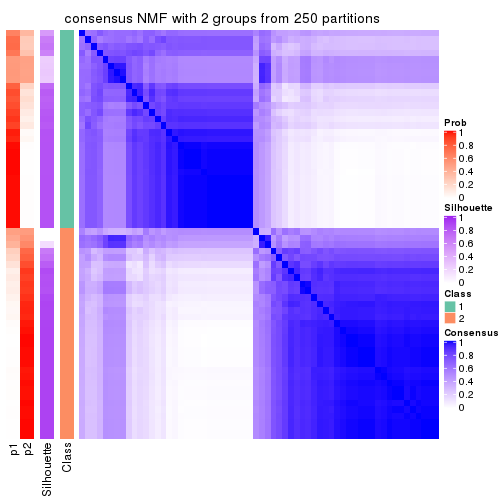
consensus_heatmap(res, k = 3)
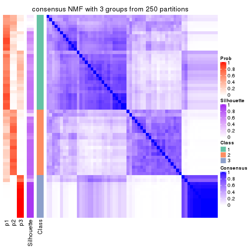
consensus_heatmap(res, k = 4)
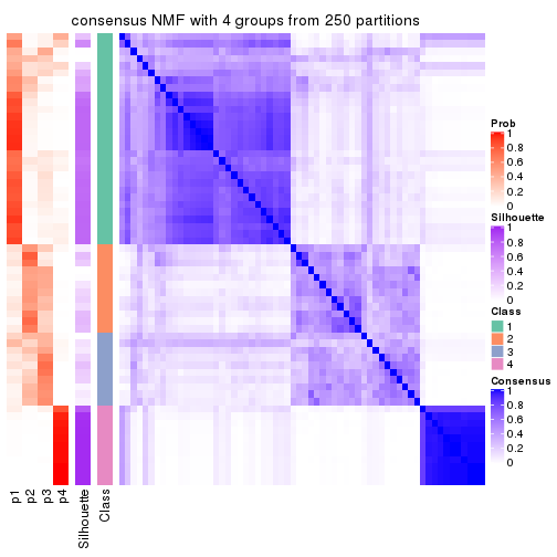
consensus_heatmap(res, k = 5)
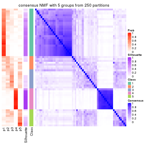
consensus_heatmap(res, k = 6)
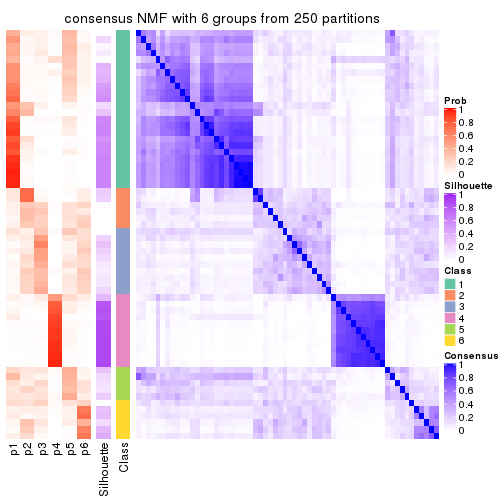
Heatmaps for the membership of samples in all partitions to see how consistent they are:
membership_heatmap(res, k = 2)
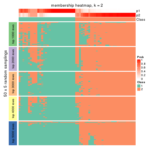
membership_heatmap(res, k = 3)
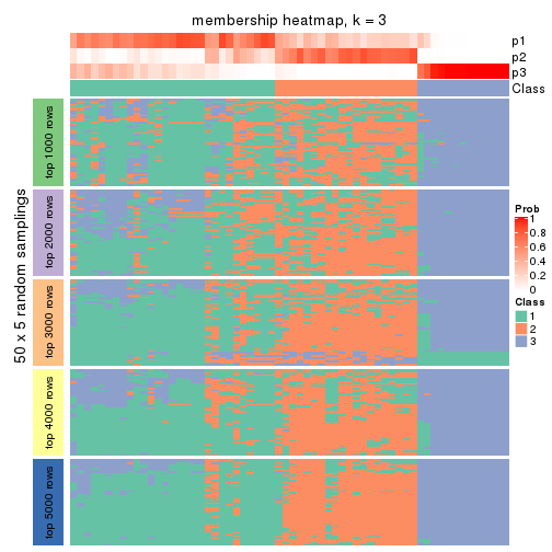
membership_heatmap(res, k = 4)
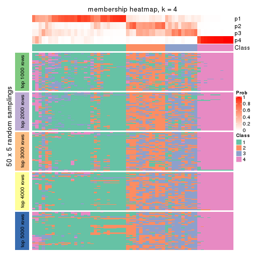
membership_heatmap(res, k = 5)
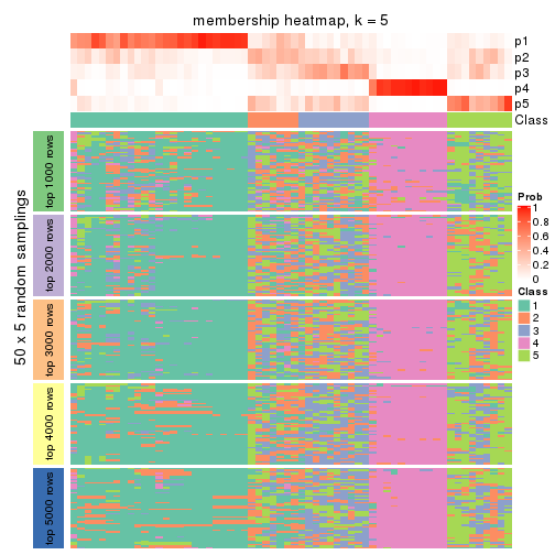
membership_heatmap(res, k = 6)
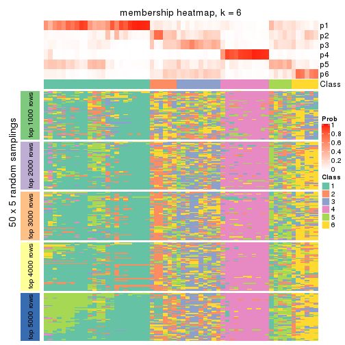
As soon as we have had the classes for columns, we can look for signatures which are significantly different between classes which can be candidate marks for certain classes. Following are the heatmaps for signatures.
Signature heatmaps where rows are scaled:
get_signatures(res, k = 2)
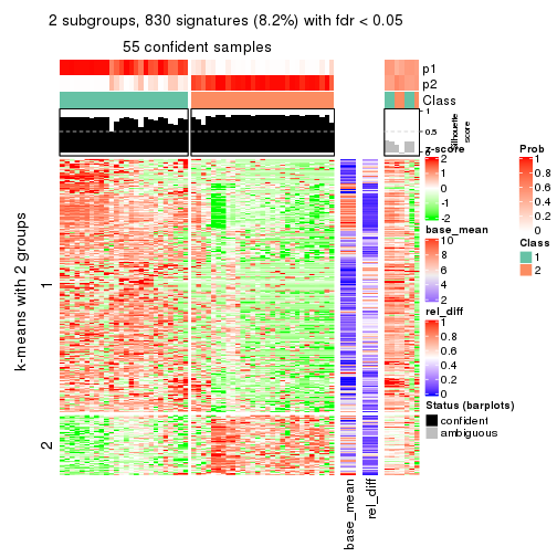
get_signatures(res, k = 3)
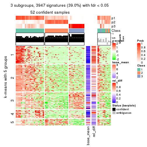
get_signatures(res, k = 4)
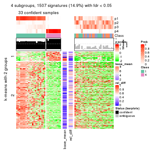
get_signatures(res, k = 5)
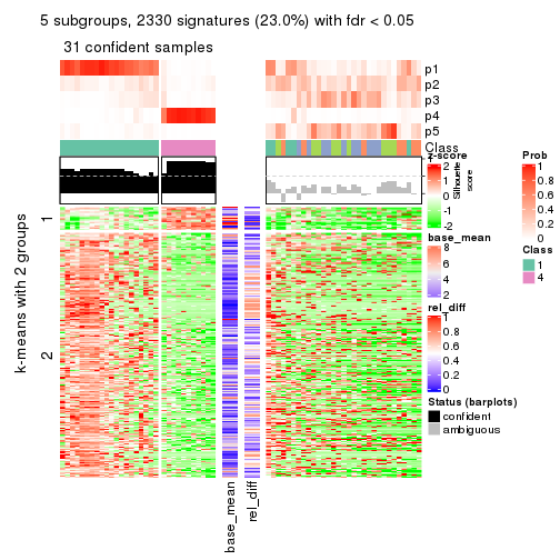
get_signatures(res, k = 6)
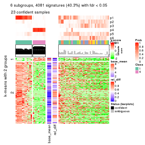
Signature heatmaps where rows are not scaled:
get_signatures(res, k = 2, scale_rows = FALSE)
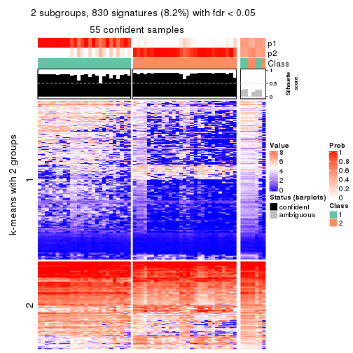
get_signatures(res, k = 3, scale_rows = FALSE)
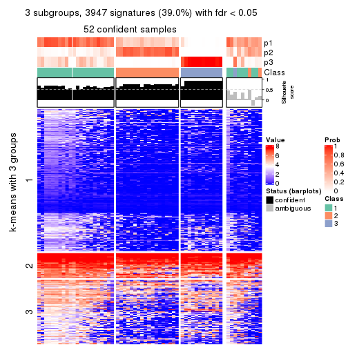
get_signatures(res, k = 4, scale_rows = FALSE)
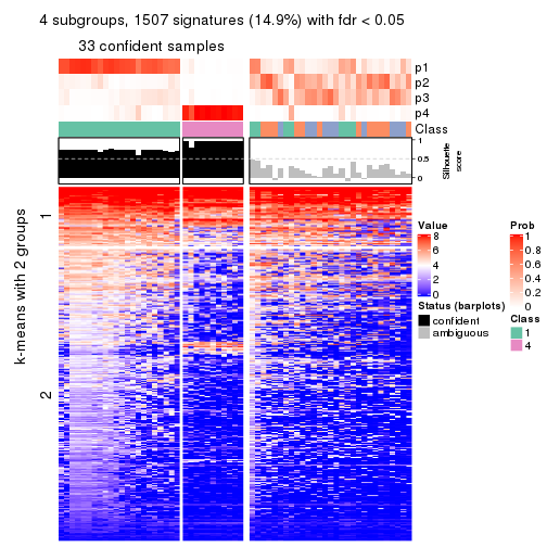
get_signatures(res, k = 5, scale_rows = FALSE)
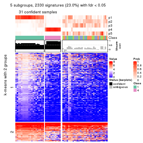
get_signatures(res, k = 6, scale_rows = FALSE)
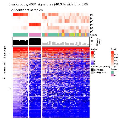
Compare the overlap of signatures from different k:
compare_signatures(res)
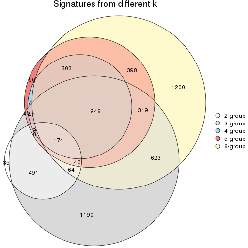
get_signature() returns a data frame invisibly. TO get the list of signatures, the function
call should be assigned to a variable explicitly. In following code, if plot argument is set
to FALSE, no heatmap is plotted while only the differential analysis is performed.
# code only for demonstration
tb = get_signature(res, k = ..., plot = FALSE)
An example of the output of tb is:
#>   which_row         fdr    mean_1    mean_2 scaled_mean_1 scaled_mean_2 km
#> 1        38 0.042760348  8.373488  9.131774    -0.5533452     0.5164555  1
#> 2        40 0.018707592  7.106213  8.469186    -0.6173731     0.5762149  1
#> 3        55 0.019134737 10.221463 11.207825    -0.6159697     0.5749050  1
#> 4        59 0.006059896  5.921854  7.869574    -0.6899429     0.6439467  1
#> 5        60 0.018055526  8.928898 10.211722    -0.6204761     0.5791110  1
#> 6        98 0.009384629 15.714769 14.887706     0.6635654    -0.6193277  2
...
The columns in tb are:
which_row: row indices corresponding to the input matrix.fdr: FDR for the differential test. mean_x: The mean value in group x.scaled_mean_x: The mean value in group x after rows are scaled.km: Row groups if k-means clustering is applied to rows.UMAP plot which shows how samples are separated.
dimension_reduction(res, k = 2, method = "UMAP")
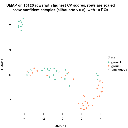
dimension_reduction(res, k = 3, method = "UMAP")
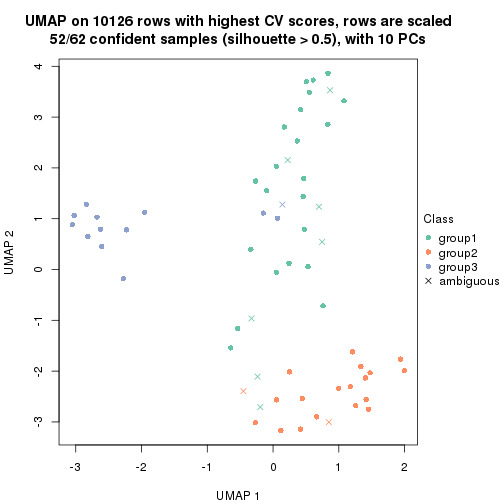
dimension_reduction(res, k = 4, method = "UMAP")
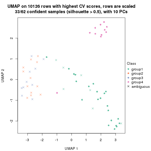
dimension_reduction(res, k = 5, method = "UMAP")
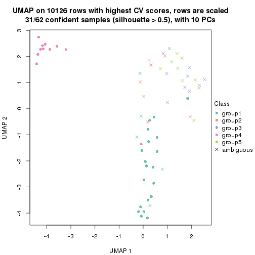
dimension_reduction(res, k = 6, method = "UMAP")
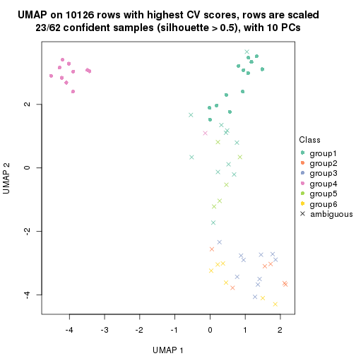
Following heatmap shows how subgroups are split when increasing k:
collect_classes(res)
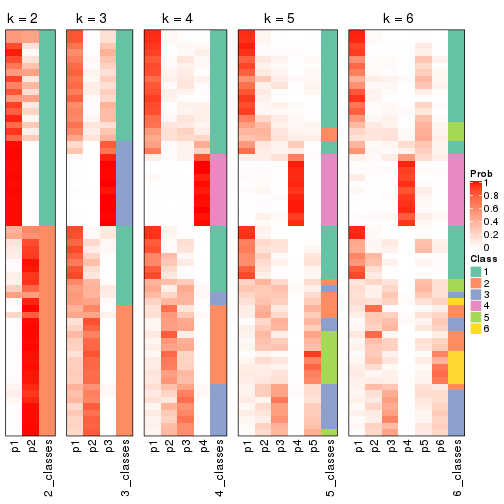
If matrix rows can be associated to genes, consider to use functional_enrichment(res,
...) to perform function enrichment for the signature genes. See this vignette for more detailed explanations.
The object with results only for a single top-value method and a single partition method can be extracted as:
res = res_list["MAD", "hclust"]
# you can also extract it by
# res = res_list["MAD:hclust"]
A summary of res and all the functions that can be applied to it:
res
#> A 'ConsensusPartition' object with k = 2, 3, 4, 5, 6.
#>   On a matrix with 10126 rows and 62 columns.
#>   Top rows (1000, 2000, 3000, 4000, 5000) are extracted by 'MAD' method.
#>   Subgroups are detected by 'hclust' method.
#>   Performed in total 1250 partitions by row resampling.
#>   Best k for subgroups seems to be 2.
#>
#> Following methods can be applied to this 'ConsensusPartition' object:
#>  [1] "cola_report"             "collect_classes"         "collect_plots"
#>  [4] "collect_stats"           "colnames"                "compare_signatures"
#>  [7] "consensus_heatmap"       "dimension_reduction"     "functional_enrichment"
#> [10] "get_anno_col"            "get_anno"                "get_classes"
#> [13] "get_consensus"           "get_matrix"              "get_membership"
#> [16] "get_param"               "get_signatures"          "get_stats"
#> [19] "is_best_k"               "is_stable_k"             "membership_heatmap"
#> [22] "ncol"                    "nrow"                    "plot_ecdf"
#> [25] "rownames"                "select_partition_number" "show"
#> [28] "suggest_best_k"          "test_to_known_factors"
collect_plots() function collects all the plots made from res for all k (number of partitions)
into one single page to provide an easy and fast comparison between different k.
collect_plots(res)
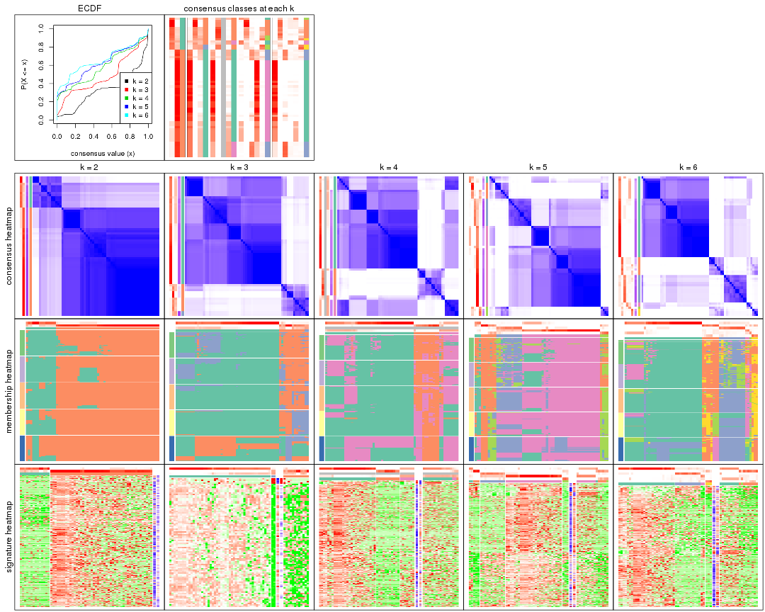
The plots are:
k and the heatmap of
predicted classes for each k.k.k.k.All the plots in panels can be made by individual functions and they are plotted later in this section.
select_partition_number() produces several plots showing different
statistics for choosing “optimized” k. There are following statistics:
k;k, the area increased is defined as \(A_k - A_{k-1}\).The detailed explanations of these statistics can be found in the cola vignette.
Generally speaking, lower PAC score, higher mean silhouette score or higher
concordance corresponds to better partition. Rand index and Jaccard index
measure how similar the current partition is compared to partition with k-1.
If they are too similar, we won't accept k is better than k-1.
select_partition_number(res)
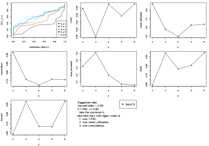
The numeric values for all these statistics can be obtained by get_stats().
get_stats(res)
#>   k 1-PAC mean_silhouette concordance area_increased  Rand Jaccard
#> 2 2 0.458           0.870       0.914         0.3217 0.645   0.645
#> 3 3 0.381           0.580       0.760         0.5087 0.987   0.980
#> 4 4 0.469           0.498       0.727         0.1980 0.820   0.723
#> 5 5 0.437           0.628       0.761         0.0716 0.857   0.718
#> 6 6 0.470           0.636       0.758         0.0592 0.994   0.984
suggest_best_k() suggests the best \(k\) based on these statistics. The rules are as follows:
suggest_best_k(res)
#> [1] 2
Following shows the table of the partitions (You need to click the show/hide
code output link to see it). The membership matrix (columns with name p*)
is inferred by
clue::cl_consensus()
function with the SE method. Basically the value in the membership matrix
represents the probability to belong to a certain group. The finall class
label for an item is determined with the group with highest probability it
belongs to.
In get_classes() function, the entropy is calculated from the membership
matrix and the silhouette score is calculated from the consensus matrix.
cbind(get_classes(res, k = 2), get_membership(res, k = 2))
#>            class entropy silhouette    p1    p2
#> SRR764776      2  0.0000      0.932 0.000 1.000
#> SRR764777      2  0.0000      0.932 0.000 1.000
#> SRR764778      2  0.0000      0.932 0.000 1.000
#> SRR764779      2  0.0000      0.932 0.000 1.000
#> SRR764780      2  0.0000      0.932 0.000 1.000
#> SRR764781      2  0.0000      0.932 0.000 1.000
#> SRR764782      2  0.0000      0.932 0.000 1.000
#> SRR764783      2  0.0000      0.932 0.000 1.000
#> SRR764784      2  0.0000      0.932 0.000 1.000
#> SRR764785      1  0.9815      0.536 0.580 0.420
#> SRR764786      1  0.8327      0.806 0.736 0.264
#> SRR764787      2  0.0938      0.930 0.012 0.988
#> SRR764788      2  0.0000      0.932 0.000 1.000
#> SRR764789      2  0.3114      0.906 0.056 0.944
#> SRR764790      1  0.0000      0.745 1.000 0.000
#> SRR764791      2  0.0672      0.931 0.008 0.992
#> SRR764792      2  0.0376      0.931 0.004 0.996
#> SRR764793      2  0.0000      0.932 0.000 1.000
#> SRR764794      2  0.1414      0.928 0.020 0.980
#> SRR764795      2  0.0000      0.932 0.000 1.000
#> SRR764796      2  0.0000      0.932 0.000 1.000
#> SRR764797      2  0.0000      0.932 0.000 1.000
#> SRR764798      2  0.3114      0.910 0.056 0.944
#> SRR764799      2  0.0000      0.932 0.000 1.000
#> SRR764800      2  0.0000      0.932 0.000 1.000
#> SRR764801      2  0.3114      0.910 0.056 0.944
#> SRR764802      2  0.0000      0.932 0.000 1.000
#> SRR764803      2  0.0000      0.932 0.000 1.000
#> SRR764804      1  0.7883      0.845 0.764 0.236
#> SRR764805      1  0.8813      0.790 0.700 0.300
#> SRR764806      2  0.4690      0.870 0.100 0.900
#> SRR764807      1  0.0000      0.745 1.000 0.000
#> SRR764808      1  0.0000      0.745 1.000 0.000
#> SRR764809      1  0.8909      0.780 0.692 0.308
#> SRR764810      1  0.8909      0.780 0.692 0.308
#> SRR764811      1  0.7453      0.849 0.788 0.212
#> SRR764812      1  0.7815      0.846 0.768 0.232
#> SRR764813      1  0.7602      0.849 0.780 0.220
#> SRR764814      2  0.0000      0.932 0.000 1.000
#> SRR764815      2  0.0938      0.930 0.012 0.988
#> SRR764816      2  0.0000      0.932 0.000 1.000
#> SRR764817      2  0.0000      0.932 0.000 1.000
#> SRR1066622     2  0.6712      0.772 0.176 0.824
#> SRR1066623     2  0.6712      0.772 0.176 0.824
#> SRR1066624     2  0.3879      0.889 0.076 0.924
#> SRR1066625     2  0.6531      0.783 0.168 0.832
#> SRR1066626     2  0.6712      0.772 0.176 0.824
#> SRR1066627     2  0.6712      0.772 0.176 0.824
#> SRR1066628     2  0.6712      0.772 0.176 0.824
#> SRR1066629     2  0.6712      0.772 0.176 0.824
#> SRR1066630     1  0.7139      0.823 0.804 0.196
#> SRR1066631     2  0.6712      0.772 0.176 0.824
#> SRR1066632     2  0.3879      0.899 0.076 0.924
#> SRR1066633     2  0.3431      0.908 0.064 0.936
#> SRR1066634     2  0.2778      0.918 0.048 0.952
#> SRR1066635     2  0.6712      0.764 0.176 0.824
#> SRR1066636     2  0.3431      0.908 0.064 0.936
#> SRR1066637     2  0.3431      0.908 0.064 0.936
#> SRR1066638     2  0.2043      0.923 0.032 0.968
#> SRR1066639     2  0.3584      0.905 0.068 0.932
#> SRR1066640     2  0.3274      0.910 0.060 0.940
#> SRR1066641     1  0.7139      0.845 0.804 0.196
cbind(get_classes(res, k = 3), get_membership(res, k = 3))
#>            class entropy silhouette    p1    p2    p3
#> SRR764776      1  0.0000     0.8250 1.000 0.000 0.000
#> SRR764777      1  0.0000     0.8250 1.000 0.000 0.000
#> SRR764778      1  0.0000     0.8250 1.000 0.000 0.000
#> SRR764779      1  0.0000     0.8250 1.000 0.000 0.000
#> SRR764780      1  0.0000     0.8250 1.000 0.000 0.000
#> SRR764781      1  0.0000     0.8250 1.000 0.000 0.000
#> SRR764782      1  0.0000     0.8250 1.000 0.000 0.000
#> SRR764783      1  0.0000     0.8250 1.000 0.000 0.000
#> SRR764784      1  0.0000     0.8250 1.000 0.000 0.000
#> SRR764785      2  0.9920     0.0981 0.280 0.388 0.332
#> SRR764786      2  0.8902     0.1826 0.144 0.536 0.320
#> SRR764787      1  0.1529     0.8177 0.960 0.000 0.040
#> SRR764788      1  0.0000     0.8250 1.000 0.000 0.000
#> SRR764789      1  0.3030     0.7988 0.904 0.004 0.092
#> SRR764790      2  0.1031     0.2211 0.000 0.976 0.024
#> SRR764791      1  0.0892     0.8243 0.980 0.000 0.020
#> SRR764792      1  0.0892     0.8236 0.980 0.000 0.020
#> SRR764793      1  0.0000     0.8250 1.000 0.000 0.000
#> SRR764794      1  0.2066     0.8028 0.940 0.000 0.060
#> SRR764795      1  0.0000     0.8250 1.000 0.000 0.000
#> SRR764796      1  0.0592     0.8243 0.988 0.000 0.012
#> SRR764797      1  0.3116     0.8064 0.892 0.000 0.108
#> SRR764798      1  0.5733     0.6859 0.676 0.000 0.324
#> SRR764799      1  0.3038     0.8061 0.896 0.000 0.104
#> SRR764800      1  0.3038     0.8061 0.896 0.000 0.104
#> SRR764801      1  0.5733     0.6859 0.676 0.000 0.324
#> SRR764802      1  0.0000     0.8250 1.000 0.000 0.000
#> SRR764803      1  0.0000     0.8250 1.000 0.000 0.000
#> SRR764804      2  0.7824    -0.4453 0.064 0.580 0.356
#> SRR764805      2  0.8334    -0.9160 0.080 0.480 0.440
#> SRR764806      1  0.6935     0.6626 0.652 0.036 0.312
#> SRR764807      2  0.0237     0.2107 0.000 0.996 0.004
#> SRR764808      2  0.0237     0.2153 0.000 0.996 0.004
#> SRR764809      3  0.8342     0.9232 0.080 0.456 0.464
#> SRR764810      3  0.8135     0.9222 0.068 0.448 0.484
#> SRR764811      2  0.7491    -0.4218 0.056 0.620 0.324
#> SRR764812      2  0.7683    -0.3951 0.064 0.608 0.328
#> SRR764813      2  0.7279    -0.2665 0.056 0.652 0.292
#> SRR764814      1  0.3038     0.8061 0.896 0.000 0.104
#> SRR764815      1  0.3879     0.7930 0.848 0.000 0.152
#> SRR764816      1  0.3038     0.8061 0.896 0.000 0.104
#> SRR764817      1  0.3038     0.8061 0.896 0.000 0.104
#> SRR1066622     1  0.6075     0.5746 0.676 0.008 0.316
#> SRR1066623     1  0.6075     0.5746 0.676 0.008 0.316
#> SRR1066624     1  0.4733     0.6953 0.800 0.004 0.196
#> SRR1066625     1  0.5958     0.5908 0.692 0.008 0.300
#> SRR1066626     1  0.6075     0.5746 0.676 0.008 0.316
#> SRR1066627     1  0.6075     0.5746 0.676 0.008 0.316
#> SRR1066628     1  0.6075     0.5746 0.676 0.008 0.316
#> SRR1066629     1  0.6075     0.5746 0.676 0.008 0.316
#> SRR1066630     2  0.7722     0.2108 0.076 0.628 0.296
#> SRR1066631     1  0.6075     0.5746 0.676 0.008 0.316
#> SRR1066632     1  0.6255     0.7010 0.684 0.016 0.300
#> SRR1066633     1  0.5733     0.6923 0.676 0.000 0.324
#> SRR1066634     1  0.5553     0.7264 0.724 0.004 0.272
#> SRR1066635     1  0.8311     0.5966 0.616 0.132 0.252
#> SRR1066636     1  0.5733     0.6923 0.676 0.000 0.324
#> SRR1066637     1  0.5760     0.6904 0.672 0.000 0.328
#> SRR1066638     1  0.5216     0.7396 0.740 0.000 0.260
#> SRR1066639     1  0.6102     0.6897 0.672 0.008 0.320
#> SRR1066640     1  0.5760     0.6877 0.672 0.000 0.328
#> SRR1066641     2  0.6986    -0.2065 0.056 0.688 0.256
cbind(get_classes(res, k = 4), get_membership(res, k = 4))
#>            class entropy silhouette    p1    p2 p3    p4
#> SRR764776      1  0.0000      0.693 1.000 0.000 NA 0.000
#> SRR764777      1  0.0000      0.693 1.000 0.000 NA 0.000
#> SRR764778      1  0.0000      0.693 1.000 0.000 NA 0.000
#> SRR764779      1  0.0000      0.693 1.000 0.000 NA 0.000
#> SRR764780      1  0.0000      0.693 1.000 0.000 NA 0.000
#> SRR764781      1  0.0000      0.693 1.000 0.000 NA 0.000
#> SRR764782      1  0.0188      0.693 0.996 0.000 NA 0.004
#> SRR764783      1  0.0000      0.693 1.000 0.000 NA 0.000
#> SRR764784      1  0.0188      0.693 0.996 0.000 NA 0.004
#> SRR764785      4  0.8970     -0.231 0.208 0.204 NA 0.480
#> SRR764786      4  0.8782     -0.425 0.104 0.336 NA 0.440
#> SRR764787      1  0.2408      0.668 0.920 0.000 NA 0.044
#> SRR764788      1  0.0188      0.693 0.996 0.000 NA 0.004
#> SRR764789      1  0.3616      0.621 0.852 0.000 NA 0.112
#> SRR764790      2  0.5649      0.688 0.000 0.580 NA 0.028
#> SRR764791      1  0.1520      0.678 0.956 0.000 NA 0.020
#> SRR764792      1  0.1520      0.681 0.956 0.000 NA 0.024
#> SRR764793      1  0.0188      0.693 0.996 0.000 NA 0.004
#> SRR764794      1  0.2943      0.647 0.892 0.000 NA 0.076
#> SRR764795      1  0.0188      0.693 0.996 0.000 NA 0.004
#> SRR764796      1  0.0592      0.688 0.984 0.000 NA 0.016
#> SRR764797      1  0.2654      0.599 0.888 0.000 NA 0.108
#> SRR764798      4  0.7115      0.637 0.420 0.000 NA 0.452
#> SRR764799      1  0.2408      0.601 0.896 0.000 NA 0.104
#> SRR764800      1  0.2408      0.601 0.896 0.000 NA 0.104
#> SRR764801      4  0.7115      0.637 0.420 0.000 NA 0.452
#> SRR764802      1  0.0000      0.693 1.000 0.000 NA 0.000
#> SRR764803      1  0.0000      0.693 1.000 0.000 NA 0.000
#> SRR764804      2  0.2915      0.779 0.000 0.892 NA 0.028
#> SRR764805      2  0.5047      0.738 0.012 0.712 NA 0.012
#> SRR764806      1  0.7852     -0.622 0.404 0.008 NA 0.396
#> SRR764807      2  0.5298      0.702 0.000 0.612 NA 0.016
#> SRR764808      2  0.5400      0.700 0.000 0.608 NA 0.020
#> SRR764809      2  0.5415      0.720 0.012 0.668 NA 0.016
#> SRR764810      2  0.4978      0.725 0.000 0.664 NA 0.012
#> SRR764811      2  0.3123      0.786 0.000 0.844 NA 0.000
#> SRR764812      2  0.2060      0.786 0.000 0.932 NA 0.016
#> SRR764813      2  0.1716      0.790 0.000 0.936 NA 0.000
#> SRR764814      1  0.2408      0.601 0.896 0.000 NA 0.104
#> SRR764815      1  0.5549      0.102 0.672 0.000 NA 0.280
#> SRR764816      1  0.2408      0.601 0.896 0.000 NA 0.104
#> SRR764817      1  0.2408      0.601 0.896 0.000 NA 0.104
#> SRR1066622     1  0.5125      0.409 0.604 0.000 NA 0.388
#> SRR1066623     1  0.5125      0.409 0.604 0.000 NA 0.388
#> SRR1066624     1  0.4103      0.516 0.744 0.000 NA 0.256
#> SRR1066625     1  0.4936      0.425 0.624 0.000 NA 0.372
#> SRR1066626     1  0.5125      0.409 0.604 0.000 NA 0.388
#> SRR1066627     1  0.5125      0.409 0.604 0.000 NA 0.388
#> SRR1066628     1  0.5125      0.409 0.604 0.000 NA 0.388
#> SRR1066629     1  0.5125      0.409 0.604 0.000 NA 0.388
#> SRR1066630     2  0.8726      0.444 0.040 0.364 NA 0.348
#> SRR1066631     1  0.5125      0.409 0.604 0.000 NA 0.388
#> SRR1066632     1  0.7182     -0.559 0.480 0.012 NA 0.412
#> SRR1066633     4  0.7249      0.644 0.412 0.000 NA 0.444
#> SRR1066634     1  0.6953     -0.560 0.476 0.000 NA 0.412
#> SRR1066635     1  0.9164     -0.546 0.384 0.100 NA 0.340
#> SRR1066636     4  0.7249      0.644 0.412 0.000 NA 0.444
#> SRR1066637     4  0.7146      0.643 0.412 0.000 NA 0.456
#> SRR1066638     1  0.7093     -0.521 0.476 0.000 NA 0.396
#> SRR1066639     4  0.7305      0.641 0.404 0.004 NA 0.460
#> SRR1066640     4  0.7182      0.641 0.412 0.000 NA 0.452
#> SRR1066641     2  0.2216      0.788 0.000 0.908 NA 0.000
cbind(get_classes(res, k = 5), get_membership(res, k = 5))
#>            class entropy silhouette    p1    p2    p3    p4    p5
#> SRR764776      4  0.0000     0.7863 0.000 0.000 0.000 1.000 0.000
#> SRR764777      4  0.0000     0.7863 0.000 0.000 0.000 1.000 0.000
#> SRR764778      4  0.0000     0.7863 0.000 0.000 0.000 1.000 0.000
#> SRR764779      4  0.0000     0.7863 0.000 0.000 0.000 1.000 0.000
#> SRR764780      4  0.0000     0.7863 0.000 0.000 0.000 1.000 0.000
#> SRR764781      4  0.0000     0.7863 0.000 0.000 0.000 1.000 0.000
#> SRR764782      4  0.0162     0.7863 0.004 0.000 0.000 0.996 0.000
#> SRR764783      4  0.0000     0.7863 0.000 0.000 0.000 1.000 0.000
#> SRR764784      4  0.0162     0.7863 0.004 0.000 0.000 0.996 0.000
#> SRR764785      1  0.6351     0.6216 0.664 0.108 0.028 0.168 0.032
#> SRR764786      1  0.6432     0.6628 0.620 0.236 0.020 0.100 0.024
#> SRR764787      4  0.2775     0.7291 0.100 0.000 0.004 0.876 0.020
#> SRR764788      4  0.0162     0.7863 0.004 0.000 0.000 0.996 0.000
#> SRR764789      4  0.4054     0.6800 0.120 0.000 0.028 0.812 0.040
#> SRR764790      2  0.1043     0.5032 0.040 0.960 0.000 0.000 0.000
#> SRR764791      4  0.1412     0.7681 0.036 0.000 0.004 0.952 0.008
#> SRR764792      4  0.1408     0.7698 0.044 0.000 0.000 0.948 0.008
#> SRR764793      4  0.0162     0.7863 0.004 0.000 0.000 0.996 0.000
#> SRR764794      4  0.2914     0.7332 0.100 0.000 0.012 0.872 0.016
#> SRR764795      4  0.0162     0.7863 0.004 0.000 0.000 0.996 0.000
#> SRR764796      4  0.0566     0.7816 0.004 0.000 0.012 0.984 0.000
#> SRR764797      4  0.2392     0.6870 0.004 0.000 0.104 0.888 0.004
#> SRR764798      3  0.5600     0.8912 0.032 0.000 0.636 0.284 0.048
#> SRR764799      4  0.2074     0.6892 0.000 0.000 0.104 0.896 0.000
#> SRR764800      4  0.2074     0.6892 0.000 0.000 0.104 0.896 0.000
#> SRR764801      3  0.5600     0.8912 0.032 0.000 0.636 0.284 0.048
#> SRR764802      4  0.0000     0.7863 0.000 0.000 0.000 1.000 0.000
#> SRR764803      4  0.0000     0.7863 0.000 0.000 0.000 1.000 0.000
#> SRR764804      5  0.5587    -0.0366 0.012 0.468 0.044 0.000 0.476
#> SRR764805      5  0.4301     0.6316 0.000 0.260 0.028 0.000 0.712
#> SRR764806      3  0.6796     0.8465 0.032 0.000 0.536 0.268 0.164
#> SRR764807      2  0.0451     0.5264 0.000 0.988 0.008 0.000 0.004
#> SRR764808      2  0.0000     0.5253 0.000 1.000 0.000 0.000 0.000
#> SRR764809      5  0.3929     0.6461 0.000 0.208 0.028 0.000 0.764
#> SRR764810      5  0.5939     0.5441 0.016 0.208 0.140 0.000 0.636
#> SRR764811      2  0.6083    -0.1283 0.012 0.456 0.084 0.000 0.448
#> SRR764812      2  0.5103    -0.1338 0.004 0.524 0.028 0.000 0.444
#> SRR764813      2  0.6366     0.2005 0.028 0.580 0.120 0.000 0.272
#> SRR764814      4  0.2074     0.6892 0.000 0.000 0.104 0.896 0.000
#> SRR764815      4  0.5344    -0.2310 0.048 0.000 0.348 0.596 0.008
#> SRR764816      4  0.2074     0.6892 0.000 0.000 0.104 0.896 0.000
#> SRR764817      4  0.2074     0.6892 0.000 0.000 0.104 0.896 0.000
#> SRR1066622     4  0.4210     0.4217 0.412 0.000 0.000 0.588 0.000
#> SRR1066623     4  0.4210     0.4217 0.412 0.000 0.000 0.588 0.000
#> SRR1066624     4  0.3612     0.6049 0.268 0.000 0.000 0.732 0.000
#> SRR1066625     4  0.4161     0.4516 0.392 0.000 0.000 0.608 0.000
#> SRR1066626     4  0.4210     0.4217 0.412 0.000 0.000 0.588 0.000
#> SRR1066627     4  0.4210     0.4217 0.412 0.000 0.000 0.588 0.000
#> SRR1066628     4  0.4210     0.4217 0.412 0.000 0.000 0.588 0.000
#> SRR1066629     4  0.4210     0.4217 0.412 0.000 0.000 0.588 0.000
#> SRR1066630     1  0.5086     0.3679 0.536 0.436 0.020 0.004 0.004
#> SRR1066631     4  0.4210     0.4217 0.412 0.000 0.000 0.588 0.000
#> SRR1066632     3  0.5832     0.8261 0.024 0.008 0.564 0.368 0.036
#> SRR1066633     3  0.4938     0.8849 0.020 0.000 0.680 0.272 0.028
#> SRR1066634     3  0.5907     0.8487 0.044 0.000 0.576 0.340 0.040
#> SRR1066635     3  0.8026     0.7615 0.028 0.052 0.452 0.248 0.220
#> SRR1066636     3  0.4993     0.8850 0.020 0.000 0.680 0.268 0.032
#> SRR1066637     3  0.4801     0.8851 0.016 0.000 0.692 0.264 0.028
#> SRR1066638     3  0.6692     0.8394 0.056 0.000 0.540 0.312 0.092
#> SRR1066639     3  0.4705     0.8874 0.000 0.004 0.692 0.264 0.040
#> SRR1066640     3  0.5360     0.8930 0.020 0.000 0.656 0.272 0.052
#> SRR1066641     2  0.5902     0.2573 0.016 0.588 0.084 0.000 0.312
cbind(get_classes(res, k = 6), get_membership(res, k = 6))
#>            class entropy silhouette    p1    p2    p3    p4    p5    p6
#> SRR764776      1  0.0000     0.8120 1.000 0.000 0.000 0.000 0.000 0.000
#> SRR764777      1  0.0000     0.8120 1.000 0.000 0.000 0.000 0.000 0.000
#> SRR764778      1  0.0000     0.8120 1.000 0.000 0.000 0.000 0.000 0.000
#> SRR764779      1  0.0000     0.8120 1.000 0.000 0.000 0.000 0.000 0.000
#> SRR764780      1  0.0000     0.8120 1.000 0.000 0.000 0.000 0.000 0.000
#> SRR764781      1  0.0000     0.8120 1.000 0.000 0.000 0.000 0.000 0.000
#> SRR764782      1  0.0146     0.8118 0.996 0.000 0.000 0.000 0.004 0.000
#> SRR764783      1  0.0000     0.8120 1.000 0.000 0.000 0.000 0.000 0.000
#> SRR764784      1  0.0146     0.8118 0.996 0.000 0.000 0.000 0.004 0.000
#> SRR764785      4  0.5957     0.6636 0.128 0.072 0.000 0.612 0.188 0.000
#> SRR764786      4  0.6770     0.5774 0.100 0.200 0.000 0.508 0.192 0.000
#> SRR764787      1  0.2740     0.7475 0.864 0.000 0.000 0.076 0.060 0.000
#> SRR764788      1  0.0146     0.8118 0.996 0.000 0.000 0.000 0.004 0.000
#> SRR764789      1  0.4001     0.6808 0.788 0.000 0.008 0.080 0.116 0.008
#> SRR764790      2  0.4797     0.3641 0.000 0.728 0.040 0.112 0.120 0.000
#> SRR764791      1  0.1296     0.7971 0.952 0.000 0.000 0.012 0.032 0.004
#> SRR764792      1  0.1320     0.7971 0.948 0.000 0.000 0.016 0.036 0.000
#> SRR764793      1  0.0146     0.8118 0.996 0.000 0.000 0.000 0.004 0.000
#> SRR764794      1  0.2842     0.7503 0.868 0.000 0.012 0.044 0.076 0.000
#> SRR764795      1  0.0146     0.8118 0.996 0.000 0.000 0.000 0.004 0.000
#> SRR764796      1  0.0508     0.8095 0.984 0.000 0.012 0.000 0.004 0.000
#> SRR764797      1  0.2118     0.7454 0.888 0.000 0.104 0.000 0.008 0.000
#> SRR764798      3  0.4609     0.8531 0.136 0.000 0.760 0.028 0.048 0.028
#> SRR764799      1  0.1863     0.7468 0.896 0.000 0.104 0.000 0.000 0.000
#> SRR764800      1  0.1863     0.7468 0.896 0.000 0.104 0.000 0.000 0.000
#> SRR764801      3  0.4609     0.8531 0.136 0.000 0.760 0.028 0.048 0.028
#> SRR764802      1  0.0000     0.8120 1.000 0.000 0.000 0.000 0.000 0.000
#> SRR764803      1  0.0000     0.8120 1.000 0.000 0.000 0.000 0.000 0.000
#> SRR764804      2  0.4950    -0.0155 0.000 0.628 0.028 0.020 0.012 0.312
#> SRR764805      6  0.4504     0.6485 0.000 0.392 0.028 0.004 0.000 0.576
#> SRR764806      3  0.6189     0.8108 0.132 0.000 0.632 0.020 0.080 0.136
#> SRR764807      2  0.4245     0.4150 0.000 0.776 0.036 0.100 0.088 0.000
#> SRR764808      2  0.4360     0.4115 0.000 0.768 0.040 0.100 0.092 0.000
#> SRR764809      6  0.4610     0.6915 0.000 0.336 0.032 0.000 0.012 0.620
#> SRR764810      6  0.4445     0.5181 0.000 0.140 0.024 0.028 0.040 0.768
#> SRR764811      2  0.6235     0.1142 0.000 0.628 0.020 0.104 0.096 0.152
#> SRR764812      2  0.4307     0.1259 0.000 0.684 0.020 0.008 0.008 0.280
#> SRR764813      2  0.5297     0.2560 0.000 0.568 0.040 0.012 0.020 0.360
#> SRR764814      1  0.1863     0.7468 0.896 0.000 0.104 0.000 0.000 0.000
#> SRR764815      1  0.5345    -0.2407 0.516 0.000 0.412 0.028 0.040 0.004
#> SRR764816      1  0.1863     0.7468 0.896 0.000 0.104 0.000 0.000 0.000
#> SRR764817      1  0.1863     0.7468 0.896 0.000 0.104 0.000 0.000 0.000
#> SRR1066622     1  0.3782     0.4456 0.588 0.000 0.000 0.000 0.412 0.000
#> SRR1066623     1  0.3782     0.4456 0.588 0.000 0.000 0.000 0.412 0.000
#> SRR1066624     1  0.3244     0.6104 0.732 0.000 0.000 0.000 0.268 0.000
#> SRR1066625     1  0.3737     0.4716 0.608 0.000 0.000 0.000 0.392 0.000
#> SRR1066626     1  0.3782     0.4456 0.588 0.000 0.000 0.000 0.412 0.000
#> SRR1066627     1  0.3782     0.4456 0.588 0.000 0.000 0.000 0.412 0.000
#> SRR1066628     1  0.3782     0.4456 0.588 0.000 0.000 0.000 0.412 0.000
#> SRR1066629     1  0.3782     0.4456 0.588 0.000 0.000 0.000 0.412 0.000
#> SRR1066630     5  0.5593     0.0000 0.000 0.328 0.020 0.100 0.552 0.000
#> SRR1066631     1  0.3782     0.4456 0.588 0.000 0.000 0.000 0.412 0.000
#> SRR1066632     3  0.5751     0.7756 0.244 0.004 0.636 0.044 0.032 0.040
#> SRR1066633     3  0.4113     0.8466 0.132 0.000 0.788 0.044 0.020 0.016
#> SRR1066634     3  0.5902     0.7927 0.216 0.000 0.636 0.048 0.068 0.032
#> SRR1066635     3  0.7514     0.7394 0.128 0.040 0.536 0.032 0.076 0.188
#> SRR1066636     3  0.4102     0.8480 0.132 0.000 0.788 0.044 0.024 0.012
#> SRR1066637     3  0.4509     0.8470 0.128 0.000 0.768 0.052 0.020 0.032
#> SRR1066638     3  0.6535     0.8012 0.180 0.000 0.608 0.060 0.084 0.068
#> SRR1066639     3  0.4210     0.8524 0.128 0.004 0.784 0.056 0.008 0.020
#> SRR1066640     3  0.4818     0.8560 0.128 0.000 0.752 0.040 0.036 0.044
#> SRR1066641     2  0.4387     0.3762 0.000 0.784 0.016 0.100 0.056 0.044
Heatmaps for the consensus matrix. It visualizes the probability of two samples to be in a same group.
consensus_heatmap(res, k = 2)
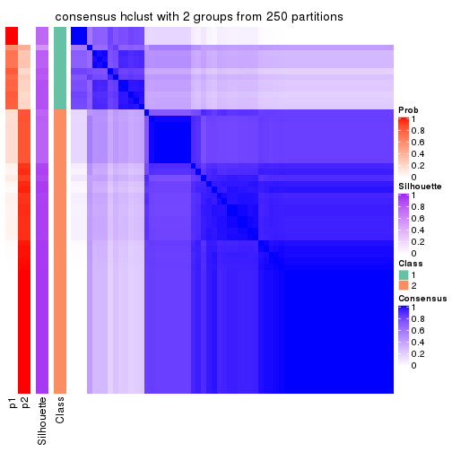
consensus_heatmap(res, k = 3)
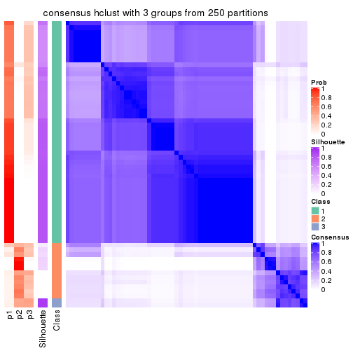
consensus_heatmap(res, k = 4)
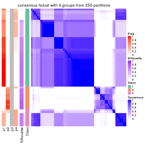
consensus_heatmap(res, k = 5)
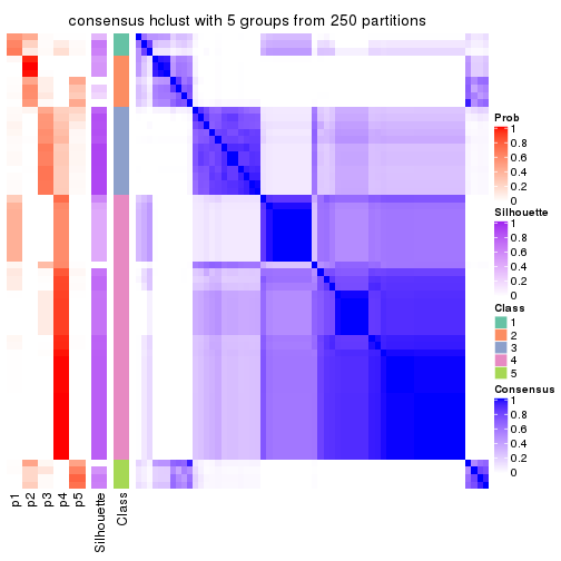
consensus_heatmap(res, k = 6)
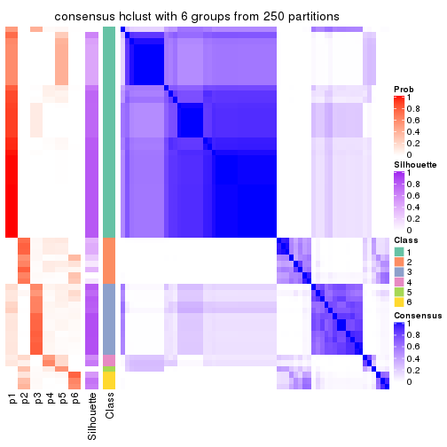
Heatmaps for the membership of samples in all partitions to see how consistent they are:
membership_heatmap(res, k = 2)
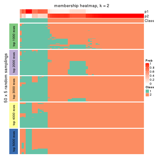
membership_heatmap(res, k = 3)
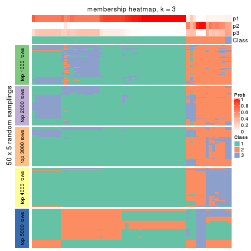
membership_heatmap(res, k = 4)
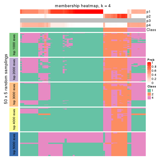
membership_heatmap(res, k = 5)
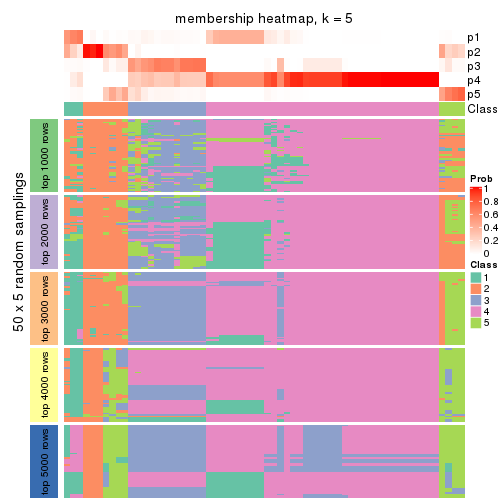
membership_heatmap(res, k = 6)
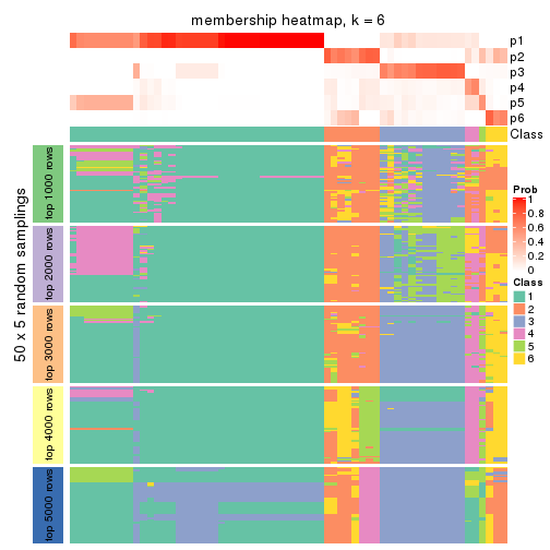
As soon as we have had the classes for columns, we can look for signatures which are significantly different between classes which can be candidate marks for certain classes. Following are the heatmaps for signatures.
Signature heatmaps where rows are scaled:
get_signatures(res, k = 2)
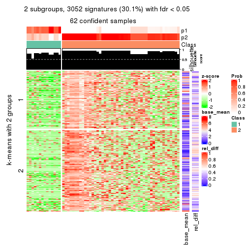
get_signatures(res, k = 3)
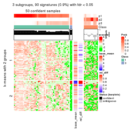
get_signatures(res, k = 4)
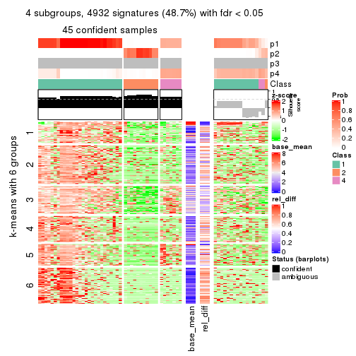
get_signatures(res, k = 5)
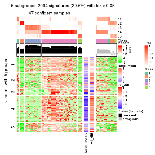
get_signatures(res, k = 6)
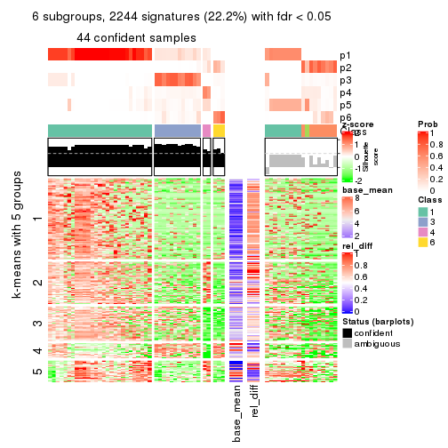
Signature heatmaps where rows are not scaled:
get_signatures(res, k = 2, scale_rows = FALSE)
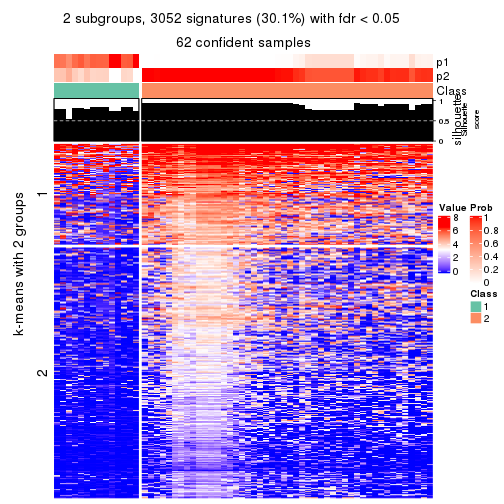
get_signatures(res, k = 3, scale_rows = FALSE)
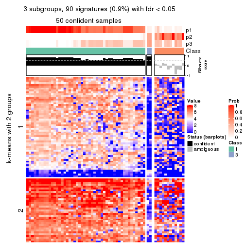
get_signatures(res, k = 4, scale_rows = FALSE)
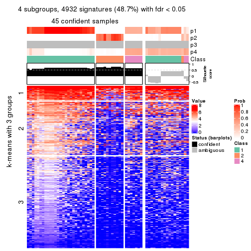
get_signatures(res, k = 5, scale_rows = FALSE)
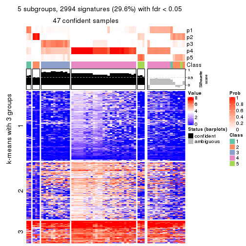
get_signatures(res, k = 6, scale_rows = FALSE)
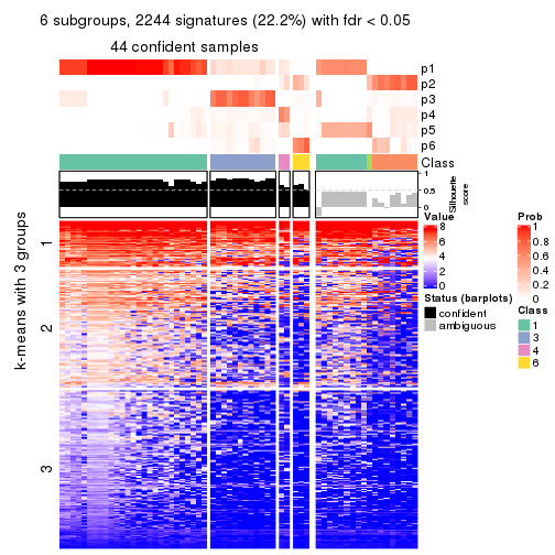
Compare the overlap of signatures from different k:
compare_signatures(res)
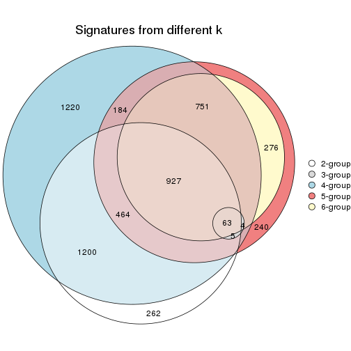
get_signature() returns a data frame invisibly. TO get the list of signatures, the function
call should be assigned to a variable explicitly. In following code, if plot argument is set
to FALSE, no heatmap is plotted while only the differential analysis is performed.
# code only for demonstration
tb = get_signature(res, k = ..., plot = FALSE)
An example of the output of tb is:
#>   which_row         fdr    mean_1    mean_2 scaled_mean_1 scaled_mean_2 km
#> 1        38 0.042760348  8.373488  9.131774    -0.5533452     0.5164555  1
#> 2        40 0.018707592  7.106213  8.469186    -0.6173731     0.5762149  1
#> 3        55 0.019134737 10.221463 11.207825    -0.6159697     0.5749050  1
#> 4        59 0.006059896  5.921854  7.869574    -0.6899429     0.6439467  1
#> 5        60 0.018055526  8.928898 10.211722    -0.6204761     0.5791110  1
#> 6        98 0.009384629 15.714769 14.887706     0.6635654    -0.6193277  2
...
The columns in tb are:
which_row: row indices corresponding to the input matrix.fdr: FDR for the differential test. mean_x: The mean value in group x.scaled_mean_x: The mean value in group x after rows are scaled.km: Row groups if k-means clustering is applied to rows.UMAP plot which shows how samples are separated.
dimension_reduction(res, k = 2, method = "UMAP")
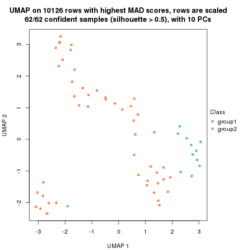
dimension_reduction(res, k = 3, method = "UMAP")
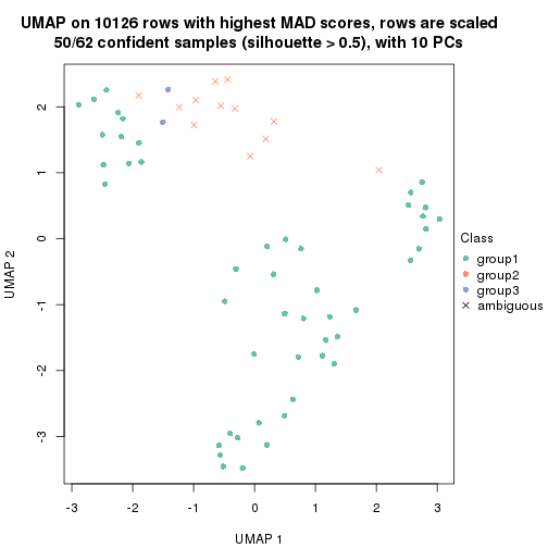
dimension_reduction(res, k = 4, method = "UMAP")
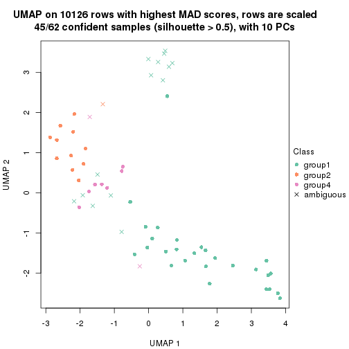
dimension_reduction(res, k = 5, method = "UMAP")
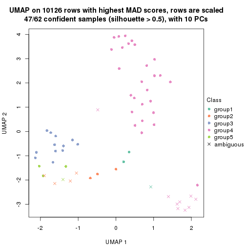
dimension_reduction(res, k = 6, method = "UMAP")
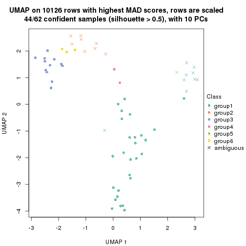
Following heatmap shows how subgroups are split when increasing k:
collect_classes(res)
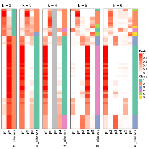
If matrix rows can be associated to genes, consider to use functional_enrichment(res,
...) to perform function enrichment for the signature genes. See this vignette for more detailed explanations.
The object with results only for a single top-value method and a single partition method can be extracted as:
res = res_list["MAD", "kmeans"]
# you can also extract it by
# res = res_list["MAD:kmeans"]
A summary of res and all the functions that can be applied to it:
res
#> A 'ConsensusPartition' object with k = 2, 3, 4, 5, 6.
#>   On a matrix with 10126 rows and 62 columns.
#>   Top rows (1000, 2000, 3000, 4000, 5000) are extracted by 'MAD' method.
#>   Subgroups are detected by 'kmeans' method.
#>   Performed in total 1250 partitions by row resampling.
#>   Best k for subgroups seems to be 4.
#>
#> Following methods can be applied to this 'ConsensusPartition' object:
#>  [1] "cola_report"             "collect_classes"         "collect_plots"
#>  [4] "collect_stats"           "colnames"                "compare_signatures"
#>  [7] "consensus_heatmap"       "dimension_reduction"     "functional_enrichment"
#> [10] "get_anno_col"            "get_anno"                "get_classes"
#> [13] "get_consensus"           "get_matrix"              "get_membership"
#> [16] "get_param"               "get_signatures"          "get_stats"
#> [19] "is_best_k"               "is_stable_k"             "membership_heatmap"
#> [22] "ncol"                    "nrow"                    "plot_ecdf"
#> [25] "rownames"                "select_partition_number" "show"
#> [28] "suggest_best_k"          "test_to_known_factors"
collect_plots() function collects all the plots made from res for all k (number of partitions)
into one single page to provide an easy and fast comparison between different k.
collect_plots(res)
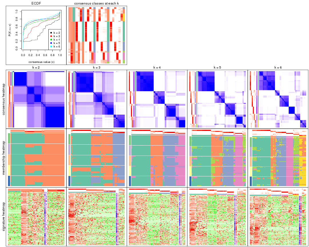
The plots are:
k and the heatmap of
predicted classes for each k.k.k.k.All the plots in panels can be made by individual functions and they are plotted later in this section.
select_partition_number() produces several plots showing different
statistics for choosing “optimized” k. There are following statistics:
k;k, the area increased is defined as \(A_k - A_{k-1}\).The detailed explanations of these statistics can be found in the cola vignette.
Generally speaking, lower PAC score, higher mean silhouette score or higher
concordance corresponds to better partition. Rand index and Jaccard index
measure how similar the current partition is compared to partition with k-1.
If they are too similar, we won't accept k is better than k-1.
select_partition_number(res)
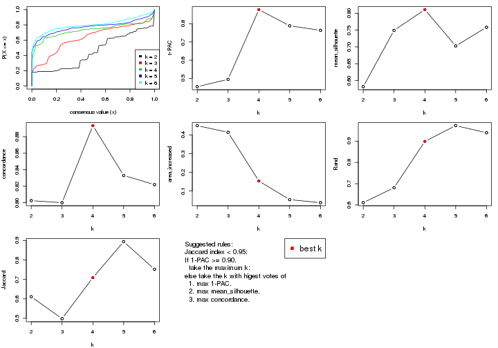
The numeric values for all these statistics can be obtained by get_stats().
get_stats(res)
#>   k 1-PAC mean_silhouette concordance area_increased  Rand Jaccard
#> 2 2 0.454           0.582       0.803         0.4497 0.611   0.611
#> 3 3 0.494           0.749       0.800         0.4139 0.681   0.498
#> 4 4 0.878           0.811       0.893         0.1535 0.899   0.709
#> 5 5 0.789           0.703       0.833         0.0540 0.973   0.895
#> 6 6 0.764           0.758       0.822         0.0377 0.940   0.752
suggest_best_k() suggests the best \(k\) based on these statistics. The rules are as follows:
suggest_best_k(res)
#> [1] 4
Following shows the table of the partitions (You need to click the show/hide
code output link to see it). The membership matrix (columns with name p*)
is inferred by
clue::cl_consensus()
function with the SE method. Basically the value in the membership matrix
represents the probability to belong to a certain group. The finall class
label for an item is determined with the group with highest probability it
belongs to.
In get_classes() function, the entropy is calculated from the membership
matrix and the silhouette score is calculated from the consensus matrix.
cbind(get_classes(res, k = 2), get_membership(res, k = 2))
#>            class entropy silhouette    p1    p2
#> SRR764776      2  0.9963      0.694 0.464 0.536
#> SRR764777      2  0.9963      0.694 0.464 0.536
#> SRR764778      2  0.9963      0.694 0.464 0.536
#> SRR764779      2  0.9963      0.694 0.464 0.536
#> SRR764780      2  0.9963      0.694 0.464 0.536
#> SRR764781      2  0.9963      0.694 0.464 0.536
#> SRR764782      2  0.9963      0.694 0.464 0.536
#> SRR764783      2  0.9963      0.694 0.464 0.536
#> SRR764784      2  0.9963      0.694 0.464 0.536
#> SRR764785      1  0.9963      0.920 0.536 0.464
#> SRR764786      1  0.9963      0.920 0.536 0.464
#> SRR764787      2  0.7883      0.607 0.236 0.764
#> SRR764788      2  0.9963      0.694 0.464 0.536
#> SRR764789      2  0.0376      0.426 0.004 0.996
#> SRR764790      1  0.9963      0.920 0.536 0.464
#> SRR764791      2  0.3274      0.481 0.060 0.940
#> SRR764792      2  0.9954      0.693 0.460 0.540
#> SRR764793      2  0.9963      0.694 0.464 0.536
#> SRR764794      2  0.4298      0.257 0.088 0.912
#> SRR764795      2  0.9963      0.694 0.464 0.536
#> SRR764796      2  0.9963      0.694 0.464 0.536
#> SRR764797      2  0.9963      0.694 0.464 0.536
#> SRR764798      2  0.9460      0.613 0.364 0.636
#> SRR764799      2  0.9963      0.694 0.464 0.536
#> SRR764800      2  0.9963      0.694 0.464 0.536
#> SRR764801      1  0.9996     -0.693 0.512 0.488
#> SRR764802      2  0.9963      0.694 0.464 0.536
#> SRR764803      2  0.9963      0.694 0.464 0.536
#> SRR764804      1  0.9963      0.920 0.536 0.464
#> SRR764805      1  0.9963      0.920 0.536 0.464
#> SRR764806      2  0.6048      0.115 0.148 0.852
#> SRR764807      1  0.9963      0.920 0.536 0.464
#> SRR764808      1  0.9963      0.920 0.536 0.464
#> SRR764809      1  0.9963      0.920 0.536 0.464
#> SRR764810      1  0.9963      0.920 0.536 0.464
#> SRR764811      1  0.9963      0.920 0.536 0.464
#> SRR764812      1  0.9963      0.920 0.536 0.464
#> SRR764813      1  0.9963      0.920 0.536 0.464
#> SRR764814      2  0.9963      0.694 0.464 0.536
#> SRR764815      2  0.5737      0.543 0.136 0.864
#> SRR764816      2  0.9963      0.694 0.464 0.536
#> SRR764817      2  0.9963      0.694 0.464 0.536
#> SRR1066622     2  0.0000      0.421 0.000 1.000
#> SRR1066623     2  0.0000      0.421 0.000 1.000
#> SRR1066624     2  0.9963      0.694 0.464 0.536
#> SRR1066625     2  0.8661      0.632 0.288 0.712
#> SRR1066626     2  0.2236      0.361 0.036 0.964
#> SRR1066627     2  0.0000      0.421 0.000 1.000
#> SRR1066628     2  0.0000      0.421 0.000 1.000
#> SRR1066629     2  0.0000      0.421 0.000 1.000
#> SRR1066630     1  0.9963      0.920 0.536 0.464
#> SRR1066631     2  0.0000      0.421 0.000 1.000
#> SRR1066632     2  0.5946      0.129 0.144 0.856
#> SRR1066633     2  0.5946      0.129 0.144 0.856
#> SRR1066634     2  0.5946      0.129 0.144 0.856
#> SRR1066635     1  0.9963      0.920 0.536 0.464
#> SRR1066636     2  0.5946      0.129 0.144 0.856
#> SRR1066637     2  0.5946      0.129 0.144 0.856
#> SRR1066638     2  0.5946      0.129 0.144 0.856
#> SRR1066639     2  0.8955     -0.466 0.312 0.688
#> SRR1066640     2  0.5946      0.129 0.144 0.856
#> SRR1066641     1  0.9963      0.920 0.536 0.464
cbind(get_classes(res, k = 3), get_membership(res, k = 3))
#>            class entropy silhouette    p1    p2    p3
#> SRR764776      1  0.0237     0.9386 0.996 0.004 0.000
#> SRR764777      1  0.0237     0.9386 0.996 0.004 0.000
#> SRR764778      1  0.0237     0.9386 0.996 0.004 0.000
#> SRR764779      1  0.0237     0.9386 0.996 0.004 0.000
#> SRR764780      1  0.0000     0.9387 1.000 0.000 0.000
#> SRR764781      1  0.0000     0.9387 1.000 0.000 0.000
#> SRR764782      1  0.1031     0.9216 0.976 0.024 0.000
#> SRR764783      1  0.0000     0.9387 1.000 0.000 0.000
#> SRR764784      1  0.1031     0.9216 0.976 0.024 0.000
#> SRR764785      3  0.4654     0.7786 0.000 0.208 0.792
#> SRR764786      3  0.4452     0.7934 0.000 0.192 0.808
#> SRR764787      2  0.6608     0.4864 0.432 0.560 0.008
#> SRR764788      1  0.0000     0.9387 1.000 0.000 0.000
#> SRR764789      2  0.4978     0.6741 0.216 0.780 0.004
#> SRR764790      3  0.2261     0.8735 0.000 0.068 0.932
#> SRR764791      2  0.5928     0.6381 0.296 0.696 0.008
#> SRR764792      2  0.6308     0.3635 0.492 0.508 0.000
#> SRR764793      1  0.5882     0.1505 0.652 0.348 0.000
#> SRR764794      2  0.4897     0.6776 0.172 0.812 0.016
#> SRR764795      1  0.1031     0.9216 0.976 0.024 0.000
#> SRR764796      1  0.1289     0.9124 0.968 0.032 0.000
#> SRR764797      1  0.0000     0.9387 1.000 0.000 0.000
#> SRR764798      2  0.8370     0.2594 0.416 0.500 0.084
#> SRR764799      1  0.0592     0.9340 0.988 0.012 0.000
#> SRR764800      1  0.0424     0.9366 0.992 0.008 0.000
#> SRR764801      1  0.7831     0.0672 0.540 0.404 0.056
#> SRR764802      1  0.0000     0.9387 1.000 0.000 0.000
#> SRR764803      1  0.0000     0.9387 1.000 0.000 0.000
#> SRR764804      3  0.0237     0.9057 0.000 0.004 0.996
#> SRR764805      3  0.4062     0.7900 0.000 0.164 0.836
#> SRR764806      2  0.7605     0.6011 0.124 0.684 0.192
#> SRR764807      3  0.0592     0.9044 0.000 0.012 0.988
#> SRR764808      3  0.0592     0.9044 0.000 0.012 0.988
#> SRR764809      3  0.3941     0.7984 0.000 0.156 0.844
#> SRR764810      3  0.2356     0.8684 0.000 0.072 0.928
#> SRR764811      3  0.0237     0.9057 0.000 0.004 0.996
#> SRR764812      3  0.0237     0.9057 0.000 0.004 0.996
#> SRR764813      3  0.0000     0.9062 0.000 0.000 1.000
#> SRR764814      1  0.0592     0.9340 0.988 0.012 0.000
#> SRR764815      2  0.6314     0.5294 0.392 0.604 0.004
#> SRR764816      1  0.0592     0.9340 0.988 0.012 0.000
#> SRR764817      1  0.0592     0.9340 0.988 0.012 0.000
#> SRR1066622     2  0.5816     0.6607 0.224 0.752 0.024
#> SRR1066623     2  0.5816     0.6607 0.224 0.752 0.024
#> SRR1066624     1  0.0237     0.9361 0.996 0.004 0.000
#> SRR1066625     2  0.5244     0.6538 0.240 0.756 0.004
#> SRR1066626     2  0.5816     0.6607 0.224 0.752 0.024
#> SRR1066627     2  0.5816     0.6607 0.224 0.752 0.024
#> SRR1066628     2  0.5816     0.6607 0.224 0.752 0.024
#> SRR1066629     2  0.5816     0.6607 0.224 0.752 0.024
#> SRR1066630     3  0.4654     0.7801 0.000 0.208 0.792
#> SRR1066631     2  0.5816     0.6607 0.224 0.752 0.024
#> SRR1066632     2  0.7361     0.6136 0.124 0.704 0.172
#> SRR1066633     2  0.7605     0.6011 0.124 0.684 0.192
#> SRR1066634     2  0.7034     0.6243 0.124 0.728 0.148
#> SRR1066635     2  0.5968     0.3419 0.000 0.636 0.364
#> SRR1066636     2  0.7605     0.6011 0.124 0.684 0.192
#> SRR1066637     2  0.7605     0.6011 0.124 0.684 0.192
#> SRR1066638     2  0.7510     0.6065 0.124 0.692 0.184
#> SRR1066639     2  0.6487     0.4984 0.032 0.700 0.268
#> SRR1066640     2  0.7605     0.6011 0.124 0.684 0.192
#> SRR1066641     3  0.0000     0.9062 0.000 0.000 1.000
cbind(get_classes(res, k = 4), get_membership(res, k = 4))
#>            class entropy silhouette    p1    p2    p3    p4
#> SRR764776      1  0.0188      0.962 0.996 0.000 0.000 0.004
#> SRR764777      1  0.0188      0.962 0.996 0.000 0.000 0.004
#> SRR764778      1  0.0188      0.962 0.996 0.000 0.000 0.004
#> SRR764779      1  0.0188      0.962 0.996 0.000 0.000 0.004
#> SRR764780      1  0.0000      0.962 1.000 0.000 0.000 0.000
#> SRR764781      1  0.0000      0.962 1.000 0.000 0.000 0.000
#> SRR764782      1  0.2282      0.914 0.924 0.000 0.024 0.052
#> SRR764783      1  0.0000      0.962 1.000 0.000 0.000 0.000
#> SRR764784      1  0.2197      0.918 0.928 0.000 0.024 0.048
#> SRR764785      2  0.4677      0.673 0.000 0.680 0.004 0.316
#> SRR764786      2  0.4456      0.714 0.000 0.716 0.004 0.280
#> SRR764787      4  0.7608      0.236 0.200 0.000 0.392 0.408
#> SRR764788      1  0.0336      0.961 0.992 0.000 0.000 0.008
#> SRR764789      4  0.5526      0.501 0.020 0.000 0.416 0.564
#> SRR764790      2  0.1389      0.866 0.000 0.952 0.000 0.048
#> SRR764791      4  0.5636      0.479 0.024 0.000 0.424 0.552
#> SRR764792      3  0.7666     -0.325 0.212 0.000 0.400 0.388
#> SRR764793      1  0.6058      0.548 0.684 0.000 0.136 0.180
#> SRR764794      4  0.5352      0.505 0.016 0.000 0.388 0.596
#> SRR764795      1  0.2197      0.918 0.928 0.000 0.024 0.048
#> SRR764796      1  0.2300      0.912 0.924 0.000 0.028 0.048
#> SRR764797      1  0.0336      0.961 0.992 0.000 0.000 0.008
#> SRR764798      3  0.2124      0.810 0.068 0.000 0.924 0.008
#> SRR764799      1  0.0804      0.954 0.980 0.000 0.012 0.008
#> SRR764800      1  0.0336      0.961 0.992 0.000 0.000 0.008
#> SRR764801      3  0.2342      0.795 0.080 0.000 0.912 0.008
#> SRR764802      1  0.0188      0.962 0.996 0.000 0.000 0.004
#> SRR764803      1  0.0188      0.962 0.996 0.000 0.000 0.004
#> SRR764804      2  0.0657      0.871 0.000 0.984 0.004 0.012
#> SRR764805      2  0.4883      0.636 0.000 0.696 0.288 0.016
#> SRR764806      3  0.0469      0.866 0.000 0.012 0.988 0.000
#> SRR764807      2  0.1389      0.866 0.000 0.952 0.000 0.048
#> SRR764808      2  0.1389      0.866 0.000 0.952 0.000 0.048
#> SRR764809      2  0.4502      0.704 0.000 0.748 0.236 0.016
#> SRR764810      2  0.2796      0.832 0.000 0.892 0.092 0.016
#> SRR764811      2  0.0376      0.872 0.000 0.992 0.004 0.004
#> SRR764812      2  0.0524      0.872 0.000 0.988 0.004 0.008
#> SRR764813      2  0.0188      0.872 0.000 0.996 0.004 0.000
#> SRR764814      1  0.0804      0.954 0.980 0.000 0.012 0.008
#> SRR764815      3  0.6691      0.230 0.152 0.000 0.612 0.236
#> SRR764816      1  0.0804      0.954 0.980 0.000 0.012 0.008
#> SRR764817      1  0.0804      0.954 0.980 0.000 0.012 0.008
#> SRR1066622     4  0.3080      0.831 0.024 0.000 0.096 0.880
#> SRR1066623     4  0.3080      0.831 0.024 0.000 0.096 0.880
#> SRR1066624     1  0.0000      0.962 1.000 0.000 0.000 0.000
#> SRR1066625     4  0.3080      0.831 0.024 0.000 0.096 0.880
#> SRR1066626     4  0.3080      0.831 0.024 0.000 0.096 0.880
#> SRR1066627     4  0.3080      0.831 0.024 0.000 0.096 0.880
#> SRR1066628     4  0.3080      0.831 0.024 0.000 0.096 0.880
#> SRR1066629     4  0.3080      0.831 0.024 0.000 0.096 0.880
#> SRR1066630     2  0.4741      0.657 0.000 0.668 0.004 0.328
#> SRR1066631     4  0.3080      0.831 0.024 0.000 0.096 0.880
#> SRR1066632     3  0.0000      0.874 0.000 0.000 1.000 0.000
#> SRR1066633     3  0.0000      0.874 0.000 0.000 1.000 0.000
#> SRR1066634     3  0.0188      0.872 0.000 0.000 0.996 0.004
#> SRR1066635     3  0.1767      0.832 0.000 0.044 0.944 0.012
#> SRR1066636     3  0.0000      0.874 0.000 0.000 1.000 0.000
#> SRR1066637     3  0.0000      0.874 0.000 0.000 1.000 0.000
#> SRR1066638     3  0.0000      0.874 0.000 0.000 1.000 0.000
#> SRR1066639     3  0.0000      0.874 0.000 0.000 1.000 0.000
#> SRR1066640     3  0.0000      0.874 0.000 0.000 1.000 0.000
#> SRR1066641     2  0.0188      0.872 0.000 0.996 0.004 0.000
cbind(get_classes(res, k = 5), get_membership(res, k = 5))
#>            class entropy silhouette    p1    p2    p3    p4    p5
#> SRR764776      1  0.0162      0.919 0.996 0.000 0.000 0.000 0.004
#> SRR764777      1  0.0162      0.919 0.996 0.000 0.000 0.000 0.004
#> SRR764778      1  0.0162      0.919 0.996 0.000 0.000 0.000 0.004
#> SRR764779      1  0.0162      0.919 0.996 0.000 0.000 0.000 0.004
#> SRR764780      1  0.0000      0.919 1.000 0.000 0.000 0.000 0.000
#> SRR764781      1  0.0000      0.919 1.000 0.000 0.000 0.000 0.000
#> SRR764782      1  0.3912      0.802 0.824 0.000 0.016 0.084 0.076
#> SRR764783      1  0.0000      0.919 1.000 0.000 0.000 0.000 0.000
#> SRR764784      1  0.3968      0.797 0.820 0.000 0.016 0.088 0.076
#> SRR764785      5  0.5434     -0.315 0.000 0.336 0.000 0.076 0.588
#> SRR764786      2  0.5604      0.392 0.000 0.472 0.000 0.072 0.456
#> SRR764787      5  0.8235      0.476 0.128 0.000 0.224 0.292 0.356
#> SRR764788      1  0.2228      0.872 0.908 0.000 0.004 0.012 0.076
#> SRR764789      4  0.6938     -0.442 0.008 0.000 0.244 0.400 0.348
#> SRR764790      2  0.4434      0.616 0.000 0.640 0.004 0.008 0.348
#> SRR764791      4  0.7186     -0.476 0.020 0.000 0.244 0.392 0.344
#> SRR764792      5  0.8300      0.476 0.136 0.000 0.236 0.280 0.348
#> SRR764793      1  0.7384      0.123 0.512 0.000 0.080 0.172 0.236
#> SRR764794      5  0.6617      0.338 0.004 0.000 0.200 0.328 0.468
#> SRR764795      1  0.3852      0.805 0.828 0.000 0.016 0.084 0.072
#> SRR764796      1  0.4058      0.791 0.816 0.000 0.020 0.092 0.072
#> SRR764797      1  0.1106      0.907 0.964 0.000 0.000 0.012 0.024
#> SRR764798      3  0.2569      0.825 0.040 0.000 0.892 0.000 0.068
#> SRR764799      1  0.1043      0.906 0.960 0.000 0.000 0.000 0.040
#> SRR764800      1  0.0609      0.913 0.980 0.000 0.000 0.000 0.020
#> SRR764801      3  0.2569      0.825 0.040 0.000 0.892 0.000 0.068
#> SRR764802      1  0.0162      0.919 0.996 0.000 0.000 0.004 0.000
#> SRR764803      1  0.0324      0.918 0.992 0.000 0.000 0.004 0.004
#> SRR764804      2  0.1484      0.740 0.000 0.944 0.008 0.000 0.048
#> SRR764805      2  0.5271      0.600 0.000 0.680 0.152 0.000 0.168
#> SRR764806      3  0.1430      0.851 0.000 0.004 0.944 0.000 0.052
#> SRR764807      2  0.4156      0.656 0.000 0.700 0.004 0.008 0.288
#> SRR764808      2  0.4156      0.656 0.000 0.700 0.004 0.008 0.288
#> SRR764809      2  0.5224      0.605 0.000 0.684 0.140 0.000 0.176
#> SRR764810      2  0.3888      0.678 0.000 0.788 0.032 0.004 0.176
#> SRR764811      2  0.2011      0.729 0.000 0.908 0.004 0.000 0.088
#> SRR764812      2  0.0865      0.744 0.000 0.972 0.004 0.000 0.024
#> SRR764813      2  0.0671      0.744 0.000 0.980 0.004 0.000 0.016
#> SRR764814      1  0.1043      0.906 0.960 0.000 0.000 0.000 0.040
#> SRR764815      3  0.7253     -0.289 0.068 0.000 0.456 0.124 0.352
#> SRR764816      1  0.1043      0.906 0.960 0.000 0.000 0.000 0.040
#> SRR764817      1  0.1043      0.906 0.960 0.000 0.000 0.000 0.040
#> SRR1066622     4  0.0794      0.810 0.000 0.000 0.028 0.972 0.000
#> SRR1066623     4  0.0794      0.810 0.000 0.000 0.028 0.972 0.000
#> SRR1066624     1  0.0290      0.918 0.992 0.000 0.000 0.008 0.000
#> SRR1066625     4  0.0794      0.810 0.000 0.000 0.028 0.972 0.000
#> SRR1066626     4  0.0794      0.810 0.000 0.000 0.028 0.972 0.000
#> SRR1066627     4  0.0794      0.810 0.000 0.000 0.028 0.972 0.000
#> SRR1066628     4  0.0794      0.810 0.000 0.000 0.028 0.972 0.000
#> SRR1066629     4  0.0794      0.810 0.000 0.000 0.028 0.972 0.000
#> SRR1066630     2  0.6386      0.444 0.000 0.492 0.000 0.188 0.320
#> SRR1066631     4  0.0794      0.810 0.000 0.000 0.028 0.972 0.000
#> SRR1066632     3  0.1502      0.854 0.000 0.000 0.940 0.004 0.056
#> SRR1066633     3  0.0566      0.877 0.000 0.000 0.984 0.004 0.012
#> SRR1066634     3  0.1768      0.845 0.000 0.000 0.924 0.004 0.072
#> SRR1066635     3  0.3495      0.726 0.000 0.032 0.816 0.000 0.152
#> SRR1066636     3  0.0451      0.877 0.000 0.000 0.988 0.004 0.008
#> SRR1066637     3  0.0324      0.877 0.000 0.000 0.992 0.004 0.004
#> SRR1066638     3  0.1571      0.850 0.000 0.000 0.936 0.004 0.060
#> SRR1066639     3  0.0162      0.877 0.000 0.000 0.996 0.004 0.000
#> SRR1066640     3  0.0162      0.877 0.000 0.000 0.996 0.004 0.000
#> SRR1066641     2  0.0771      0.744 0.000 0.976 0.004 0.000 0.020
cbind(get_classes(res, k = 6), get_membership(res, k = 6))
#>            class entropy silhouette    p1    p2    p3    p4    p5    p6
#> SRR764776      1  0.0000      0.870 1.000 0.000 0.000 0.000 0.000 0.000
#> SRR764777      1  0.0000      0.870 1.000 0.000 0.000 0.000 0.000 0.000
#> SRR764778      1  0.0000      0.870 1.000 0.000 0.000 0.000 0.000 0.000
#> SRR764779      1  0.0000      0.870 1.000 0.000 0.000 0.000 0.000 0.000
#> SRR764780      1  0.0547      0.870 0.980 0.000 0.000 0.000 0.020 0.000
#> SRR764781      1  0.0547      0.870 0.980 0.000 0.000 0.000 0.020 0.000
#> SRR764782      1  0.4667      0.593 0.684 0.008 0.012 0.044 0.252 0.000
#> SRR764783      1  0.0713      0.869 0.972 0.000 0.000 0.000 0.028 0.000
#> SRR764784      1  0.4598      0.615 0.696 0.008 0.012 0.044 0.240 0.000
#> SRR764785      2  0.4693      0.360 0.000 0.532 0.000 0.024 0.432 0.012
#> SRR764786      2  0.4951      0.542 0.000 0.660 0.000 0.024 0.252 0.064
#> SRR764787      5  0.6150      0.762 0.104 0.020 0.132 0.104 0.640 0.000
#> SRR764788      1  0.3281      0.729 0.784 0.004 0.012 0.000 0.200 0.000
#> SRR764789      5  0.5652      0.730 0.020 0.016 0.144 0.176 0.644 0.000
#> SRR764790      2  0.2597      0.566 0.000 0.824 0.000 0.000 0.000 0.176
#> SRR764791      5  0.5807      0.761 0.056 0.000 0.176 0.144 0.624 0.000
#> SRR764792      5  0.5840      0.767 0.096 0.004 0.164 0.092 0.644 0.000
#> SRR764793      5  0.5811      0.186 0.412 0.008 0.032 0.064 0.484 0.000
#> SRR764794      5  0.5376      0.450 0.004 0.152 0.084 0.072 0.688 0.000
#> SRR764795      1  0.4396      0.646 0.716 0.008 0.012 0.036 0.228 0.000
#> SRR764796      1  0.4418      0.639 0.712 0.004 0.012 0.044 0.228 0.000
#> SRR764797      1  0.1753      0.842 0.912 0.004 0.000 0.000 0.084 0.000
#> SRR764798      3  0.4742      0.744 0.048 0.040 0.752 0.000 0.136 0.024
#> SRR764799      1  0.2687      0.802 0.872 0.024 0.000 0.000 0.092 0.012
#> SRR764800      1  0.1219      0.848 0.948 0.004 0.000 0.000 0.048 0.000
#> SRR764801      3  0.4742      0.744 0.048 0.040 0.752 0.000 0.136 0.024
#> SRR764802      1  0.1010      0.866 0.960 0.004 0.000 0.000 0.036 0.000
#> SRR764803      1  0.1152      0.863 0.952 0.004 0.000 0.000 0.044 0.000
#> SRR764804      6  0.3329      0.671 0.000 0.236 0.004 0.000 0.004 0.756
#> SRR764805      6  0.2255      0.616 0.000 0.016 0.088 0.000 0.004 0.892
#> SRR764806      3  0.2095      0.865 0.000 0.016 0.916 0.000 0.028 0.040
#> SRR764807      2  0.3151      0.497 0.000 0.748 0.000 0.000 0.000 0.252
#> SRR764808      2  0.3126      0.504 0.000 0.752 0.000 0.000 0.000 0.248
#> SRR764809      6  0.2255      0.605 0.000 0.004 0.088 0.000 0.016 0.892
#> SRR764810      6  0.1204      0.647 0.000 0.004 0.016 0.004 0.016 0.960
#> SRR764811      6  0.3739      0.654 0.000 0.220 0.004 0.004 0.020 0.752
#> SRR764812      6  0.3468      0.648 0.000 0.284 0.004 0.000 0.000 0.712
#> SRR764813      6  0.3905      0.553 0.000 0.356 0.004 0.000 0.004 0.636
#> SRR764814      1  0.2415      0.815 0.888 0.016 0.000 0.000 0.084 0.012
#> SRR764815      5  0.5113      0.669 0.048 0.008 0.252 0.032 0.660 0.000
#> SRR764816      1  0.2415      0.815 0.888 0.016 0.000 0.000 0.084 0.012
#> SRR764817      1  0.2415      0.815 0.888 0.016 0.000 0.000 0.084 0.012
#> SRR1066622     4  0.0405      0.999 0.004 0.000 0.008 0.988 0.000 0.000
#> SRR1066623     4  0.0551      0.997 0.004 0.004 0.008 0.984 0.000 0.000
#> SRR1066624     1  0.1124      0.862 0.956 0.008 0.000 0.036 0.000 0.000
#> SRR1066625     4  0.0405      0.999 0.004 0.000 0.008 0.988 0.000 0.000
#> SRR1066626     4  0.0551      0.997 0.004 0.004 0.008 0.984 0.000 0.000
#> SRR1066627     4  0.0405      0.999 0.004 0.000 0.008 0.988 0.000 0.000
#> SRR1066628     4  0.0405      0.999 0.004 0.000 0.008 0.988 0.000 0.000
#> SRR1066629     4  0.0405      0.999 0.004 0.000 0.008 0.988 0.000 0.000
#> SRR1066630     2  0.5968      0.528 0.000 0.624 0.000 0.148 0.096 0.132
#> SRR1066631     4  0.0405      0.999 0.004 0.000 0.008 0.988 0.000 0.000
#> SRR1066632     3  0.2520      0.827 0.000 0.008 0.872 0.000 0.108 0.012
#> SRR1066633     3  0.0725      0.885 0.000 0.012 0.976 0.000 0.012 0.000
#> SRR1066634     3  0.2191      0.824 0.000 0.000 0.876 0.000 0.120 0.004
#> SRR1066635     3  0.3636      0.748 0.000 0.012 0.764 0.000 0.016 0.208
#> SRR1066636     3  0.0725      0.884 0.000 0.012 0.976 0.000 0.012 0.000
#> SRR1066637     3  0.0146      0.885 0.000 0.000 0.996 0.000 0.004 0.000
#> SRR1066638     3  0.2006      0.833 0.000 0.000 0.892 0.000 0.104 0.004
#> SRR1066639     3  0.0665      0.885 0.000 0.008 0.980 0.000 0.004 0.008
#> SRR1066640     3  0.0291      0.884 0.000 0.000 0.992 0.000 0.004 0.004
#> SRR1066641     6  0.4577      0.466 0.000 0.396 0.004 0.004 0.024 0.572
Heatmaps for the consensus matrix. It visualizes the probability of two samples to be in a same group.
consensus_heatmap(res, k = 2)
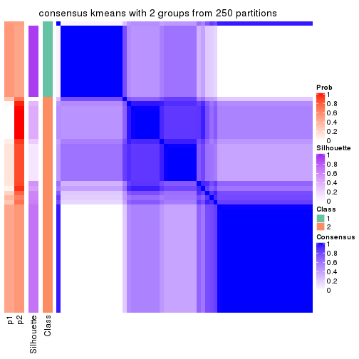
consensus_heatmap(res, k = 3)
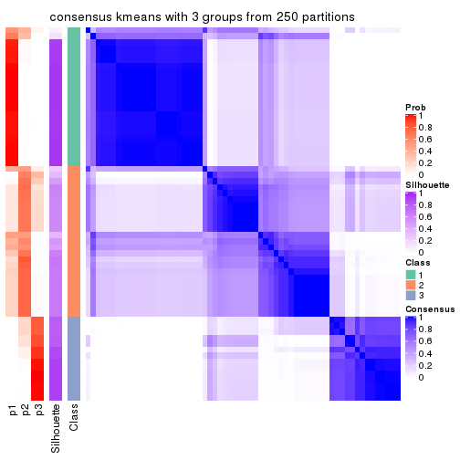
consensus_heatmap(res, k = 4)
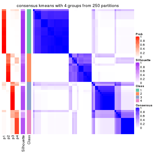
consensus_heatmap(res, k = 5)
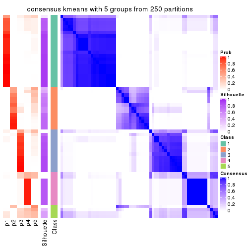
consensus_heatmap(res, k = 6)
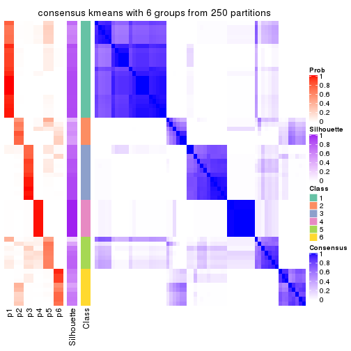
Heatmaps for the membership of samples in all partitions to see how consistent they are:
membership_heatmap(res, k = 2)
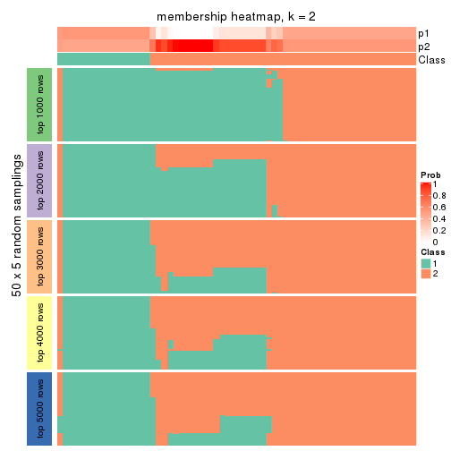
membership_heatmap(res, k = 3)
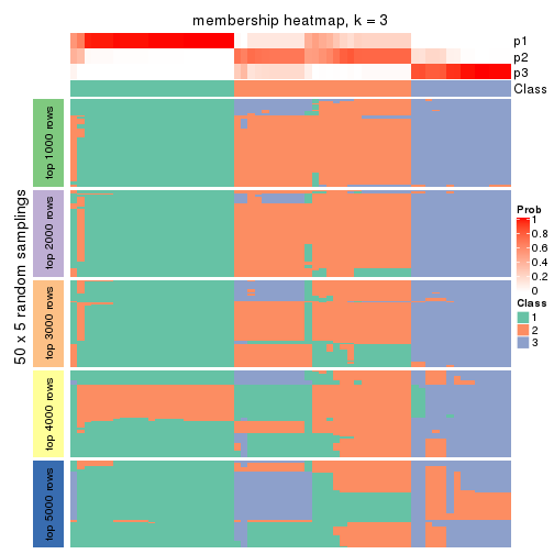
membership_heatmap(res, k = 4)
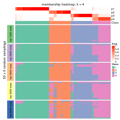
membership_heatmap(res, k = 5)
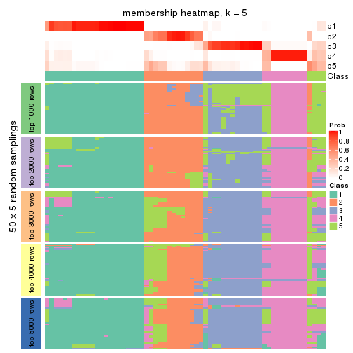
membership_heatmap(res, k = 6)
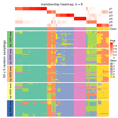
As soon as we have had the classes for columns, we can look for signatures which are significantly different between classes which can be candidate marks for certain classes. Following are the heatmaps for signatures.
Signature heatmaps where rows are scaled:
get_signatures(res, k = 2)
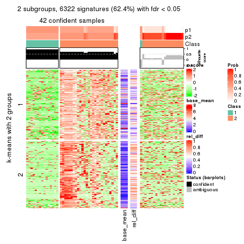
get_signatures(res, k = 3)
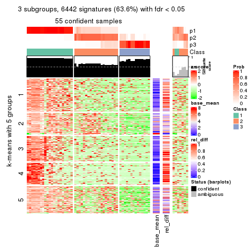
get_signatures(res, k = 4)
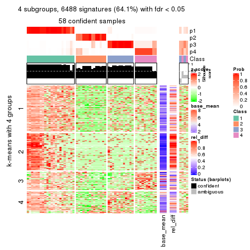
get_signatures(res, k = 5)
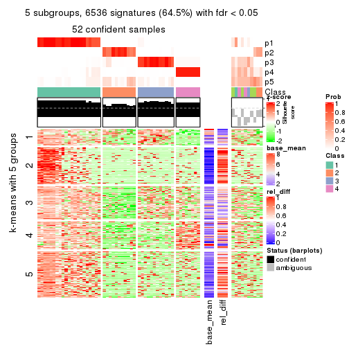
get_signatures(res, k = 6)
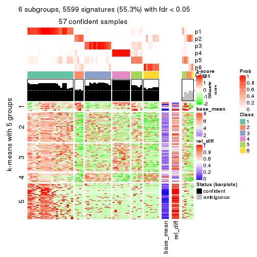
Signature heatmaps where rows are not scaled:
get_signatures(res, k = 2, scale_rows = FALSE)
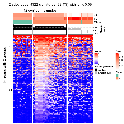
get_signatures(res, k = 3, scale_rows = FALSE)
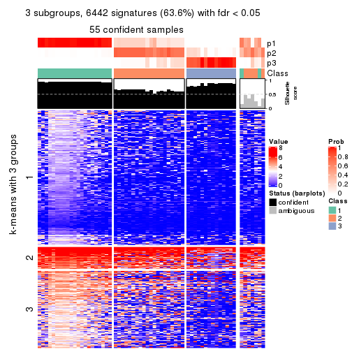
get_signatures(res, k = 4, scale_rows = FALSE)
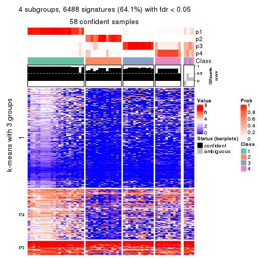
get_signatures(res, k = 5, scale_rows = FALSE)
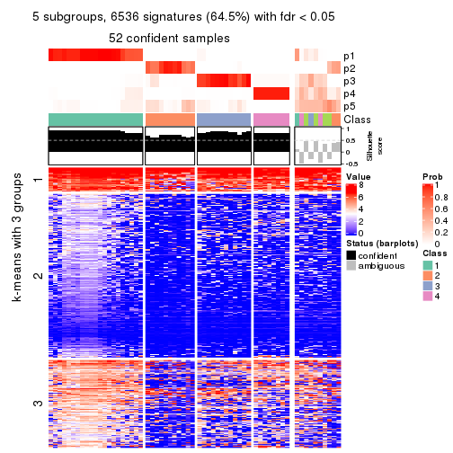
get_signatures(res, k = 6, scale_rows = FALSE)
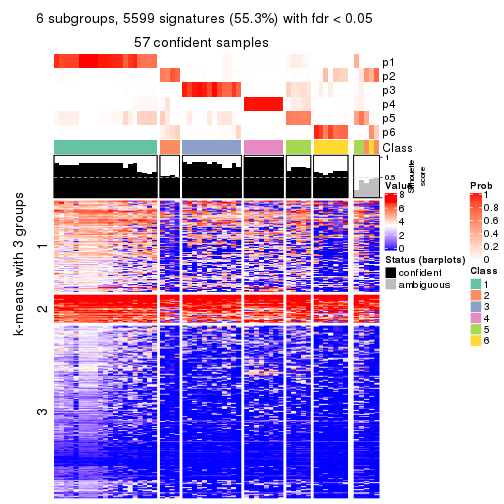
Compare the overlap of signatures from different k:
compare_signatures(res)
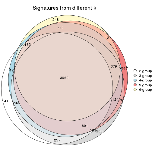
get_signature() returns a data frame invisibly. TO get the list of signatures, the function
call should be assigned to a variable explicitly. In following code, if plot argument is set
to FALSE, no heatmap is plotted while only the differential analysis is performed.
# code only for demonstration
tb = get_signature(res, k = ..., plot = FALSE)
An example of the output of tb is:
#>   which_row         fdr    mean_1    mean_2 scaled_mean_1 scaled_mean_2 km
#> 1        38 0.042760348  8.373488  9.131774    -0.5533452     0.5164555  1
#> 2        40 0.018707592  7.106213  8.469186    -0.6173731     0.5762149  1
#> 3        55 0.019134737 10.221463 11.207825    -0.6159697     0.5749050  1
#> 4        59 0.006059896  5.921854  7.869574    -0.6899429     0.6439467  1
#> 5        60 0.018055526  8.928898 10.211722    -0.6204761     0.5791110  1
#> 6        98 0.009384629 15.714769 14.887706     0.6635654    -0.6193277  2
...
The columns in tb are:
which_row: row indices corresponding to the input matrix.fdr: FDR for the differential test. mean_x: The mean value in group x.scaled_mean_x: The mean value in group x after rows are scaled.km: Row groups if k-means clustering is applied to rows.UMAP plot which shows how samples are separated.
dimension_reduction(res, k = 2, method = "UMAP")
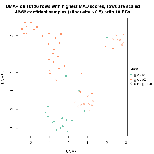
dimension_reduction(res, k = 3, method = "UMAP")
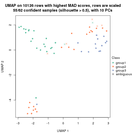
dimension_reduction(res, k = 4, method = "UMAP")
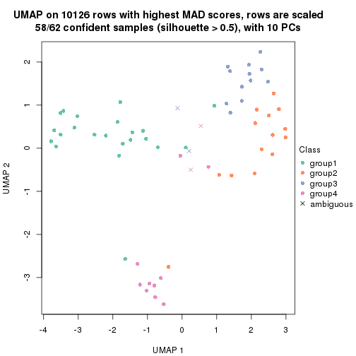
dimension_reduction(res, k = 5, method = "UMAP")
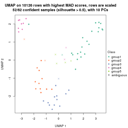
dimension_reduction(res, k = 6, method = "UMAP")

Following heatmap shows how subgroups are split when increasing k:
collect_classes(res)
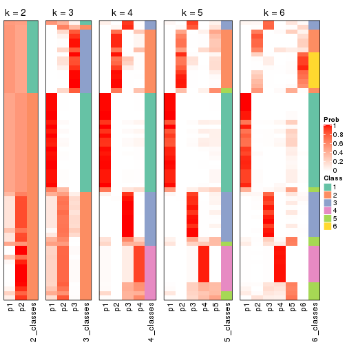
If matrix rows can be associated to genes, consider to use functional_enrichment(res,
...) to perform function enrichment for the signature genes. See this vignette for more detailed explanations.
The object with results only for a single top-value method and a single partition method can be extracted as:
res = res_list["MAD", "skmeans"]
# you can also extract it by
# res = res_list["MAD:skmeans"]
A summary of res and all the functions that can be applied to it:
res
#> A 'ConsensusPartition' object with k = 2, 3, 4, 5, 6.
#>   On a matrix with 10126 rows and 62 columns.
#>   Top rows (1000, 2000, 3000, 4000, 5000) are extracted by 'MAD' method.
#>   Subgroups are detected by 'skmeans' method.
#>   Performed in total 1250 partitions by row resampling.
#>   Best k for subgroups seems to be 2.
#>
#> Following methods can be applied to this 'ConsensusPartition' object:
#>  [1] "cola_report"             "collect_classes"         "collect_plots"
#>  [4] "collect_stats"           "colnames"                "compare_signatures"
#>  [7] "consensus_heatmap"       "dimension_reduction"     "functional_enrichment"
#> [10] "get_anno_col"            "get_anno"                "get_classes"
#> [13] "get_consensus"           "get_matrix"              "get_membership"
#> [16] "get_param"               "get_signatures"          "get_stats"
#> [19] "is_best_k"               "is_stable_k"             "membership_heatmap"
#> [22] "ncol"                    "nrow"                    "plot_ecdf"
#> [25] "rownames"                "select_partition_number" "show"
#> [28] "suggest_best_k"          "test_to_known_factors"
collect_plots() function collects all the plots made from res for all k (number of partitions)
into one single page to provide an easy and fast comparison between different k.
collect_plots(res)
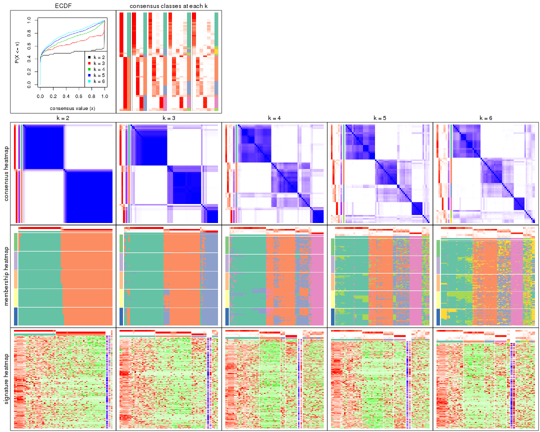
The plots are:
k and the heatmap of
predicted classes for each k.k.k.k.All the plots in panels can be made by individual functions and they are plotted later in this section.
select_partition_number() produces several plots showing different
statistics for choosing “optimized” k. There are following statistics:
k;k, the area increased is defined as \(A_k - A_{k-1}\).The detailed explanations of these statistics can be found in the cola vignette.
Generally speaking, lower PAC score, higher mean silhouette score or higher
concordance corresponds to better partition. Rand index and Jaccard index
measure how similar the current partition is compared to partition with k-1.
If they are too similar, we won't accept k is better than k-1.
select_partition_number(res)

The numeric values for all these statistics can be obtained by get_stats().
get_stats(res)
#>   k 1-PAC mean_silhouette concordance area_increased  Rand Jaccard
#> 2 2 1.000           0.963       0.986         0.5045 0.497   0.497
#> 3 3 0.847           0.844       0.937         0.2840 0.835   0.675
#> 4 4 0.647           0.671       0.834         0.1201 0.864   0.646
#> 5 5 0.646           0.669       0.794         0.0624 0.922   0.736
#> 6 6 0.646           0.600       0.726         0.0367 0.974   0.891
suggest_best_k() suggests the best \(k\) based on these statistics. The rules are as follows:
suggest_best_k(res)
#> [1] 2
Following shows the table of the partitions (You need to click the show/hide
code output link to see it). The membership matrix (columns with name p*)
is inferred by
clue::cl_consensus()
function with the SE method. Basically the value in the membership matrix
represents the probability to belong to a certain group. The finall class
label for an item is determined with the group with highest probability it
belongs to.
In get_classes() function, the entropy is calculated from the membership
matrix and the silhouette score is calculated from the consensus matrix.
cbind(get_classes(res, k = 2), get_membership(res, k = 2))
#>            class entropy silhouette    p1    p2
#> SRR764776      1  0.0000     0.9905 1.000 0.000
#> SRR764777      1  0.0000     0.9905 1.000 0.000
#> SRR764778      1  0.0000     0.9905 1.000 0.000
#> SRR764779      1  0.0000     0.9905 1.000 0.000
#> SRR764780      1  0.0000     0.9905 1.000 0.000
#> SRR764781      1  0.0000     0.9905 1.000 0.000
#> SRR764782      1  0.0000     0.9905 1.000 0.000
#> SRR764783      1  0.0000     0.9905 1.000 0.000
#> SRR764784      1  0.0000     0.9905 1.000 0.000
#> SRR764785      2  0.0000     0.9808 0.000 1.000
#> SRR764786      2  0.0000     0.9808 0.000 1.000
#> SRR764787      1  0.2423     0.9518 0.960 0.040
#> SRR764788      1  0.0000     0.9905 1.000 0.000
#> SRR764789      2  0.5842     0.8265 0.140 0.860
#> SRR764790      2  0.0000     0.9808 0.000 1.000
#> SRR764791      2  0.9983     0.0813 0.476 0.524
#> SRR764792      1  0.0000     0.9905 1.000 0.000
#> SRR764793      1  0.0000     0.9905 1.000 0.000
#> SRR764794      2  0.0000     0.9808 0.000 1.000
#> SRR764795      1  0.0000     0.9905 1.000 0.000
#> SRR764796      1  0.0000     0.9905 1.000 0.000
#> SRR764797      1  0.0000     0.9905 1.000 0.000
#> SRR764798      1  0.0000     0.9905 1.000 0.000
#> SRR764799      1  0.0000     0.9905 1.000 0.000
#> SRR764800      1  0.0000     0.9905 1.000 0.000
#> SRR764801      1  0.0000     0.9905 1.000 0.000
#> SRR764802      1  0.0000     0.9905 1.000 0.000
#> SRR764803      1  0.0000     0.9905 1.000 0.000
#> SRR764804      2  0.0000     0.9808 0.000 1.000
#> SRR764805      2  0.0000     0.9808 0.000 1.000
#> SRR764806      2  0.0000     0.9808 0.000 1.000
#> SRR764807      2  0.0000     0.9808 0.000 1.000
#> SRR764808      2  0.0000     0.9808 0.000 1.000
#> SRR764809      2  0.0000     0.9808 0.000 1.000
#> SRR764810      2  0.0000     0.9808 0.000 1.000
#> SRR764811      2  0.0000     0.9808 0.000 1.000
#> SRR764812      2  0.0000     0.9808 0.000 1.000
#> SRR764813      2  0.0000     0.9808 0.000 1.000
#> SRR764814      1  0.0000     0.9905 1.000 0.000
#> SRR764815      1  0.7376     0.7316 0.792 0.208
#> SRR764816      1  0.0000     0.9905 1.000 0.000
#> SRR764817      1  0.0000     0.9905 1.000 0.000
#> SRR1066622     2  0.0000     0.9808 0.000 1.000
#> SRR1066623     2  0.0000     0.9808 0.000 1.000
#> SRR1066624     1  0.0000     0.9905 1.000 0.000
#> SRR1066625     1  0.0000     0.9905 1.000 0.000
#> SRR1066626     2  0.0000     0.9808 0.000 1.000
#> SRR1066627     2  0.0376     0.9772 0.004 0.996
#> SRR1066628     2  0.0000     0.9808 0.000 1.000
#> SRR1066629     2  0.0000     0.9808 0.000 1.000
#> SRR1066630     2  0.0000     0.9808 0.000 1.000
#> SRR1066631     2  0.0000     0.9808 0.000 1.000
#> SRR1066632     2  0.0000     0.9808 0.000 1.000
#> SRR1066633     2  0.0000     0.9808 0.000 1.000
#> SRR1066634     2  0.0000     0.9808 0.000 1.000
#> SRR1066635     2  0.0000     0.9808 0.000 1.000
#> SRR1066636     2  0.0000     0.9808 0.000 1.000
#> SRR1066637     2  0.0000     0.9808 0.000 1.000
#> SRR1066638     2  0.0000     0.9808 0.000 1.000
#> SRR1066639     2  0.0000     0.9808 0.000 1.000
#> SRR1066640     2  0.0000     0.9808 0.000 1.000
#> SRR1066641     2  0.0000     0.9808 0.000 1.000
cbind(get_classes(res, k = 3), get_membership(res, k = 3))
#>            class entropy silhouette    p1    p2    p3
#> SRR764776      1  0.0000     0.9385 1.000 0.000 0.000
#> SRR764777      1  0.0000     0.9385 1.000 0.000 0.000
#> SRR764778      1  0.0000     0.9385 1.000 0.000 0.000
#> SRR764779      1  0.0000     0.9385 1.000 0.000 0.000
#> SRR764780      1  0.0000     0.9385 1.000 0.000 0.000
#> SRR764781      1  0.0000     0.9385 1.000 0.000 0.000
#> SRR764782      1  0.0237     0.9364 0.996 0.000 0.004
#> SRR764783      1  0.0000     0.9385 1.000 0.000 0.000
#> SRR764784      1  0.0592     0.9318 0.988 0.000 0.012
#> SRR764785      2  0.5327     0.6352 0.000 0.728 0.272
#> SRR764786      2  0.5497     0.5991 0.000 0.708 0.292
#> SRR764787      3  0.7075    -0.0449 0.488 0.020 0.492
#> SRR764788      1  0.0000     0.9385 1.000 0.000 0.000
#> SRR764789      3  0.4136     0.7799 0.020 0.116 0.864
#> SRR764790      2  0.5098     0.6697 0.000 0.752 0.248
#> SRR764791      3  0.6057     0.6735 0.044 0.196 0.760
#> SRR764792      1  0.4121     0.7667 0.832 0.000 0.168
#> SRR764793      1  0.1163     0.9203 0.972 0.000 0.028
#> SRR764794      3  0.6286     0.0272 0.000 0.464 0.536
#> SRR764795      1  0.0000     0.9385 1.000 0.000 0.000
#> SRR764796      1  0.1289     0.9178 0.968 0.000 0.032
#> SRR764797      1  0.0000     0.9385 1.000 0.000 0.000
#> SRR764798      1  0.6079     0.4204 0.612 0.388 0.000
#> SRR764799      1  0.0000     0.9385 1.000 0.000 0.000
#> SRR764800      1  0.0000     0.9385 1.000 0.000 0.000
#> SRR764801      1  0.5138     0.6499 0.748 0.252 0.000
#> SRR764802      1  0.0000     0.9385 1.000 0.000 0.000
#> SRR764803      1  0.0000     0.9385 1.000 0.000 0.000
#> SRR764804      2  0.0424     0.9399 0.000 0.992 0.008
#> SRR764805      2  0.0237     0.9401 0.000 0.996 0.004
#> SRR764806      2  0.0000     0.9395 0.000 1.000 0.000
#> SRR764807      2  0.0592     0.9376 0.000 0.988 0.012
#> SRR764808      2  0.0424     0.9399 0.000 0.992 0.008
#> SRR764809      2  0.0424     0.9399 0.000 0.992 0.008
#> SRR764810      2  0.0237     0.9401 0.000 0.996 0.004
#> SRR764811      2  0.0424     0.9399 0.000 0.992 0.008
#> SRR764812      2  0.0424     0.9399 0.000 0.992 0.008
#> SRR764813      2  0.0424     0.9399 0.000 0.992 0.008
#> SRR764814      1  0.0000     0.9385 1.000 0.000 0.000
#> SRR764815      1  0.8948     0.3239 0.568 0.208 0.224
#> SRR764816      1  0.0000     0.9385 1.000 0.000 0.000
#> SRR764817      1  0.0000     0.9385 1.000 0.000 0.000
#> SRR1066622     3  0.0000     0.8677 0.000 0.000 1.000
#> SRR1066623     3  0.0000     0.8677 0.000 0.000 1.000
#> SRR1066624     1  0.1411     0.9149 0.964 0.000 0.036
#> SRR1066625     3  0.0592     0.8610 0.012 0.000 0.988
#> SRR1066626     3  0.0000     0.8677 0.000 0.000 1.000
#> SRR1066627     3  0.0000     0.8677 0.000 0.000 1.000
#> SRR1066628     3  0.0000     0.8677 0.000 0.000 1.000
#> SRR1066629     3  0.0000     0.8677 0.000 0.000 1.000
#> SRR1066630     2  0.5733     0.5392 0.000 0.676 0.324
#> SRR1066631     3  0.0000     0.8677 0.000 0.000 1.000
#> SRR1066632     2  0.0000     0.9395 0.000 1.000 0.000
#> SRR1066633     2  0.0000     0.9395 0.000 1.000 0.000
#> SRR1066634     2  0.0424     0.9352 0.000 0.992 0.008
#> SRR1066635     2  0.0237     0.9401 0.000 0.996 0.004
#> SRR1066636     2  0.0000     0.9395 0.000 1.000 0.000
#> SRR1066637     2  0.0000     0.9395 0.000 1.000 0.000
#> SRR1066638     2  0.0000     0.9395 0.000 1.000 0.000
#> SRR1066639     2  0.0000     0.9395 0.000 1.000 0.000
#> SRR1066640     2  0.0000     0.9395 0.000 1.000 0.000
#> SRR1066641     2  0.0424     0.9399 0.000 0.992 0.008
cbind(get_classes(res, k = 4), get_membership(res, k = 4))
#>            class entropy silhouette    p1    p2    p3    p4
#> SRR764776      1  0.1637     0.8856 0.940 0.000 0.060 0.000
#> SRR764777      1  0.1637     0.8856 0.940 0.000 0.060 0.000
#> SRR764778      1  0.1637     0.8856 0.940 0.000 0.060 0.000
#> SRR764779      1  0.1637     0.8856 0.940 0.000 0.060 0.000
#> SRR764780      1  0.0000     0.8909 1.000 0.000 0.000 0.000
#> SRR764781      1  0.0000     0.8909 1.000 0.000 0.000 0.000
#> SRR764782      1  0.2593     0.8558 0.892 0.000 0.104 0.004
#> SRR764783      1  0.0592     0.8898 0.984 0.000 0.016 0.000
#> SRR764784      1  0.3015     0.8537 0.884 0.000 0.092 0.024
#> SRR764785      2  0.3279     0.6714 0.000 0.872 0.032 0.096
#> SRR764786      2  0.3219     0.6618 0.000 0.868 0.020 0.112
#> SRR764787      1  0.8994     0.1675 0.456 0.092 0.200 0.252
#> SRR764788      1  0.1474     0.8798 0.948 0.000 0.052 0.000
#> SRR764789      4  0.8135     0.4033 0.044 0.252 0.176 0.528
#> SRR764790      2  0.1902     0.7100 0.000 0.932 0.004 0.064
#> SRR764791      4  0.9583     0.1855 0.196 0.148 0.288 0.368
#> SRR764792      1  0.6904     0.5963 0.632 0.020 0.232 0.116
#> SRR764793      1  0.3731     0.8311 0.844 0.000 0.120 0.036
#> SRR764794      2  0.6699     0.3456 0.004 0.608 0.116 0.272
#> SRR764795      1  0.2081     0.8668 0.916 0.000 0.084 0.000
#> SRR764796      1  0.3286     0.8473 0.876 0.000 0.044 0.080
#> SRR764797      1  0.1118     0.8924 0.964 0.000 0.036 0.000
#> SRR764798      3  0.3999     0.5149 0.140 0.036 0.824 0.000
#> SRR764799      1  0.2589     0.8654 0.884 0.000 0.116 0.000
#> SRR764800      1  0.2281     0.8739 0.904 0.000 0.096 0.000
#> SRR764801      3  0.3972     0.4842 0.204 0.008 0.788 0.000
#> SRR764802      1  0.0592     0.8900 0.984 0.000 0.016 0.000
#> SRR764803      1  0.0469     0.8908 0.988 0.000 0.012 0.000
#> SRR764804      2  0.0921     0.7393 0.000 0.972 0.028 0.000
#> SRR764805      2  0.2760     0.6620 0.000 0.872 0.128 0.000
#> SRR764806      3  0.4907     0.4787 0.000 0.420 0.580 0.000
#> SRR764807      2  0.0188     0.7433 0.000 0.996 0.000 0.004
#> SRR764808      2  0.0376     0.7421 0.000 0.992 0.004 0.004
#> SRR764809      2  0.2408     0.6909 0.000 0.896 0.104 0.000
#> SRR764810      2  0.1792     0.7190 0.000 0.932 0.068 0.000
#> SRR764811      2  0.0921     0.7422 0.000 0.972 0.028 0.000
#> SRR764812      2  0.0336     0.7441 0.000 0.992 0.008 0.000
#> SRR764813      2  0.0657     0.7448 0.000 0.984 0.012 0.004
#> SRR764814      1  0.2589     0.8654 0.884 0.000 0.116 0.000
#> SRR764815      3  0.9154     0.2159 0.272 0.192 0.432 0.104
#> SRR764816      1  0.2589     0.8654 0.884 0.000 0.116 0.000
#> SRR764817      1  0.2589     0.8654 0.884 0.000 0.116 0.000
#> SRR1066622     4  0.0376     0.8826 0.000 0.004 0.004 0.992
#> SRR1066623     4  0.0000     0.8843 0.000 0.000 0.000 1.000
#> SRR1066624     1  0.4532     0.7816 0.792 0.000 0.052 0.156
#> SRR1066625     4  0.0524     0.8774 0.008 0.000 0.004 0.988
#> SRR1066626     4  0.0188     0.8835 0.000 0.004 0.000 0.996
#> SRR1066627     4  0.0000     0.8843 0.000 0.000 0.000 1.000
#> SRR1066628     4  0.0000     0.8843 0.000 0.000 0.000 1.000
#> SRR1066629     4  0.0000     0.8843 0.000 0.000 0.000 1.000
#> SRR1066630     2  0.4328     0.5248 0.000 0.748 0.008 0.244
#> SRR1066631     4  0.0188     0.8835 0.000 0.004 0.000 0.996
#> SRR1066632     2  0.5168    -0.3336 0.000 0.500 0.496 0.004
#> SRR1066633     3  0.5099     0.5285 0.000 0.380 0.612 0.008
#> SRR1066634     3  0.5620     0.4472 0.000 0.416 0.560 0.024
#> SRR1066635     2  0.4193     0.4372 0.000 0.732 0.268 0.000
#> SRR1066636     3  0.4888     0.5079 0.000 0.412 0.588 0.000
#> SRR1066637     3  0.4907     0.4977 0.000 0.420 0.580 0.000
#> SRR1066638     2  0.5296    -0.3429 0.000 0.500 0.492 0.008
#> SRR1066639     2  0.4866    -0.0262 0.000 0.596 0.404 0.000
#> SRR1066640     3  0.5535     0.4805 0.000 0.420 0.560 0.020
#> SRR1066641     2  0.0524     0.7447 0.000 0.988 0.008 0.004
cbind(get_classes(res, k = 5), get_membership(res, k = 5))
#>            class entropy silhouette    p1    p2    p3    p4    p5
#> SRR764776      1  0.0510     0.8046 0.984 0.000 0.000 0.000 0.016
#> SRR764777      1  0.0510     0.8046 0.984 0.000 0.000 0.000 0.016
#> SRR764778      1  0.0510     0.8046 0.984 0.000 0.000 0.000 0.016
#> SRR764779      1  0.0510     0.8046 0.984 0.000 0.000 0.000 0.016
#> SRR764780      1  0.1043     0.8061 0.960 0.000 0.000 0.000 0.040
#> SRR764781      1  0.1121     0.8056 0.956 0.000 0.000 0.000 0.044
#> SRR764782      1  0.4109     0.6165 0.700 0.000 0.000 0.012 0.288
#> SRR764783      1  0.1732     0.7999 0.920 0.000 0.000 0.000 0.080
#> SRR764784      1  0.4229     0.6194 0.704 0.000 0.000 0.020 0.276
#> SRR764785      2  0.4380     0.6679 0.000 0.788 0.028 0.048 0.136
#> SRR764786      2  0.2730     0.7554 0.000 0.892 0.008 0.044 0.056
#> SRR764787      5  0.7541     0.4763 0.212 0.048 0.044 0.140 0.556
#> SRR764788      1  0.2970     0.7562 0.828 0.000 0.004 0.000 0.168
#> SRR764789      5  0.8684     0.2305 0.036 0.200 0.096 0.312 0.356
#> SRR764790      2  0.2067     0.7734 0.000 0.924 0.004 0.044 0.028
#> SRR764791      5  0.8413     0.3598 0.076 0.096 0.124 0.208 0.496
#> SRR764792      5  0.6592     0.0928 0.420 0.004 0.072 0.040 0.464
#> SRR764793      1  0.5383     0.3939 0.592 0.000 0.020 0.032 0.356
#> SRR764794      2  0.7414     0.2076 0.000 0.512 0.080 0.208 0.200
#> SRR764795      1  0.3508     0.6790 0.748 0.000 0.000 0.000 0.252
#> SRR764796      1  0.5016     0.6556 0.724 0.000 0.016 0.076 0.184
#> SRR764797      1  0.2280     0.7884 0.880 0.000 0.000 0.000 0.120
#> SRR764798      3  0.5714     0.2535 0.112 0.020 0.664 0.000 0.204
#> SRR764799      1  0.3551     0.6994 0.820 0.000 0.044 0.000 0.136
#> SRR764800      1  0.1670     0.7846 0.936 0.000 0.012 0.000 0.052
#> SRR764801      3  0.5965     0.1654 0.156 0.008 0.616 0.000 0.220
#> SRR764802      1  0.2020     0.7936 0.900 0.000 0.000 0.000 0.100
#> SRR764803      1  0.1768     0.8017 0.924 0.000 0.004 0.000 0.072
#> SRR764804      2  0.1484     0.7947 0.000 0.944 0.048 0.000 0.008
#> SRR764805      2  0.3355     0.6626 0.000 0.804 0.184 0.000 0.012
#> SRR764806      3  0.4930     0.6309 0.000 0.244 0.684 0.000 0.072
#> SRR764807      2  0.0324     0.7999 0.000 0.992 0.000 0.004 0.004
#> SRR764808      2  0.0451     0.7983 0.000 0.988 0.000 0.008 0.004
#> SRR764809      2  0.2953     0.7118 0.000 0.844 0.144 0.000 0.012
#> SRR764810      2  0.3085     0.7348 0.000 0.852 0.116 0.000 0.032
#> SRR764811      2  0.1774     0.7897 0.000 0.932 0.052 0.000 0.016
#> SRR764812      2  0.0955     0.7991 0.000 0.968 0.028 0.000 0.004
#> SRR764813      2  0.0865     0.8024 0.000 0.972 0.024 0.000 0.004
#> SRR764814      1  0.3432     0.7068 0.828 0.000 0.040 0.000 0.132
#> SRR764815      5  0.8689     0.2092 0.204 0.092 0.228 0.052 0.424
#> SRR764816      1  0.3551     0.6994 0.820 0.000 0.044 0.000 0.136
#> SRR764817      1  0.3477     0.7033 0.824 0.000 0.040 0.000 0.136
#> SRR1066622     4  0.0609     0.9783 0.000 0.000 0.000 0.980 0.020
#> SRR1066623     4  0.0740     0.9777 0.000 0.008 0.004 0.980 0.008
#> SRR1066624     1  0.4299     0.5445 0.744 0.000 0.008 0.220 0.028
#> SRR1066625     4  0.0955     0.9655 0.004 0.000 0.000 0.968 0.028
#> SRR1066626     4  0.0898     0.9727 0.000 0.008 0.000 0.972 0.020
#> SRR1066627     4  0.0290     0.9813 0.000 0.000 0.000 0.992 0.008
#> SRR1066628     4  0.0566     0.9795 0.000 0.000 0.004 0.984 0.012
#> SRR1066629     4  0.0290     0.9808 0.000 0.000 0.000 0.992 0.008
#> SRR1066630     2  0.4305     0.5662 0.000 0.744 0.004 0.216 0.036
#> SRR1066631     4  0.0324     0.9812 0.000 0.000 0.004 0.992 0.004
#> SRR1066632     3  0.6868     0.4638 0.000 0.364 0.456 0.024 0.156
#> SRR1066633     3  0.5367     0.6171 0.000 0.240 0.660 0.004 0.096
#> SRR1066634     3  0.6426     0.5638 0.000 0.292 0.548 0.016 0.144
#> SRR1066635     2  0.5019     0.2824 0.000 0.632 0.316 0.000 0.052
#> SRR1066636     3  0.5265     0.6241 0.000 0.284 0.636 0.000 0.080
#> SRR1066637     3  0.5210     0.6356 0.000 0.264 0.652 0.000 0.084
#> SRR1066638     3  0.5991     0.5302 0.000 0.352 0.536 0.004 0.108
#> SRR1066639     3  0.5998     0.3811 0.000 0.424 0.464 0.000 0.112
#> SRR1066640     3  0.5450     0.6132 0.000 0.196 0.676 0.008 0.120
#> SRR1066641     2  0.0771     0.8008 0.000 0.976 0.020 0.000 0.004
cbind(get_classes(res, k = 6), get_membership(res, k = 6))
#>            class entropy silhouette    p1    p2    p3    p4    p5    p6
#> SRR764776      1  0.0000    0.75746 1.000 0.000 0.000 0.000 0.000 0.000
#> SRR764777      1  0.0000    0.75746 1.000 0.000 0.000 0.000 0.000 0.000
#> SRR764778      1  0.0000    0.75746 1.000 0.000 0.000 0.000 0.000 0.000
#> SRR764779      1  0.0000    0.75746 1.000 0.000 0.000 0.000 0.000 0.000
#> SRR764780      1  0.1556    0.75141 0.920 0.000 0.000 0.000 0.080 0.000
#> SRR764781      1  0.1556    0.75149 0.920 0.000 0.000 0.000 0.080 0.000
#> SRR764782      1  0.4848    0.37123 0.564 0.000 0.020 0.000 0.388 0.028
#> SRR764783      1  0.2416    0.72715 0.844 0.000 0.000 0.000 0.156 0.000
#> SRR764784      1  0.5032    0.32567 0.544 0.000 0.012 0.004 0.400 0.040
#> SRR764785      2  0.5369    0.54277 0.000 0.708 0.052 0.020 0.108 0.112
#> SRR764786      2  0.4070    0.64337 0.000 0.804 0.008 0.048 0.056 0.084
#> SRR764787      5  0.7258    0.31212 0.144 0.012 0.084 0.064 0.568 0.128
#> SRR764788      1  0.3956    0.58462 0.684 0.000 0.000 0.000 0.292 0.024
#> SRR764789      5  0.8885    0.00643 0.012 0.172 0.112 0.212 0.328 0.164
#> SRR764790      2  0.1691    0.72466 0.000 0.940 0.008 0.012 0.012 0.028
#> SRR764791      5  0.8390    0.23381 0.072 0.052 0.144 0.108 0.472 0.152
#> SRR764792      5  0.7152    0.28837 0.236 0.016 0.052 0.024 0.516 0.156
#> SRR764793      5  0.5986   -0.07604 0.424 0.000 0.024 0.012 0.456 0.084
#> SRR764794      2  0.8291   -0.04649 0.004 0.388 0.076 0.112 0.220 0.200
#> SRR764795      1  0.4178    0.45951 0.608 0.000 0.000 0.000 0.372 0.020
#> SRR764796      1  0.5079    0.56548 0.660 0.000 0.008 0.036 0.256 0.040
#> SRR764797      1  0.3665    0.70185 0.800 0.000 0.012 0.000 0.136 0.052
#> SRR764798      6  0.5422    0.58345 0.160 0.000 0.276 0.000 0.000 0.564
#> SRR764799      1  0.2871    0.62288 0.804 0.000 0.000 0.000 0.004 0.192
#> SRR764800      1  0.0937    0.74511 0.960 0.000 0.000 0.000 0.000 0.040
#> SRR764801      6  0.5409    0.60706 0.188 0.000 0.232 0.000 0.000 0.580
#> SRR764802      1  0.2738    0.71248 0.820 0.000 0.000 0.000 0.176 0.004
#> SRR764803      1  0.2805    0.72218 0.828 0.000 0.000 0.000 0.160 0.012
#> SRR764804      2  0.2373    0.70821 0.000 0.880 0.104 0.000 0.008 0.008
#> SRR764805      2  0.4410    0.56085 0.000 0.728 0.196 0.000 0.020 0.056
#> SRR764806      3  0.6209    0.53876 0.000 0.236 0.540 0.004 0.028 0.192
#> SRR764807      2  0.0508    0.73646 0.000 0.984 0.000 0.004 0.000 0.012
#> SRR764808      2  0.0291    0.73619 0.000 0.992 0.000 0.004 0.000 0.004
#> SRR764809      2  0.4245    0.54374 0.000 0.716 0.228 0.000 0.008 0.048
#> SRR764810      2  0.4019    0.60476 0.000 0.756 0.180 0.000 0.008 0.056
#> SRR764811      2  0.2094    0.72317 0.000 0.908 0.064 0.000 0.004 0.024
#> SRR764812      2  0.1442    0.73664 0.000 0.944 0.040 0.000 0.012 0.004
#> SRR764813      2  0.1307    0.73931 0.000 0.952 0.032 0.000 0.008 0.008
#> SRR764814      1  0.2882    0.63407 0.812 0.000 0.000 0.000 0.008 0.180
#> SRR764815      6  0.8593    0.16058 0.216 0.064 0.084 0.036 0.228 0.372
#> SRR764816      1  0.2871    0.62288 0.804 0.000 0.000 0.000 0.004 0.192
#> SRR764817      1  0.2772    0.63676 0.816 0.000 0.000 0.000 0.004 0.180
#> SRR1066622     4  0.1218    0.96052 0.000 0.000 0.004 0.956 0.028 0.012
#> SRR1066623     4  0.0909    0.96612 0.000 0.000 0.000 0.968 0.012 0.020
#> SRR1066624     1  0.4368    0.58763 0.760 0.000 0.000 0.140 0.056 0.044
#> SRR1066625     4  0.1844    0.93698 0.004 0.000 0.000 0.924 0.048 0.024
#> SRR1066626     4  0.1148    0.96269 0.000 0.004 0.000 0.960 0.016 0.020
#> SRR1066627     4  0.0779    0.96560 0.000 0.000 0.008 0.976 0.008 0.008
#> SRR1066628     4  0.1138    0.95944 0.000 0.000 0.004 0.960 0.012 0.024
#> SRR1066629     4  0.0820    0.96531 0.000 0.000 0.000 0.972 0.016 0.012
#> SRR1066630     2  0.4474    0.50234 0.000 0.724 0.016 0.212 0.012 0.036
#> SRR1066631     4  0.0622    0.96718 0.000 0.000 0.000 0.980 0.008 0.012
#> SRR1066632     3  0.7044    0.52234 0.000 0.236 0.500 0.012 0.120 0.132
#> SRR1066633     3  0.6671    0.47364 0.000 0.164 0.520 0.004 0.076 0.236
#> SRR1066634     3  0.6668    0.56216 0.000 0.248 0.528 0.012 0.064 0.148
#> SRR1066635     2  0.5866    0.00981 0.000 0.528 0.340 0.004 0.024 0.104
#> SRR1066636     3  0.6401    0.55339 0.000 0.240 0.528 0.000 0.056 0.176
#> SRR1066637     3  0.5304    0.56815 0.000 0.196 0.664 0.000 0.040 0.100
#> SRR1066638     3  0.6788    0.56159 0.000 0.280 0.492 0.008 0.072 0.148
#> SRR1066639     3  0.6555    0.34560 0.000 0.412 0.420 0.012 0.056 0.100
#> SRR1066640     3  0.6011    0.54515 0.000 0.164 0.632 0.008 0.080 0.116
#> SRR1066641     2  0.1434    0.73772 0.000 0.948 0.024 0.000 0.008 0.020
Heatmaps for the consensus matrix. It visualizes the probability of two samples to be in a same group.
consensus_heatmap(res, k = 2)
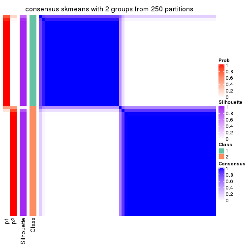
consensus_heatmap(res, k = 3)
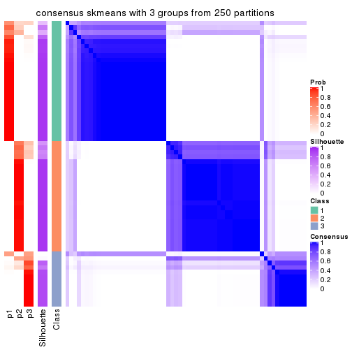
consensus_heatmap(res, k = 4)
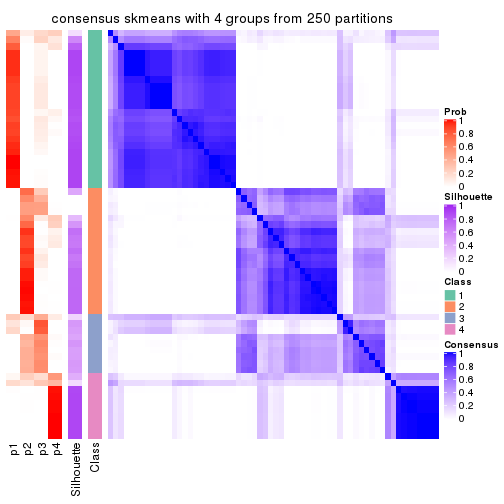
consensus_heatmap(res, k = 5)
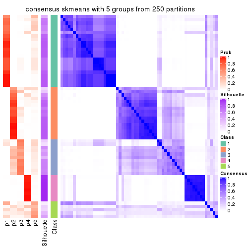
consensus_heatmap(res, k = 6)
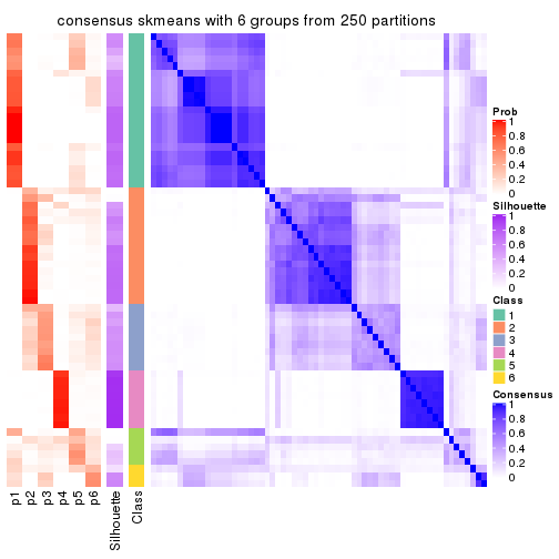
Heatmaps for the membership of samples in all partitions to see how consistent they are:
membership_heatmap(res, k = 2)
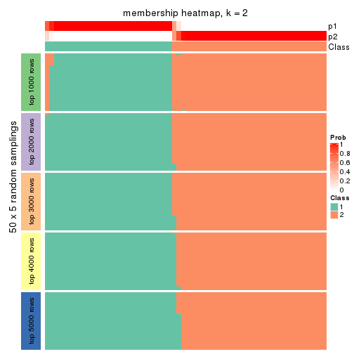
membership_heatmap(res, k = 3)
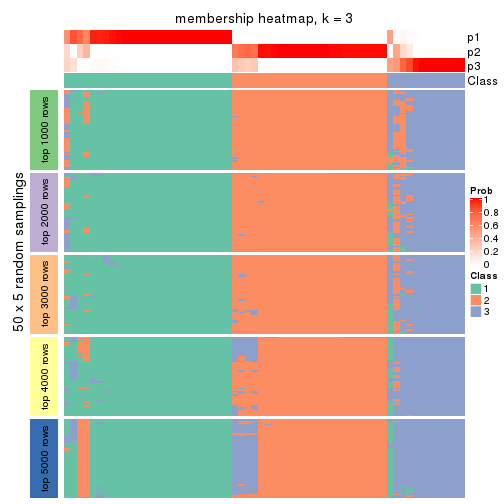
membership_heatmap(res, k = 4)
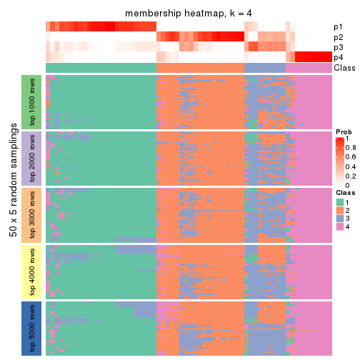
membership_heatmap(res, k = 5)
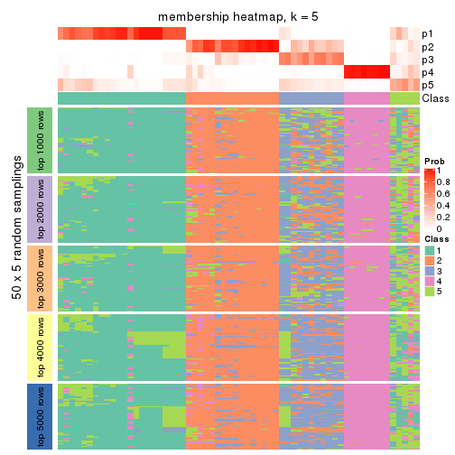
membership_heatmap(res, k = 6)
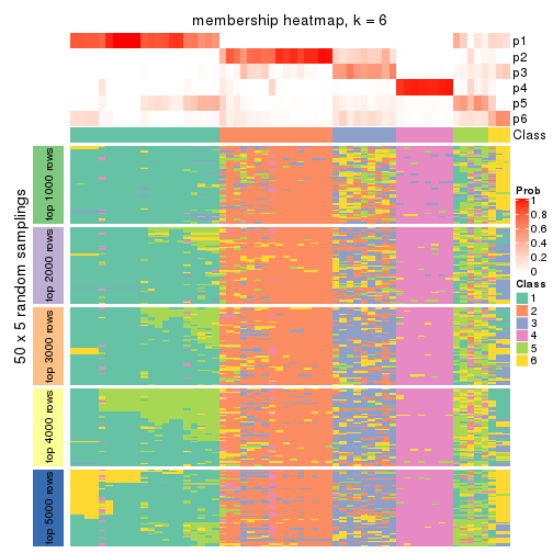
As soon as we have had the classes for columns, we can look for signatures which are significantly different between classes which can be candidate marks for certain classes. Following are the heatmaps for signatures.
Signature heatmaps where rows are scaled:
get_signatures(res, k = 2)
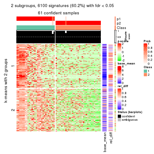
get_signatures(res, k = 3)
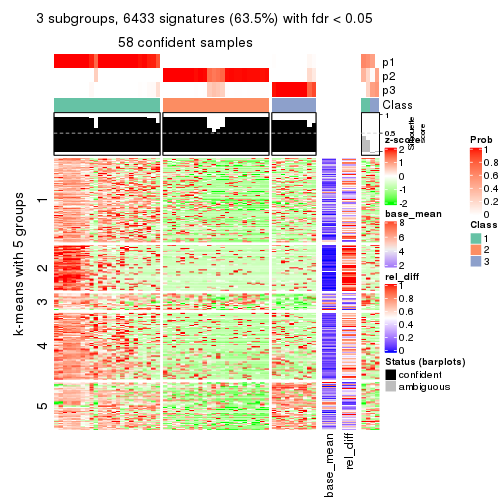
get_signatures(res, k = 4)
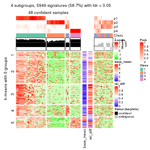
get_signatures(res, k = 5)
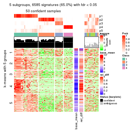
get_signatures(res, k = 6)
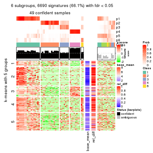
Signature heatmaps where rows are not scaled:
get_signatures(res, k = 2, scale_rows = FALSE)
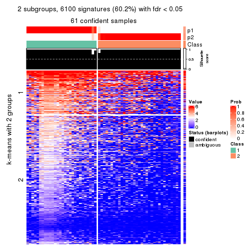
get_signatures(res, k = 3, scale_rows = FALSE)
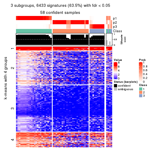
get_signatures(res, k = 4, scale_rows = FALSE)
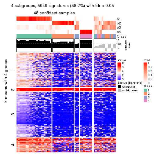
get_signatures(res, k = 5, scale_rows = FALSE)
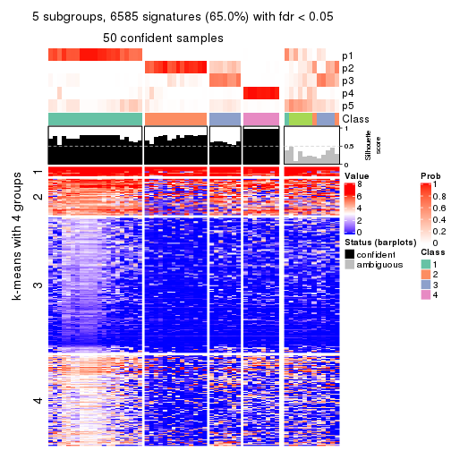
get_signatures(res, k = 6, scale_rows = FALSE)
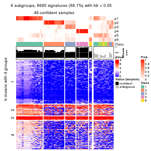
Compare the overlap of signatures from different k:
compare_signatures(res)
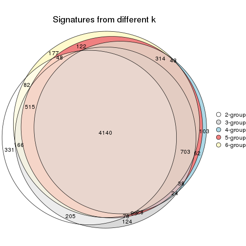
get_signature() returns a data frame invisibly. TO get the list of signatures, the function
call should be assigned to a variable explicitly. In following code, if plot argument is set
to FALSE, no heatmap is plotted while only the differential analysis is performed.
# code only for demonstration
tb = get_signature(res, k = ..., plot = FALSE)
An example of the output of tb is:
#>   which_row         fdr    mean_1    mean_2 scaled_mean_1 scaled_mean_2 km
#> 1        38 0.042760348  8.373488  9.131774    -0.5533452     0.5164555  1
#> 2        40 0.018707592  7.106213  8.469186    -0.6173731     0.5762149  1
#> 3        55 0.019134737 10.221463 11.207825    -0.6159697     0.5749050  1
#> 4        59 0.006059896  5.921854  7.869574    -0.6899429     0.6439467  1
#> 5        60 0.018055526  8.928898 10.211722    -0.6204761     0.5791110  1
#> 6        98 0.009384629 15.714769 14.887706     0.6635654    -0.6193277  2
...
The columns in tb are:
which_row: row indices corresponding to the input matrix.fdr: FDR for the differential test. mean_x: The mean value in group x.scaled_mean_x: The mean value in group x after rows are scaled.km: Row groups if k-means clustering is applied to rows.UMAP plot which shows how samples are separated.
dimension_reduction(res, k = 2, method = "UMAP")
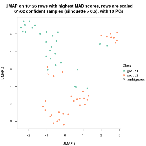
dimension_reduction(res, k = 3, method = "UMAP")
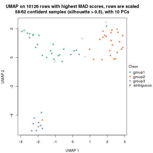
dimension_reduction(res, k = 4, method = "UMAP")
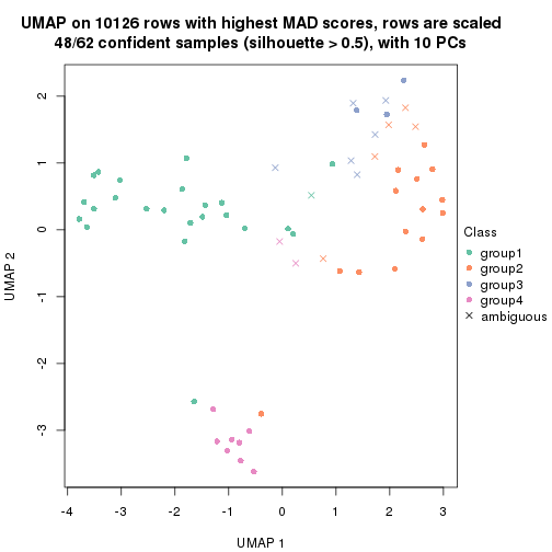
dimension_reduction(res, k = 5, method = "UMAP")
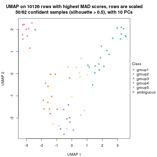
dimension_reduction(res, k = 6, method = "UMAP")
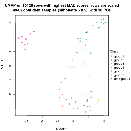
Following heatmap shows how subgroups are split when increasing k:
collect_classes(res)
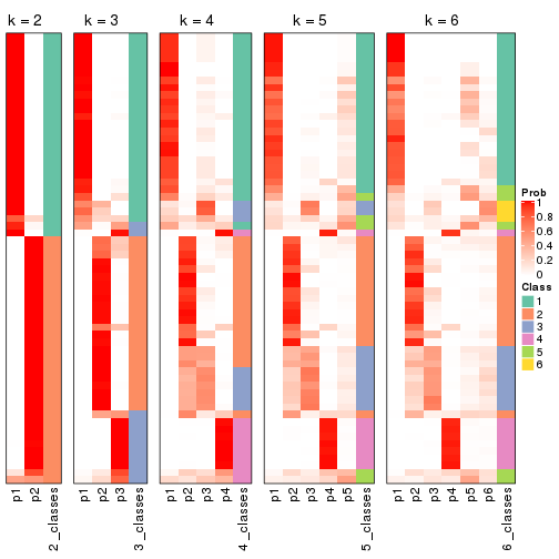
If matrix rows can be associated to genes, consider to use functional_enrichment(res,
...) to perform function enrichment for the signature genes. See this vignette for more detailed explanations.
The object with results only for a single top-value method and a single partition method can be extracted as:
res = res_list["MAD", "pam"]
# you can also extract it by
# res = res_list["MAD:pam"]
A summary of res and all the functions that can be applied to it:
res
#> A 'ConsensusPartition' object with k = 2, 3, 4, 5, 6.
#>   On a matrix with 10126 rows and 62 columns.
#>   Top rows (1000, 2000, 3000, 4000, 5000) are extracted by 'MAD' method.
#>   Subgroups are detected by 'pam' method.
#>   Performed in total 1250 partitions by row resampling.
#>   Best k for subgroups seems to be 3.
#>
#> Following methods can be applied to this 'ConsensusPartition' object:
#>  [1] "cola_report"             "collect_classes"         "collect_plots"
#>  [4] "collect_stats"           "colnames"                "compare_signatures"
#>  [7] "consensus_heatmap"       "dimension_reduction"     "functional_enrichment"
#> [10] "get_anno_col"            "get_anno"                "get_classes"
#> [13] "get_consensus"           "get_matrix"              "get_membership"
#> [16] "get_param"               "get_signatures"          "get_stats"
#> [19] "is_best_k"               "is_stable_k"             "membership_heatmap"
#> [22] "ncol"                    "nrow"                    "plot_ecdf"
#> [25] "rownames"                "select_partition_number" "show"
#> [28] "suggest_best_k"          "test_to_known_factors"
collect_plots() function collects all the plots made from res for all k (number of partitions)
into one single page to provide an easy and fast comparison between different k.
collect_plots(res)
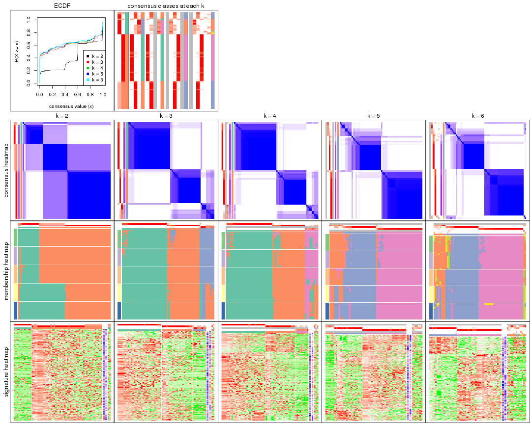
The plots are:
k and the heatmap of
predicted classes for each k.k.k.k.All the plots in panels can be made by individual functions and they are plotted later in this section.
select_partition_number() produces several plots showing different
statistics for choosing “optimized” k. There are following statistics:
k;k, the area increased is defined as \(A_k - A_{k-1}\).The detailed explanations of these statistics can be found in the cola vignette.
Generally speaking, lower PAC score, higher mean silhouette score or higher
concordance corresponds to better partition. Rand index and Jaccard index
measure how similar the current partition is compared to partition with k-1.
If they are too similar, we won't accept k is better than k-1.
select_partition_number(res)

The numeric values for all these statistics can be obtained by get_stats().
get_stats(res)
#>   k 1-PAC mean_silhouette concordance area_increased  Rand Jaccard
#> 2 2 0.563           0.728       0.872        0.40703 0.645   0.645
#> 3 3 0.766           0.874       0.935        0.47859 0.655   0.495
#> 4 4 0.770           0.841       0.909        0.02675 0.979   0.947
#> 5 5 0.751           0.828       0.898        0.00916 1.000   1.000
#> 6 6 0.722           0.723       0.893        0.01525 0.973   0.930
suggest_best_k() suggests the best \(k\) based on these statistics. The rules are as follows:
suggest_best_k(res)
#> [1] 3
Following shows the table of the partitions (You need to click the show/hide
code output link to see it). The membership matrix (columns with name p*)
is inferred by
clue::cl_consensus()
function with the SE method. Basically the value in the membership matrix
represents the probability to belong to a certain group. The finall class
label for an item is determined with the group with highest probability it
belongs to.
In get_classes() function, the entropy is calculated from the membership
matrix and the silhouette score is calculated from the consensus matrix.
cbind(get_classes(res, k = 2), get_membership(res, k = 2))
#>            class entropy silhouette    p1    p2
#> SRR764776      2  0.0000      0.812 0.000 1.000
#> SRR764777      2  0.0000      0.812 0.000 1.000
#> SRR764778      2  0.0000      0.812 0.000 1.000
#> SRR764779      2  0.0000      0.812 0.000 1.000
#> SRR764780      2  0.0000      0.812 0.000 1.000
#> SRR764781      2  0.0000      0.812 0.000 1.000
#> SRR764782      2  0.0000      0.812 0.000 1.000
#> SRR764783      2  0.0000      0.812 0.000 1.000
#> SRR764784      2  0.0000      0.812 0.000 1.000
#> SRR764785      1  0.9944     -0.133 0.544 0.456
#> SRR764786      1  0.9795      0.297 0.584 0.416
#> SRR764787      2  0.0000      0.812 0.000 1.000
#> SRR764788      2  0.0000      0.812 0.000 1.000
#> SRR764789      2  0.6148      0.726 0.152 0.848
#> SRR764790      1  0.0000      0.904 1.000 0.000
#> SRR764791      2  0.0000      0.812 0.000 1.000
#> SRR764792      2  0.0000      0.812 0.000 1.000
#> SRR764793      2  0.0000      0.812 0.000 1.000
#> SRR764794      2  0.0000      0.812 0.000 1.000
#> SRR764795      2  0.0000      0.812 0.000 1.000
#> SRR764796      2  0.0000      0.812 0.000 1.000
#> SRR764797      2  0.0000      0.812 0.000 1.000
#> SRR764798      2  0.9710      0.535 0.400 0.600
#> SRR764799      2  0.9710      0.535 0.400 0.600
#> SRR764800      2  0.0672      0.809 0.008 0.992
#> SRR764801      2  0.9710      0.535 0.400 0.600
#> SRR764802      2  0.0000      0.812 0.000 1.000
#> SRR764803      2  0.0000      0.812 0.000 1.000
#> SRR764804      1  0.0000      0.904 1.000 0.000
#> SRR764805      1  0.3733      0.832 0.928 0.072
#> SRR764806      2  0.9710      0.535 0.400 0.600
#> SRR764807      1  0.0000      0.904 1.000 0.000
#> SRR764808      1  0.0000      0.904 1.000 0.000
#> SRR764809      1  0.0938      0.897 0.988 0.012
#> SRR764810      1  0.1414      0.890 0.980 0.020
#> SRR764811      1  0.0000      0.904 1.000 0.000
#> SRR764812      1  0.0000      0.904 1.000 0.000
#> SRR764813      1  0.0000      0.904 1.000 0.000
#> SRR764814      2  0.9710      0.535 0.400 0.600
#> SRR764815      2  0.9710      0.535 0.400 0.600
#> SRR764816      2  0.9710      0.535 0.400 0.600
#> SRR764817      2  0.9710      0.535 0.400 0.600
#> SRR1066622     2  0.0000      0.812 0.000 1.000
#> SRR1066623     2  0.0000      0.812 0.000 1.000
#> SRR1066624     2  0.0000      0.812 0.000 1.000
#> SRR1066625     2  0.0000      0.812 0.000 1.000
#> SRR1066626     2  0.0000      0.812 0.000 1.000
#> SRR1066627     2  0.0000      0.812 0.000 1.000
#> SRR1066628     2  0.0000      0.812 0.000 1.000
#> SRR1066629     2  0.0000      0.812 0.000 1.000
#> SRR1066630     1  0.0000      0.904 1.000 0.000
#> SRR1066631     2  0.0000      0.812 0.000 1.000
#> SRR1066632     2  0.9710      0.535 0.400 0.600
#> SRR1066633     2  0.9710      0.535 0.400 0.600
#> SRR1066634     2  0.9710      0.535 0.400 0.600
#> SRR1066635     2  0.9710      0.535 0.400 0.600
#> SRR1066636     2  0.9710      0.535 0.400 0.600
#> SRR1066637     2  0.9710      0.535 0.400 0.600
#> SRR1066638     2  0.9710      0.535 0.400 0.600
#> SRR1066639     2  0.9710      0.535 0.400 0.600
#> SRR1066640     2  0.9710      0.535 0.400 0.600
#> SRR1066641     1  0.0000      0.904 1.000 0.000
cbind(get_classes(res, k = 3), get_membership(res, k = 3))
#>            class entropy silhouette    p1    p2    p3
#> SRR764776      1  0.0000      0.978 1.000 0.000 0.000
#> SRR764777      1  0.0000      0.978 1.000 0.000 0.000
#> SRR764778      1  0.0000      0.978 1.000 0.000 0.000
#> SRR764779      1  0.0000      0.978 1.000 0.000 0.000
#> SRR764780      1  0.0000      0.978 1.000 0.000 0.000
#> SRR764781      1  0.0000      0.978 1.000 0.000 0.000
#> SRR764782      1  0.0000      0.978 1.000 0.000 0.000
#> SRR764783      1  0.0000      0.978 1.000 0.000 0.000
#> SRR764784      1  0.0000      0.978 1.000 0.000 0.000
#> SRR764785      2  0.5067      0.760 0.052 0.832 0.116
#> SRR764786      3  0.6154      0.237 0.408 0.000 0.592
#> SRR764787      1  0.0000      0.978 1.000 0.000 0.000
#> SRR764788      1  0.0000      0.978 1.000 0.000 0.000
#> SRR764789      2  0.5098      0.498 0.248 0.752 0.000
#> SRR764790      3  0.0000      0.675 0.000 0.000 1.000
#> SRR764791      1  0.3412      0.856 0.876 0.124 0.000
#> SRR764792      1  0.3686      0.829 0.860 0.140 0.000
#> SRR764793      1  0.0000      0.978 1.000 0.000 0.000
#> SRR764794      1  0.3551      0.844 0.868 0.132 0.000
#> SRR764795      1  0.0000      0.978 1.000 0.000 0.000
#> SRR764796      1  0.0000      0.978 1.000 0.000 0.000
#> SRR764797      1  0.0000      0.978 1.000 0.000 0.000
#> SRR764798      2  0.0000      0.933 0.000 1.000 0.000
#> SRR764799      2  0.0000      0.933 0.000 1.000 0.000
#> SRR764800      1  0.0424      0.971 0.992 0.008 0.000
#> SRR764801      2  0.0000      0.933 0.000 1.000 0.000
#> SRR764802      1  0.0000      0.978 1.000 0.000 0.000
#> SRR764803      1  0.0000      0.978 1.000 0.000 0.000
#> SRR764804      3  0.5560      0.694 0.000 0.300 0.700
#> SRR764805      2  0.2356      0.863 0.000 0.928 0.072
#> SRR764806      2  0.0000      0.933 0.000 1.000 0.000
#> SRR764807      3  0.0000      0.675 0.000 0.000 1.000
#> SRR764808      3  0.0000      0.675 0.000 0.000 1.000
#> SRR764809      2  0.3482      0.793 0.000 0.872 0.128
#> SRR764810      2  0.3816      0.762 0.000 0.852 0.148
#> SRR764811      3  0.6126      0.611 0.000 0.400 0.600
#> SRR764812      3  0.5859      0.669 0.000 0.344 0.656
#> SRR764813      3  0.6168      0.590 0.000 0.412 0.588
#> SRR764814      2  0.3941      0.708 0.156 0.844 0.000
#> SRR764815      2  0.0000      0.933 0.000 1.000 0.000
#> SRR764816      2  0.0000      0.933 0.000 1.000 0.000
#> SRR764817      2  0.0000      0.933 0.000 1.000 0.000
#> SRR1066622     1  0.0000      0.978 1.000 0.000 0.000
#> SRR1066623     1  0.0000      0.978 1.000 0.000 0.000
#> SRR1066624     1  0.0237      0.975 0.996 0.004 0.000
#> SRR1066625     1  0.3482      0.851 0.872 0.128 0.000
#> SRR1066626     1  0.0237      0.975 0.996 0.004 0.000
#> SRR1066627     1  0.0000      0.978 1.000 0.000 0.000
#> SRR1066628     1  0.0747      0.966 0.984 0.016 0.000
#> SRR1066629     1  0.0000      0.978 1.000 0.000 0.000
#> SRR1066630     3  0.6140      0.605 0.000 0.404 0.596
#> SRR1066631     1  0.0237      0.975 0.996 0.004 0.000
#> SRR1066632     2  0.0000      0.933 0.000 1.000 0.000
#> SRR1066633     2  0.0000      0.933 0.000 1.000 0.000
#> SRR1066634     2  0.0000      0.933 0.000 1.000 0.000
#> SRR1066635     2  0.0000      0.933 0.000 1.000 0.000
#> SRR1066636     2  0.0000      0.933 0.000 1.000 0.000
#> SRR1066637     2  0.0000      0.933 0.000 1.000 0.000
#> SRR1066638     2  0.0000      0.933 0.000 1.000 0.000
#> SRR1066639     2  0.0000      0.933 0.000 1.000 0.000
#> SRR1066640     2  0.0000      0.933 0.000 1.000 0.000
#> SRR1066641     3  0.5431      0.697 0.000 0.284 0.716
cbind(get_classes(res, k = 4), get_membership(res, k = 4))
#>            class entropy silhouette    p1    p2 p3    p4
#> SRR764776      1  0.0000      0.959 1.000 0.000 NA 0.000
#> SRR764777      1  0.0000      0.959 1.000 0.000 NA 0.000
#> SRR764778      1  0.0000      0.959 1.000 0.000 NA 0.000
#> SRR764779      1  0.0000      0.959 1.000 0.000 NA 0.000
#> SRR764780      1  0.0000      0.959 1.000 0.000 NA 0.000
#> SRR764781      1  0.0000      0.959 1.000 0.000 NA 0.000
#> SRR764782      1  0.0000      0.959 1.000 0.000 NA 0.000
#> SRR764783      1  0.0000      0.959 1.000 0.000 NA 0.000
#> SRR764784      1  0.0000      0.959 1.000 0.000 NA 0.000
#> SRR764785      2  0.5017      0.734 0.052 0.808 NA 0.056
#> SRR764786      1  0.7684     -0.194 0.396 0.000 NA 0.388
#> SRR764787      1  0.0000      0.959 1.000 0.000 NA 0.000
#> SRR764788      1  0.0000      0.959 1.000 0.000 NA 0.000
#> SRR764789      2  0.4040      0.493 0.248 0.752 NA 0.000
#> SRR764790      4  0.4985      0.699 0.000 0.000 NA 0.532
#> SRR764791      1  0.2704      0.844 0.876 0.124 NA 0.000
#> SRR764792      1  0.2921      0.819 0.860 0.140 NA 0.000
#> SRR764793      1  0.0000      0.959 1.000 0.000 NA 0.000
#> SRR764794      1  0.2814      0.833 0.868 0.132 NA 0.000
#> SRR764795      1  0.0000      0.959 1.000 0.000 NA 0.000
#> SRR764796      1  0.0000      0.959 1.000 0.000 NA 0.000
#> SRR764797      1  0.0000      0.959 1.000 0.000 NA 0.000
#> SRR764798      2  0.0000      0.911 0.000 1.000 NA 0.000
#> SRR764799      2  0.0000      0.911 0.000 1.000 NA 0.000
#> SRR764800      1  0.0336      0.953 0.992 0.008 NA 0.000
#> SRR764801      2  0.0000      0.911 0.000 1.000 NA 0.000
#> SRR764802      1  0.0000      0.959 1.000 0.000 NA 0.000
#> SRR764803      1  0.0000      0.959 1.000 0.000 NA 0.000
#> SRR764804      4  0.6159      0.682 0.000 0.196 NA 0.672
#> SRR764805      2  0.4057      0.739 0.000 0.816 NA 0.032
#> SRR764806      2  0.0000      0.911 0.000 1.000 NA 0.000
#> SRR764807      4  0.4454      0.710 0.000 0.000 NA 0.692
#> SRR764808      4  0.4961      0.700 0.000 0.000 NA 0.552
#> SRR764809      2  0.4719      0.680 0.000 0.772 NA 0.048
#> SRR764810      2  0.6078      0.396 0.000 0.620 NA 0.068
#> SRR764811      4  0.5989      0.534 0.000 0.400 NA 0.556
#> SRR764812      4  0.6147      0.681 0.000 0.200 NA 0.672
#> SRR764813      4  0.5847      0.530 0.000 0.404 NA 0.560
#> SRR764814      2  0.3123      0.702 0.156 0.844 NA 0.000
#> SRR764815      2  0.0000      0.911 0.000 1.000 NA 0.000
#> SRR764816      2  0.0000      0.911 0.000 1.000 NA 0.000
#> SRR764817      2  0.0000      0.911 0.000 1.000 NA 0.000
#> SRR1066622     1  0.0000      0.959 1.000 0.000 NA 0.000
#> SRR1066623     1  0.0000      0.959 1.000 0.000 NA 0.000
#> SRR1066624     1  0.0188      0.957 0.996 0.004 NA 0.000
#> SRR1066625     1  0.2760      0.839 0.872 0.128 NA 0.000
#> SRR1066626     1  0.0188      0.957 0.996 0.004 NA 0.000
#> SRR1066627     1  0.0000      0.959 1.000 0.000 NA 0.000
#> SRR1066628     1  0.0592      0.948 0.984 0.016 NA 0.000
#> SRR1066629     1  0.0000      0.959 1.000 0.000 NA 0.000
#> SRR1066630     4  0.6332      0.525 0.000 0.404 NA 0.532
#> SRR1066631     1  0.0188      0.957 0.996 0.004 NA 0.000
#> SRR1066632     2  0.0000      0.911 0.000 1.000 NA 0.000
#> SRR1066633     2  0.0000      0.911 0.000 1.000 NA 0.000
#> SRR1066634     2  0.0000      0.911 0.000 1.000 NA 0.000
#> SRR1066635     2  0.0000      0.911 0.000 1.000 NA 0.000
#> SRR1066636     2  0.0000      0.911 0.000 1.000 NA 0.000
#> SRR1066637     2  0.0000      0.911 0.000 1.000 NA 0.000
#> SRR1066638     2  0.0000      0.911 0.000 1.000 NA 0.000
#> SRR1066639     2  0.0000      0.911 0.000 1.000 NA 0.000
#> SRR1066640     2  0.0000      0.911 0.000 1.000 NA 0.000
#> SRR1066641     4  0.2494      0.703 0.000 0.036 NA 0.916
cbind(get_classes(res, k = 5), get_membership(res, k = 5))
#>            class entropy silhouette p1    p2    p3    p4 p5
#> SRR764776      4  0.0000      0.957 NA 0.000 0.000 1.000 NA
#> SRR764777      4  0.0000      0.957 NA 0.000 0.000 1.000 NA
#> SRR764778      4  0.0000      0.957 NA 0.000 0.000 1.000 NA
#> SRR764779      4  0.0000      0.957 NA 0.000 0.000 1.000 NA
#> SRR764780      4  0.0000      0.957 NA 0.000 0.000 1.000 NA
#> SRR764781      4  0.0000      0.957 NA 0.000 0.000 1.000 NA
#> SRR764782      4  0.0000      0.957 NA 0.000 0.000 1.000 NA
#> SRR764783      4  0.0000      0.957 NA 0.000 0.000 1.000 NA
#> SRR764784      4  0.0000      0.957 NA 0.000 0.000 1.000 NA
#> SRR764785      3  0.4280      0.741 NA 0.052 0.824 0.052 NA
#> SRR764786      4  0.7087     -0.227 NA 0.368 0.000 0.384 NA
#> SRR764787      4  0.0000      0.957 NA 0.000 0.000 1.000 NA
#> SRR764788      4  0.0000      0.957 NA 0.000 0.000 1.000 NA
#> SRR764789      3  0.3480      0.489 NA 0.000 0.752 0.248 NA
#> SRR764790      2  0.4653      0.700 NA 0.516 0.000 0.000 NA
#> SRR764791      4  0.2329      0.843 NA 0.000 0.124 0.876 NA
#> SRR764792      4  0.2516      0.818 NA 0.000 0.140 0.860 NA
#> SRR764793      4  0.0000      0.957 NA 0.000 0.000 1.000 NA
#> SRR764794      4  0.2424      0.831 NA 0.000 0.132 0.868 NA
#> SRR764795      4  0.0000      0.957 NA 0.000 0.000 1.000 NA
#> SRR764796      4  0.0000      0.957 NA 0.000 0.000 1.000 NA
#> SRR764797      4  0.0000      0.957 NA 0.000 0.000 1.000 NA
#> SRR764798      3  0.0000      0.902 NA 0.000 1.000 0.000 NA
#> SRR764799      3  0.0000      0.902 NA 0.000 1.000 0.000 NA
#> SRR764800      4  0.0290      0.952 NA 0.000 0.008 0.992 NA
#> SRR764801      3  0.0000      0.902 NA 0.000 1.000 0.000 NA
#> SRR764802      4  0.0000      0.957 NA 0.000 0.000 1.000 NA
#> SRR764803      4  0.0000      0.957 NA 0.000 0.000 1.000 NA
#> SRR764804      2  0.6220      0.680 NA 0.524 0.168 0.000 NA
#> SRR764805      3  0.4172      0.729 NA 0.028 0.812 0.000 NA
#> SRR764806      3  0.0000      0.902 NA 0.000 1.000 0.000 NA
#> SRR764807      2  0.3977      0.704 NA 0.764 0.000 0.000 NA
#> SRR764808      2  0.4291      0.700 NA 0.536 0.000 0.000 NA
#> SRR764809      3  0.5852      0.369 NA 0.016 0.600 0.000 NA
#> SRR764810      3  0.5331      0.353 NA 0.048 0.600 0.000 NA
#> SRR764811      2  0.6638      0.474 NA 0.464 0.400 0.000 NA
#> SRR764812      2  0.6273      0.676 NA 0.524 0.184 0.000 NA
#> SRR764813      2  0.5857      0.492 NA 0.528 0.400 0.000 NA
#> SRR764814      3  0.2690      0.695 NA 0.000 0.844 0.156 NA
#> SRR764815      3  0.0000      0.902 NA 0.000 1.000 0.000 NA
#> SRR764816      3  0.0000      0.902 NA 0.000 1.000 0.000 NA
#> SRR764817      3  0.0000      0.902 NA 0.000 1.000 0.000 NA
#> SRR1066622     4  0.0290      0.954 NA 0.000 0.000 0.992 NA
#> SRR1066623     4  0.0290      0.954 NA 0.000 0.000 0.992 NA
#> SRR1066624     4  0.0162      0.955 NA 0.000 0.004 0.996 NA
#> SRR1066625     4  0.2377      0.837 NA 0.000 0.128 0.872 NA
#> SRR1066626     4  0.0451      0.953 NA 0.000 0.004 0.988 NA
#> SRR1066627     4  0.0000      0.957 NA 0.000 0.000 1.000 NA
#> SRR1066628     4  0.0798      0.945 NA 0.000 0.016 0.976 NA
#> SRR1066629     4  0.0290      0.954 NA 0.000 0.000 0.992 NA
#> SRR1066630     2  0.6004      0.494 NA 0.516 0.400 0.000 NA
#> SRR1066631     4  0.0451      0.953 NA 0.000 0.004 0.988 NA
#> SRR1066632     3  0.0000      0.902 NA 0.000 1.000 0.000 NA
#> SRR1066633     3  0.0000      0.902 NA 0.000 1.000 0.000 NA
#> SRR1066634     3  0.0000      0.902 NA 0.000 1.000 0.000 NA
#> SRR1066635     3  0.0000      0.902 NA 0.000 1.000 0.000 NA
#> SRR1066636     3  0.0000      0.902 NA 0.000 1.000 0.000 NA
#> SRR1066637     3  0.0000      0.902 NA 0.000 1.000 0.000 NA
#> SRR1066638     3  0.0000      0.902 NA 0.000 1.000 0.000 NA
#> SRR1066639     3  0.0000      0.902 NA 0.000 1.000 0.000 NA
#> SRR1066640     3  0.0000      0.902 NA 0.000 1.000 0.000 NA
#> SRR1066641     2  0.3579      0.674 NA 0.756 0.000 0.000 NA
cbind(get_classes(res, k = 6), get_membership(res, k = 6))
#>            class entropy silhouette p1    p2    p3    p4    p5    p6
#> SRR764776      4  0.0000     0.9717 NA 0.000 0.000 1.000 0.000 0.000
#> SRR764777      4  0.0000     0.9717 NA 0.000 0.000 1.000 0.000 0.000
#> SRR764778      4  0.0000     0.9717 NA 0.000 0.000 1.000 0.000 0.000
#> SRR764779      4  0.0000     0.9717 NA 0.000 0.000 1.000 0.000 0.000
#> SRR764780      4  0.0000     0.9717 NA 0.000 0.000 1.000 0.000 0.000
#> SRR764781      4  0.0000     0.9717 NA 0.000 0.000 1.000 0.000 0.000
#> SRR764782      4  0.0000     0.9717 NA 0.000 0.000 1.000 0.000 0.000
#> SRR764783      4  0.0000     0.9717 NA 0.000 0.000 1.000 0.000 0.000
#> SRR764784      4  0.0000     0.9717 NA 0.000 0.000 1.000 0.000 0.000
#> SRR764785      3  0.4435     0.7267 NA 0.036 0.808 0.052 0.032 0.040
#> SRR764786      2  0.7474    -0.1209 NA 0.396 0.000 0.348 0.036 0.116
#> SRR764787      4  0.0000     0.9717 NA 0.000 0.000 1.000 0.000 0.000
#> SRR764788      4  0.0000     0.9717 NA 0.000 0.000 1.000 0.000 0.000
#> SRR764789      3  0.3126     0.4901 NA 0.000 0.752 0.248 0.000 0.000
#> SRR764790      2  0.0603    -0.2502 NA 0.980 0.000 0.000 0.000 0.016
#> SRR764791      4  0.2092     0.8484 NA 0.000 0.124 0.876 0.000 0.000
#> SRR764792      4  0.2260     0.8221 NA 0.000 0.140 0.860 0.000 0.000
#> SRR764793      4  0.0000     0.9717 NA 0.000 0.000 1.000 0.000 0.000
#> SRR764794      4  0.2178     0.8365 NA 0.000 0.132 0.868 0.000 0.000
#> SRR764795      4  0.0000     0.9717 NA 0.000 0.000 1.000 0.000 0.000
#> SRR764796      4  0.0000     0.9717 NA 0.000 0.000 1.000 0.000 0.000
#> SRR764797      4  0.0000     0.9717 NA 0.000 0.000 1.000 0.000 0.000
#> SRR764798      3  0.0000     0.8966 NA 0.000 1.000 0.000 0.000 0.000
#> SRR764799      3  0.0000     0.8966 NA 0.000 1.000 0.000 0.000 0.000
#> SRR764800      4  0.0260     0.9667 NA 0.000 0.008 0.992 0.000 0.000
#> SRR764801      3  0.0000     0.8966 NA 0.000 1.000 0.000 0.000 0.000
#> SRR764802      4  0.0000     0.9717 NA 0.000 0.000 1.000 0.000 0.000
#> SRR764803      4  0.0000     0.9717 NA 0.000 0.000 1.000 0.000 0.000
#> SRR764804      6  0.4609     0.0000 NA 0.420 0.040 0.000 0.000 0.540
#> SRR764805      3  0.4991     0.5033 NA 0.012 0.648 0.000 0.044 0.280
#> SRR764806      3  0.0000     0.8966 NA 0.000 1.000 0.000 0.000 0.000
#> SRR764807      2  0.4351    -0.3461 NA 0.720 0.000 0.000 0.000 0.108
#> SRR764808      2  0.0000    -0.2536 NA 1.000 0.000 0.000 0.000 0.000
#> SRR764809      3  0.4774     0.4126 NA 0.004 0.600 0.000 0.004 0.044
#> SRR764810      3  0.5161     0.4058 NA 0.020 0.600 0.000 0.316 0.064
#> SRR764811      2  0.6850    -0.0308 NA 0.400 0.256 0.000 0.004 0.040
#> SRR764812      2  0.5799    -0.4824 NA 0.428 0.180 0.000 0.000 0.392
#> SRR764813      2  0.6352     0.0830 NA 0.436 0.380 0.000 0.004 0.152
#> SRR764814      3  0.2416     0.6972 NA 0.000 0.844 0.156 0.000 0.000
#> SRR764815      3  0.0000     0.8966 NA 0.000 1.000 0.000 0.000 0.000
#> SRR764816      3  0.0000     0.8966 NA 0.000 1.000 0.000 0.000 0.000
#> SRR764817      3  0.0000     0.8966 NA 0.000 1.000 0.000 0.000 0.000
#> SRR1066622     4  0.0632     0.9601 NA 0.000 0.000 0.976 0.000 0.000
#> SRR1066623     4  0.0632     0.9601 NA 0.000 0.000 0.976 0.000 0.000
#> SRR1066624     4  0.0146     0.9697 NA 0.000 0.004 0.996 0.000 0.000
#> SRR1066625     4  0.2135     0.8428 NA 0.000 0.128 0.872 0.000 0.000
#> SRR1066626     4  0.0777     0.9591 NA 0.000 0.004 0.972 0.000 0.000
#> SRR1066627     4  0.0000     0.9717 NA 0.000 0.000 1.000 0.000 0.000
#> SRR1066628     4  0.1088     0.9520 NA 0.000 0.016 0.960 0.000 0.000
#> SRR1066629     4  0.0632     0.9601 NA 0.000 0.000 0.976 0.000 0.000
#> SRR1066630     2  0.6221     0.1033 NA 0.524 0.344 0.000 0.044 0.032
#> SRR1066631     4  0.0777     0.9589 NA 0.000 0.004 0.972 0.000 0.000
#> SRR1066632     3  0.0000     0.8966 NA 0.000 1.000 0.000 0.000 0.000
#> SRR1066633     3  0.0000     0.8966 NA 0.000 1.000 0.000 0.000 0.000
#> SRR1066634     3  0.0000     0.8966 NA 0.000 1.000 0.000 0.000 0.000
#> SRR1066635     3  0.0000     0.8966 NA 0.000 1.000 0.000 0.000 0.000
#> SRR1066636     3  0.0000     0.8966 NA 0.000 1.000 0.000 0.000 0.000
#> SRR1066637     3  0.0000     0.8966 NA 0.000 1.000 0.000 0.000 0.000
#> SRR1066638     3  0.0000     0.8966 NA 0.000 1.000 0.000 0.000 0.000
#> SRR1066639     3  0.0000     0.8966 NA 0.000 1.000 0.000 0.000 0.000
#> SRR1066640     3  0.0000     0.8966 NA 0.000 1.000 0.000 0.000 0.000
#> SRR1066641     5  0.4504     0.0000 NA 0.432 0.000 0.000 0.536 0.032
Heatmaps for the consensus matrix. It visualizes the probability of two samples to be in a same group.
consensus_heatmap(res, k = 2)
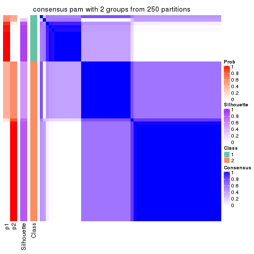
consensus_heatmap(res, k = 3)
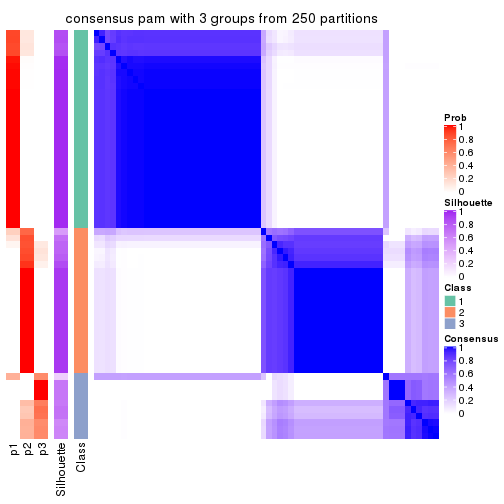
consensus_heatmap(res, k = 4)
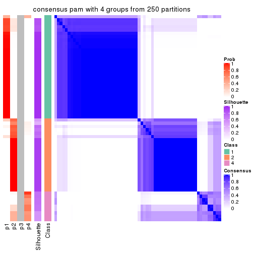
consensus_heatmap(res, k = 5)
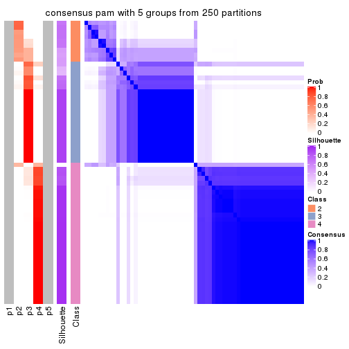
consensus_heatmap(res, k = 6)
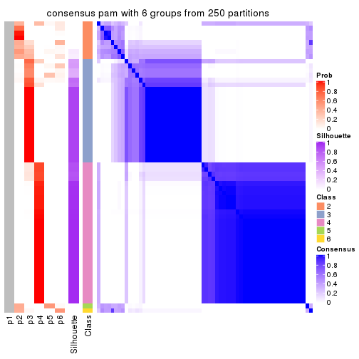
Heatmaps for the membership of samples in all partitions to see how consistent they are:
membership_heatmap(res, k = 2)
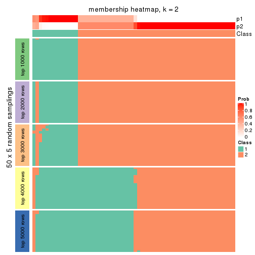
membership_heatmap(res, k = 3)
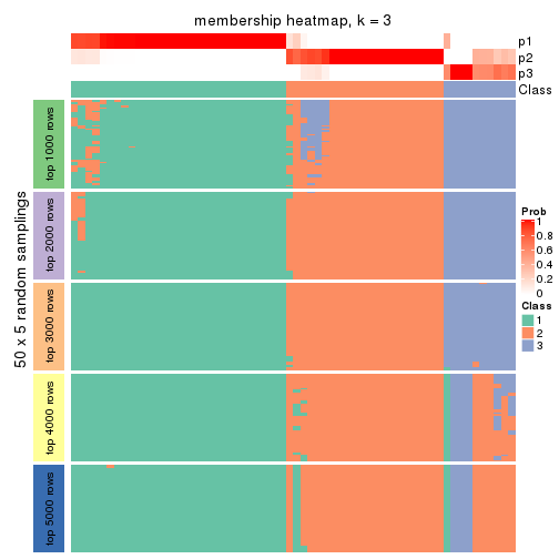
membership_heatmap(res, k = 4)
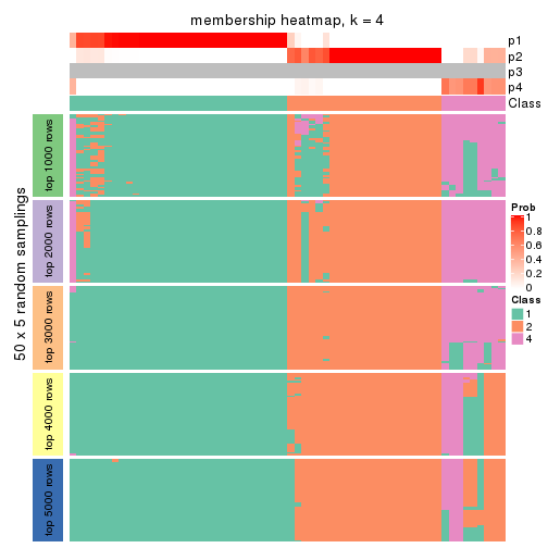
membership_heatmap(res, k = 5)
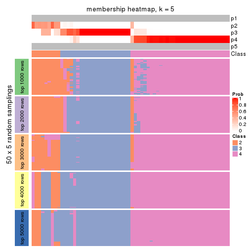
membership_heatmap(res, k = 6)
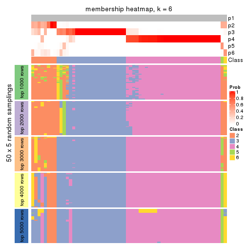
As soon as we have had the classes for columns, we can look for signatures which are significantly different between classes which can be candidate marks for certain classes. Following are the heatmaps for signatures.
Signature heatmaps where rows are scaled:
get_signatures(res, k = 2)
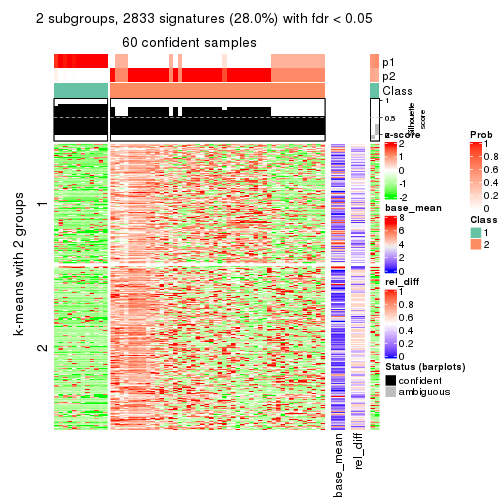
get_signatures(res, k = 3)
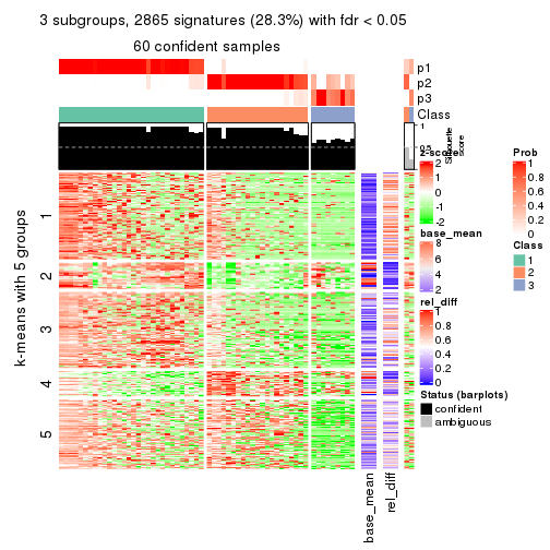
get_signatures(res, k = 4)
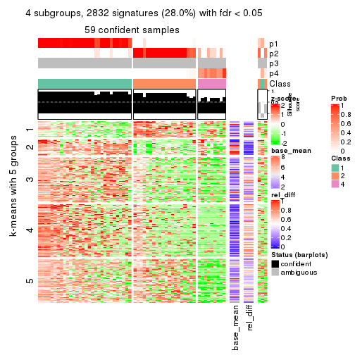
get_signatures(res, k = 5)
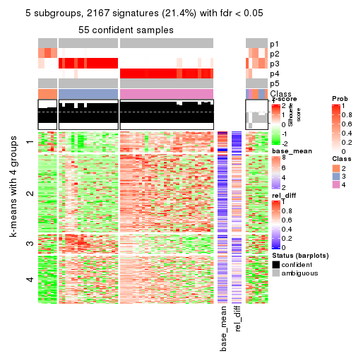
get_signatures(res, k = 6)
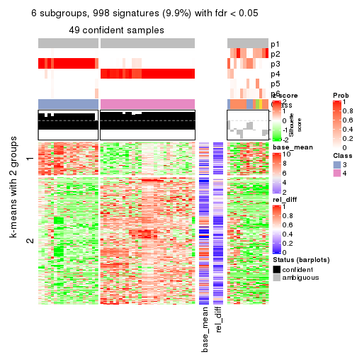
Signature heatmaps where rows are not scaled:
get_signatures(res, k = 2, scale_rows = FALSE)
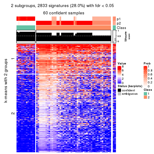
get_signatures(res, k = 3, scale_rows = FALSE)
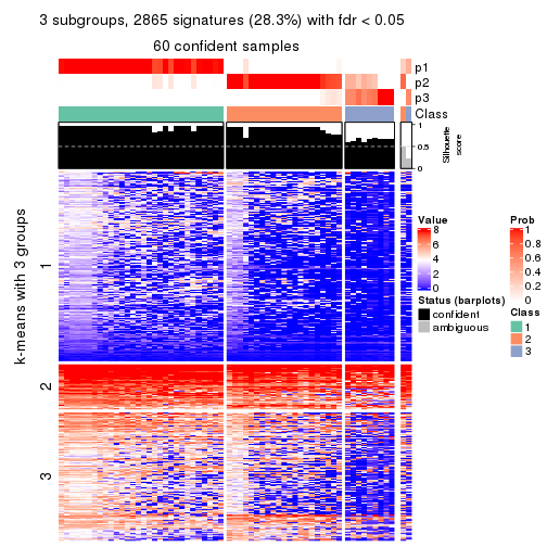
get_signatures(res, k = 4, scale_rows = FALSE)
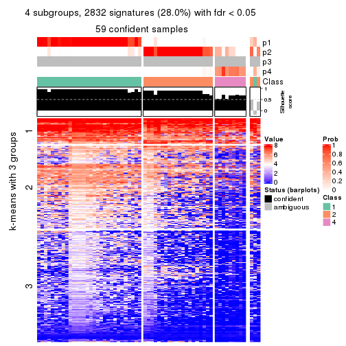
get_signatures(res, k = 5, scale_rows = FALSE)
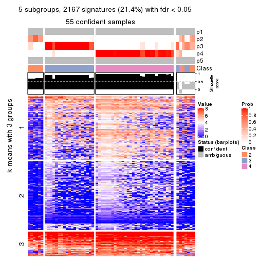
get_signatures(res, k = 6, scale_rows = FALSE)
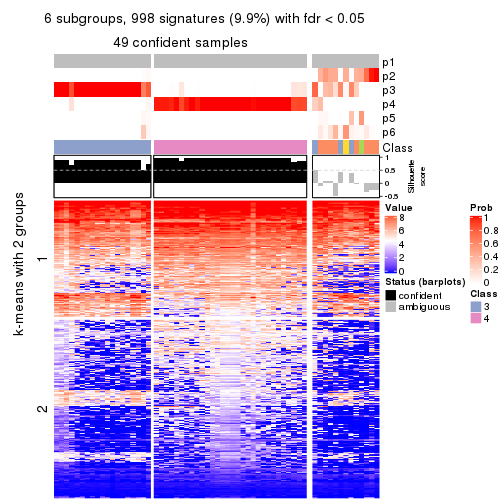
Compare the overlap of signatures from different k:
compare_signatures(res)
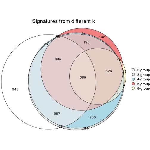
get_signature() returns a data frame invisibly. TO get the list of signatures, the function
call should be assigned to a variable explicitly. In following code, if plot argument is set
to FALSE, no heatmap is plotted while only the differential analysis is performed.
# code only for demonstration
tb = get_signature(res, k = ..., plot = FALSE)
An example of the output of tb is:
#>   which_row         fdr    mean_1    mean_2 scaled_mean_1 scaled_mean_2 km
#> 1        38 0.042760348  8.373488  9.131774    -0.5533452     0.5164555  1
#> 2        40 0.018707592  7.106213  8.469186    -0.6173731     0.5762149  1
#> 3        55 0.019134737 10.221463 11.207825    -0.6159697     0.5749050  1
#> 4        59 0.006059896  5.921854  7.869574    -0.6899429     0.6439467  1
#> 5        60 0.018055526  8.928898 10.211722    -0.6204761     0.5791110  1
#> 6        98 0.009384629 15.714769 14.887706     0.6635654    -0.6193277  2
...
The columns in tb are:
which_row: row indices corresponding to the input matrix.fdr: FDR for the differential test. mean_x: The mean value in group x.scaled_mean_x: The mean value in group x after rows are scaled.km: Row groups if k-means clustering is applied to rows.UMAP plot which shows how samples are separated.
dimension_reduction(res, k = 2, method = "UMAP")
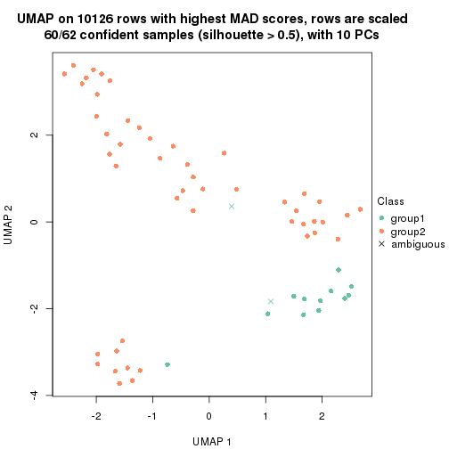
dimension_reduction(res, k = 3, method = "UMAP")
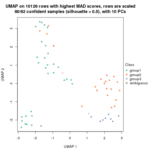
dimension_reduction(res, k = 4, method = "UMAP")
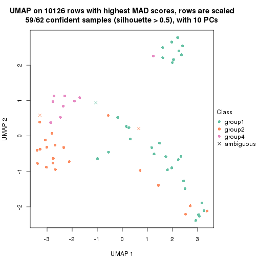
dimension_reduction(res, k = 5, method = "UMAP")
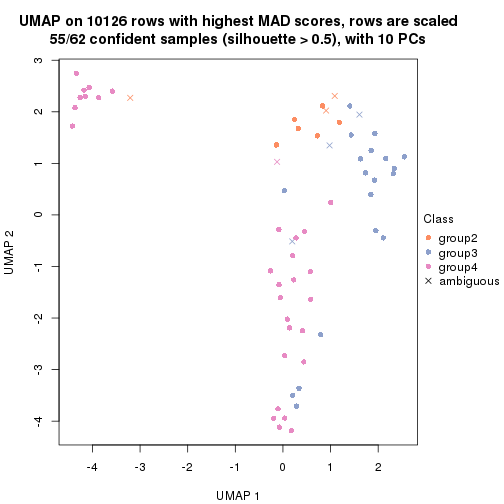
dimension_reduction(res, k = 6, method = "UMAP")
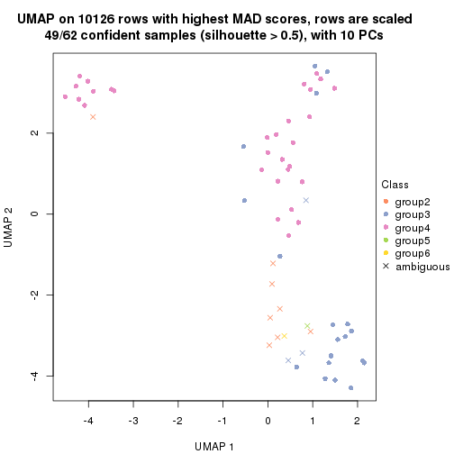
Following heatmap shows how subgroups are split when increasing k:
collect_classes(res)
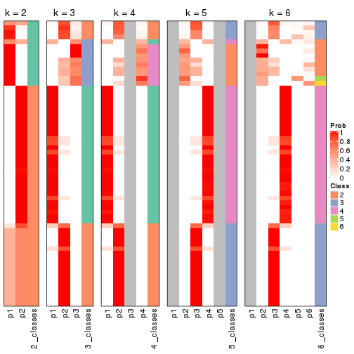
If matrix rows can be associated to genes, consider to use functional_enrichment(res,
...) to perform function enrichment for the signature genes. See this vignette for more detailed explanations.
The object with results only for a single top-value method and a single partition method can be extracted as:
res = res_list["MAD", "mclust"]
# you can also extract it by
# res = res_list["MAD:mclust"]
A summary of res and all the functions that can be applied to it:
res
#> A 'ConsensusPartition' object with k = 2, 3, 4, 5, 6.
#>   On a matrix with 10126 rows and 62 columns.
#>   Top rows (1000, 2000, 3000, 4000, 5000) are extracted by 'MAD' method.
#>   Subgroups are detected by 'mclust' method.
#>   Performed in total 1250 partitions by row resampling.
#>   Best k for subgroups seems to be 3.
#>
#> Following methods can be applied to this 'ConsensusPartition' object:
#>  [1] "cola_report"             "collect_classes"         "collect_plots"
#>  [4] "collect_stats"           "colnames"                "compare_signatures"
#>  [7] "consensus_heatmap"       "dimension_reduction"     "functional_enrichment"
#> [10] "get_anno_col"            "get_anno"                "get_classes"
#> [13] "get_consensus"           "get_matrix"              "get_membership"
#> [16] "get_param"               "get_signatures"          "get_stats"
#> [19] "is_best_k"               "is_stable_k"             "membership_heatmap"
#> [22] "ncol"                    "nrow"                    "plot_ecdf"
#> [25] "rownames"                "select_partition_number" "show"
#> [28] "suggest_best_k"          "test_to_known_factors"
collect_plots() function collects all the plots made from res for all k (number of partitions)
into one single page to provide an easy and fast comparison between different k.
collect_plots(res)
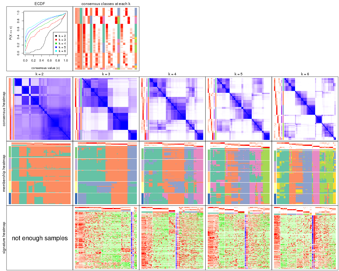
The plots are:
k and the heatmap of
predicted classes for each k.k.k.k.All the plots in panels can be made by individual functions and they are plotted later in this section.
select_partition_number() produces several plots showing different
statistics for choosing “optimized” k. There are following statistics:
k;k, the area increased is defined as \(A_k - A_{k-1}\).The detailed explanations of these statistics can be found in the cola vignette.
Generally speaking, lower PAC score, higher mean silhouette score or higher
concordance corresponds to better partition. Rand index and Jaccard index
measure how similar the current partition is compared to partition with k-1.
If they are too similar, we won't accept k is better than k-1.
select_partition_number(res)
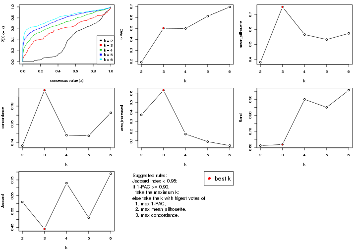
The numeric values for all these statistics can be obtained by get_stats().
get_stats(res)
#>   k 1-PAC mean_silhouette concordance area_increased  Rand Jaccard
#> 2 2 0.192           0.381       0.736         0.3718 0.611   0.611
#> 3 3 0.501           0.750       0.797         0.6298 0.618   0.440
#> 4 4 0.499           0.566       0.748         0.1703 0.900   0.730
#> 5 5 0.611           0.532       0.747         0.0906 0.850   0.511
#> 6 6 0.695           0.573       0.773         0.0492 0.957   0.790
suggest_best_k() suggests the best \(k\) based on these statistics. The rules are as follows:
suggest_best_k(res)
#> [1] 3
Following shows the table of the partitions (You need to click the show/hide
code output link to see it). The membership matrix (columns with name p*)
is inferred by
clue::cl_consensus()
function with the SE method. Basically the value in the membership matrix
represents the probability to belong to a certain group. The finall class
label for an item is determined with the group with highest probability it
belongs to.
In get_classes() function, the entropy is calculated from the membership
matrix and the silhouette score is calculated from the consensus matrix.
cbind(get_classes(res, k = 2), get_membership(res, k = 2))
#>            class entropy silhouette    p1    p2
#> SRR764776      2   0.278     0.6189 0.048 0.952
#> SRR764777      2   0.278     0.6189 0.048 0.952
#> SRR764778      2   0.278     0.6189 0.048 0.952
#> SRR764779      2   0.278     0.6189 0.048 0.952
#> SRR764780      2   0.278     0.6189 0.048 0.952
#> SRR764781      2   0.260     0.6212 0.044 0.956
#> SRR764782      2   0.343     0.6400 0.064 0.936
#> SRR764783      2   0.242     0.6363 0.040 0.960
#> SRR764784      2   0.388     0.6284 0.076 0.924
#> SRR764785      2   0.775     0.5326 0.228 0.772
#> SRR764786      2   0.706     0.5357 0.192 0.808
#> SRR764787      2   0.482     0.6178 0.104 0.896
#> SRR764788      2   0.327     0.6372 0.060 0.940
#> SRR764789      2   0.402     0.6381 0.080 0.920
#> SRR764790      2   0.983     0.2206 0.424 0.576
#> SRR764791      2   0.373     0.6387 0.072 0.928
#> SRR764792      2   0.456     0.6298 0.096 0.904
#> SRR764793      2   0.295     0.6418 0.052 0.948
#> SRR764794      2   0.680     0.5607 0.180 0.820
#> SRR764795      2   0.482     0.5945 0.104 0.896
#> SRR764796      2   0.671     0.5171 0.176 0.824
#> SRR764797      2   0.278     0.6432 0.048 0.952
#> SRR764798      2   0.634     0.5483 0.160 0.840
#> SRR764799      2   0.311     0.6377 0.056 0.944
#> SRR764800      2   0.260     0.6212 0.044 0.956
#> SRR764801      2   0.634     0.5483 0.160 0.840
#> SRR764802      2   0.260     0.6217 0.044 0.956
#> SRR764803      2   0.295     0.6165 0.052 0.948
#> SRR764804      2   0.995     0.0388 0.460 0.540
#> SRR764805      2   0.996     0.0264 0.464 0.536
#> SRR764806      2   1.000    -0.0559 0.488 0.512
#> SRR764807      2   0.904     0.3785 0.320 0.680
#> SRR764808      2   0.991     0.1814 0.444 0.556
#> SRR764809      2   0.996     0.0264 0.464 0.536
#> SRR764810      2   0.994     0.0499 0.456 0.544
#> SRR764811      2   0.994     0.0499 0.456 0.544
#> SRR764812      2   0.993     0.0597 0.452 0.548
#> SRR764813      2   0.855     0.4116 0.280 0.720
#> SRR764814      2   0.242     0.6403 0.040 0.960
#> SRR764815      2   0.358     0.6381 0.068 0.932
#> SRR764816      2   0.204     0.6414 0.032 0.968
#> SRR764817      2   0.242     0.6415 0.040 0.960
#> SRR1066622     1   0.995     0.2881 0.540 0.460
#> SRR1066623     1   0.994     0.2936 0.544 0.456
#> SRR1066624     2   0.993    -0.1874 0.452 0.548
#> SRR1066625     2   1.000    -0.2657 0.488 0.512
#> SRR1066626     1   0.994     0.2936 0.544 0.456
#> SRR1066627     1   0.995     0.2897 0.540 0.460
#> SRR1066628     1   0.994     0.2936 0.544 0.456
#> SRR1066629     1   0.994     0.2936 0.544 0.456
#> SRR1066630     1   0.990     0.2128 0.560 0.440
#> SRR1066631     1   0.994     0.2936 0.544 0.456
#> SRR1066632     1   0.992     0.1718 0.552 0.448
#> SRR1066633     2   0.990     0.0877 0.440 0.560
#> SRR1066634     1   0.991     0.1652 0.556 0.444
#> SRR1066635     1   0.998     0.1095 0.528 0.472
#> SRR1066636     1   0.992     0.1717 0.552 0.448
#> SRR1066637     1   0.991     0.1773 0.556 0.444
#> SRR1066638     1   0.991     0.1773 0.556 0.444
#> SRR1066639     1   0.991     0.1773 0.556 0.444
#> SRR1066640     1   0.992     0.1717 0.552 0.448
#> SRR1066641     2   0.995     0.0388 0.460 0.540
cbind(get_classes(res, k = 3), get_membership(res, k = 3))
#>            class entropy silhouette    p1    p2    p3
#> SRR764776      1  0.0237      0.753 0.996 0.004 0.000
#> SRR764777      1  0.0237      0.753 0.996 0.004 0.000
#> SRR764778      1  0.0237      0.753 0.996 0.004 0.000
#> SRR764779      1  0.0237      0.753 0.996 0.004 0.000
#> SRR764780      1  0.0424      0.754 0.992 0.008 0.000
#> SRR764781      1  0.0848      0.750 0.984 0.008 0.008
#> SRR764782      1  0.6141      0.659 0.736 0.032 0.232
#> SRR764783      1  0.0892      0.756 0.980 0.020 0.000
#> SRR764784      1  0.5858      0.650 0.740 0.020 0.240
#> SRR764785      1  0.6394      0.666 0.768 0.116 0.116
#> SRR764786      1  0.8141      0.434 0.624 0.260 0.116
#> SRR764787      1  0.7383      0.654 0.680 0.084 0.236
#> SRR764788      1  0.6276      0.666 0.736 0.040 0.224
#> SRR764789      1  0.5740      0.702 0.804 0.100 0.096
#> SRR764790      2  0.8933      0.428 0.276 0.556 0.168
#> SRR764791      1  0.7419      0.655 0.680 0.088 0.232
#> SRR764792      1  0.7745      0.670 0.648 0.092 0.260
#> SRR764793      1  0.6253      0.659 0.732 0.036 0.232
#> SRR764794      1  0.6031      0.695 0.788 0.096 0.116
#> SRR764795      1  0.6016      0.640 0.724 0.020 0.256
#> SRR764796      1  0.7061      0.554 0.632 0.036 0.332
#> SRR764797      1  0.1860      0.750 0.948 0.052 0.000
#> SRR764798      2  0.8196      0.507 0.284 0.608 0.108
#> SRR764799      1  0.5117      0.717 0.832 0.060 0.108
#> SRR764800      1  0.0747      0.755 0.984 0.016 0.000
#> SRR764801      2  0.8196      0.507 0.284 0.608 0.108
#> SRR764802      1  0.1015      0.747 0.980 0.008 0.012
#> SRR764803      1  0.1015      0.751 0.980 0.012 0.008
#> SRR764804      2  0.1289      0.849 0.032 0.968 0.000
#> SRR764805      2  0.0000      0.850 0.000 1.000 0.000
#> SRR764806      2  0.0000      0.850 0.000 1.000 0.000
#> SRR764807      2  0.8075      0.524 0.276 0.620 0.104
#> SRR764808      2  0.8599      0.477 0.276 0.584 0.140
#> SRR764809      2  0.0000      0.850 0.000 1.000 0.000
#> SRR764810      2  0.1289      0.849 0.032 0.968 0.000
#> SRR764811      2  0.2414      0.841 0.040 0.940 0.020
#> SRR764812      2  0.2443      0.841 0.032 0.940 0.028
#> SRR764813      2  0.8045      0.527 0.272 0.624 0.104
#> SRR764814      1  0.5117      0.719 0.832 0.060 0.108
#> SRR764815      1  0.6039      0.689 0.788 0.104 0.108
#> SRR764816      1  0.5117      0.717 0.832 0.060 0.108
#> SRR764817      1  0.5117      0.717 0.832 0.060 0.108
#> SRR1066622     3  0.6252      0.930 0.344 0.008 0.648
#> SRR1066623     3  0.5859      0.935 0.344 0.000 0.656
#> SRR1066624     3  0.7558      0.846 0.400 0.044 0.556
#> SRR1066625     3  0.7464      0.850 0.400 0.040 0.560
#> SRR1066626     3  0.5859      0.935 0.344 0.000 0.656
#> SRR1066627     3  0.5859      0.935 0.344 0.000 0.656
#> SRR1066628     3  0.5859      0.935 0.344 0.000 0.656
#> SRR1066629     3  0.5859      0.935 0.344 0.000 0.656
#> SRR1066630     3  0.7097      0.724 0.280 0.052 0.668
#> SRR1066631     3  0.5859      0.935 0.344 0.000 0.656
#> SRR1066632     2  0.0747      0.849 0.016 0.984 0.000
#> SRR1066633     2  0.2446      0.837 0.052 0.936 0.012
#> SRR1066634     2  0.1411      0.835 0.036 0.964 0.000
#> SRR1066635     2  0.0000      0.850 0.000 1.000 0.000
#> SRR1066636     2  0.0000      0.850 0.000 1.000 0.000
#> SRR1066637     2  0.0000      0.850 0.000 1.000 0.000
#> SRR1066638     2  0.0237      0.850 0.004 0.996 0.000
#> SRR1066639     2  0.0000      0.850 0.000 1.000 0.000
#> SRR1066640     2  0.0000      0.850 0.000 1.000 0.000
#> SRR1066641     2  0.1289      0.849 0.032 0.968 0.000
cbind(get_classes(res, k = 4), get_membership(res, k = 4))
#>            class entropy silhouette    p1    p2    p3    p4
#> SRR764776      1  0.0000      0.656 1.000 0.000 0.000 0.000
#> SRR764777      1  0.0000      0.656 1.000 0.000 0.000 0.000
#> SRR764778      1  0.0000      0.656 1.000 0.000 0.000 0.000
#> SRR764779      1  0.0000      0.656 1.000 0.000 0.000 0.000
#> SRR764780      1  0.2401      0.646 0.904 0.000 0.092 0.004
#> SRR764781      1  0.3448      0.623 0.828 0.000 0.168 0.004
#> SRR764782      3  0.5335     -0.114 0.488 0.004 0.504 0.004
#> SRR764783      1  0.5284      0.495 0.696 0.000 0.264 0.040
#> SRR764784      1  0.5039      0.264 0.592 0.000 0.404 0.004
#> SRR764785      3  0.7281      0.392 0.216 0.048 0.628 0.108
#> SRR764786      3  0.7888      0.331 0.192 0.096 0.600 0.112
#> SRR764787      3  0.4607      0.443 0.204 0.024 0.768 0.004
#> SRR764788      3  0.5233      0.135 0.412 0.004 0.580 0.004
#> SRR764789      1  0.7403     -0.112 0.480 0.028 0.408 0.084
#> SRR764790      2  0.9224      0.422 0.128 0.408 0.312 0.152
#> SRR764791      3  0.5202      0.350 0.312 0.016 0.668 0.004
#> SRR764792      3  0.4706      0.444 0.248 0.020 0.732 0.000
#> SRR764793      3  0.5269      0.081 0.428 0.004 0.564 0.004
#> SRR764794      3  0.7245      0.391 0.288 0.024 0.580 0.108
#> SRR764795      1  0.4950      0.310 0.620 0.000 0.376 0.004
#> SRR764796      1  0.6372      0.184 0.540 0.008 0.404 0.048
#> SRR764797      1  0.4713      0.493 0.700 0.004 0.292 0.004
#> SRR764798      2  0.7930      0.437 0.296 0.540 0.100 0.064
#> SRR764799      1  0.6208      0.457 0.736 0.088 0.112 0.064
#> SRR764800      1  0.1707      0.639 0.952 0.020 0.024 0.004
#> SRR764801      2  0.7930      0.437 0.296 0.540 0.100 0.064
#> SRR764802      1  0.3494      0.619 0.824 0.000 0.172 0.004
#> SRR764803      1  0.3539      0.616 0.820 0.000 0.176 0.004
#> SRR764804      2  0.4186      0.775 0.024 0.808 0.164 0.004
#> SRR764805      2  0.3355      0.779 0.000 0.836 0.160 0.004
#> SRR764806      2  0.0469      0.778 0.000 0.988 0.012 0.000
#> SRR764807      2  0.9080      0.460 0.156 0.432 0.300 0.112
#> SRR764808      2  0.9224      0.434 0.128 0.408 0.312 0.152
#> SRR764809      2  0.3306      0.779 0.000 0.840 0.156 0.004
#> SRR764810      2  0.4559      0.771 0.040 0.792 0.164 0.004
#> SRR764811      2  0.5467      0.741 0.056 0.716 0.224 0.004
#> SRR764812      2  0.5552      0.731 0.052 0.700 0.244 0.004
#> SRR764813      2  0.8964      0.478 0.156 0.452 0.288 0.104
#> SRR764814      1  0.4599      0.545 0.800 0.088 0.112 0.000
#> SRR764815      3  0.8352      0.271 0.384 0.124 0.432 0.060
#> SRR764816      1  0.5049      0.533 0.788 0.088 0.112 0.012
#> SRR764817      1  0.4599      0.545 0.800 0.088 0.112 0.000
#> SRR1066622     4  0.0524      0.830 0.008 0.000 0.004 0.988
#> SRR1066623     4  0.0000      0.830 0.000 0.000 0.000 1.000
#> SRR1066624     4  0.7553      0.376 0.248 0.032 0.140 0.580
#> SRR1066625     4  0.7228      0.446 0.232 0.032 0.120 0.616
#> SRR1066626     4  0.0469      0.829 0.000 0.000 0.012 0.988
#> SRR1066627     4  0.1557      0.802 0.056 0.000 0.000 0.944
#> SRR1066628     4  0.0000      0.830 0.000 0.000 0.000 1.000
#> SRR1066629     4  0.0000      0.830 0.000 0.000 0.000 1.000
#> SRR1066630     4  0.7549      0.493 0.128 0.048 0.220 0.604
#> SRR1066631     4  0.0000      0.830 0.000 0.000 0.000 1.000
#> SRR1066632     2  0.0336      0.777 0.000 0.992 0.008 0.000
#> SRR1066633     2  0.1920      0.783 0.028 0.944 0.024 0.004
#> SRR1066634     2  0.1716      0.770 0.000 0.936 0.064 0.000
#> SRR1066635     2  0.1302      0.785 0.000 0.956 0.044 0.000
#> SRR1066636     2  0.0336      0.776 0.000 0.992 0.008 0.000
#> SRR1066637     2  0.0336      0.776 0.000 0.992 0.008 0.000
#> SRR1066638     2  0.0817      0.780 0.000 0.976 0.024 0.000
#> SRR1066639     2  0.0188      0.774 0.000 0.996 0.004 0.000
#> SRR1066640     2  0.0000      0.775 0.000 1.000 0.000 0.000
#> SRR1066641     2  0.5017      0.740 0.024 0.720 0.252 0.004
cbind(get_classes(res, k = 5), get_membership(res, k = 5))
#>            class entropy silhouette    p1    p2    p3    p4    p5
#> SRR764776      1  0.0000     0.6930 1.000 0.000 0.000 0.000 0.000
#> SRR764777      1  0.0000     0.6930 1.000 0.000 0.000 0.000 0.000
#> SRR764778      1  0.0000     0.6930 1.000 0.000 0.000 0.000 0.000
#> SRR764779      1  0.0000     0.6930 1.000 0.000 0.000 0.000 0.000
#> SRR764780      1  0.2124     0.6452 0.900 0.004 0.000 0.096 0.000
#> SRR764781      1  0.2890     0.5813 0.836 0.004 0.000 0.160 0.000
#> SRR764782      4  0.4114     0.4943 0.376 0.000 0.000 0.624 0.000
#> SRR764783      1  0.4210     0.5085 0.740 0.036 0.000 0.224 0.000
#> SRR764784      4  0.4440     0.3230 0.468 0.004 0.000 0.528 0.000
#> SRR764785      2  0.5799     0.0875 0.008 0.480 0.008 0.456 0.048
#> SRR764786      2  0.6165     0.3307 0.008 0.596 0.044 0.304 0.048
#> SRR764787      4  0.3525     0.5825 0.156 0.024 0.004 0.816 0.000
#> SRR764788      4  0.4101     0.4964 0.372 0.000 0.000 0.628 0.000
#> SRR764789      4  0.7180     0.4443 0.212 0.156 0.020 0.568 0.044
#> SRR764790      2  0.4171     0.5608 0.000 0.804 0.108 0.016 0.072
#> SRR764791      4  0.3699     0.5891 0.204 0.008 0.008 0.780 0.000
#> SRR764792      4  0.3394     0.5821 0.152 0.020 0.004 0.824 0.000
#> SRR764793      4  0.3906     0.5650 0.292 0.000 0.004 0.704 0.000
#> SRR764794      4  0.6499     0.1051 0.060 0.372 0.004 0.516 0.048
#> SRR764795      4  0.4452     0.2486 0.496 0.004 0.000 0.500 0.000
#> SRR764796      4  0.5473     0.3321 0.444 0.016 0.000 0.508 0.032
#> SRR764797      1  0.4341     0.0327 0.592 0.004 0.000 0.404 0.000
#> SRR764798      3  0.8215     0.1217 0.144 0.288 0.376 0.192 0.000
#> SRR764799      1  0.5523     0.5396 0.668 0.200 0.008 0.124 0.000
#> SRR764800      1  0.2304     0.6687 0.892 0.100 0.000 0.008 0.000
#> SRR764801      3  0.8215     0.1217 0.144 0.288 0.376 0.192 0.000
#> SRR764802      1  0.3783     0.4182 0.740 0.008 0.000 0.252 0.000
#> SRR764803      1  0.3910     0.3713 0.720 0.008 0.000 0.272 0.000
#> SRR764804      2  0.4297     0.3986 0.000 0.528 0.472 0.000 0.000
#> SRR764805      2  0.4306     0.3725 0.000 0.508 0.492 0.000 0.000
#> SRR764806      3  0.1357     0.7701 0.000 0.048 0.948 0.004 0.000
#> SRR764807      2  0.3825     0.5936 0.000 0.828 0.104 0.020 0.048
#> SRR764808      2  0.3383     0.5797 0.000 0.856 0.060 0.012 0.072
#> SRR764809      2  0.4306     0.3708 0.000 0.508 0.492 0.000 0.000
#> SRR764810      2  0.4307     0.3642 0.000 0.504 0.496 0.000 0.000
#> SRR764811      2  0.4161     0.4953 0.000 0.608 0.392 0.000 0.000
#> SRR764812      2  0.3932     0.5372 0.000 0.672 0.328 0.000 0.000
#> SRR764813      2  0.3926     0.5942 0.000 0.820 0.112 0.020 0.048
#> SRR764814      1  0.5397     0.5667 0.688 0.152 0.008 0.152 0.000
#> SRR764815      4  0.8166     0.2665 0.264 0.212 0.100 0.416 0.008
#> SRR764816      1  0.5365     0.5603 0.688 0.180 0.008 0.124 0.000
#> SRR764817      1  0.5189     0.5776 0.708 0.160 0.008 0.124 0.000
#> SRR1066622     5  0.0912     0.8262 0.000 0.012 0.000 0.016 0.972
#> SRR1066623     5  0.0000     0.8344 0.000 0.000 0.000 0.000 1.000
#> SRR1066624     5  0.8184     0.0842 0.256 0.148 0.004 0.168 0.424
#> SRR1066625     5  0.8022     0.2004 0.196 0.184 0.004 0.148 0.468
#> SRR1066626     5  0.0290     0.8330 0.000 0.008 0.000 0.000 0.992
#> SRR1066627     5  0.1341     0.8021 0.000 0.056 0.000 0.000 0.944
#> SRR1066628     5  0.0000     0.8344 0.000 0.000 0.000 0.000 1.000
#> SRR1066629     5  0.0000     0.8344 0.000 0.000 0.000 0.000 1.000
#> SRR1066630     2  0.5461    -0.0529 0.000 0.520 0.032 0.016 0.432
#> SRR1066631     5  0.0000     0.8344 0.000 0.000 0.000 0.000 1.000
#> SRR1066632     3  0.1282     0.7797 0.004 0.000 0.952 0.044 0.000
#> SRR1066633     3  0.1430     0.7663 0.004 0.052 0.944 0.000 0.000
#> SRR1066634     3  0.1638     0.7655 0.000 0.004 0.932 0.064 0.000
#> SRR1066635     3  0.2890     0.5899 0.000 0.160 0.836 0.004 0.000
#> SRR1066636     3  0.0000     0.7945 0.000 0.000 1.000 0.000 0.000
#> SRR1066637     3  0.0324     0.7941 0.004 0.000 0.992 0.004 0.000
#> SRR1066638     3  0.0609     0.7936 0.000 0.000 0.980 0.020 0.000
#> SRR1066639     3  0.0162     0.7949 0.000 0.004 0.996 0.000 0.000
#> SRR1066640     3  0.0000     0.7945 0.000 0.000 1.000 0.000 0.000
#> SRR1066641     2  0.4030     0.5222 0.000 0.648 0.352 0.000 0.000
cbind(get_classes(res, k = 6), get_membership(res, k = 6))
#>            class entropy silhouette    p1    p2    p3    p4    p5    p6
#> SRR764776      1  0.0972      0.643 0.964 0.000 0.000 0.000 0.028 0.008
#> SRR764777      1  0.0972      0.643 0.964 0.000 0.000 0.000 0.028 0.008
#> SRR764778      1  0.0972      0.643 0.964 0.000 0.000 0.000 0.028 0.008
#> SRR764779      1  0.0972      0.643 0.964 0.000 0.000 0.000 0.028 0.008
#> SRR764780      1  0.3154      0.598 0.800 0.004 0.000 0.000 0.184 0.012
#> SRR764781      1  0.3915      0.538 0.736 0.008 0.000 0.000 0.228 0.028
#> SRR764782      5  0.2932      0.590 0.164 0.000 0.000 0.000 0.820 0.016
#> SRR764783      1  0.4097      0.480 0.688 0.016 0.000 0.000 0.284 0.012
#> SRR764784      5  0.4302      0.389 0.324 0.000 0.000 0.004 0.644 0.028
#> SRR764785      2  0.5083      0.363 0.000 0.632 0.004 0.004 0.264 0.096
#> SRR764786      2  0.4140      0.489 0.000 0.760 0.008 0.004 0.164 0.064
#> SRR764787      5  0.1757      0.621 0.000 0.000 0.008 0.000 0.916 0.076
#> SRR764788      5  0.3686      0.570 0.196 0.012 0.004 0.000 0.772 0.016
#> SRR764789      5  0.4760      0.572 0.068 0.132 0.016 0.004 0.752 0.028
#> SRR764790      2  0.1616      0.596 0.000 0.940 0.012 0.020 0.000 0.028
#> SRR764791      5  0.1409      0.628 0.012 0.000 0.008 0.000 0.948 0.032
#> SRR764792      5  0.1936      0.627 0.012 0.016 0.008 0.000 0.928 0.036
#> SRR764793      5  0.2002      0.626 0.076 0.000 0.004 0.000 0.908 0.012
#> SRR764794      5  0.5375      0.291 0.020 0.360 0.000 0.008 0.560 0.052
#> SRR764795      5  0.4302      0.351 0.344 0.000 0.000 0.004 0.628 0.024
#> SRR764796      5  0.5437      0.387 0.292 0.004 0.000 0.056 0.608 0.040
#> SRR764797      5  0.4596      0.339 0.348 0.016 0.000 0.000 0.612 0.024
#> SRR764798      6  0.5231      0.654 0.116 0.008 0.260 0.000 0.000 0.616
#> SRR764799      6  0.4488     -0.123 0.468 0.008 0.000 0.000 0.016 0.508
#> SRR764800      1  0.2679      0.607 0.868 0.000 0.000 0.004 0.032 0.096
#> SRR764801      6  0.5231      0.654 0.116 0.008 0.260 0.000 0.000 0.616
#> SRR764802      1  0.4965      0.164 0.552 0.012 0.000 0.004 0.396 0.036
#> SRR764803      1  0.4804      0.107 0.540 0.012 0.000 0.000 0.416 0.032
#> SRR764804      2  0.5391      0.478 0.000 0.492 0.392 0.000 0.000 0.116
#> SRR764805      2  0.5325      0.482 0.000 0.500 0.392 0.000 0.000 0.108
#> SRR764806      3  0.0508      0.946 0.000 0.004 0.984 0.000 0.000 0.012
#> SRR764807      2  0.1080      0.618 0.000 0.960 0.032 0.004 0.000 0.004
#> SRR764808      2  0.0951      0.605 0.000 0.968 0.008 0.020 0.000 0.004
#> SRR764809      2  0.5343      0.458 0.000 0.484 0.408 0.000 0.000 0.108
#> SRR764810      2  0.5400      0.466 0.000 0.484 0.400 0.000 0.000 0.116
#> SRR764811      2  0.4946      0.585 0.000 0.616 0.284 0.000 0.000 0.100
#> SRR764812      2  0.4791      0.607 0.000 0.652 0.244 0.000 0.000 0.104
#> SRR764813      2  0.1616      0.627 0.000 0.932 0.048 0.000 0.000 0.020
#> SRR764814      1  0.4660      0.205 0.600 0.000 0.000 0.000 0.056 0.344
#> SRR764815      5  0.6741      0.334 0.212 0.056 0.044 0.004 0.576 0.108
#> SRR764816      1  0.4348      0.144 0.600 0.008 0.000 0.000 0.016 0.376
#> SRR764817      1  0.4099      0.173 0.612 0.000 0.000 0.000 0.016 0.372
#> SRR1066622     4  0.0547      0.867 0.000 0.020 0.000 0.980 0.000 0.000
#> SRR1066623     4  0.0000      0.871 0.000 0.000 0.000 1.000 0.000 0.000
#> SRR1066624     5  0.8478      0.187 0.172 0.184 0.000 0.272 0.300 0.072
#> SRR1066625     4  0.8415     -0.218 0.140 0.188 0.004 0.332 0.272 0.064
#> SRR1066626     4  0.0458      0.867 0.000 0.016 0.000 0.984 0.000 0.000
#> SRR1066627     4  0.1753      0.810 0.004 0.084 0.000 0.912 0.000 0.000
#> SRR1066628     4  0.0146      0.871 0.000 0.004 0.000 0.996 0.000 0.000
#> SRR1066629     4  0.0000      0.871 0.000 0.000 0.000 1.000 0.000 0.000
#> SRR1066630     2  0.4971      0.289 0.000 0.640 0.004 0.268 0.004 0.084
#> SRR1066631     4  0.0000      0.871 0.000 0.000 0.000 1.000 0.000 0.000
#> SRR1066632     3  0.0891      0.939 0.000 0.008 0.968 0.000 0.024 0.000
#> SRR1066633     3  0.0622      0.944 0.000 0.008 0.980 0.000 0.000 0.012
#> SRR1066634     3  0.1793      0.899 0.000 0.012 0.928 0.000 0.048 0.012
#> SRR1066635     3  0.2988      0.703 0.000 0.152 0.824 0.000 0.000 0.024
#> SRR1066636     3  0.0146      0.949 0.000 0.004 0.996 0.000 0.000 0.000
#> SRR1066637     3  0.0508      0.948 0.000 0.012 0.984 0.000 0.004 0.000
#> SRR1066638     3  0.0405      0.947 0.000 0.004 0.988 0.000 0.008 0.000
#> SRR1066639     3  0.0260      0.949 0.000 0.008 0.992 0.000 0.000 0.000
#> SRR1066640     3  0.0000      0.947 0.000 0.000 1.000 0.000 0.000 0.000
#> SRR1066641     2  0.4834      0.602 0.000 0.644 0.252 0.000 0.000 0.104
Heatmaps for the consensus matrix. It visualizes the probability of two samples to be in a same group.
consensus_heatmap(res, k = 2)
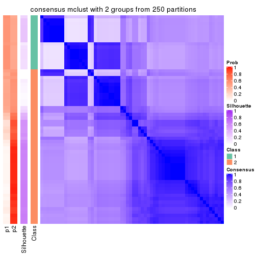
consensus_heatmap(res, k = 3)
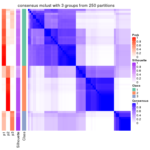
consensus_heatmap(res, k = 4)
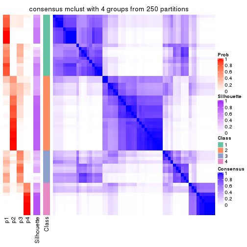
consensus_heatmap(res, k = 5)
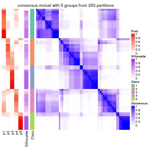
consensus_heatmap(res, k = 6)
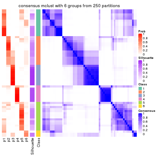
Heatmaps for the membership of samples in all partitions to see how consistent they are:
membership_heatmap(res, k = 2)
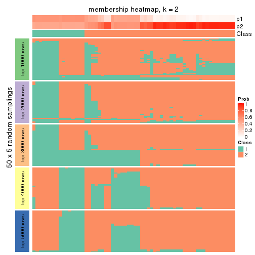
membership_heatmap(res, k = 3)
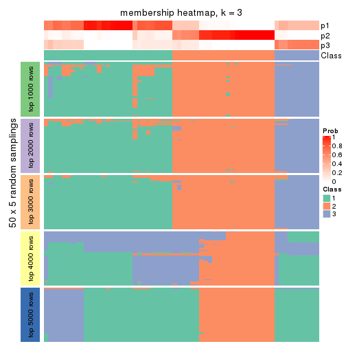
membership_heatmap(res, k = 4)
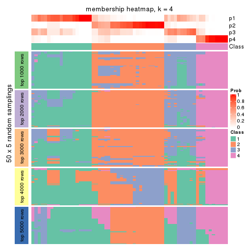
membership_heatmap(res, k = 5)
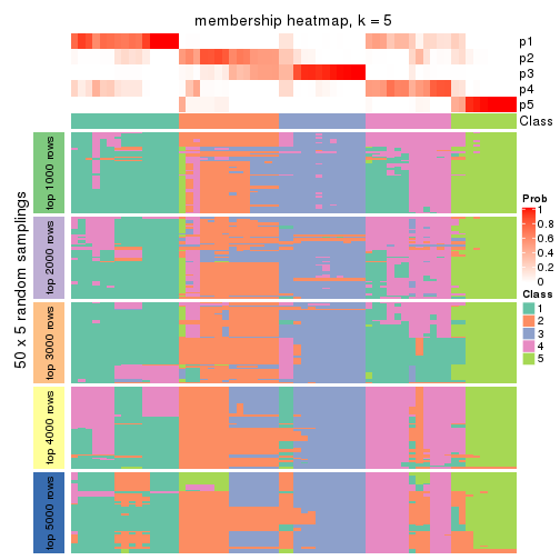
membership_heatmap(res, k = 6)
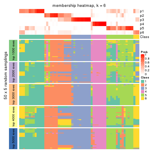
As soon as we have had the classes for columns, we can look for signatures which are significantly different between classes which can be candidate marks for certain classes. Following are the heatmaps for signatures.
Signature heatmaps where rows are scaled:
get_signatures(res, k = 2)

get_signatures(res, k = 3)
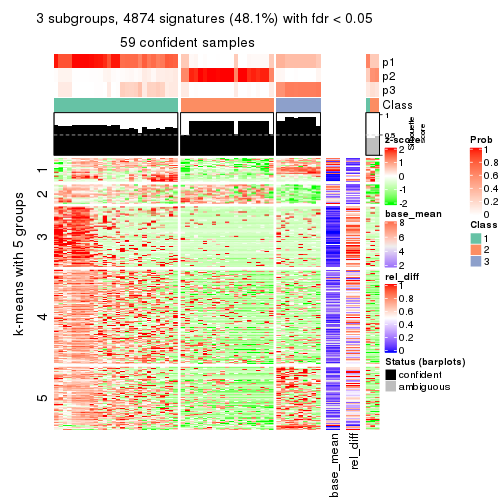
get_signatures(res, k = 4)
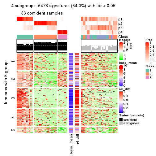
get_signatures(res, k = 5)
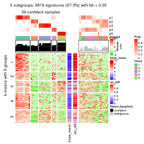
get_signatures(res, k = 6)
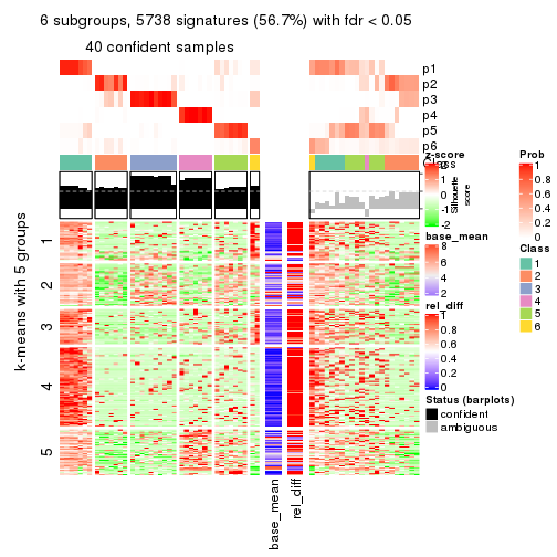
Signature heatmaps where rows are not scaled:
get_signatures(res, k = 2, scale_rows = FALSE)

get_signatures(res, k = 3, scale_rows = FALSE)
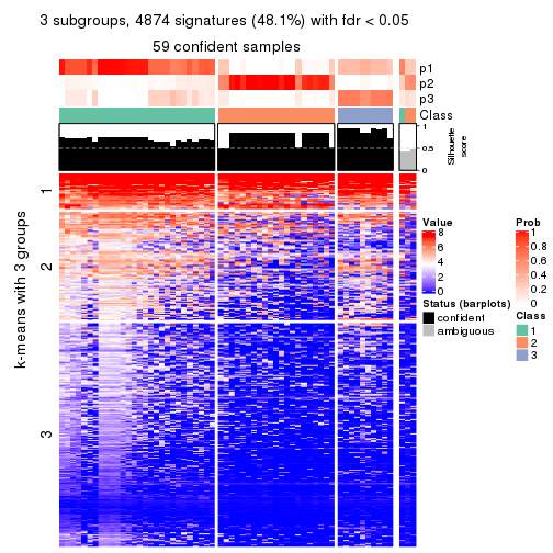
get_signatures(res, k = 4, scale_rows = FALSE)
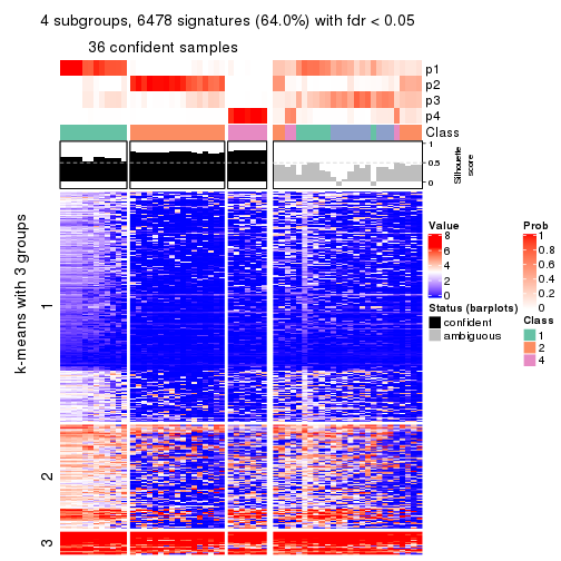
get_signatures(res, k = 5, scale_rows = FALSE)
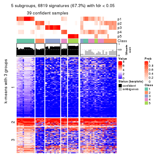
get_signatures(res, k = 6, scale_rows = FALSE)
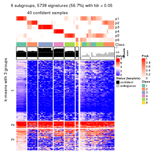
Compare the overlap of signatures from different k:
compare_signatures(res)
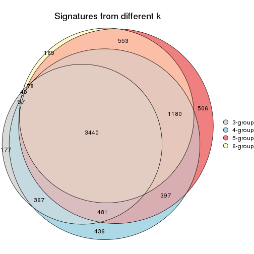
get_signature() returns a data frame invisibly. TO get the list of signatures, the function
call should be assigned to a variable explicitly. In following code, if plot argument is set
to FALSE, no heatmap is plotted while only the differential analysis is performed.
# code only for demonstration
tb = get_signature(res, k = ..., plot = FALSE)
An example of the output of tb is:
#>   which_row         fdr    mean_1    mean_2 scaled_mean_1 scaled_mean_2 km
#> 1        38 0.042760348  8.373488  9.131774    -0.5533452     0.5164555  1
#> 2        40 0.018707592  7.106213  8.469186    -0.6173731     0.5762149  1
#> 3        55 0.019134737 10.221463 11.207825    -0.6159697     0.5749050  1
#> 4        59 0.006059896  5.921854  7.869574    -0.6899429     0.6439467  1
#> 5        60 0.018055526  8.928898 10.211722    -0.6204761     0.5791110  1
#> 6        98 0.009384629 15.714769 14.887706     0.6635654    -0.6193277  2
...
The columns in tb are:
which_row: row indices corresponding to the input matrix.fdr: FDR for the differential test. mean_x: The mean value in group x.scaled_mean_x: The mean value in group x after rows are scaled.km: Row groups if k-means clustering is applied to rows.UMAP plot which shows how samples are separated.
dimension_reduction(res, k = 2, method = "UMAP")
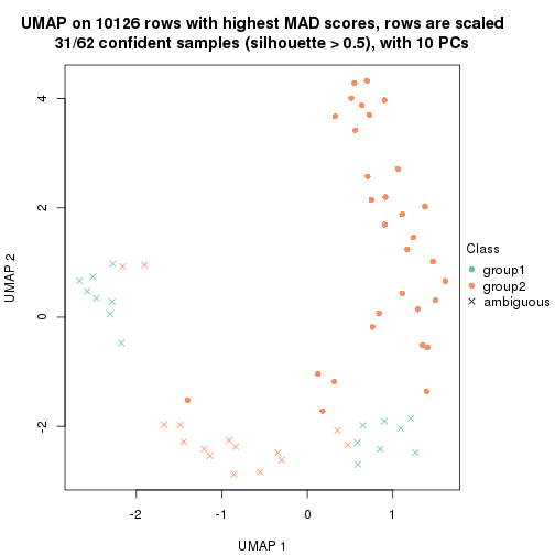
dimension_reduction(res, k = 3, method = "UMAP")
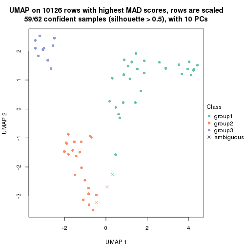
dimension_reduction(res, k = 4, method = "UMAP")
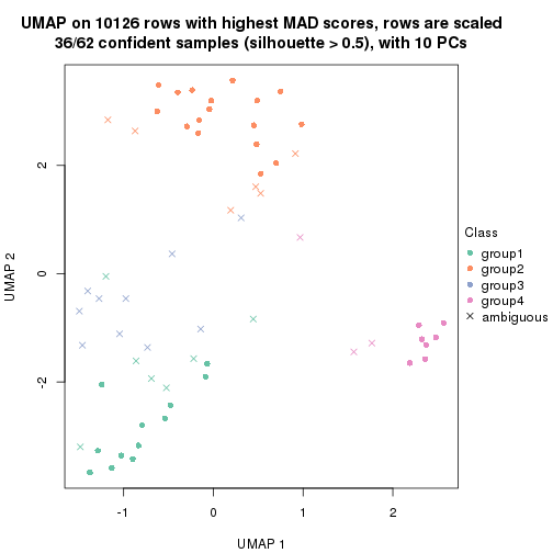
dimension_reduction(res, k = 5, method = "UMAP")
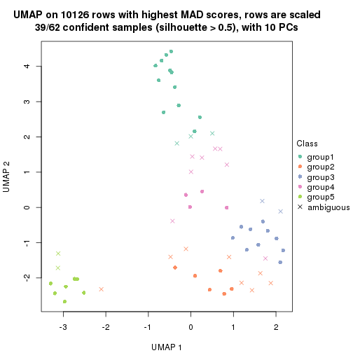
dimension_reduction(res, k = 6, method = "UMAP")
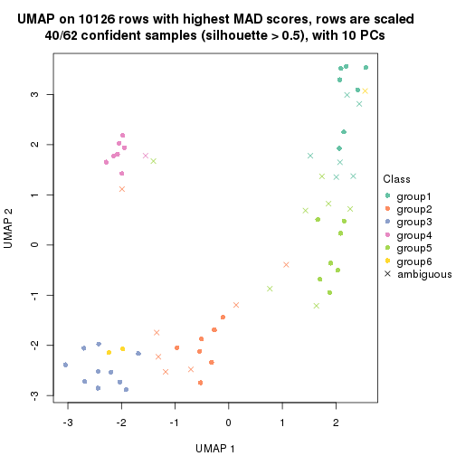
Following heatmap shows how subgroups are split when increasing k:
collect_classes(res)
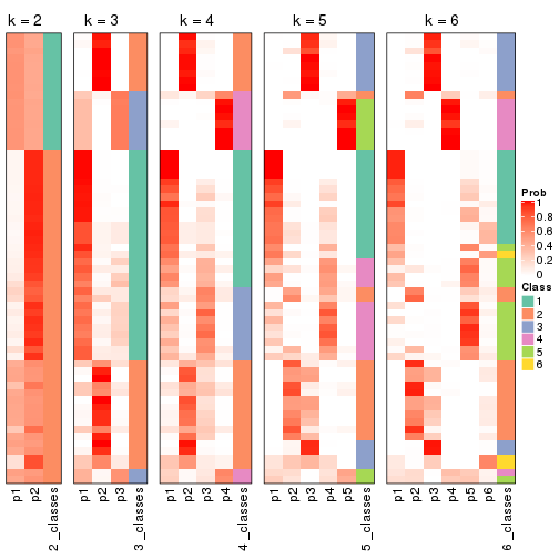
If matrix rows can be associated to genes, consider to use functional_enrichment(res,
...) to perform function enrichment for the signature genes. See this vignette for more detailed explanations.
The object with results only for a single top-value method and a single partition method can be extracted as:
res = res_list["MAD", "NMF"]
# you can also extract it by
# res = res_list["MAD:NMF"]
A summary of res and all the functions that can be applied to it:
res
#> A 'ConsensusPartition' object with k = 2, 3, 4, 5, 6.
#>   On a matrix with 10126 rows and 62 columns.
#>   Top rows (1000, 2000, 3000, 4000, 5000) are extracted by 'MAD' method.
#>   Subgroups are detected by 'NMF' method.
#>   Performed in total 1250 partitions by row resampling.
#>   Best k for subgroups seems to be 2.
#>
#> Following methods can be applied to this 'ConsensusPartition' object:
#>  [1] "cola_report"             "collect_classes"         "collect_plots"
#>  [4] "collect_stats"           "colnames"                "compare_signatures"
#>  [7] "consensus_heatmap"       "dimension_reduction"     "functional_enrichment"
#> [10] "get_anno_col"            "get_anno"                "get_classes"
#> [13] "get_consensus"           "get_matrix"              "get_membership"
#> [16] "get_param"               "get_signatures"          "get_stats"
#> [19] "is_best_k"               "is_stable_k"             "membership_heatmap"
#> [22] "ncol"                    "nrow"                    "plot_ecdf"
#> [25] "rownames"                "select_partition_number" "show"
#> [28] "suggest_best_k"          "test_to_known_factors"
collect_plots() function collects all the plots made from res for all k (number of partitions)
into one single page to provide an easy and fast comparison between different k.
collect_plots(res)
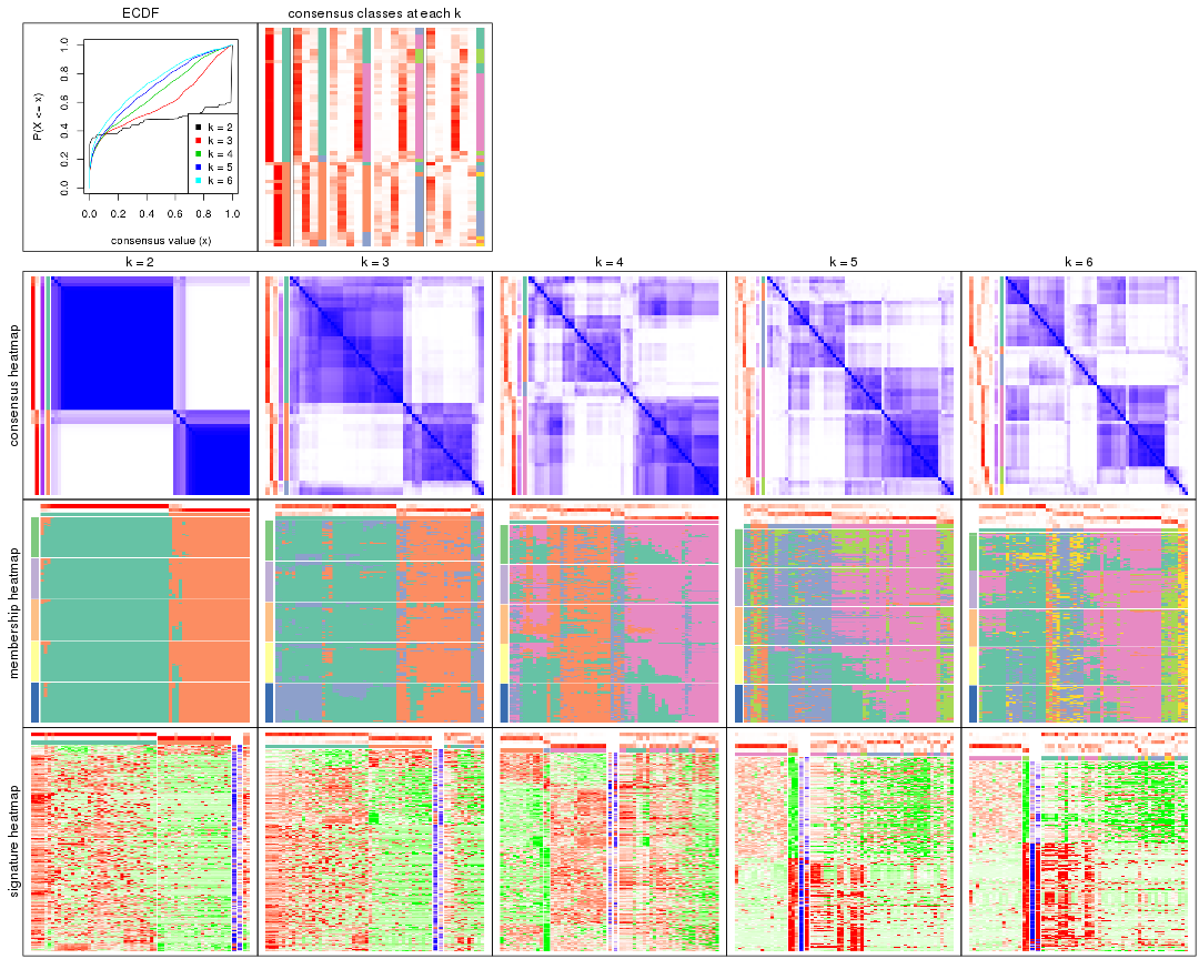
The plots are:
k and the heatmap of
predicted classes for each k.k.k.k.All the plots in panels can be made by individual functions and they are plotted later in this section.
select_partition_number() produces several plots showing different
statistics for choosing “optimized” k. There are following statistics:
k;k, the area increased is defined as \(A_k - A_{k-1}\).The detailed explanations of these statistics can be found in the cola vignette.
Generally speaking, lower PAC score, higher mean silhouette score or higher
concordance corresponds to better partition. Rand index and Jaccard index
measure how similar the current partition is compared to partition with k-1.
If they are too similar, we won't accept k is better than k-1.
select_partition_number(res)
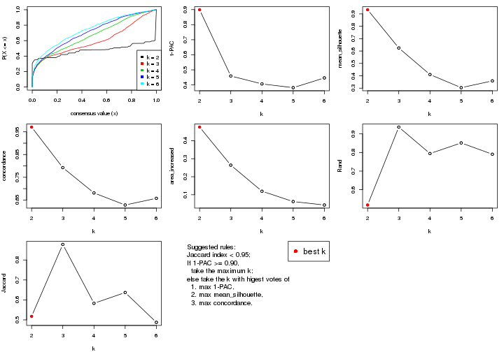
The numeric values for all these statistics can be obtained by get_stats().
get_stats(res)
#> k 1-PAC mean_silhouette concordance area_increased Rand Jaccard
#> 2 2 0.899 0.934 0.971 0.4753 0.518 0.518
#> 3 3 0.459 0.625 0.792 0.2641 0.937 0.878
#> 4 4 0.407 0.410 0.681 0.1194 0.794 0.583
#> 5 5 0.382 0.304 0.628 0.0622 0.851 0.637
#> 6 6 0.446 0.359 0.657 0.0431 0.791 0.488
suggest_best_k() suggests the best \(k\) based on these statistics. The rules are as follows:
suggest_best_k(res)
#> [1] 2
Following shows the table of the partitions (You need to click the show/hide
code output link to see it). The membership matrix (columns with name p*)
is inferred by
clue::cl_consensus()
function with the SE method. Basically the value in the membership matrix
represents the probability to belong to a certain group. The finall class
label for an item is determined with the group with highest probability it
belongs to.
In get_classes() function, the entropy is calculated from the membership
matrix and the silhouette score is calculated from the consensus matrix.
cbind(get_classes(res, k = 2), get_membership(res, k = 2))
#> class entropy silhouette p1 p2
#> SRR764776 1 0.0000 0.985 1.000 0.000
#> SRR764777 1 0.0000 0.985 1.000 0.000
#> SRR764778 1 0.0000 0.985 1.000 0.000
#> SRR764779 1 0.0000 0.985 1.000 0.000
#> SRR764780 1 0.0000 0.985 1.000 0.000
#> SRR764781 1 0.0000 0.985 1.000 0.000
#> SRR764782 1 0.0000 0.985 1.000 0.000
#> SRR764783 1 0.0000 0.985 1.000 0.000
#> SRR764784 1 0.0000 0.985 1.000 0.000
#> SRR764785 1 0.0000 0.985 1.000 0.000
#> SRR764786 1 0.0000 0.985 1.000 0.000
#> SRR764787 1 0.0000 0.985 1.000 0.000
#> SRR764788 1 0.0000 0.985 1.000 0.000
#> SRR764789 1 0.0000 0.985 1.000 0.000
#> SRR764790 1 0.0000 0.985 1.000 0.000
#> SRR764791 1 0.0376 0.982 0.996 0.004
#> SRR764792 1 0.0000 0.985 1.000 0.000
#> SRR764793 1 0.0000 0.985 1.000 0.000
#> SRR764794 1 0.0000 0.985 1.000 0.000
#> SRR764795 1 0.0000 0.985 1.000 0.000
#> SRR764796 1 0.0000 0.985 1.000 0.000
#> SRR764797 1 0.0000 0.985 1.000 0.000
#> SRR764798 2 0.0000 0.941 0.000 1.000
#> SRR764799 2 0.9358 0.489 0.352 0.648
#> SRR764800 1 0.0000 0.985 1.000 0.000
#> SRR764801 2 0.0000 0.941 0.000 1.000
#> SRR764802 1 0.0000 0.985 1.000 0.000
#> SRR764803 1 0.0000 0.985 1.000 0.000
#> SRR764804 2 0.0000 0.941 0.000 1.000
#> SRR764805 2 0.0000 0.941 0.000 1.000
#> SRR764806 2 0.0000 0.941 0.000 1.000
#> SRR764807 2 0.2603 0.911 0.044 0.956
#> SRR764808 2 0.8661 0.619 0.288 0.712
#> SRR764809 2 0.0000 0.941 0.000 1.000
#> SRR764810 2 0.0000 0.941 0.000 1.000
#> SRR764811 2 0.0000 0.941 0.000 1.000
#> SRR764812 2 0.0000 0.941 0.000 1.000
#> SRR764813 2 0.0938 0.934 0.012 0.988
#> SRR764814 1 0.4690 0.880 0.900 0.100
#> SRR764815 1 0.7056 0.754 0.808 0.192
#> SRR764816 2 0.9552 0.434 0.376 0.624
#> SRR764817 1 0.7453 0.720 0.788 0.212
#> SRR1066622 1 0.0000 0.985 1.000 0.000
#> SRR1066623 1 0.0000 0.985 1.000 0.000
#> SRR1066624 1 0.0000 0.985 1.000 0.000
#> SRR1066625 1 0.0000 0.985 1.000 0.000
#> SRR1066626 1 0.0000 0.985 1.000 0.000
#> SRR1066627 1 0.0000 0.985 1.000 0.000
#> SRR1066628 1 0.0000 0.985 1.000 0.000
#> SRR1066629 1 0.0000 0.985 1.000 0.000
#> SRR1066630 1 0.0000 0.985 1.000 0.000
#> SRR1066631 1 0.0000 0.985 1.000 0.000
#> SRR1066632 2 0.0000 0.941 0.000 1.000
#> SRR1066633 2 0.0000 0.941 0.000 1.000
#> SRR1066634 2 0.7745 0.713 0.228 0.772
#> SRR1066635 2 0.0000 0.941 0.000 1.000
#> SRR1066636 2 0.0000 0.941 0.000 1.000
#> SRR1066637 2 0.0000 0.941 0.000 1.000
#> SRR1066638 2 0.0000 0.941 0.000 1.000
#> SRR1066639 2 0.0000 0.941 0.000 1.000
#> SRR1066640 2 0.0000 0.941 0.000 1.000
#> SRR1066641 2 0.0376 0.939 0.004 0.996
cbind(get_classes(res, k = 3), get_membership(res, k = 3))
#> class entropy silhouette p1 p2 p3
#> SRR764776 1 0.4189 0.70529 0.876 0.056 0.068
#> SRR764777 1 0.3899 0.71071 0.888 0.056 0.056
#> SRR764778 1 0.2527 0.73446 0.936 0.020 0.044
#> SRR764779 1 0.2527 0.73446 0.936 0.020 0.044
#> SRR764780 1 0.2297 0.73633 0.944 0.020 0.036
#> SRR764781 1 0.1643 0.74572 0.956 0.000 0.044
#> SRR764782 1 0.0592 0.74725 0.988 0.000 0.012
#> SRR764783 1 0.3310 0.72515 0.908 0.028 0.064
#> SRR764784 1 0.1964 0.73944 0.944 0.000 0.056
#> SRR764785 1 0.6879 0.14703 0.556 0.016 0.428
#> SRR764786 1 0.6505 -0.02151 0.528 0.004 0.468
#> SRR764787 1 0.3886 0.71290 0.880 0.024 0.096
#> SRR764788 1 0.3234 0.72833 0.908 0.020 0.072
#> SRR764789 1 0.4834 0.64866 0.792 0.004 0.204
#> SRR764790 3 0.7021 0.19327 0.436 0.020 0.544
#> SRR764791 1 0.5413 0.68356 0.800 0.036 0.164
#> SRR764792 1 0.5627 0.67441 0.780 0.032 0.188
#> SRR764793 1 0.2793 0.74785 0.928 0.028 0.044
#> SRR764794 1 0.6229 0.54344 0.700 0.020 0.280
#> SRR764795 1 0.1753 0.74020 0.952 0.000 0.048
#> SRR764796 1 0.1964 0.73944 0.944 0.000 0.056
#> SRR764797 1 0.4289 0.70282 0.868 0.040 0.092
#> SRR764798 2 0.4642 0.77577 0.060 0.856 0.084
#> SRR764799 2 0.7062 0.53597 0.236 0.696 0.068
#> SRR764800 1 0.4370 0.69497 0.868 0.076 0.056
#> SRR764801 2 0.4194 0.77470 0.060 0.876 0.064
#> SRR764802 1 0.1832 0.74659 0.956 0.008 0.036
#> SRR764803 1 0.0747 0.74667 0.984 0.000 0.016
#> SRR764804 2 0.3030 0.80813 0.004 0.904 0.092
#> SRR764805 2 0.3551 0.79608 0.000 0.868 0.132
#> SRR764806 2 0.2165 0.81285 0.000 0.936 0.064
#> SRR764807 3 0.6451 0.00517 0.024 0.292 0.684
#> SRR764808 3 0.7365 0.38337 0.112 0.188 0.700
#> SRR764809 2 0.3038 0.80048 0.000 0.896 0.104
#> SRR764810 2 0.4504 0.76370 0.000 0.804 0.196
#> SRR764811 2 0.5733 0.64208 0.000 0.676 0.324
#> SRR764812 2 0.3644 0.79542 0.004 0.872 0.124
#> SRR764813 2 0.7013 0.45411 0.020 0.548 0.432
#> SRR764814 1 0.7624 0.41334 0.672 0.224 0.104
#> SRR764815 1 0.8953 0.20918 0.560 0.260 0.180
#> SRR764816 2 0.7590 0.46745 0.268 0.652 0.080
#> SRR764817 1 0.8465 0.11033 0.528 0.376 0.096
#> SRR1066622 1 0.4750 0.63698 0.784 0.000 0.216
#> SRR1066623 1 0.5178 0.59115 0.744 0.000 0.256
#> SRR1066624 1 0.2711 0.72318 0.912 0.000 0.088
#> SRR1066625 1 0.4291 0.67331 0.820 0.000 0.180
#> SRR1066626 1 0.4931 0.62056 0.768 0.000 0.232
#> SRR1066627 1 0.5098 0.59996 0.752 0.000 0.248
#> SRR1066628 1 0.4974 0.61511 0.764 0.000 0.236
#> SRR1066629 1 0.4605 0.64926 0.796 0.000 0.204
#> SRR1066630 3 0.6308 -0.02012 0.492 0.000 0.508
#> SRR1066631 1 0.5291 0.57238 0.732 0.000 0.268
#> SRR1066632 2 0.3148 0.80944 0.036 0.916 0.048
#> SRR1066633 2 0.3237 0.80302 0.032 0.912 0.056
#> SRR1066634 2 0.7297 0.58168 0.188 0.704 0.108
#> SRR1066635 2 0.2711 0.81266 0.000 0.912 0.088
#> SRR1066636 2 0.2550 0.81200 0.024 0.936 0.040
#> SRR1066637 2 0.3039 0.80673 0.036 0.920 0.044
#> SRR1066638 2 0.2301 0.81676 0.004 0.936 0.060
#> SRR1066639 2 0.3120 0.81655 0.012 0.908 0.080
#> SRR1066640 2 0.3850 0.81094 0.028 0.884 0.088
#> SRR1066641 2 0.6799 0.43253 0.012 0.532 0.456
cbind(get_classes(res, k = 4), get_membership(res, k = 4))
#> class entropy silhouette p1 p2 p3 p4
#> SRR764776 1 0.5929 0.1783 0.520 0.028 0.004 0.448
#> SRR764777 1 0.5863 0.1041 0.496 0.024 0.004 0.476
#> SRR764778 4 0.5273 0.0104 0.456 0.008 0.000 0.536
#> SRR764779 4 0.5281 -0.0211 0.464 0.008 0.000 0.528
#> SRR764780 4 0.4643 0.3648 0.344 0.000 0.000 0.656
#> SRR764781 4 0.3764 0.5674 0.216 0.000 0.000 0.784
#> SRR764782 4 0.3810 0.5957 0.188 0.000 0.008 0.804
#> SRR764783 4 0.5172 0.2123 0.404 0.008 0.000 0.588
#> SRR764784 4 0.2831 0.6297 0.120 0.000 0.004 0.876
#> SRR764785 1 0.7910 0.2020 0.364 0.000 0.316 0.320
#> SRR764786 1 0.8026 0.1435 0.372 0.004 0.276 0.348
#> SRR764787 4 0.6133 0.2344 0.384 0.012 0.032 0.572
#> SRR764788 4 0.5666 0.0266 0.460 0.016 0.004 0.520
#> SRR764789 4 0.5037 0.4893 0.196 0.008 0.040 0.756
#> SRR764790 4 0.7915 -0.1753 0.168 0.016 0.400 0.416
#> SRR764791 4 0.5036 0.5158 0.192 0.036 0.012 0.760
#> SRR764792 4 0.7994 -0.1817 0.384 0.076 0.072 0.468
#> SRR764793 4 0.5992 0.3955 0.272 0.040 0.020 0.668
#> SRR764794 1 0.8144 0.1916 0.396 0.020 0.192 0.392
#> SRR764795 4 0.2593 0.6353 0.104 0.000 0.004 0.892
#> SRR764796 4 0.2334 0.6374 0.088 0.000 0.004 0.908
#> SRR764797 1 0.5328 0.0213 0.520 0.004 0.004 0.472
#> SRR764798 2 0.5558 0.5283 0.364 0.608 0.028 0.000
#> SRR764799 2 0.6177 0.2560 0.468 0.488 0.004 0.040
#> SRR764800 1 0.6668 0.2141 0.480 0.072 0.004 0.444
#> SRR764801 2 0.5298 0.5355 0.372 0.612 0.016 0.000
#> SRR764802 4 0.3688 0.5782 0.208 0.000 0.000 0.792
#> SRR764803 4 0.3528 0.5947 0.192 0.000 0.000 0.808
#> SRR764804 2 0.2282 0.6021 0.024 0.924 0.052 0.000
#> SRR764805 2 0.4700 0.4488 0.084 0.792 0.124 0.000
#> SRR764806 2 0.4036 0.6036 0.088 0.836 0.076 0.000
#> SRR764807 3 0.5741 0.6072 0.116 0.144 0.732 0.008
#> SRR764808 3 0.7561 0.5299 0.152 0.092 0.636 0.120
#> SRR764809 2 0.3996 0.4926 0.060 0.836 0.104 0.000
#> SRR764810 2 0.5520 0.2690 0.060 0.696 0.244 0.000
#> SRR764811 2 0.7043 -0.3218 0.120 0.456 0.424 0.000
#> SRR764812 2 0.3464 0.5770 0.032 0.860 0.108 0.000
#> SRR764813 3 0.7486 0.4677 0.188 0.348 0.464 0.000
#> SRR764814 1 0.7180 0.4165 0.588 0.148 0.012 0.252
#> SRR764815 1 0.9057 0.3797 0.464 0.136 0.144 0.256
#> SRR764816 1 0.6315 -0.3124 0.480 0.468 0.004 0.048
#> SRR764817 1 0.7080 0.1366 0.544 0.324 0.004 0.128
#> SRR1066622 4 0.0188 0.6346 0.000 0.000 0.004 0.996
#> SRR1066623 4 0.1174 0.6223 0.012 0.000 0.020 0.968
#> SRR1066624 4 0.2179 0.6386 0.064 0.000 0.012 0.924
#> SRR1066625 4 0.1520 0.6320 0.024 0.000 0.020 0.956
#> SRR1066626 4 0.0927 0.6270 0.008 0.000 0.016 0.976
#> SRR1066627 4 0.1624 0.6108 0.020 0.000 0.028 0.952
#> SRR1066628 4 0.1059 0.6240 0.016 0.000 0.012 0.972
#> SRR1066629 4 0.0376 0.6355 0.004 0.000 0.004 0.992
#> SRR1066630 4 0.6258 0.2742 0.104 0.008 0.212 0.676
#> SRR1066631 4 0.1936 0.6007 0.028 0.000 0.032 0.940
#> SRR1066632 2 0.3625 0.6711 0.160 0.828 0.012 0.000
#> SRR1066633 2 0.4567 0.6382 0.276 0.716 0.008 0.000
#> SRR1066634 2 0.6919 0.4944 0.316 0.588 0.028 0.068
#> SRR1066635 2 0.5783 0.5983 0.160 0.720 0.116 0.004
#> SRR1066636 2 0.4290 0.6647 0.212 0.772 0.016 0.000
#> SRR1066637 2 0.4319 0.6589 0.228 0.760 0.012 0.000
#> SRR1066638 2 0.4072 0.6520 0.120 0.828 0.052 0.000
#> SRR1066639 2 0.3763 0.6663 0.144 0.832 0.024 0.000
#> SRR1066640 2 0.4881 0.6614 0.196 0.756 0.048 0.000
#> SRR1066641 3 0.7119 0.4294 0.140 0.352 0.508 0.000
cbind(get_classes(res, k = 5), get_membership(res, k = 5))
#> class entropy silhouette p1 p2 p3 p4 p5
#> SRR764776 4 0.821 0.1266 0.260 0.000 0.292 0.336 0.112
#> SRR764777 4 0.816 0.2134 0.260 0.000 0.236 0.384 0.120
#> SRR764778 4 0.765 0.3617 0.244 0.000 0.152 0.488 0.116
#> SRR764779 4 0.768 0.3575 0.244 0.000 0.152 0.484 0.120
#> SRR764780 4 0.666 0.4664 0.212 0.000 0.088 0.604 0.096
#> SRR764781 4 0.475 0.5507 0.156 0.000 0.036 0.760 0.048
#> SRR764782 4 0.523 0.5327 0.084 0.000 0.044 0.736 0.136
#> SRR764783 4 0.775 0.3663 0.216 0.000 0.144 0.488 0.152
#> SRR764784 4 0.240 0.5690 0.036 0.000 0.012 0.912 0.040
#> SRR764785 5 0.602 0.5510 0.036 0.056 0.060 0.140 0.708
#> SRR764786 5 0.480 0.5355 0.008 0.028 0.032 0.180 0.752
#> SRR764787 4 0.704 0.0118 0.088 0.008 0.052 0.444 0.408
#> SRR764788 4 0.804 0.3074 0.204 0.004 0.128 0.456 0.208
#> SRR764789 4 0.525 0.3141 0.012 0.004 0.032 0.624 0.328
#> SRR764790 5 0.828 0.0956 0.044 0.196 0.052 0.284 0.424
#> SRR764791 4 0.593 0.4483 0.036 0.012 0.200 0.676 0.076
#> SRR764792 4 0.832 -0.1715 0.068 0.020 0.252 0.352 0.308
#> SRR764793 4 0.675 0.4435 0.088 0.000 0.188 0.604 0.120
#> SRR764794 5 0.719 0.5862 0.052 0.024 0.148 0.192 0.584
#> SRR764795 4 0.221 0.5674 0.028 0.000 0.004 0.916 0.052
#> SRR764796 4 0.110 0.5645 0.012 0.000 0.012 0.968 0.008
#> SRR764797 4 0.847 0.2013 0.240 0.004 0.188 0.376 0.192
#> SRR764798 3 0.505 0.3832 0.392 0.012 0.580 0.008 0.008
#> SRR764799 3 0.584 0.4169 0.296 0.008 0.616 0.064 0.016
#> SRR764800 4 0.794 0.1415 0.264 0.000 0.312 0.348 0.076
#> SRR764801 3 0.457 0.4120 0.332 0.016 0.648 0.004 0.000
#> SRR764802 4 0.445 0.5611 0.128 0.000 0.036 0.788 0.048
#> SRR764803 4 0.446 0.5588 0.096 0.000 0.028 0.792 0.084
#> SRR764804 3 0.647 -0.2595 0.248 0.144 0.580 0.000 0.028
#> SRR764805 3 0.691 -0.5993 0.408 0.120 0.432 0.000 0.040
#> SRR764806 3 0.581 -0.3535 0.352 0.060 0.568 0.000 0.020
#> SRR764807 2 0.683 0.3723 0.156 0.544 0.040 0.000 0.260
#> SRR764808 2 0.734 0.2828 0.080 0.468 0.032 0.048 0.372
#> SRR764809 1 0.579 0.4159 0.464 0.076 0.456 0.000 0.004
#> SRR764810 1 0.716 0.2892 0.488 0.236 0.240 0.000 0.036
#> SRR764811 2 0.757 -0.0812 0.340 0.400 0.204 0.000 0.056
#> SRR764812 3 0.730 -0.3107 0.248 0.172 0.512 0.000 0.068
#> SRR764813 2 0.830 0.1858 0.172 0.352 0.172 0.000 0.304
#> SRR764814 3 0.846 -0.0800 0.272 0.008 0.372 0.212 0.136
#> SRR764815 5 0.864 0.4412 0.132 0.048 0.224 0.148 0.448
#> SRR764816 3 0.541 0.4121 0.272 0.000 0.648 0.068 0.012
#> SRR764817 3 0.654 0.2902 0.268 0.000 0.580 0.100 0.052
#> SRR1066622 4 0.115 0.5464 0.008 0.004 0.000 0.964 0.024
#> SRR1066623 4 0.165 0.5318 0.012 0.008 0.000 0.944 0.036
#> SRR1066624 4 0.128 0.5517 0.016 0.004 0.000 0.960 0.020
#> SRR1066625 4 0.184 0.5273 0.012 0.012 0.000 0.936 0.040
#> SRR1066626 4 0.165 0.5353 0.008 0.012 0.000 0.944 0.036
#> SRR1066627 4 0.213 0.5157 0.016 0.016 0.000 0.924 0.044
#> SRR1066628 4 0.167 0.5328 0.016 0.008 0.000 0.944 0.032
#> SRR1066629 4 0.124 0.5436 0.008 0.004 0.000 0.960 0.028
#> SRR1066630 4 0.686 -0.0246 0.036 0.160 0.016 0.596 0.192
#> SRR1066631 4 0.223 0.5125 0.016 0.020 0.000 0.920 0.044
#> SRR1066632 3 0.422 0.2450 0.120 0.080 0.792 0.000 0.008
#> SRR1066633 3 0.375 0.4279 0.100 0.052 0.832 0.000 0.016
#> SRR1066634 3 0.513 0.4290 0.088 0.016 0.768 0.088 0.040
#> SRR1066635 3 0.586 -0.3256 0.372 0.044 0.556 0.004 0.024
#> SRR1066636 3 0.236 0.3843 0.020 0.064 0.908 0.000 0.008
#> SRR1066637 3 0.214 0.3931 0.028 0.048 0.920 0.000 0.004
#> SRR1066638 3 0.393 0.2248 0.152 0.040 0.800 0.000 0.008
#> SRR1066639 3 0.359 0.2819 0.104 0.052 0.836 0.000 0.008
#> SRR1066640 3 0.385 0.3012 0.160 0.024 0.804 0.004 0.008
#> SRR1066641 2 0.731 0.2325 0.200 0.540 0.164 0.000 0.096
cbind(get_classes(res, k = 6), get_membership(res, k = 6))
#> class entropy silhouette p1 p2 p3 p4 p5 p6
#> SRR764776 1 0.4592 0.3686 0.664 0.000 0.000 0.256 0.080 0.000
#> SRR764777 1 0.4943 0.3425 0.632 0.004 0.000 0.272 0.092 0.000
#> SRR764778 1 0.5555 0.0733 0.500 0.004 0.000 0.372 0.124 0.000
#> SRR764779 1 0.5380 0.1121 0.524 0.004 0.000 0.368 0.104 0.000
#> SRR764780 4 0.5362 0.3556 0.344 0.004 0.000 0.544 0.108 0.000
#> SRR764781 4 0.3943 0.6279 0.184 0.004 0.000 0.756 0.056 0.000
#> SRR764782 4 0.4870 0.5622 0.120 0.004 0.000 0.684 0.188 0.004
#> SRR764783 4 0.5958 0.1124 0.408 0.008 0.000 0.436 0.144 0.004
#> SRR764784 4 0.2716 0.6831 0.044 0.004 0.000 0.880 0.064 0.008
#> SRR764785 5 0.2806 0.5440 0.028 0.016 0.000 0.056 0.884 0.016
#> SRR764786 5 0.3947 0.4932 0.032 0.060 0.000 0.064 0.820 0.024
#> SRR764787 5 0.5180 0.4577 0.100 0.004 0.000 0.276 0.616 0.004
#> SRR764788 4 0.6275 0.1403 0.328 0.004 0.000 0.408 0.256 0.004
#> SRR764789 4 0.5476 0.2182 0.068 0.004 0.008 0.544 0.368 0.008
#> SRR764790 2 0.7106 0.3722 0.080 0.496 0.004 0.212 0.196 0.012
#> SRR764791 4 0.5739 0.3824 0.320 0.016 0.008 0.564 0.088 0.004
#> SRR764792 1 0.6309 -0.0662 0.420 0.008 0.000 0.232 0.336 0.004
#> SRR764793 4 0.5959 0.2820 0.356 0.000 0.008 0.504 0.116 0.016
#> SRR764794 5 0.5092 0.5777 0.180 0.028 0.004 0.076 0.704 0.008
#> SRR764795 4 0.2968 0.6792 0.060 0.004 0.000 0.864 0.064 0.008
#> SRR764796 4 0.1700 0.6946 0.028 0.000 0.000 0.936 0.024 0.012
#> SRR764797 1 0.5808 0.2305 0.540 0.008 0.000 0.252 0.200 0.000
#> SRR764798 1 0.4017 0.3125 0.776 0.012 0.152 0.000 0.004 0.056
#> SRR764799 1 0.1296 0.4533 0.952 0.000 0.032 0.000 0.004 0.012
#> SRR764800 1 0.4488 0.3750 0.664 0.000 0.000 0.280 0.052 0.004
#> SRR764801 1 0.3258 0.3679 0.832 0.016 0.120 0.000 0.000 0.032
#> SRR764802 4 0.3992 0.6289 0.176 0.004 0.000 0.756 0.064 0.000
#> SRR764803 4 0.4162 0.6270 0.144 0.004 0.000 0.752 0.100 0.000
#> SRR764804 3 0.5239 0.4394 0.240 0.060 0.660 0.000 0.012 0.028
#> SRR764805 3 0.6072 0.3029 0.084 0.080 0.640 0.000 0.024 0.172
#> SRR764806 3 0.6511 0.3533 0.256 0.016 0.472 0.000 0.012 0.244
#> SRR764807 6 0.7613 0.1329 0.012 0.300 0.104 0.000 0.256 0.328
#> SRR764808 2 0.5365 0.1732 0.024 0.732 0.048 0.024 0.120 0.052
#> SRR764809 3 0.5816 0.3238 0.096 0.056 0.596 0.000 0.000 0.252
#> SRR764810 3 0.6069 -0.0580 0.028 0.076 0.504 0.000 0.020 0.372
#> SRR764811 6 0.6396 0.3464 0.052 0.204 0.116 0.004 0.024 0.600
#> SRR764812 3 0.6520 0.4046 0.252 0.084 0.568 0.000 0.048 0.048
#> SRR764813 3 0.8218 -0.2731 0.036 0.204 0.292 0.000 0.184 0.284
#> SRR764814 1 0.5323 0.3824 0.688 0.004 0.012 0.160 0.116 0.020
#> SRR764815 5 0.6889 0.4888 0.264 0.028 0.056 0.080 0.548 0.024
#> SRR764816 1 0.1198 0.4557 0.960 0.004 0.020 0.000 0.004 0.012
#> SRR764817 1 0.1710 0.4832 0.936 0.000 0.004 0.028 0.028 0.004
#> SRR1066622 4 0.0405 0.6943 0.000 0.008 0.000 0.988 0.000 0.004
#> SRR1066623 4 0.0922 0.6849 0.000 0.024 0.004 0.968 0.004 0.000
#> SRR1066624 4 0.1837 0.6801 0.020 0.044 0.004 0.928 0.004 0.000
#> SRR1066625 4 0.2019 0.6475 0.004 0.072 0.004 0.912 0.004 0.004
#> SRR1066626 4 0.0632 0.6916 0.000 0.024 0.000 0.976 0.000 0.000
#> SRR1066627 4 0.1371 0.6721 0.000 0.040 0.004 0.948 0.004 0.004
#> SRR1066628 4 0.0862 0.6909 0.000 0.016 0.004 0.972 0.000 0.008
#> SRR1066629 4 0.0653 0.6919 0.000 0.012 0.004 0.980 0.004 0.000
#> SRR1066630 4 0.6018 -0.1571 0.012 0.340 0.020 0.544 0.068 0.016
#> SRR1066631 4 0.1699 0.6543 0.000 0.060 0.004 0.928 0.004 0.004
#> SRR1066632 3 0.4732 0.3402 0.416 0.020 0.548 0.000 0.004 0.012
#> SRR1066633 1 0.3807 0.3431 0.792 0.044 0.148 0.000 0.008 0.008
#> SRR1066634 1 0.5608 0.2762 0.676 0.016 0.192 0.020 0.024 0.072
#> SRR1066635 3 0.7145 0.3333 0.336 0.036 0.348 0.004 0.012 0.264
#> SRR1066636 1 0.4824 0.1155 0.656 0.036 0.280 0.000 0.004 0.024
#> SRR1066637 1 0.4993 -0.0157 0.608 0.024 0.324 0.000 0.000 0.044
#> SRR1066638 1 0.6234 -0.2393 0.496 0.012 0.312 0.000 0.012 0.168
#> SRR1066639 1 0.6074 -0.1741 0.532 0.048 0.324 0.000 0.004 0.092
#> SRR1066640 1 0.5714 -0.0503 0.552 0.020 0.324 0.000 0.004 0.100
#> SRR1066641 6 0.6795 0.3994 0.040 0.176 0.128 0.000 0.080 0.576
Heatmaps for the consensus matrix. It visualizes the probability of two samples to be in a same group.
consensus_heatmap(res, k = 2)
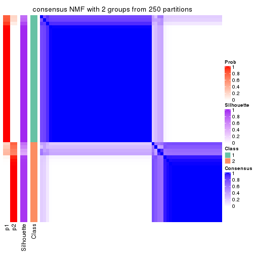
consensus_heatmap(res, k = 3)
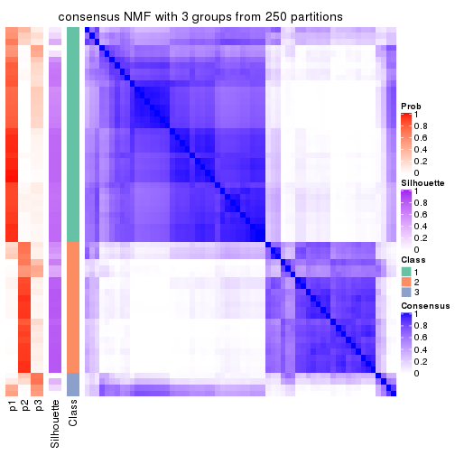
consensus_heatmap(res, k = 4)
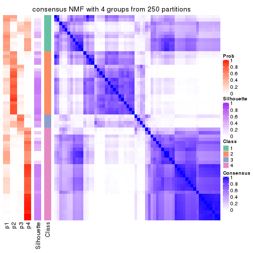
consensus_heatmap(res, k = 5)
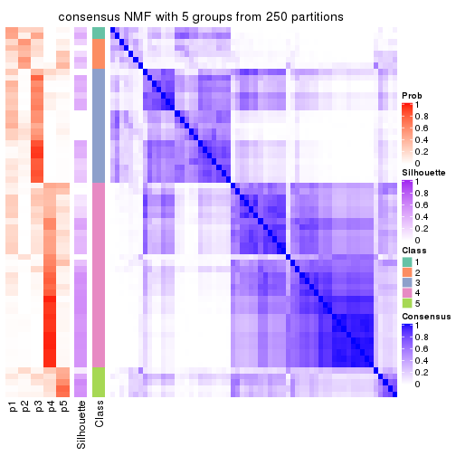
consensus_heatmap(res, k = 6)
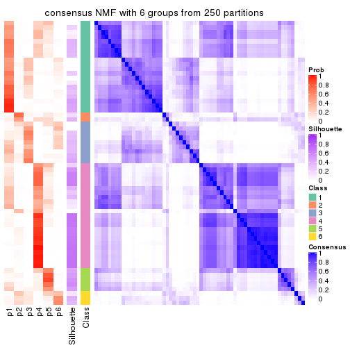
Heatmaps for the membership of samples in all partitions to see how consistent they are:
membership_heatmap(res, k = 2)
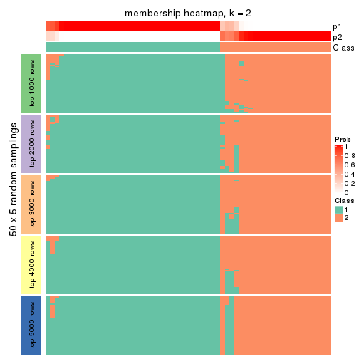
membership_heatmap(res, k = 3)
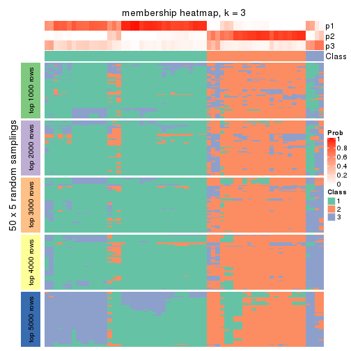
membership_heatmap(res, k = 4)
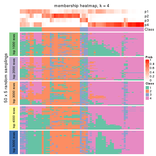
membership_heatmap(res, k = 5)
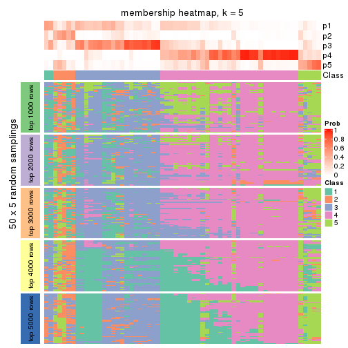
membership_heatmap(res, k = 6)
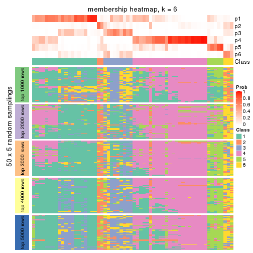
As soon as we have had the classes for columns, we can look for signatures which are significantly different between classes which can be candidate marks for certain classes. Following are the heatmaps for signatures.
Signature heatmaps where rows are scaled:
get_signatures(res, k = 2)
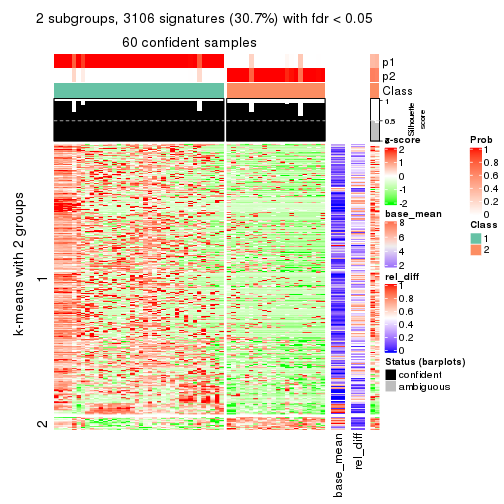
get_signatures(res, k = 3)
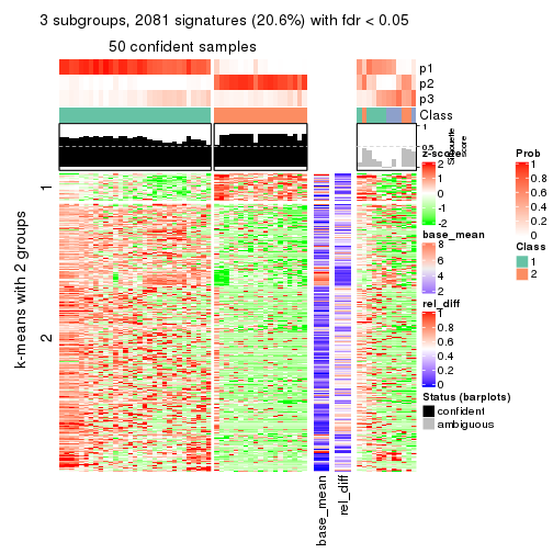
get_signatures(res, k = 4)
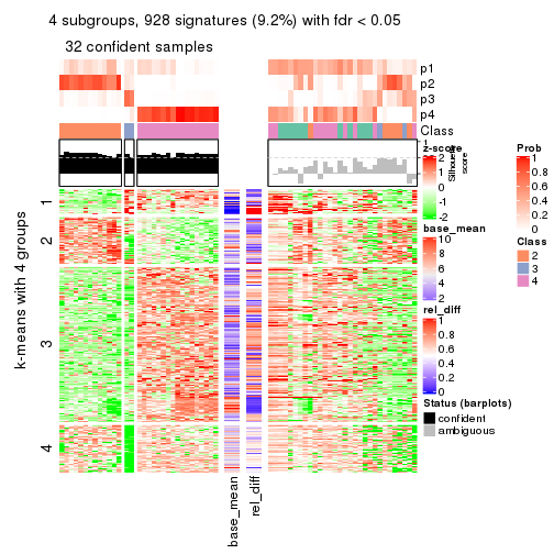
get_signatures(res, k = 5)
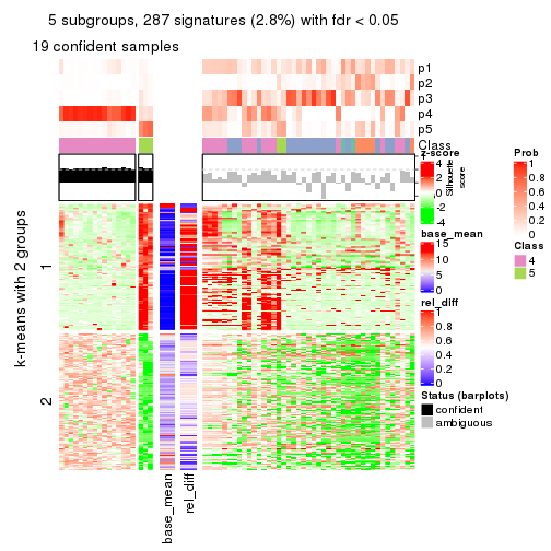
get_signatures(res, k = 6)
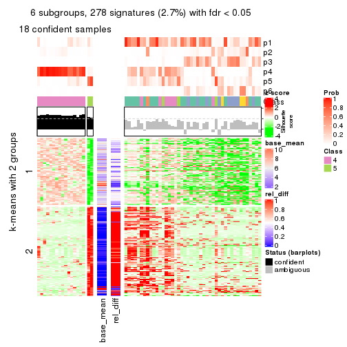
Signature heatmaps where rows are not scaled:
get_signatures(res, k = 2, scale_rows = FALSE)
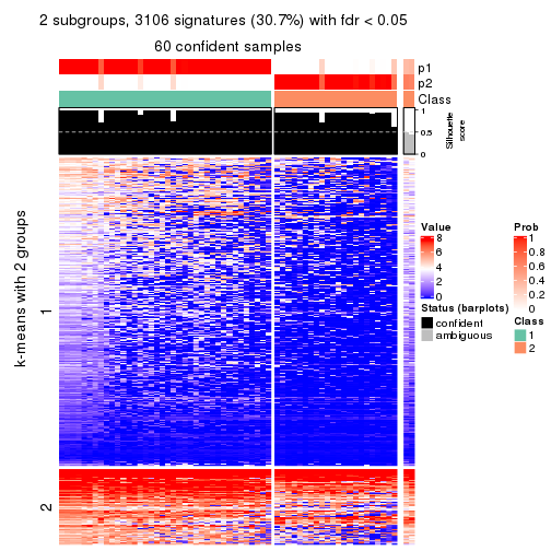
get_signatures(res, k = 3, scale_rows = FALSE)
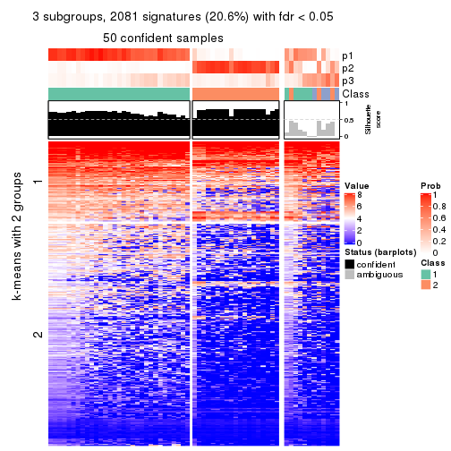
get_signatures(res, k = 4, scale_rows = FALSE)
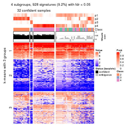
get_signatures(res, k = 5, scale_rows = FALSE)
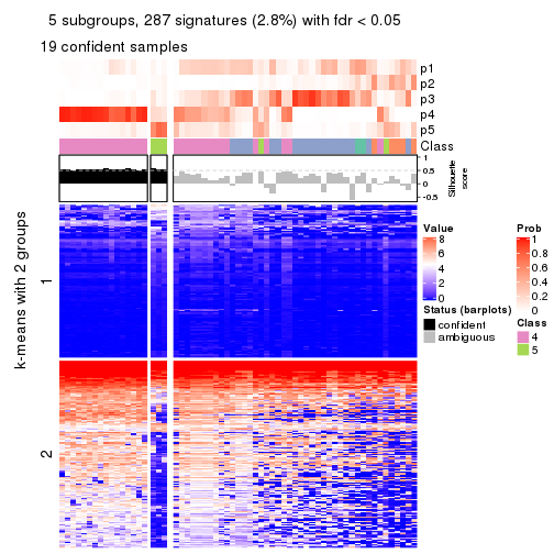
get_signatures(res, k = 6, scale_rows = FALSE)
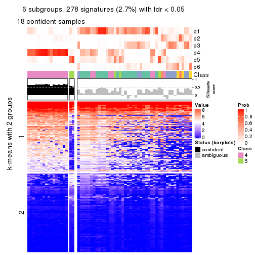
Compare the overlap of signatures from different k:
compare_signatures(res)
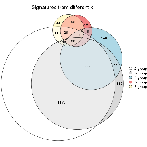
get_signature() returns a data frame invisibly. TO get the list of signatures, the function
call should be assigned to a variable explicitly. In following code, if plot argument is set
to FALSE, no heatmap is plotted while only the differential analysis is performed.
# code only for demonstration
tb = get_signature(res, k = ..., plot = FALSE)
An example of the output of tb is:
#> which_row fdr mean_1 mean_2 scaled_mean_1 scaled_mean_2 km
#> 1 38 0.042760348 8.373488 9.131774 -0.5533452 0.5164555 1
#> 2 40 0.018707592 7.106213 8.469186 -0.6173731 0.5762149 1
#> 3 55 0.019134737 10.221463 11.207825 -0.6159697 0.5749050 1
#> 4 59 0.006059896 5.921854 7.869574 -0.6899429 0.6439467 1
#> 5 60 0.018055526 8.928898 10.211722 -0.6204761 0.5791110 1
#> 6 98 0.009384629 15.714769 14.887706 0.6635654 -0.6193277 2
...
The columns in tb are:
which_row: row indices corresponding to the input matrix.fdr: FDR for the differential test. mean_x: The mean value in group x.scaled_mean_x: The mean value in group x after rows are scaled.km: Row groups if k-means clustering is applied to rows.UMAP plot which shows how samples are separated.
dimension_reduction(res, k = 2, method = "UMAP")
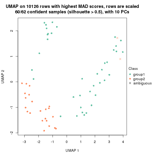
dimension_reduction(res, k = 3, method = "UMAP")
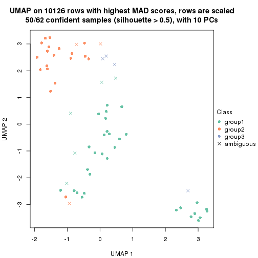
dimension_reduction(res, k = 4, method = "UMAP")
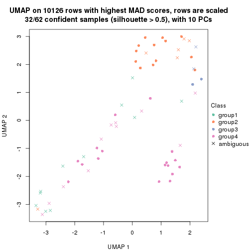
dimension_reduction(res, k = 5, method = "UMAP")
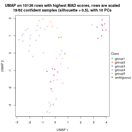
dimension_reduction(res, k = 6, method = "UMAP")
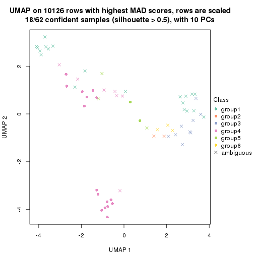
Following heatmap shows how subgroups are split when increasing k:
collect_classes(res)

If matrix rows can be associated to genes, consider to use functional_enrichment(res,
...) to perform function enrichment for the signature genes. See this vignette for more detailed explanations.
The object with results only for a single top-value method and a single partition method can be extracted as:
res = res_list["ATC", "hclust"]
# you can also extract it by
# res = res_list["ATC:hclust"]
A summary of res and all the functions that can be applied to it:
res
#> A 'ConsensusPartition' object with k = 2, 3, 4, 5, 6.
#> On a matrix with 10126 rows and 62 columns.
#> Top rows (1000, 2000, 3000, 4000, 5000) are extracted by 'ATC' method.
#> Subgroups are detected by 'hclust' method.
#> Performed in total 1250 partitions by row resampling.
#> Best k for subgroups seems to be 3.
#>
#> Following methods can be applied to this 'ConsensusPartition' object:
#> [1] "cola_report" "collect_classes" "collect_plots"
#> [4] "collect_stats" "colnames" "compare_signatures"
#> [7] "consensus_heatmap" "dimension_reduction" "functional_enrichment"
#> [10] "get_anno_col" "get_anno" "get_classes"
#> [13] "get_consensus" "get_matrix" "get_membership"
#> [16] "get_param" "get_signatures" "get_stats"
#> [19] "is_best_k" "is_stable_k" "membership_heatmap"
#> [22] "ncol" "nrow" "plot_ecdf"
#> [25] "rownames" "select_partition_number" "show"
#> [28] "suggest_best_k" "test_to_known_factors"
collect_plots() function collects all the plots made from res for all k (number of partitions)
into one single page to provide an easy and fast comparison between different k.
collect_plots(res)
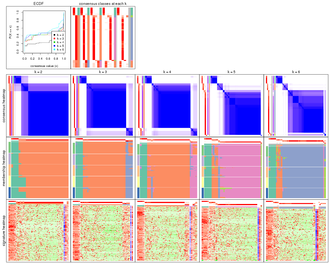
The plots are:
k and the heatmap of
predicted classes for each k.k.k.k.All the plots in panels can be made by individual functions and they are plotted later in this section.
select_partition_number() produces several plots showing different
statistics for choosing “optimized” k. There are following statistics:
k;k, the area increased is defined as \(A_k - A_{k-1}\).The detailed explanations of these statistics can be found in the cola vignette.
Generally speaking, lower PAC score, higher mean silhouette score or higher
concordance corresponds to better partition. Rand index and Jaccard index
measure how similar the current partition is compared to partition with k-1.
If they are too similar, we won't accept k is better than k-1.
select_partition_number(res)
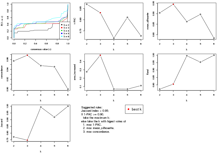
The numeric values for all these statistics can be obtained by get_stats().
get_stats(res)
#> k 1-PAC mean_silhouette concordance area_increased Rand Jaccard
#> 2 2 0.869 0.904 0.957 0.2768 0.772 0.772
#> 3 3 0.831 0.945 0.969 0.4741 0.805 0.748
#> 4 4 0.718 0.862 0.948 0.0708 0.996 0.994
#> 5 5 0.811 0.897 0.945 0.0695 0.953 0.919
#> 6 6 0.728 0.784 0.900 0.1112 1.000 1.000
suggest_best_k() suggests the best \(k\) based on these statistics. The rules are as follows:
suggest_best_k(res)
#> [1] 3
Following shows the table of the partitions (You need to click the show/hide
code output link to see it). The membership matrix (columns with name p*)
is inferred by
clue::cl_consensus()
function with the SE method. Basically the value in the membership matrix
represents the probability to belong to a certain group. The finall class
label for an item is determined with the group with highest probability it
belongs to.
In get_classes() function, the entropy is calculated from the membership
matrix and the silhouette score is calculated from the consensus matrix.
cbind(get_classes(res, k = 2), get_membership(res, k = 2))
#> class entropy silhouette p1 p2
#> SRR764776 1 0.0000 0.978 1.000 0.000
#> SRR764777 1 0.0000 0.978 1.000 0.000
#> SRR764778 1 0.0000 0.978 1.000 0.000
#> SRR764779 1 0.0000 0.978 1.000 0.000
#> SRR764780 2 0.9491 0.482 0.368 0.632
#> SRR764781 2 0.9491 0.482 0.368 0.632
#> SRR764782 2 0.0000 0.949 0.000 1.000
#> SRR764783 2 0.8661 0.631 0.288 0.712
#> SRR764784 2 0.0000 0.949 0.000 1.000
#> SRR764785 2 0.0000 0.949 0.000 1.000
#> SRR764786 2 0.0000 0.949 0.000 1.000
#> SRR764787 2 0.0000 0.949 0.000 1.000
#> SRR764788 2 0.0000 0.949 0.000 1.000
#> SRR764789 2 0.0000 0.949 0.000 1.000
#> SRR764790 2 0.0000 0.949 0.000 1.000
#> SRR764791 2 0.0000 0.949 0.000 1.000
#> SRR764792 2 0.0000 0.949 0.000 1.000
#> SRR764793 2 0.0000 0.949 0.000 1.000
#> SRR764794 2 0.0000 0.949 0.000 1.000
#> SRR764795 2 0.0000 0.949 0.000 1.000
#> SRR764796 2 0.0000 0.949 0.000 1.000
#> SRR764797 2 0.8661 0.631 0.288 0.712
#> SRR764798 2 0.0672 0.943 0.008 0.992
#> SRR764799 1 0.0000 0.978 1.000 0.000
#> SRR764800 1 0.0000 0.978 1.000 0.000
#> SRR764801 2 0.0672 0.943 0.008 0.992
#> SRR764802 2 0.8661 0.631 0.288 0.712
#> SRR764803 2 0.8763 0.619 0.296 0.704
#> SRR764804 2 0.0000 0.949 0.000 1.000
#> SRR764805 2 0.0000 0.949 0.000 1.000
#> SRR764806 2 0.0000 0.949 0.000 1.000
#> SRR764807 2 0.0000 0.949 0.000 1.000
#> SRR764808 2 0.0000 0.949 0.000 1.000
#> SRR764809 2 0.0000 0.949 0.000 1.000
#> SRR764810 2 0.0000 0.949 0.000 1.000
#> SRR764811 2 0.0000 0.949 0.000 1.000
#> SRR764812 2 0.0000 0.949 0.000 1.000
#> SRR764813 2 0.0000 0.949 0.000 1.000
#> SRR764814 2 0.8661 0.631 0.288 0.712
#> SRR764815 2 0.0000 0.949 0.000 1.000
#> SRR764816 1 0.3584 0.930 0.932 0.068
#> SRR764817 1 0.3584 0.930 0.932 0.068
#> SRR1066622 2 0.0000 0.949 0.000 1.000
#> SRR1066623 2 0.0000 0.949 0.000 1.000
#> SRR1066624 2 0.9044 0.577 0.320 0.680
#> SRR1066625 2 0.0000 0.949 0.000 1.000
#> SRR1066626 2 0.0000 0.949 0.000 1.000
#> SRR1066627 2 0.0000 0.949 0.000 1.000
#> SRR1066628 2 0.0000 0.949 0.000 1.000
#> SRR1066629 2 0.0000 0.949 0.000 1.000
#> SRR1066630 2 0.0000 0.949 0.000 1.000
#> SRR1066631 2 0.0000 0.949 0.000 1.000
#> SRR1066632 2 0.0000 0.949 0.000 1.000
#> SRR1066633 2 0.0000 0.949 0.000 1.000
#> SRR1066634 2 0.0000 0.949 0.000 1.000
#> SRR1066635 2 0.0000 0.949 0.000 1.000
#> SRR1066636 2 0.0000 0.949 0.000 1.000
#> SRR1066637 2 0.0000 0.949 0.000 1.000
#> SRR1066638 2 0.0000 0.949 0.000 1.000
#> SRR1066639 2 0.0000 0.949 0.000 1.000
#> SRR1066640 2 0.0000 0.949 0.000 1.000
#> SRR1066641 2 0.0000 0.949 0.000 1.000
cbind(get_classes(res, k = 3), get_membership(res, k = 3))
#> class entropy silhouette p1 p2 p3
#> SRR764776 1 0.0000 0.965 1.00 0.000 0.000
#> SRR764777 1 0.0000 0.965 1.00 0.000 0.000
#> SRR764778 1 0.0000 0.965 1.00 0.000 0.000
#> SRR764779 1 0.0000 0.965 1.00 0.000 0.000
#> SRR764780 3 0.0000 0.673 0.00 0.000 1.000
#> SRR764781 3 0.0000 0.673 0.00 0.000 1.000
#> SRR764782 2 0.2537 0.904 0.00 0.920 0.080
#> SRR764783 3 0.4555 0.841 0.00 0.200 0.800
#> SRR764784 2 0.2261 0.918 0.00 0.932 0.068
#> SRR764785 2 0.0000 0.986 0.00 1.000 0.000
#> SRR764786 2 0.0000 0.986 0.00 1.000 0.000
#> SRR764787 2 0.0000 0.986 0.00 1.000 0.000
#> SRR764788 2 0.3192 0.863 0.00 0.888 0.112
#> SRR764789 2 0.0000 0.986 0.00 1.000 0.000
#> SRR764790 2 0.0000 0.986 0.00 1.000 0.000
#> SRR764791 2 0.0000 0.986 0.00 1.000 0.000
#> SRR764792 2 0.0000 0.986 0.00 1.000 0.000
#> SRR764793 2 0.0000 0.986 0.00 1.000 0.000
#> SRR764794 2 0.0000 0.986 0.00 1.000 0.000
#> SRR764795 2 0.3412 0.845 0.00 0.876 0.124
#> SRR764796 2 0.1289 0.956 0.00 0.968 0.032
#> SRR764797 3 0.4842 0.824 0.00 0.224 0.776
#> SRR764798 2 0.0747 0.972 0.00 0.984 0.016
#> SRR764799 1 0.0000 0.965 1.00 0.000 0.000
#> SRR764800 1 0.0000 0.965 1.00 0.000 0.000
#> SRR764801 2 0.0747 0.972 0.00 0.984 0.016
#> SRR764802 3 0.4796 0.828 0.00 0.220 0.780
#> SRR764803 3 0.4504 0.837 0.00 0.196 0.804
#> SRR764804 2 0.0000 0.986 0.00 1.000 0.000
#> SRR764805 2 0.0000 0.986 0.00 1.000 0.000
#> SRR764806 2 0.0000 0.986 0.00 1.000 0.000
#> SRR764807 2 0.0000 0.986 0.00 1.000 0.000
#> SRR764808 2 0.0000 0.986 0.00 1.000 0.000
#> SRR764809 2 0.0000 0.986 0.00 1.000 0.000
#> SRR764810 2 0.0000 0.986 0.00 1.000 0.000
#> SRR764811 2 0.0000 0.986 0.00 1.000 0.000
#> SRR764812 2 0.0000 0.986 0.00 1.000 0.000
#> SRR764813 2 0.0000 0.986 0.00 1.000 0.000
#> SRR764814 3 0.4702 0.837 0.00 0.212 0.788
#> SRR764815 2 0.0000 0.986 0.00 1.000 0.000
#> SRR764816 1 0.3686 0.884 0.86 0.000 0.140
#> SRR764817 1 0.3686 0.884 0.86 0.000 0.140
#> SRR1066622 2 0.0000 0.986 0.00 1.000 0.000
#> SRR1066623 2 0.0000 0.986 0.00 1.000 0.000
#> SRR1066624 3 0.2261 0.758 0.00 0.068 0.932
#> SRR1066625 2 0.2878 0.885 0.00 0.904 0.096
#> SRR1066626 2 0.0000 0.986 0.00 1.000 0.000
#> SRR1066627 2 0.0000 0.986 0.00 1.000 0.000
#> SRR1066628 2 0.0000 0.986 0.00 1.000 0.000
#> SRR1066629 2 0.0000 0.986 0.00 1.000 0.000
#> SRR1066630 2 0.0000 0.986 0.00 1.000 0.000
#> SRR1066631 2 0.0000 0.986 0.00 1.000 0.000
#> SRR1066632 2 0.0000 0.986 0.00 1.000 0.000
#> SRR1066633 2 0.0000 0.986 0.00 1.000 0.000
#> SRR1066634 2 0.0000 0.986 0.00 1.000 0.000
#> SRR1066635 2 0.0000 0.986 0.00 1.000 0.000
#> SRR1066636 2 0.0000 0.986 0.00 1.000 0.000
#> SRR1066637 2 0.0000 0.986 0.00 1.000 0.000
#> SRR1066638 2 0.0000 0.986 0.00 1.000 0.000
#> SRR1066639 2 0.0000 0.986 0.00 1.000 0.000
#> SRR1066640 2 0.0000 0.986 0.00 1.000 0.000
#> SRR1066641 2 0.0000 0.986 0.00 1.000 0.000
cbind(get_classes(res, k = 4), get_membership(res, k = 4))
#> class entropy silhouette p1 p2 p3 p4
#> SRR764776 1 0.0000 0.958 1.00 0.000 0.000 0.000
#> SRR764777 1 0.0000 0.958 1.00 0.000 0.000 0.000
#> SRR764778 1 0.0000 0.958 1.00 0.000 0.000 0.000
#> SRR764779 1 0.0000 0.958 1.00 0.000 0.000 0.000
#> SRR764780 4 0.1867 0.022 0.00 0.000 0.072 0.928
#> SRR764781 4 0.1867 0.022 0.00 0.000 0.072 0.928
#> SRR764782 2 0.2610 0.871 0.00 0.900 0.012 0.088
#> SRR764783 4 0.3545 0.710 0.00 0.164 0.008 0.828
#> SRR764784 2 0.2402 0.885 0.00 0.912 0.012 0.076
#> SRR764785 2 0.0000 0.964 0.00 1.000 0.000 0.000
#> SRR764786 2 0.0000 0.964 0.00 1.000 0.000 0.000
#> SRR764787 2 0.0000 0.964 0.00 1.000 0.000 0.000
#> SRR764788 2 0.3105 0.832 0.00 0.868 0.012 0.120
#> SRR764789 2 0.0000 0.964 0.00 1.000 0.000 0.000
#> SRR764790 2 0.0000 0.964 0.00 1.000 0.000 0.000
#> SRR764791 2 0.0000 0.964 0.00 1.000 0.000 0.000
#> SRR764792 2 0.0188 0.961 0.00 0.996 0.000 0.004
#> SRR764793 2 0.0336 0.958 0.00 0.992 0.000 0.008
#> SRR764794 2 0.0000 0.964 0.00 1.000 0.000 0.000
#> SRR764795 2 0.3271 0.816 0.00 0.856 0.012 0.132
#> SRR764796 2 0.1677 0.921 0.00 0.948 0.012 0.040
#> SRR764797 4 0.3810 0.693 0.00 0.188 0.008 0.804
#> SRR764798 2 0.4888 0.316 0.00 0.588 0.412 0.000
#> SRR764799 1 0.0000 0.958 1.00 0.000 0.000 0.000
#> SRR764800 1 0.0000 0.958 1.00 0.000 0.000 0.000
#> SRR764801 2 0.4888 0.316 0.00 0.588 0.412 0.000
#> SRR764802 4 0.3852 0.703 0.00 0.180 0.012 0.808
#> SRR764803 4 0.4194 0.691 0.00 0.172 0.028 0.800
#> SRR764804 2 0.0000 0.964 0.00 1.000 0.000 0.000
#> SRR764805 2 0.0000 0.964 0.00 1.000 0.000 0.000
#> SRR764806 2 0.0000 0.964 0.00 1.000 0.000 0.000
#> SRR764807 2 0.0000 0.964 0.00 1.000 0.000 0.000
#> SRR764808 2 0.0000 0.964 0.00 1.000 0.000 0.000
#> SRR764809 2 0.0000 0.964 0.00 1.000 0.000 0.000
#> SRR764810 2 0.0000 0.964 0.00 1.000 0.000 0.000
#> SRR764811 2 0.0000 0.964 0.00 1.000 0.000 0.000
#> SRR764812 2 0.0000 0.964 0.00 1.000 0.000 0.000
#> SRR764813 2 0.0000 0.964 0.00 1.000 0.000 0.000
#> SRR764814 4 0.3764 0.715 0.00 0.172 0.012 0.816
#> SRR764815 2 0.0188 0.961 0.00 0.996 0.000 0.004
#> SRR764816 1 0.3621 0.862 0.86 0.000 0.072 0.068
#> SRR764817 1 0.3621 0.862 0.86 0.000 0.072 0.068
#> SRR1066622 2 0.0000 0.964 0.00 1.000 0.000 0.000
#> SRR1066623 2 0.0000 0.964 0.00 1.000 0.000 0.000
#> SRR1066624 3 0.4916 0.000 0.00 0.000 0.576 0.424
#> SRR1066625 2 0.2546 0.869 0.00 0.900 0.008 0.092
#> SRR1066626 2 0.0000 0.964 0.00 1.000 0.000 0.000
#> SRR1066627 2 0.0000 0.964 0.00 1.000 0.000 0.000
#> SRR1066628 2 0.0000 0.964 0.00 1.000 0.000 0.000
#> SRR1066629 2 0.0000 0.964 0.00 1.000 0.000 0.000
#> SRR1066630 2 0.0000 0.964 0.00 1.000 0.000 0.000
#> SRR1066631 2 0.0000 0.964 0.00 1.000 0.000 0.000
#> SRR1066632 2 0.0000 0.964 0.00 1.000 0.000 0.000
#> SRR1066633 2 0.0000 0.964 0.00 1.000 0.000 0.000
#> SRR1066634 2 0.0000 0.964 0.00 1.000 0.000 0.000
#> SRR1066635 2 0.0000 0.964 0.00 1.000 0.000 0.000
#> SRR1066636 2 0.0000 0.964 0.00 1.000 0.000 0.000
#> SRR1066637 2 0.0000 0.964 0.00 1.000 0.000 0.000
#> SRR1066638 2 0.0000 0.964 0.00 1.000 0.000 0.000
#> SRR1066639 2 0.0000 0.964 0.00 1.000 0.000 0.000
#> SRR1066640 2 0.0000 0.964 0.00 1.000 0.000 0.000
#> SRR1066641 2 0.0000 0.964 0.00 1.000 0.000 0.000
cbind(get_classes(res, k = 5), get_membership(res, k = 5))
#> class entropy silhouette p1 p2 p3 p4 p5
#> SRR764776 1 0.0000 0.956 1.00 0.000 0.000 0.000 0.000
#> SRR764777 1 0.0000 0.956 1.00 0.000 0.000 0.000 0.000
#> SRR764778 1 0.0000 0.956 1.00 0.000 0.000 0.000 0.000
#> SRR764779 1 0.0000 0.956 1.00 0.000 0.000 0.000 0.000
#> SRR764780 2 0.3876 0.686 0.00 0.776 0.192 0.000 0.032
#> SRR764781 2 0.3876 0.686 0.00 0.776 0.192 0.000 0.032
#> SRR764782 4 0.3240 0.771 0.00 0.072 0.024 0.868 0.036
#> SRR764783 2 0.1251 0.789 0.00 0.956 0.000 0.036 0.008
#> SRR764784 4 0.2989 0.794 0.00 0.068 0.016 0.880 0.036
#> SRR764785 4 0.0000 0.964 0.00 0.000 0.000 1.000 0.000
#> SRR764786 4 0.0000 0.964 0.00 0.000 0.000 1.000 0.000
#> SRR764787 4 0.0000 0.964 0.00 0.000 0.000 1.000 0.000
#> SRR764788 4 0.3803 0.699 0.00 0.088 0.040 0.836 0.036
#> SRR764789 4 0.0000 0.964 0.00 0.000 0.000 1.000 0.000
#> SRR764790 4 0.0000 0.964 0.00 0.000 0.000 1.000 0.000
#> SRR764791 4 0.0000 0.964 0.00 0.000 0.000 1.000 0.000
#> SRR764792 4 0.0162 0.961 0.00 0.004 0.000 0.996 0.000
#> SRR764793 4 0.0290 0.957 0.00 0.008 0.000 0.992 0.000
#> SRR764794 4 0.0000 0.964 0.00 0.000 0.000 1.000 0.000
#> SRR764795 4 0.3965 0.668 0.00 0.100 0.040 0.824 0.036
#> SRR764796 4 0.2204 0.866 0.00 0.036 0.008 0.920 0.036
#> SRR764797 2 0.4693 0.680 0.00 0.752 0.148 0.092 0.008
#> SRR764798 3 0.4210 1.000 0.00 0.000 0.588 0.412 0.000
#> SRR764799 1 0.0000 0.956 1.00 0.000 0.000 0.000 0.000
#> SRR764800 1 0.0000 0.956 1.00 0.000 0.000 0.000 0.000
#> SRR764801 3 0.4210 1.000 0.00 0.000 0.588 0.412 0.000
#> SRR764802 2 0.2438 0.783 0.00 0.908 0.040 0.044 0.008
#> SRR764803 2 0.3707 0.691 0.00 0.828 0.044 0.116 0.012
#> SRR764804 4 0.0000 0.964 0.00 0.000 0.000 1.000 0.000
#> SRR764805 4 0.0000 0.964 0.00 0.000 0.000 1.000 0.000
#> SRR764806 4 0.0000 0.964 0.00 0.000 0.000 1.000 0.000
#> SRR764807 4 0.0000 0.964 0.00 0.000 0.000 1.000 0.000
#> SRR764808 4 0.0000 0.964 0.00 0.000 0.000 1.000 0.000
#> SRR764809 4 0.0000 0.964 0.00 0.000 0.000 1.000 0.000
#> SRR764810 4 0.0000 0.964 0.00 0.000 0.000 1.000 0.000
#> SRR764811 4 0.0000 0.964 0.00 0.000 0.000 1.000 0.000
#> SRR764812 4 0.0000 0.964 0.00 0.000 0.000 1.000 0.000
#> SRR764813 4 0.0000 0.964 0.00 0.000 0.000 1.000 0.000
#> SRR764814 2 0.3023 0.758 0.00 0.860 0.112 0.024 0.004
#> SRR764815 4 0.0162 0.961 0.00 0.004 0.000 0.996 0.000
#> SRR764816 1 0.3368 0.857 0.86 0.028 0.080 0.000 0.032
#> SRR764817 1 0.3368 0.857 0.86 0.028 0.080 0.000 0.032
#> SRR1066622 4 0.0609 0.948 0.00 0.000 0.000 0.980 0.020
#> SRR1066623 4 0.0609 0.948 0.00 0.000 0.000 0.980 0.020
#> SRR1066624 5 0.0880 0.000 0.00 0.032 0.000 0.000 0.968
#> SRR1066625 4 0.2881 0.786 0.00 0.024 0.008 0.876 0.092
#> SRR1066626 4 0.0609 0.948 0.00 0.000 0.000 0.980 0.020
#> SRR1066627 4 0.0609 0.948 0.00 0.000 0.000 0.980 0.020
#> SRR1066628 4 0.0609 0.948 0.00 0.000 0.000 0.980 0.020
#> SRR1066629 4 0.0609 0.948 0.00 0.000 0.000 0.980 0.020
#> SRR1066630 4 0.0000 0.964 0.00 0.000 0.000 1.000 0.000
#> SRR1066631 4 0.0609 0.948 0.00 0.000 0.000 0.980 0.020
#> SRR1066632 4 0.0000 0.964 0.00 0.000 0.000 1.000 0.000
#> SRR1066633 4 0.0000 0.964 0.00 0.000 0.000 1.000 0.000
#> SRR1066634 4 0.0000 0.964 0.00 0.000 0.000 1.000 0.000
#> SRR1066635 4 0.0000 0.964 0.00 0.000 0.000 1.000 0.000
#> SRR1066636 4 0.0000 0.964 0.00 0.000 0.000 1.000 0.000
#> SRR1066637 4 0.0000 0.964 0.00 0.000 0.000 1.000 0.000
#> SRR1066638 4 0.0000 0.964 0.00 0.000 0.000 1.000 0.000
#> SRR1066639 4 0.0000 0.964 0.00 0.000 0.000 1.000 0.000
#> SRR1066640 4 0.0000 0.964 0.00 0.000 0.000 1.000 0.000
#> SRR1066641 4 0.0000 0.964 0.00 0.000 0.000 1.000 0.000
cbind(get_classes(res, k = 6), get_membership(res, k = 6))
#> class entropy silhouette p1 p2 p3 p4 p5 p6
#> SRR764776 1 0.0000 0.956 1.00 0.000 0.000 0.000 0.000 NA
#> SRR764777 1 0.0000 0.956 1.00 0.000 0.000 0.000 0.000 NA
#> SRR764778 1 0.0000 0.956 1.00 0.000 0.000 0.000 0.000 NA
#> SRR764779 1 0.0000 0.956 1.00 0.000 0.000 0.000 0.000 NA
#> SRR764780 2 0.3404 0.691 0.00 0.760 0.000 0.016 0.000 NA
#> SRR764781 2 0.3404 0.691 0.00 0.760 0.000 0.016 0.000 NA
#> SRR764782 3 0.4064 0.305 0.00 0.016 0.624 0.000 0.000 NA
#> SRR764783 2 0.1049 0.732 0.00 0.960 0.008 0.000 0.000 NA
#> SRR764784 3 0.4012 0.352 0.00 0.016 0.640 0.000 0.000 NA
#> SRR764785 3 0.0146 0.880 0.00 0.000 0.996 0.000 0.000 NA
#> SRR764786 3 0.0000 0.881 0.00 0.000 1.000 0.000 0.000 NA
#> SRR764787 3 0.1444 0.842 0.00 0.000 0.928 0.000 0.000 NA
#> SRR764788 3 0.4219 0.198 0.00 0.020 0.592 0.000 0.000 NA
#> SRR764789 3 0.0713 0.868 0.00 0.000 0.972 0.000 0.000 NA
#> SRR764790 3 0.0000 0.881 0.00 0.000 1.000 0.000 0.000 NA
#> SRR764791 3 0.0547 0.873 0.00 0.000 0.980 0.000 0.000 NA
#> SRR764792 3 0.1556 0.835 0.00 0.000 0.920 0.000 0.000 NA
#> SRR764793 3 0.1753 0.827 0.00 0.004 0.912 0.000 0.000 NA
#> SRR764794 3 0.0000 0.881 0.00 0.000 1.000 0.000 0.000 NA
#> SRR764795 3 0.4428 0.151 0.00 0.032 0.580 0.000 0.000 NA
#> SRR764796 3 0.3619 0.459 0.00 0.004 0.680 0.000 0.000 NA
#> SRR764797 2 0.5677 0.567 0.00 0.624 0.044 0.000 0.208 NA
#> SRR764798 5 0.3620 1.000 0.00 0.000 0.352 0.000 0.648 NA
#> SRR764799 1 0.0000 0.956 1.00 0.000 0.000 0.000 0.000 NA
#> SRR764800 1 0.0000 0.956 1.00 0.000 0.000 0.000 0.000 NA
#> SRR764801 5 0.3620 1.000 0.00 0.000 0.352 0.000 0.648 NA
#> SRR764802 2 0.2070 0.717 0.00 0.896 0.012 0.000 0.000 NA
#> SRR764803 2 0.3500 0.690 0.00 0.816 0.052 0.000 0.120 NA
#> SRR764804 3 0.0000 0.881 0.00 0.000 1.000 0.000 0.000 NA
#> SRR764805 3 0.0000 0.881 0.00 0.000 1.000 0.000 0.000 NA
#> SRR764806 3 0.0000 0.881 0.00 0.000 1.000 0.000 0.000 NA
#> SRR764807 3 0.0000 0.881 0.00 0.000 1.000 0.000 0.000 NA
#> SRR764808 3 0.0000 0.881 0.00 0.000 1.000 0.000 0.000 NA
#> SRR764809 3 0.0000 0.881 0.00 0.000 1.000 0.000 0.000 NA
#> SRR764810 3 0.0000 0.881 0.00 0.000 1.000 0.000 0.000 NA
#> SRR764811 3 0.0000 0.881 0.00 0.000 1.000 0.000 0.000 NA
#> SRR764812 3 0.0000 0.881 0.00 0.000 1.000 0.000 0.000 NA
#> SRR764813 3 0.0000 0.881 0.00 0.000 1.000 0.000 0.000 NA
#> SRR764814 2 0.4531 0.448 0.00 0.556 0.000 0.000 0.036 NA
#> SRR764815 3 0.1501 0.839 0.00 0.000 0.924 0.000 0.000 NA
#> SRR764816 1 0.2955 0.859 0.86 0.036 0.000 0.016 0.000 NA
#> SRR764817 1 0.2955 0.859 0.86 0.036 0.000 0.016 0.000 NA
#> SRR1066622 3 0.2135 0.792 0.00 0.000 0.872 0.000 0.000 NA
#> SRR1066623 3 0.2135 0.792 0.00 0.000 0.872 0.000 0.000 NA
#> SRR1066624 4 0.0000 0.000 0.00 0.000 0.000 1.000 0.000 NA
#> SRR1066625 3 0.4357 0.476 0.00 0.000 0.696 0.072 0.000 NA
#> SRR1066626 3 0.2135 0.792 0.00 0.000 0.872 0.000 0.000 NA
#> SRR1066627 3 0.2135 0.792 0.00 0.000 0.872 0.000 0.000 NA
#> SRR1066628 3 0.2135 0.792 0.00 0.000 0.872 0.000 0.000 NA
#> SRR1066629 3 0.2135 0.792 0.00 0.000 0.872 0.000 0.000 NA
#> SRR1066630 3 0.0000 0.881 0.00 0.000 1.000 0.000 0.000 NA
#> SRR1066631 3 0.2135 0.792 0.00 0.000 0.872 0.000 0.000 NA
#> SRR1066632 3 0.0000 0.881 0.00 0.000 1.000 0.000 0.000 NA
#> SRR1066633 3 0.0000 0.881 0.00 0.000 1.000 0.000 0.000 NA
#> SRR1066634 3 0.0000 0.881 0.00 0.000 1.000 0.000 0.000 NA
#> SRR1066635 3 0.0000 0.881 0.00 0.000 1.000 0.000 0.000 NA
#> SRR1066636 3 0.0000 0.881 0.00 0.000 1.000 0.000 0.000 NA
#> SRR1066637 3 0.0000 0.881 0.00 0.000 1.000 0.000 0.000 NA
#> SRR1066638 3 0.0000 0.881 0.00 0.000 1.000 0.000 0.000 NA
#> SRR1066639 3 0.0000 0.881 0.00 0.000 1.000 0.000 0.000 NA
#> SRR1066640 3 0.0000 0.881 0.00 0.000 1.000 0.000 0.000 NA
#> SRR1066641 3 0.0000 0.881 0.00 0.000 1.000 0.000 0.000 NA
Heatmaps for the consensus matrix. It visualizes the probability of two samples to be in a same group.
consensus_heatmap(res, k = 2)
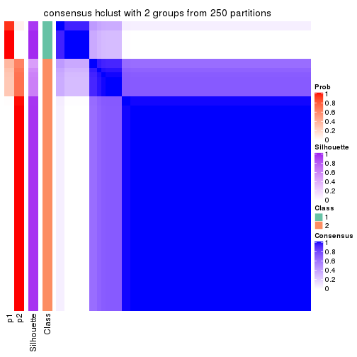
consensus_heatmap(res, k = 3)
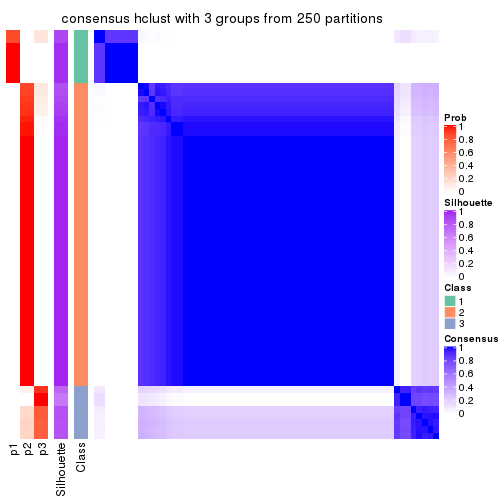
consensus_heatmap(res, k = 4)
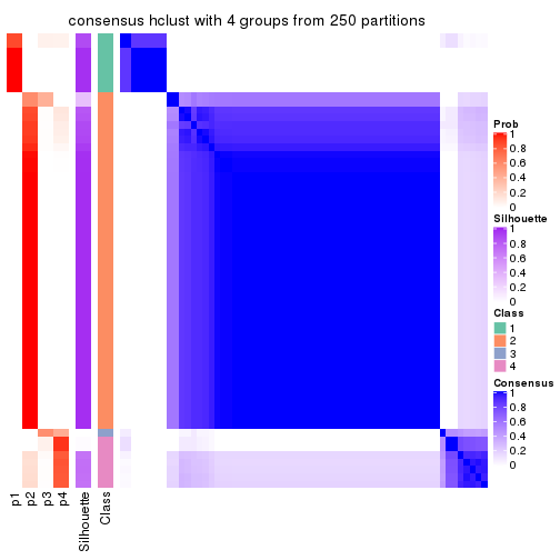
consensus_heatmap(res, k = 5)
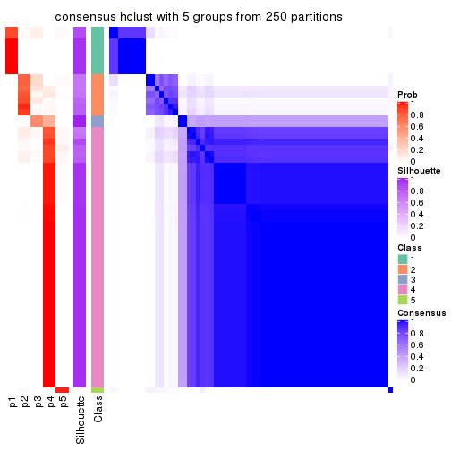
consensus_heatmap(res, k = 6)
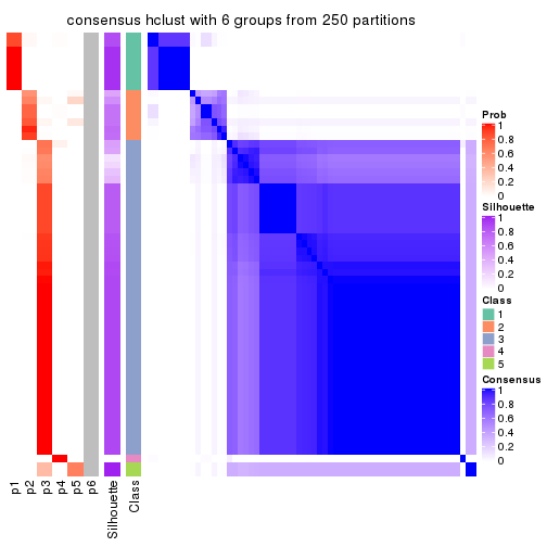
Heatmaps for the membership of samples in all partitions to see how consistent they are:
membership_heatmap(res, k = 2)
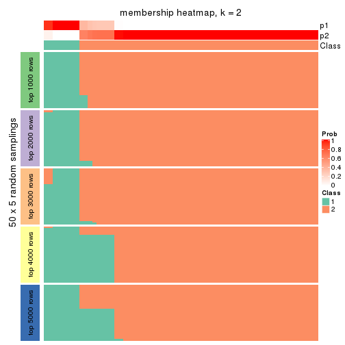
membership_heatmap(res, k = 3)
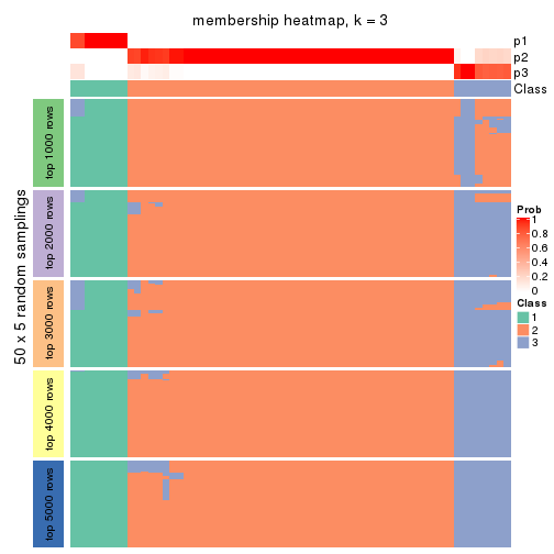
membership_heatmap(res, k = 4)
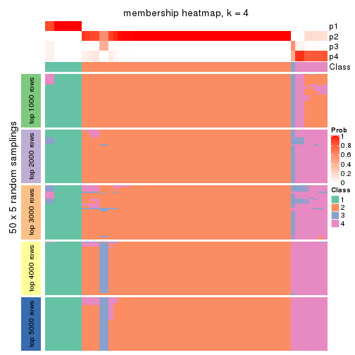
membership_heatmap(res, k = 5)
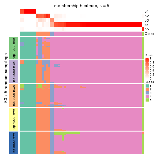
membership_heatmap(res, k = 6)
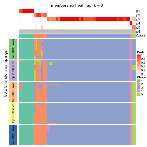
As soon as we have had the classes for columns, we can look for signatures which are significantly different between classes which can be candidate marks for certain classes. Following are the heatmaps for signatures.
Signature heatmaps where rows are scaled:
get_signatures(res, k = 2)
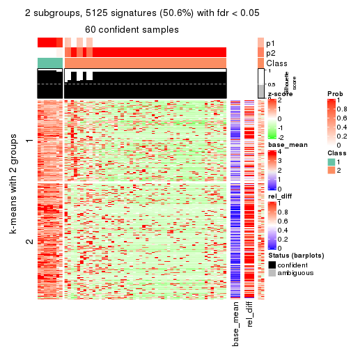
get_signatures(res, k = 3)
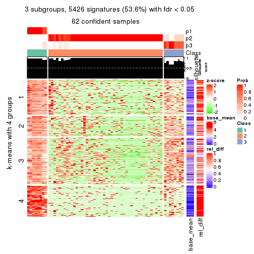
get_signatures(res, k = 4)
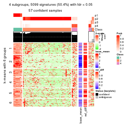
get_signatures(res, k = 5)
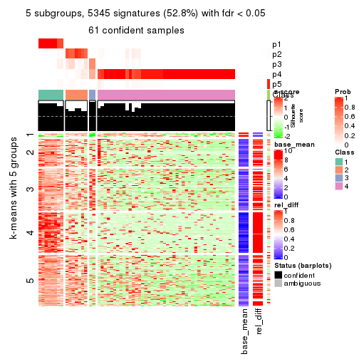
get_signatures(res, k = 6)
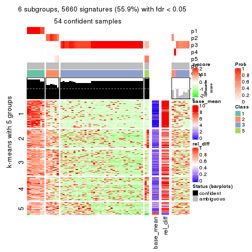
Signature heatmaps where rows are not scaled:
get_signatures(res, k = 2, scale_rows = FALSE)
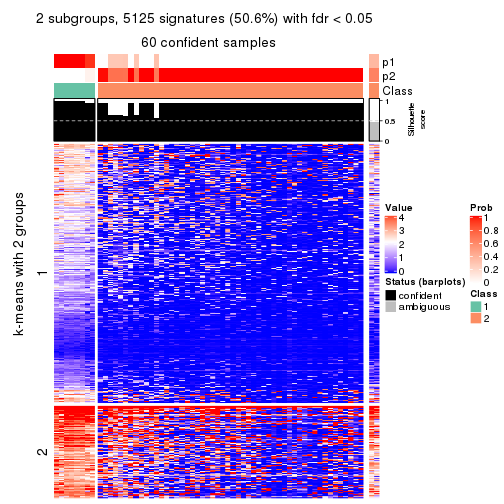
get_signatures(res, k = 3, scale_rows = FALSE)
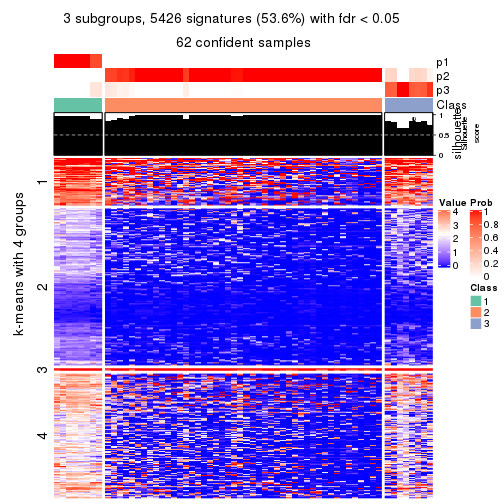
get_signatures(res, k = 4, scale_rows = FALSE)
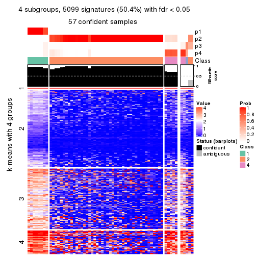
get_signatures(res, k = 5, scale_rows = FALSE)
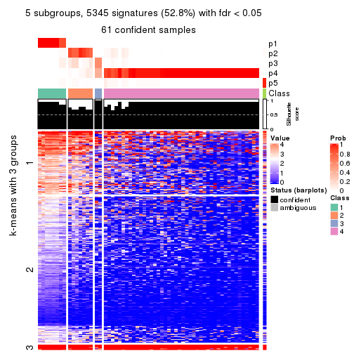
get_signatures(res, k = 6, scale_rows = FALSE)
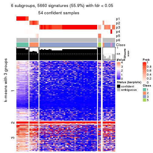
Compare the overlap of signatures from different k:
compare_signatures(res)
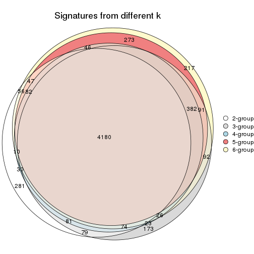
get_signature() returns a data frame invisibly. TO get the list of signatures, the function
call should be assigned to a variable explicitly. In following code, if plot argument is set
to FALSE, no heatmap is plotted while only the differential analysis is performed.
# code only for demonstration
tb = get_signature(res, k = ..., plot = FALSE)
An example of the output of tb is:
#> which_row fdr mean_1 mean_2 scaled_mean_1 scaled_mean_2 km
#> 1 38 0.042760348 8.373488 9.131774 -0.5533452 0.5164555 1
#> 2 40 0.018707592 7.106213 8.469186 -0.6173731 0.5762149 1
#> 3 55 0.019134737 10.221463 11.207825 -0.6159697 0.5749050 1
#> 4 59 0.006059896 5.921854 7.869574 -0.6899429 0.6439467 1
#> 5 60 0.018055526 8.928898 10.211722 -0.6204761 0.5791110 1
#> 6 98 0.009384629 15.714769 14.887706 0.6635654 -0.6193277 2
...
The columns in tb are:
which_row: row indices corresponding to the input matrix.fdr: FDR for the differential test. mean_x: The mean value in group x.scaled_mean_x: The mean value in group x after rows are scaled.km: Row groups if k-means clustering is applied to rows.UMAP plot which shows how samples are separated.
dimension_reduction(res, k = 2, method = "UMAP")

dimension_reduction(res, k = 3, method = "UMAP")
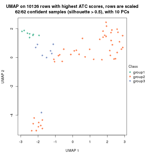
dimension_reduction(res, k = 4, method = "UMAP")
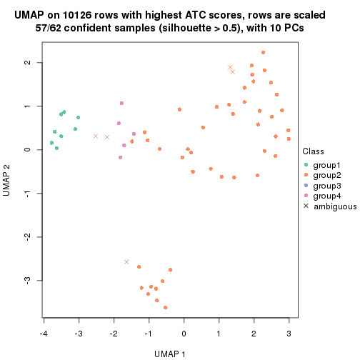
dimension_reduction(res, k = 5, method = "UMAP")
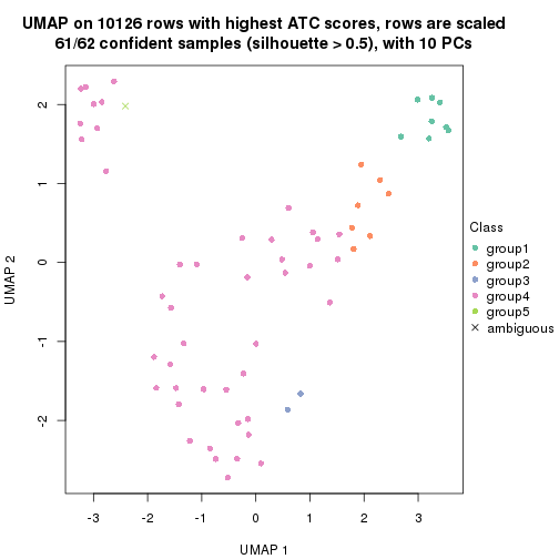
dimension_reduction(res, k = 6, method = "UMAP")
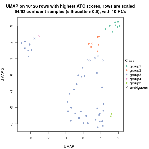
Following heatmap shows how subgroups are split when increasing k:
collect_classes(res)
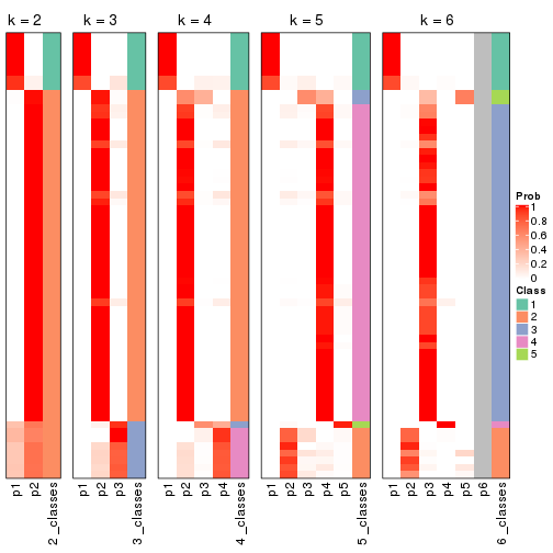
If matrix rows can be associated to genes, consider to use functional_enrichment(res,
...) to perform function enrichment for the signature genes. See this vignette for more detailed explanations.
The object with results only for a single top-value method and a single partition method can be extracted as:
res = res_list["ATC", "kmeans"]
# you can also extract it by
# res = res_list["ATC:kmeans"]
A summary of res and all the functions that can be applied to it:
res
#> A 'ConsensusPartition' object with k = 2, 3, 4, 5, 6.
#> On a matrix with 10126 rows and 62 columns.
#> Top rows (1000, 2000, 3000, 4000, 5000) are extracted by 'ATC' method.
#> Subgroups are detected by 'kmeans' method.
#> Performed in total 1250 partitions by row resampling.
#> Best k for subgroups seems to be 2.
#>
#> Following methods can be applied to this 'ConsensusPartition' object:
#> [1] "cola_report" "collect_classes" "collect_plots"
#> [4] "collect_stats" "colnames" "compare_signatures"
#> [7] "consensus_heatmap" "dimension_reduction" "functional_enrichment"
#> [10] "get_anno_col" "get_anno" "get_classes"
#> [13] "get_consensus" "get_matrix" "get_membership"
#> [16] "get_param" "get_signatures" "get_stats"
#> [19] "is_best_k" "is_stable_k" "membership_heatmap"
#> [22] "ncol" "nrow" "plot_ecdf"
#> [25] "rownames" "select_partition_number" "show"
#> [28] "suggest_best_k" "test_to_known_factors"
collect_plots() function collects all the plots made from res for all k (number of partitions)
into one single page to provide an easy and fast comparison between different k.
collect_plots(res)
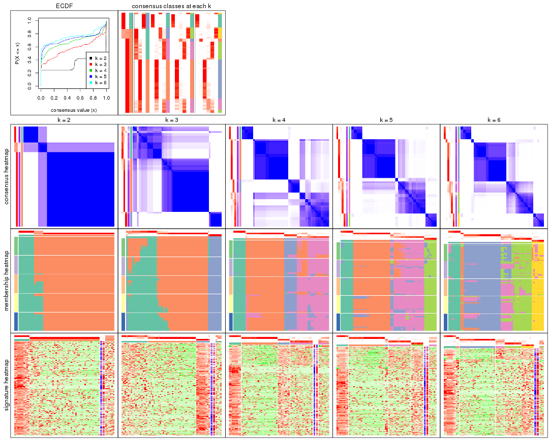
The plots are:
k and the heatmap of
predicted classes for each k.k.k.k.All the plots in panels can be made by individual functions and they are plotted later in this section.
select_partition_number() produces several plots showing different
statistics for choosing “optimized” k. There are following statistics:
k;k, the area increased is defined as \(A_k - A_{k-1}\).The detailed explanations of these statistics can be found in the cola vignette.
Generally speaking, lower PAC score, higher mean silhouette score or higher
concordance corresponds to better partition. Rand index and Jaccard index
measure how similar the current partition is compared to partition with k-1.
If they are too similar, we won't accept k is better than k-1.
select_partition_number(res)
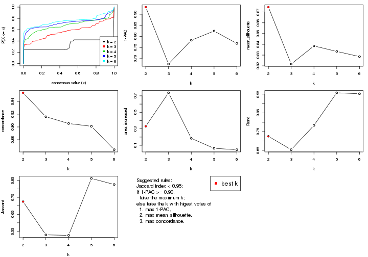
The numeric values for all these statistics can be obtained by get_stats().
get_stats(res)
#> k 1-PAC mean_silhouette concordance area_increased Rand Jaccard
#> 2 2 0.932 0.875 0.953 0.3307 0.725 0.725
#> 3 3 0.676 0.822 0.916 0.7367 0.654 0.529
#> 4 4 0.783 0.838 0.905 0.1845 0.783 0.526
#> 5 5 0.825 0.833 0.901 0.0633 0.957 0.862
#> 6 6 0.768 0.829 0.864 0.0472 0.952 0.826
suggest_best_k() suggests the best \(k\) based on these statistics. The rules are as follows:
suggest_best_k(res)
#> [1] 2
Following shows the table of the partitions (You need to click the show/hide
code output link to see it). The membership matrix (columns with name p*)
is inferred by
clue::cl_consensus()
function with the SE method. Basically the value in the membership matrix
represents the probability to belong to a certain group. The finall class
label for an item is determined with the group with highest probability it
belongs to.
In get_classes() function, the entropy is calculated from the membership
matrix and the silhouette score is calculated from the consensus matrix.
cbind(get_classes(res, k = 2), get_membership(res, k = 2))
#> class entropy silhouette p1 p2
#> SRR764776 1 0.000 1.000 1.000 0.000
#> SRR764777 1 0.000 1.000 1.000 0.000
#> SRR764778 1 0.000 1.000 1.000 0.000
#> SRR764779 1 0.000 1.000 1.000 0.000
#> SRR764780 1 0.000 1.000 1.000 0.000
#> SRR764781 1 0.000 1.000 1.000 0.000
#> SRR764782 2 0.000 0.941 0.000 1.000
#> SRR764783 2 1.000 0.141 0.488 0.512
#> SRR764784 2 0.000 0.941 0.000 1.000
#> SRR764785 2 0.000 0.941 0.000 1.000
#> SRR764786 2 0.000 0.941 0.000 1.000
#> SRR764787 2 0.000 0.941 0.000 1.000
#> SRR764788 2 0.000 0.941 0.000 1.000
#> SRR764789 2 0.000 0.941 0.000 1.000
#> SRR764790 2 0.000 0.941 0.000 1.000
#> SRR764791 2 0.000 0.941 0.000 1.000
#> SRR764792 2 0.000 0.941 0.000 1.000
#> SRR764793 2 0.000 0.941 0.000 1.000
#> SRR764794 2 0.000 0.941 0.000 1.000
#> SRR764795 2 0.000 0.941 0.000 1.000
#> SRR764796 2 0.000 0.941 0.000 1.000
#> SRR764797 2 0.999 0.153 0.484 0.516
#> SRR764798 2 0.000 0.941 0.000 1.000
#> SRR764799 1 0.000 1.000 1.000 0.000
#> SRR764800 1 0.000 1.000 1.000 0.000
#> SRR764801 2 0.000 0.941 0.000 1.000
#> SRR764802 2 0.993 0.242 0.452 0.548
#> SRR764803 2 1.000 0.141 0.488 0.512
#> SRR764804 2 0.000 0.941 0.000 1.000
#> SRR764805 2 0.000 0.941 0.000 1.000
#> SRR764806 2 0.000 0.941 0.000 1.000
#> SRR764807 2 0.000 0.941 0.000 1.000
#> SRR764808 2 0.000 0.941 0.000 1.000
#> SRR764809 2 0.000 0.941 0.000 1.000
#> SRR764810 2 0.000 0.941 0.000 1.000
#> SRR764811 2 0.000 0.941 0.000 1.000
#> SRR764812 2 0.000 0.941 0.000 1.000
#> SRR764813 2 0.000 0.941 0.000 1.000
#> SRR764814 2 1.000 0.141 0.488 0.512
#> SRR764815 2 0.000 0.941 0.000 1.000
#> SRR764816 1 0.000 1.000 1.000 0.000
#> SRR764817 1 0.000 1.000 1.000 0.000
#> SRR1066622 2 0.000 0.941 0.000 1.000
#> SRR1066623 2 0.000 0.941 0.000 1.000
#> SRR1066624 2 1.000 0.141 0.488 0.512
#> SRR1066625 2 0.000 0.941 0.000 1.000
#> SRR1066626 2 0.000 0.941 0.000 1.000
#> SRR1066627 2 0.000 0.941 0.000 1.000
#> SRR1066628 2 0.000 0.941 0.000 1.000
#> SRR1066629 2 0.000 0.941 0.000 1.000
#> SRR1066630 2 0.000 0.941 0.000 1.000
#> SRR1066631 2 0.000 0.941 0.000 1.000
#> SRR1066632 2 0.000 0.941 0.000 1.000
#> SRR1066633 2 0.000 0.941 0.000 1.000
#> SRR1066634 2 0.000 0.941 0.000 1.000
#> SRR1066635 2 0.000 0.941 0.000 1.000
#> SRR1066636 2 0.000 0.941 0.000 1.000
#> SRR1066637 2 0.000 0.941 0.000 1.000
#> SRR1066638 2 0.000 0.941 0.000 1.000
#> SRR1066639 2 0.000 0.941 0.000 1.000
#> SRR1066640 2 0.000 0.941 0.000 1.000
#> SRR1066641 2 0.000 0.941 0.000 1.000
cbind(get_classes(res, k = 3), get_membership(res, k = 3))
#> class entropy silhouette p1 p2 p3
#> SRR764776 3 0.0000 0.9712 0.000 0.000 1.000
#> SRR764777 3 0.0000 0.9712 0.000 0.000 1.000
#> SRR764778 3 0.0000 0.9712 0.000 0.000 1.000
#> SRR764779 3 0.0000 0.9712 0.000 0.000 1.000
#> SRR764780 3 0.5178 0.7329 0.256 0.000 0.744
#> SRR764781 1 0.5988 0.0677 0.632 0.000 0.368
#> SRR764782 1 0.3686 0.7874 0.860 0.140 0.000
#> SRR764783 1 0.0237 0.7463 0.996 0.004 0.000
#> SRR764784 1 0.5138 0.7395 0.748 0.252 0.000
#> SRR764785 2 0.0000 0.9387 0.000 1.000 0.000
#> SRR764786 2 0.0000 0.9387 0.000 1.000 0.000
#> SRR764787 1 0.6225 0.4121 0.568 0.432 0.000
#> SRR764788 1 0.2448 0.7843 0.924 0.076 0.000
#> SRR764789 2 0.4702 0.6990 0.212 0.788 0.000
#> SRR764790 2 0.0000 0.9387 0.000 1.000 0.000
#> SRR764791 2 0.6026 0.2779 0.376 0.624 0.000
#> SRR764792 1 0.5988 0.5620 0.632 0.368 0.000
#> SRR764793 1 0.5138 0.7395 0.748 0.252 0.000
#> SRR764794 1 0.6305 0.2474 0.516 0.484 0.000
#> SRR764795 1 0.2878 0.7902 0.904 0.096 0.000
#> SRR764796 1 0.5178 0.7355 0.744 0.256 0.000
#> SRR764797 1 0.0237 0.7463 0.996 0.004 0.000
#> SRR764798 1 0.2711 0.7885 0.912 0.088 0.000
#> SRR764799 3 0.0237 0.9699 0.004 0.000 0.996
#> SRR764800 3 0.0237 0.9699 0.004 0.000 0.996
#> SRR764801 1 0.2878 0.7902 0.904 0.096 0.000
#> SRR764802 1 0.0237 0.7463 0.996 0.004 0.000
#> SRR764803 1 0.0237 0.7463 0.996 0.004 0.000
#> SRR764804 2 0.0000 0.9387 0.000 1.000 0.000
#> SRR764805 2 0.0000 0.9387 0.000 1.000 0.000
#> SRR764806 2 0.0000 0.9387 0.000 1.000 0.000
#> SRR764807 2 0.0000 0.9387 0.000 1.000 0.000
#> SRR764808 2 0.0000 0.9387 0.000 1.000 0.000
#> SRR764809 2 0.0000 0.9387 0.000 1.000 0.000
#> SRR764810 2 0.0000 0.9387 0.000 1.000 0.000
#> SRR764811 2 0.0000 0.9387 0.000 1.000 0.000
#> SRR764812 2 0.0000 0.9387 0.000 1.000 0.000
#> SRR764813 2 0.0000 0.9387 0.000 1.000 0.000
#> SRR764814 1 0.0237 0.7463 0.996 0.004 0.000
#> SRR764815 1 0.5431 0.7014 0.716 0.284 0.000
#> SRR764816 3 0.0000 0.9712 0.000 0.000 1.000
#> SRR764817 3 0.0000 0.9712 0.000 0.000 1.000
#> SRR1066622 2 0.4062 0.7725 0.164 0.836 0.000
#> SRR1066623 2 0.4062 0.7725 0.164 0.836 0.000
#> SRR1066624 1 0.0237 0.7463 0.996 0.004 0.000
#> SRR1066625 1 0.4452 0.7758 0.808 0.192 0.000
#> SRR1066626 2 0.0000 0.9387 0.000 1.000 0.000
#> SRR1066627 2 0.5138 0.6219 0.252 0.748 0.000
#> SRR1066628 2 0.3340 0.8263 0.120 0.880 0.000
#> SRR1066629 2 0.4702 0.6990 0.212 0.788 0.000
#> SRR1066630 2 0.0000 0.9387 0.000 1.000 0.000
#> SRR1066631 2 0.1411 0.9097 0.036 0.964 0.000
#> SRR1066632 2 0.0000 0.9387 0.000 1.000 0.000
#> SRR1066633 2 0.0000 0.9387 0.000 1.000 0.000
#> SRR1066634 2 0.0000 0.9387 0.000 1.000 0.000
#> SRR1066635 2 0.0000 0.9387 0.000 1.000 0.000
#> SRR1066636 2 0.0000 0.9387 0.000 1.000 0.000
#> SRR1066637 2 0.0000 0.9387 0.000 1.000 0.000
#> SRR1066638 2 0.0000 0.9387 0.000 1.000 0.000
#> SRR1066639 2 0.0000 0.9387 0.000 1.000 0.000
#> SRR1066640 2 0.0000 0.9387 0.000 1.000 0.000
#> SRR1066641 2 0.0000 0.9387 0.000 1.000 0.000
cbind(get_classes(res, k = 4), get_membership(res, k = 4))
#> class entropy silhouette p1 p2 p3 p4
#> SRR764776 1 0.0000 0.988 1.000 0.000 0.000 0.000
#> SRR764777 1 0.0000 0.988 1.000 0.000 0.000 0.000
#> SRR764778 1 0.0000 0.988 1.000 0.000 0.000 0.000
#> SRR764779 1 0.0000 0.988 1.000 0.000 0.000 0.000
#> SRR764780 3 0.2149 0.852 0.088 0.000 0.912 0.000
#> SRR764781 3 0.2224 0.916 0.032 0.000 0.928 0.040
#> SRR764782 4 0.1520 0.737 0.000 0.020 0.024 0.956
#> SRR764783 3 0.2647 0.964 0.000 0.000 0.880 0.120
#> SRR764784 4 0.2335 0.770 0.000 0.060 0.020 0.920
#> SRR764785 2 0.0592 0.951 0.000 0.984 0.000 0.016
#> SRR764786 2 0.0000 0.955 0.000 1.000 0.000 0.000
#> SRR764787 4 0.2149 0.781 0.000 0.088 0.000 0.912
#> SRR764788 4 0.2868 0.628 0.000 0.000 0.136 0.864
#> SRR764789 4 0.3610 0.748 0.000 0.200 0.000 0.800
#> SRR764790 2 0.0000 0.955 0.000 1.000 0.000 0.000
#> SRR764791 4 0.2760 0.774 0.000 0.128 0.000 0.872
#> SRR764792 4 0.2011 0.780 0.000 0.080 0.000 0.920
#> SRR764793 4 0.1902 0.776 0.000 0.064 0.004 0.932
#> SRR764794 4 0.2345 0.780 0.000 0.100 0.000 0.900
#> SRR764795 4 0.2773 0.651 0.000 0.004 0.116 0.880
#> SRR764796 4 0.2335 0.770 0.000 0.060 0.020 0.920
#> SRR764797 3 0.2647 0.964 0.000 0.000 0.880 0.120
#> SRR764798 4 0.4509 0.458 0.000 0.004 0.288 0.708
#> SRR764799 1 0.0657 0.983 0.984 0.000 0.012 0.004
#> SRR764800 1 0.0657 0.983 0.984 0.000 0.012 0.004
#> SRR764801 4 0.4456 0.474 0.000 0.004 0.280 0.716
#> SRR764802 3 0.2647 0.964 0.000 0.000 0.880 0.120
#> SRR764803 3 0.2647 0.964 0.000 0.000 0.880 0.120
#> SRR764804 2 0.0000 0.955 0.000 1.000 0.000 0.000
#> SRR764805 2 0.0000 0.955 0.000 1.000 0.000 0.000
#> SRR764806 2 0.1637 0.932 0.000 0.940 0.000 0.060
#> SRR764807 2 0.0000 0.955 0.000 1.000 0.000 0.000
#> SRR764808 2 0.0000 0.955 0.000 1.000 0.000 0.000
#> SRR764809 2 0.0000 0.955 0.000 1.000 0.000 0.000
#> SRR764810 2 0.0000 0.955 0.000 1.000 0.000 0.000
#> SRR764811 2 0.0000 0.955 0.000 1.000 0.000 0.000
#> SRR764812 2 0.0000 0.955 0.000 1.000 0.000 0.000
#> SRR764813 2 0.0000 0.955 0.000 1.000 0.000 0.000
#> SRR764814 3 0.2589 0.963 0.000 0.000 0.884 0.116
#> SRR764815 4 0.1637 0.776 0.000 0.060 0.000 0.940
#> SRR764816 1 0.1118 0.973 0.964 0.000 0.036 0.000
#> SRR764817 1 0.1118 0.973 0.964 0.000 0.036 0.000
#> SRR1066622 4 0.4925 0.427 0.000 0.428 0.000 0.572
#> SRR1066623 4 0.4916 0.436 0.000 0.424 0.000 0.576
#> SRR1066624 3 0.2469 0.959 0.000 0.000 0.892 0.108
#> SRR1066625 4 0.1151 0.727 0.000 0.008 0.024 0.968
#> SRR1066626 2 0.4830 0.183 0.000 0.608 0.000 0.392
#> SRR1066627 4 0.3688 0.744 0.000 0.208 0.000 0.792
#> SRR1066628 4 0.4948 0.398 0.000 0.440 0.000 0.560
#> SRR1066629 4 0.4222 0.685 0.000 0.272 0.000 0.728
#> SRR1066630 2 0.0000 0.955 0.000 1.000 0.000 0.000
#> SRR1066631 4 0.4977 0.341 0.000 0.460 0.000 0.540
#> SRR1066632 2 0.1637 0.932 0.000 0.940 0.000 0.060
#> SRR1066633 2 0.1637 0.932 0.000 0.940 0.000 0.060
#> SRR1066634 2 0.1637 0.932 0.000 0.940 0.000 0.060
#> SRR1066635 2 0.0000 0.955 0.000 1.000 0.000 0.000
#> SRR1066636 2 0.1211 0.942 0.000 0.960 0.000 0.040
#> SRR1066637 2 0.1637 0.932 0.000 0.940 0.000 0.060
#> SRR1066638 2 0.1637 0.932 0.000 0.940 0.000 0.060
#> SRR1066639 2 0.0817 0.948 0.000 0.976 0.000 0.024
#> SRR1066640 2 0.1637 0.932 0.000 0.940 0.000 0.060
#> SRR1066641 2 0.0000 0.955 0.000 1.000 0.000 0.000
cbind(get_classes(res, k = 5), get_membership(res, k = 5))
#> class entropy silhouette p1 p2 p3 p4 p5
#> SRR764776 1 0.0000 0.957 1.000 0.000 0.000 0.000 0.000
#> SRR764777 1 0.0000 0.957 1.000 0.000 0.000 0.000 0.000
#> SRR764778 1 0.0000 0.957 1.000 0.000 0.000 0.000 0.000
#> SRR764779 1 0.0000 0.957 1.000 0.000 0.000 0.000 0.000
#> SRR764780 5 0.2624 0.869 0.012 0.000 0.116 0.000 0.872
#> SRR764781 5 0.2389 0.876 0.004 0.000 0.116 0.000 0.880
#> SRR764782 4 0.1830 0.661 0.000 0.004 0.052 0.932 0.012
#> SRR764783 5 0.0510 0.936 0.000 0.000 0.000 0.016 0.984
#> SRR764784 4 0.1605 0.684 0.000 0.012 0.040 0.944 0.004
#> SRR764785 2 0.0898 0.955 0.000 0.972 0.020 0.008 0.000
#> SRR764786 2 0.0000 0.960 0.000 1.000 0.000 0.000 0.000
#> SRR764787 4 0.1195 0.699 0.000 0.012 0.028 0.960 0.000
#> SRR764788 4 0.2922 0.580 0.000 0.000 0.056 0.872 0.072
#> SRR764789 4 0.3043 0.679 0.000 0.056 0.080 0.864 0.000
#> SRR764790 2 0.0000 0.960 0.000 1.000 0.000 0.000 0.000
#> SRR764791 4 0.1469 0.699 0.000 0.016 0.036 0.948 0.000
#> SRR764792 4 0.1444 0.689 0.000 0.012 0.040 0.948 0.000
#> SRR764793 4 0.1444 0.688 0.000 0.012 0.040 0.948 0.000
#> SRR764794 4 0.1106 0.694 0.000 0.012 0.024 0.964 0.000
#> SRR764795 4 0.2726 0.596 0.000 0.000 0.052 0.884 0.064
#> SRR764796 4 0.1525 0.691 0.000 0.012 0.036 0.948 0.004
#> SRR764797 5 0.1300 0.932 0.000 0.000 0.028 0.016 0.956
#> SRR764798 3 0.4967 1.000 0.000 0.000 0.660 0.280 0.060
#> SRR764799 1 0.1282 0.943 0.952 0.000 0.044 0.000 0.004
#> SRR764800 1 0.1282 0.943 0.952 0.000 0.044 0.000 0.004
#> SRR764801 3 0.4967 1.000 0.000 0.000 0.660 0.280 0.060
#> SRR764802 5 0.0671 0.936 0.000 0.000 0.004 0.016 0.980
#> SRR764803 5 0.2110 0.897 0.000 0.000 0.072 0.016 0.912
#> SRR764804 2 0.0000 0.960 0.000 1.000 0.000 0.000 0.000
#> SRR764805 2 0.0000 0.960 0.000 1.000 0.000 0.000 0.000
#> SRR764806 2 0.2331 0.934 0.000 0.900 0.080 0.020 0.000
#> SRR764807 2 0.0000 0.960 0.000 1.000 0.000 0.000 0.000
#> SRR764808 2 0.0000 0.960 0.000 1.000 0.000 0.000 0.000
#> SRR764809 2 0.0000 0.960 0.000 1.000 0.000 0.000 0.000
#> SRR764810 2 0.0000 0.960 0.000 1.000 0.000 0.000 0.000
#> SRR764811 2 0.0000 0.960 0.000 1.000 0.000 0.000 0.000
#> SRR764812 2 0.0000 0.960 0.000 1.000 0.000 0.000 0.000
#> SRR764813 2 0.0000 0.960 0.000 1.000 0.000 0.000 0.000
#> SRR764814 5 0.0671 0.936 0.000 0.000 0.004 0.016 0.980
#> SRR764815 4 0.1106 0.694 0.000 0.012 0.024 0.964 0.000
#> SRR764816 1 0.2470 0.900 0.884 0.000 0.104 0.000 0.012
#> SRR764817 1 0.2470 0.900 0.884 0.000 0.104 0.000 0.012
#> SRR1066622 4 0.5739 0.484 0.000 0.280 0.124 0.596 0.000
#> SRR1066623 4 0.5681 0.496 0.000 0.268 0.124 0.608 0.000
#> SRR1066624 5 0.1831 0.915 0.000 0.000 0.076 0.004 0.920
#> SRR1066625 4 0.2280 0.661 0.000 0.000 0.120 0.880 0.000
#> SRR1066626 4 0.6100 0.284 0.000 0.428 0.124 0.448 0.000
#> SRR1066627 4 0.3861 0.652 0.000 0.068 0.128 0.804 0.000
#> SRR1066628 4 0.5941 0.429 0.000 0.332 0.124 0.544 0.000
#> SRR1066629 4 0.4548 0.617 0.000 0.124 0.124 0.752 0.000
#> SRR1066630 2 0.0000 0.960 0.000 1.000 0.000 0.000 0.000
#> SRR1066631 4 0.6024 0.389 0.000 0.364 0.124 0.512 0.000
#> SRR1066632 2 0.2331 0.934 0.000 0.900 0.080 0.020 0.000
#> SRR1066633 2 0.2654 0.921 0.000 0.884 0.084 0.032 0.000
#> SRR1066634 2 0.2331 0.934 0.000 0.900 0.080 0.020 0.000
#> SRR1066635 2 0.0794 0.955 0.000 0.972 0.028 0.000 0.000
#> SRR1066636 2 0.2110 0.939 0.000 0.912 0.072 0.016 0.000
#> SRR1066637 2 0.2331 0.934 0.000 0.900 0.080 0.020 0.000
#> SRR1066638 2 0.2331 0.934 0.000 0.900 0.080 0.020 0.000
#> SRR1066639 2 0.1894 0.942 0.000 0.920 0.072 0.008 0.000
#> SRR1066640 2 0.2331 0.934 0.000 0.900 0.080 0.020 0.000
#> SRR1066641 2 0.0000 0.960 0.000 1.000 0.000 0.000 0.000
cbind(get_classes(res, k = 6), get_membership(res, k = 6))
#> class entropy silhouette p1 p2 p3 p4 p5 p6
#> SRR764776 1 0.0000 0.939 1.000 0.000 0.000 0.000 0.000 0.000
#> SRR764777 1 0.0000 0.939 1.000 0.000 0.000 0.000 0.000 0.000
#> SRR764778 1 0.0000 0.939 1.000 0.000 0.000 0.000 0.000 0.000
#> SRR764779 1 0.0000 0.939 1.000 0.000 0.000 0.000 0.000 0.000
#> SRR764780 6 0.2882 0.829 0.000 0.008 0.000 0.180 0.000 0.812
#> SRR764781 6 0.2882 0.829 0.000 0.008 0.000 0.180 0.000 0.812
#> SRR764782 5 0.0820 0.830 0.000 0.016 0.000 0.012 0.972 0.000
#> SRR764783 6 0.0260 0.892 0.000 0.000 0.000 0.008 0.000 0.992
#> SRR764784 5 0.0260 0.838 0.000 0.000 0.000 0.008 0.992 0.000
#> SRR764785 3 0.1760 0.887 0.000 0.020 0.928 0.048 0.004 0.000
#> SRR764786 3 0.0000 0.901 0.000 0.000 1.000 0.000 0.000 0.000
#> SRR764787 5 0.2219 0.790 0.000 0.000 0.000 0.136 0.864 0.000
#> SRR764788 5 0.1542 0.812 0.000 0.016 0.000 0.016 0.944 0.024
#> SRR764789 5 0.4247 0.419 0.000 0.000 0.040 0.296 0.664 0.000
#> SRR764790 3 0.0000 0.901 0.000 0.000 1.000 0.000 0.000 0.000
#> SRR764791 5 0.2964 0.713 0.000 0.004 0.000 0.204 0.792 0.000
#> SRR764792 5 0.1082 0.844 0.000 0.004 0.000 0.040 0.956 0.000
#> SRR764793 5 0.0692 0.842 0.000 0.004 0.000 0.020 0.976 0.000
#> SRR764794 5 0.1700 0.834 0.000 0.004 0.000 0.080 0.916 0.000
#> SRR764795 5 0.1542 0.812 0.000 0.016 0.000 0.016 0.944 0.024
#> SRR764796 5 0.1152 0.841 0.000 0.004 0.000 0.044 0.952 0.000
#> SRR764797 6 0.1418 0.883 0.000 0.024 0.000 0.032 0.000 0.944
#> SRR764798 2 0.1866 1.000 0.000 0.908 0.000 0.000 0.084 0.008
#> SRR764799 1 0.1549 0.919 0.936 0.020 0.000 0.044 0.000 0.000
#> SRR764800 1 0.1549 0.919 0.936 0.020 0.000 0.044 0.000 0.000
#> SRR764801 2 0.1866 1.000 0.000 0.908 0.000 0.000 0.084 0.008
#> SRR764802 6 0.0146 0.892 0.000 0.000 0.000 0.004 0.000 0.996
#> SRR764803 6 0.2744 0.827 0.000 0.144 0.000 0.016 0.000 0.840
#> SRR764804 3 0.0000 0.901 0.000 0.000 1.000 0.000 0.000 0.000
#> SRR764805 3 0.0000 0.901 0.000 0.000 1.000 0.000 0.000 0.000
#> SRR764806 3 0.3567 0.833 0.000 0.052 0.804 0.136 0.008 0.000
#> SRR764807 3 0.0000 0.901 0.000 0.000 1.000 0.000 0.000 0.000
#> SRR764808 3 0.0000 0.901 0.000 0.000 1.000 0.000 0.000 0.000
#> SRR764809 3 0.0000 0.901 0.000 0.000 1.000 0.000 0.000 0.000
#> SRR764810 3 0.0000 0.901 0.000 0.000 1.000 0.000 0.000 0.000
#> SRR764811 3 0.0000 0.901 0.000 0.000 1.000 0.000 0.000 0.000
#> SRR764812 3 0.0000 0.901 0.000 0.000 1.000 0.000 0.000 0.000
#> SRR764813 3 0.0000 0.901 0.000 0.000 1.000 0.000 0.000 0.000
#> SRR764814 6 0.0603 0.891 0.000 0.004 0.000 0.016 0.000 0.980
#> SRR764815 5 0.1556 0.830 0.000 0.000 0.000 0.080 0.920 0.000
#> SRR764816 1 0.2482 0.857 0.848 0.004 0.000 0.148 0.000 0.000
#> SRR764817 1 0.2482 0.857 0.848 0.004 0.000 0.148 0.000 0.000
#> SRR1066622 4 0.5575 0.765 0.000 0.000 0.200 0.548 0.252 0.000
#> SRR1066623 4 0.5565 0.773 0.000 0.000 0.208 0.552 0.240 0.000
#> SRR1066624 6 0.3422 0.792 0.000 0.036 0.000 0.176 0.000 0.788
#> SRR1066625 5 0.4076 0.136 0.000 0.008 0.000 0.452 0.540 0.000
#> SRR1066626 4 0.5480 0.728 0.000 0.000 0.328 0.528 0.144 0.000
#> SRR1066627 4 0.4709 0.393 0.000 0.004 0.040 0.556 0.400 0.000
#> SRR1066628 4 0.5602 0.775 0.000 0.000 0.276 0.536 0.188 0.000
#> SRR1066629 4 0.5135 0.536 0.000 0.004 0.080 0.552 0.364 0.000
#> SRR1066630 3 0.0000 0.901 0.000 0.000 1.000 0.000 0.000 0.000
#> SRR1066631 4 0.5561 0.755 0.000 0.000 0.308 0.528 0.164 0.000
#> SRR1066632 3 0.3567 0.833 0.000 0.052 0.804 0.136 0.008 0.000
#> SRR1066633 3 0.3928 0.781 0.000 0.052 0.764 0.176 0.008 0.000
#> SRR1066634 3 0.3567 0.833 0.000 0.052 0.804 0.136 0.008 0.000
#> SRR1066635 3 0.1863 0.884 0.000 0.044 0.920 0.036 0.000 0.000
#> SRR1066636 3 0.3376 0.841 0.000 0.052 0.816 0.128 0.004 0.000
#> SRR1066637 3 0.3567 0.833 0.000 0.052 0.804 0.136 0.008 0.000
#> SRR1066638 3 0.3567 0.833 0.000 0.052 0.804 0.136 0.008 0.000
#> SRR1066639 3 0.3112 0.854 0.000 0.052 0.840 0.104 0.004 0.000
#> SRR1066640 3 0.3567 0.833 0.000 0.052 0.804 0.136 0.008 0.000
#> SRR1066641 3 0.0000 0.901 0.000 0.000 1.000 0.000 0.000 0.000
Heatmaps for the consensus matrix. It visualizes the probability of two samples to be in a same group.
consensus_heatmap(res, k = 2)
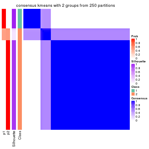
consensus_heatmap(res, k = 3)
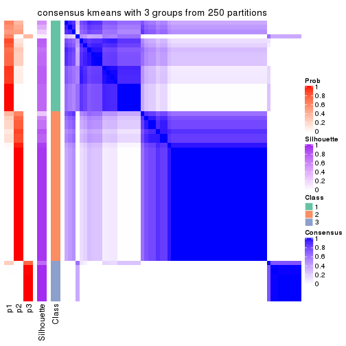
consensus_heatmap(res, k = 4)
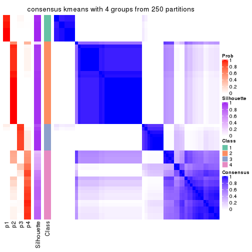
consensus_heatmap(res, k = 5)

consensus_heatmap(res, k = 6)
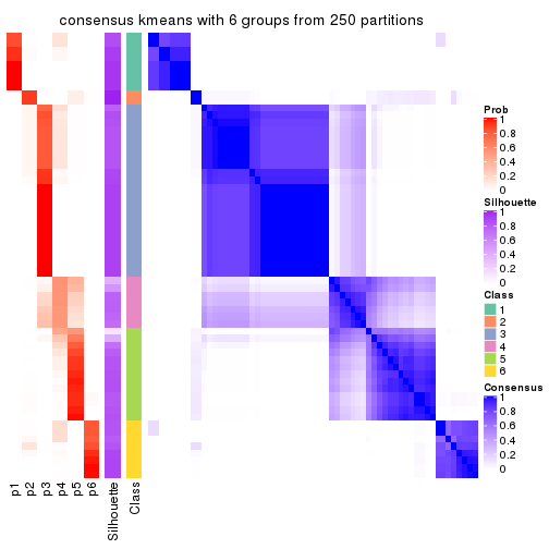
Heatmaps for the membership of samples in all partitions to see how consistent they are:
membership_heatmap(res, k = 2)
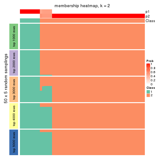
membership_heatmap(res, k = 3)
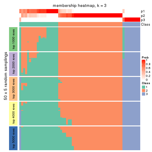
membership_heatmap(res, k = 4)
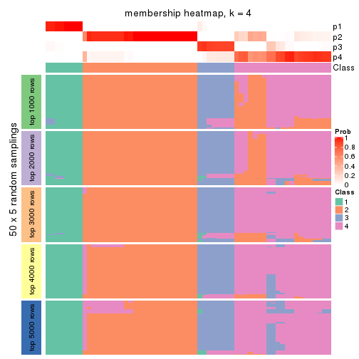
membership_heatmap(res, k = 5)
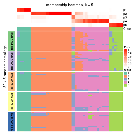
membership_heatmap(res, k = 6)
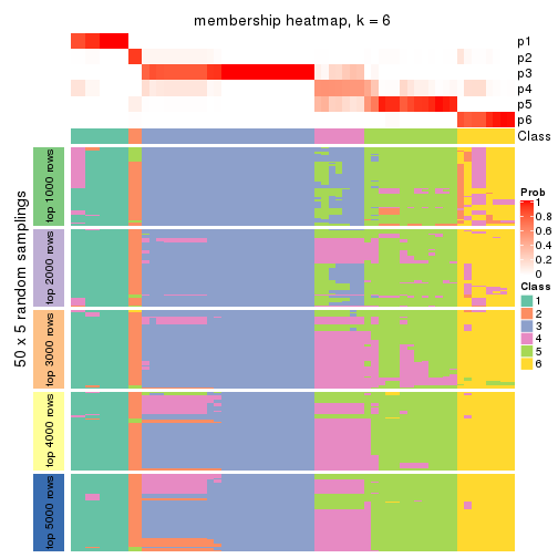
As soon as we have had the classes for columns, we can look for signatures which are significantly different between classes which can be candidate marks for certain classes. Following are the heatmaps for signatures.
Signature heatmaps where rows are scaled:
get_signatures(res, k = 2)

get_signatures(res, k = 3)
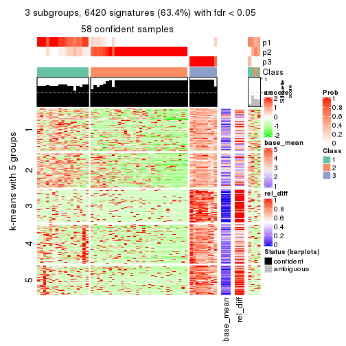
get_signatures(res, k = 4)
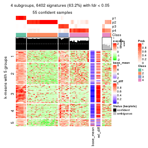
get_signatures(res, k = 5)
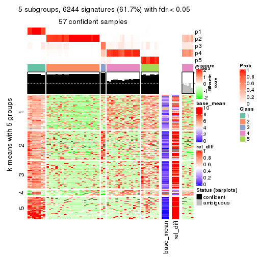
get_signatures(res, k = 6)
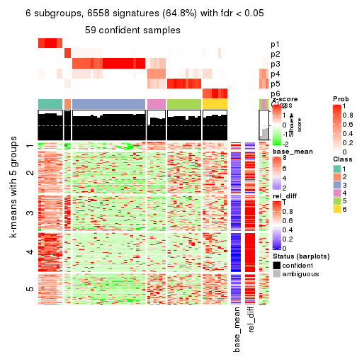
Signature heatmaps where rows are not scaled:
get_signatures(res, k = 2, scale_rows = FALSE)

get_signatures(res, k = 3, scale_rows = FALSE)
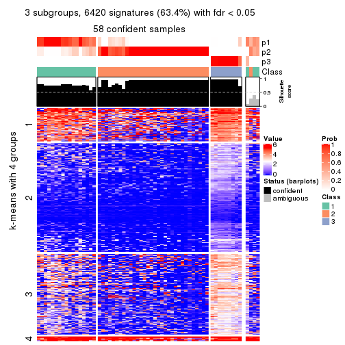
get_signatures(res, k = 4, scale_rows = FALSE)
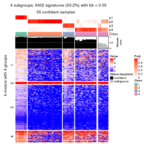
get_signatures(res, k = 5, scale_rows = FALSE)
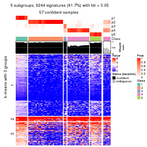
get_signatures(res, k = 6, scale_rows = FALSE)
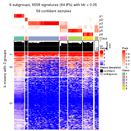
Compare the overlap of signatures from different k:
compare_signatures(res)
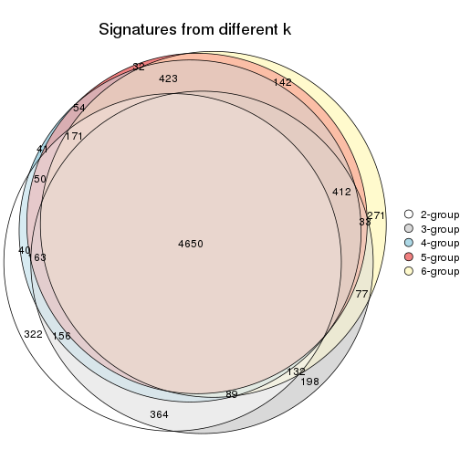
get_signature() returns a data frame invisibly. TO get the list of signatures, the function
call should be assigned to a variable explicitly. In following code, if plot argument is set
to FALSE, no heatmap is plotted while only the differential analysis is performed.
# code only for demonstration
tb = get_signature(res, k = ..., plot = FALSE)
An example of the output of tb is:
#> which_row fdr mean_1 mean_2 scaled_mean_1 scaled_mean_2 km
#> 1 38 0.042760348 8.373488 9.131774 -0.5533452 0.5164555 1
#> 2 40 0.018707592 7.106213 8.469186 -0.6173731 0.5762149 1
#> 3 55 0.019134737 10.221463 11.207825 -0.6159697 0.5749050 1
#> 4 59 0.006059896 5.921854 7.869574 -0.6899429 0.6439467 1
#> 5 60 0.018055526 8.928898 10.211722 -0.6204761 0.5791110 1
#> 6 98 0.009384629 15.714769 14.887706 0.6635654 -0.6193277 2
...
The columns in tb are:
which_row: row indices corresponding to the input matrix.fdr: FDR for the differential test. mean_x: The mean value in group x.scaled_mean_x: The mean value in group x after rows are scaled.km: Row groups if k-means clustering is applied to rows.UMAP plot which shows how samples are separated.
dimension_reduction(res, k = 2, method = "UMAP")

dimension_reduction(res, k = 3, method = "UMAP")
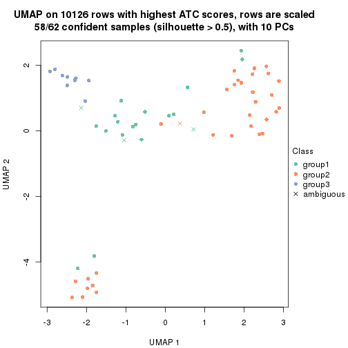
dimension_reduction(res, k = 4, method = "UMAP")
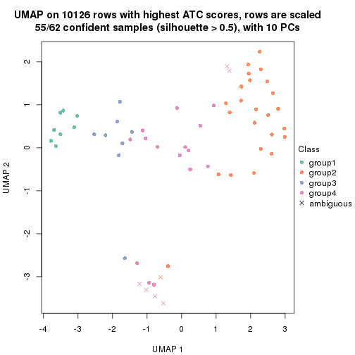
dimension_reduction(res, k = 5, method = "UMAP")
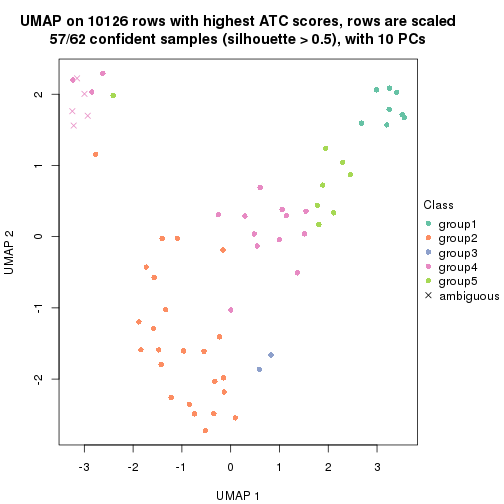
dimension_reduction(res, k = 6, method = "UMAP")
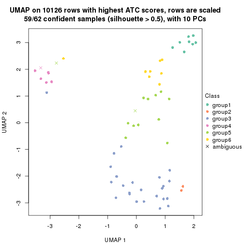
Following heatmap shows how subgroups are split when increasing k:
collect_classes(res)
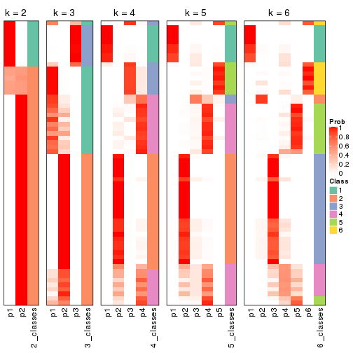
If matrix rows can be associated to genes, consider to use functional_enrichment(res,
...) to perform function enrichment for the signature genes. See this vignette for more detailed explanations.
The object with results only for a single top-value method and a single partition method can be extracted as:
res = res_list["ATC", "skmeans"]
# you can also extract it by
# res = res_list["ATC:skmeans"]
A summary of res and all the functions that can be applied to it:
res
#> A 'ConsensusPartition' object with k = 2, 3, 4, 5, 6.
#> On a matrix with 10126 rows and 62 columns.
#> Top rows (1000, 2000, 3000, 4000, 5000) are extracted by 'ATC' method.
#> Subgroups are detected by 'skmeans' method.
#> Performed in total 1250 partitions by row resampling.
#> Best k for subgroups seems to be 2.
#>
#> Following methods can be applied to this 'ConsensusPartition' object:
#> [1] "cola_report" "collect_classes" "collect_plots"
#> [4] "collect_stats" "colnames" "compare_signatures"
#> [7] "consensus_heatmap" "dimension_reduction" "functional_enrichment"
#> [10] "get_anno_col" "get_anno" "get_classes"
#> [13] "get_consensus" "get_matrix" "get_membership"
#> [16] "get_param" "get_signatures" "get_stats"
#> [19] "is_best_k" "is_stable_k" "membership_heatmap"
#> [22] "ncol" "nrow" "plot_ecdf"
#> [25] "rownames" "select_partition_number" "show"
#> [28] "suggest_best_k" "test_to_known_factors"
collect_plots() function collects all the plots made from res for all k (number of partitions)
into one single page to provide an easy and fast comparison between different k.
collect_plots(res)
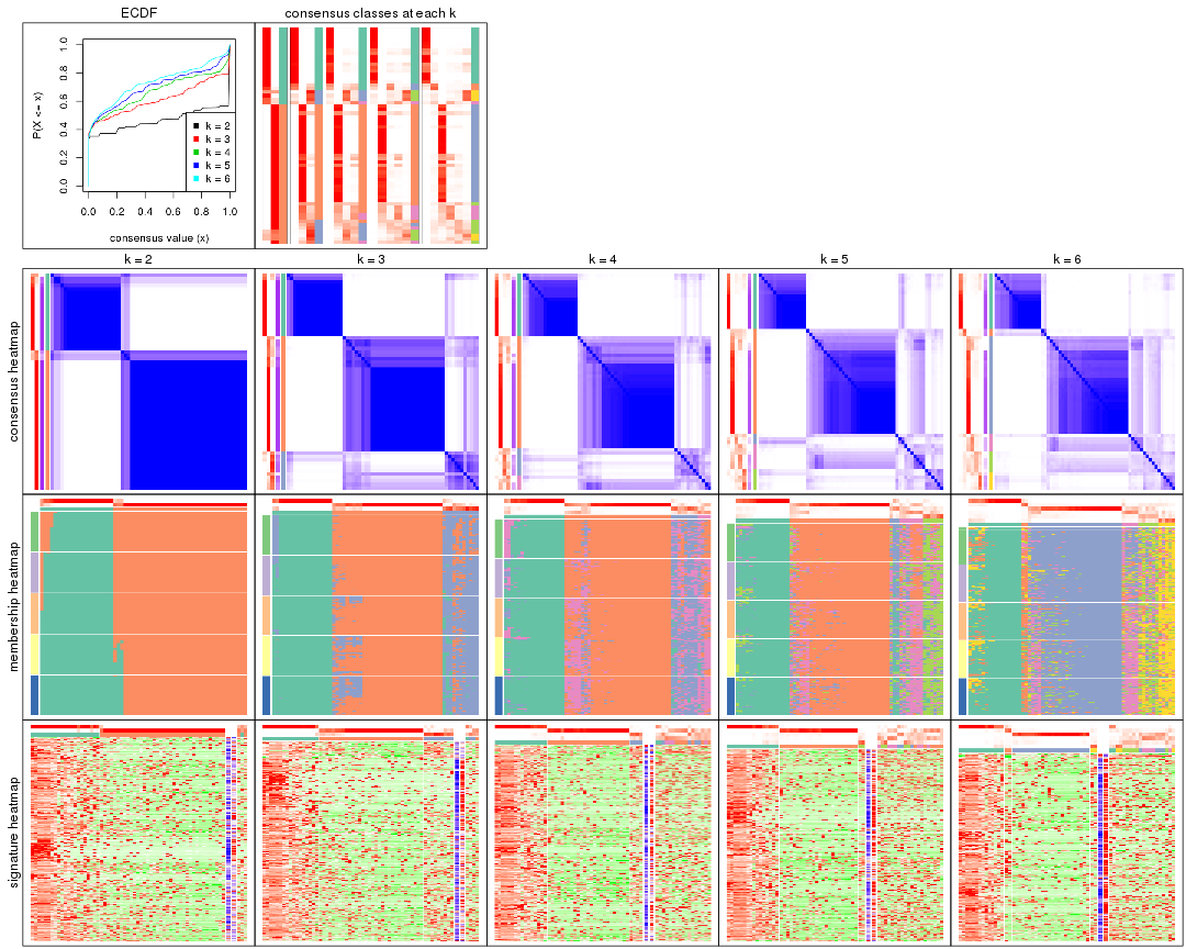
The plots are:
k and the heatmap of
predicted classes for each k.k.k.k.All the plots in panels can be made by individual functions and they are plotted later in this section.
select_partition_number() produces several plots showing different
statistics for choosing “optimized” k. There are following statistics:
k;k, the area increased is defined as \(A_k - A_{k-1}\).The detailed explanations of these statistics can be found in the cola vignette.
Generally speaking, lower PAC score, higher mean silhouette score or higher
concordance corresponds to better partition. Rand index and Jaccard index
measure how similar the current partition is compared to partition with k-1.
If they are too similar, we won't accept k is better than k-1.
select_partition_number(res)
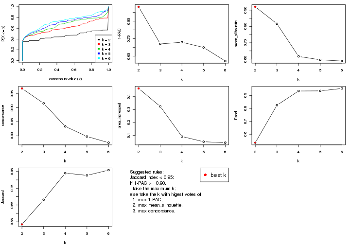
The numeric values for all these statistics can be obtained by get_stats().
get_stats(res)
#> k 1-PAC mean_silhouette concordance area_increased Rand Jaccard
#> 2 2 0.932 0.921 0.969 0.4629 0.535 0.535
#> 3 3 0.721 0.816 0.916 0.3236 0.825 0.681
#> 4 4 0.730 0.616 0.833 0.0917 0.935 0.840
#> 5 5 0.700 0.595 0.798 0.0515 0.936 0.827
#> 6 6 0.623 0.588 0.775 0.0441 0.955 0.858
suggest_best_k() suggests the best \(k\) based on these statistics. The rules are as follows:
suggest_best_k(res)
#> [1] 2
Following shows the table of the partitions (You need to click the show/hide
code output link to see it). The membership matrix (columns with name p*)
is inferred by
clue::cl_consensus()
function with the SE method. Basically the value in the membership matrix
represents the probability to belong to a certain group. The finall class
label for an item is determined with the group with highest probability it
belongs to.
In get_classes() function, the entropy is calculated from the membership
matrix and the silhouette score is calculated from the consensus matrix.
cbind(get_classes(res, k = 2), get_membership(res, k = 2))
#> class entropy silhouette p1 p2
#> SRR764776 1 0.0000 0.9510 1.000 0.000
#> SRR764777 1 0.0000 0.9510 1.000 0.000
#> SRR764778 1 0.0000 0.9510 1.000 0.000
#> SRR764779 1 0.0000 0.9510 1.000 0.000
#> SRR764780 1 0.0000 0.9510 1.000 0.000
#> SRR764781 1 0.0000 0.9510 1.000 0.000
#> SRR764782 1 0.9996 0.0452 0.512 0.488
#> SRR764783 1 0.0000 0.9510 1.000 0.000
#> SRR764784 2 0.9393 0.4237 0.356 0.644
#> SRR764785 2 0.0000 0.9734 0.000 1.000
#> SRR764786 2 0.0000 0.9734 0.000 1.000
#> SRR764787 2 0.0000 0.9734 0.000 1.000
#> SRR764788 1 0.0672 0.9457 0.992 0.008
#> SRR764789 2 0.0000 0.9734 0.000 1.000
#> SRR764790 2 0.0000 0.9734 0.000 1.000
#> SRR764791 2 0.0000 0.9734 0.000 1.000
#> SRR764792 2 0.0000 0.9734 0.000 1.000
#> SRR764793 2 0.8267 0.6283 0.260 0.740
#> SRR764794 2 0.0000 0.9734 0.000 1.000
#> SRR764795 1 0.7139 0.7542 0.804 0.196
#> SRR764796 2 0.9248 0.4629 0.340 0.660
#> SRR764797 1 0.0000 0.9510 1.000 0.000
#> SRR764798 1 0.0000 0.9510 1.000 0.000
#> SRR764799 1 0.0000 0.9510 1.000 0.000
#> SRR764800 1 0.0000 0.9510 1.000 0.000
#> SRR764801 1 0.4022 0.8859 0.920 0.080
#> SRR764802 1 0.0000 0.9510 1.000 0.000
#> SRR764803 1 0.0000 0.9510 1.000 0.000
#> SRR764804 2 0.0000 0.9734 0.000 1.000
#> SRR764805 2 0.0000 0.9734 0.000 1.000
#> SRR764806 2 0.0000 0.9734 0.000 1.000
#> SRR764807 2 0.0000 0.9734 0.000 1.000
#> SRR764808 2 0.0000 0.9734 0.000 1.000
#> SRR764809 2 0.0000 0.9734 0.000 1.000
#> SRR764810 2 0.0000 0.9734 0.000 1.000
#> SRR764811 2 0.0000 0.9734 0.000 1.000
#> SRR764812 2 0.0000 0.9734 0.000 1.000
#> SRR764813 2 0.0000 0.9734 0.000 1.000
#> SRR764814 1 0.0000 0.9510 1.000 0.000
#> SRR764815 2 0.0000 0.9734 0.000 1.000
#> SRR764816 1 0.0000 0.9510 1.000 0.000
#> SRR764817 1 0.0000 0.9510 1.000 0.000
#> SRR1066622 2 0.0000 0.9734 0.000 1.000
#> SRR1066623 2 0.0000 0.9734 0.000 1.000
#> SRR1066624 1 0.0000 0.9510 1.000 0.000
#> SRR1066625 1 0.7299 0.7430 0.796 0.204
#> SRR1066626 2 0.0000 0.9734 0.000 1.000
#> SRR1066627 2 0.0000 0.9734 0.000 1.000
#> SRR1066628 2 0.0000 0.9734 0.000 1.000
#> SRR1066629 2 0.0000 0.9734 0.000 1.000
#> SRR1066630 2 0.0000 0.9734 0.000 1.000
#> SRR1066631 2 0.0000 0.9734 0.000 1.000
#> SRR1066632 2 0.0000 0.9734 0.000 1.000
#> SRR1066633 2 0.0000 0.9734 0.000 1.000
#> SRR1066634 2 0.0000 0.9734 0.000 1.000
#> SRR1066635 2 0.0000 0.9734 0.000 1.000
#> SRR1066636 2 0.0000 0.9734 0.000 1.000
#> SRR1066637 2 0.0000 0.9734 0.000 1.000
#> SRR1066638 2 0.0000 0.9734 0.000 1.000
#> SRR1066639 2 0.0000 0.9734 0.000 1.000
#> SRR1066640 2 0.0000 0.9734 0.000 1.000
#> SRR1066641 2 0.0000 0.9734 0.000 1.000
cbind(get_classes(res, k = 3), get_membership(res, k = 3))
#> class entropy silhouette p1 p2 p3
#> SRR764776 1 0.0000 0.962 1.000 0.000 0.000
#> SRR764777 1 0.0000 0.962 1.000 0.000 0.000
#> SRR764778 1 0.0000 0.962 1.000 0.000 0.000
#> SRR764779 1 0.0000 0.962 1.000 0.000 0.000
#> SRR764780 1 0.0000 0.962 1.000 0.000 0.000
#> SRR764781 1 0.0000 0.962 1.000 0.000 0.000
#> SRR764782 3 0.0892 0.722 0.020 0.000 0.980
#> SRR764783 1 0.0000 0.962 1.000 0.000 0.000
#> SRR764784 3 0.1289 0.744 0.000 0.032 0.968
#> SRR764785 2 0.0000 0.916 0.000 1.000 0.000
#> SRR764786 2 0.0000 0.916 0.000 1.000 0.000
#> SRR764787 3 0.5650 0.573 0.000 0.312 0.688
#> SRR764788 3 0.4291 0.605 0.180 0.000 0.820
#> SRR764789 2 0.5529 0.570 0.000 0.704 0.296
#> SRR764790 2 0.0000 0.916 0.000 1.000 0.000
#> SRR764791 2 0.6244 0.105 0.000 0.560 0.440
#> SRR764792 3 0.5835 0.550 0.000 0.340 0.660
#> SRR764793 3 0.2749 0.755 0.012 0.064 0.924
#> SRR764794 3 0.6309 0.122 0.000 0.500 0.500
#> SRR764795 3 0.3267 0.675 0.116 0.000 0.884
#> SRR764796 3 0.3816 0.740 0.000 0.148 0.852
#> SRR764797 1 0.0000 0.962 1.000 0.000 0.000
#> SRR764798 1 0.5138 0.672 0.748 0.000 0.252
#> SRR764799 1 0.0000 0.962 1.000 0.000 0.000
#> SRR764800 1 0.0000 0.962 1.000 0.000 0.000
#> SRR764801 1 0.6275 0.485 0.644 0.008 0.348
#> SRR764802 1 0.0424 0.954 0.992 0.000 0.008
#> SRR764803 1 0.0000 0.962 1.000 0.000 0.000
#> SRR764804 2 0.0000 0.916 0.000 1.000 0.000
#> SRR764805 2 0.0000 0.916 0.000 1.000 0.000
#> SRR764806 2 0.0000 0.916 0.000 1.000 0.000
#> SRR764807 2 0.0000 0.916 0.000 1.000 0.000
#> SRR764808 2 0.0000 0.916 0.000 1.000 0.000
#> SRR764809 2 0.0000 0.916 0.000 1.000 0.000
#> SRR764810 2 0.0000 0.916 0.000 1.000 0.000
#> SRR764811 2 0.0000 0.916 0.000 1.000 0.000
#> SRR764812 2 0.0000 0.916 0.000 1.000 0.000
#> SRR764813 2 0.0000 0.916 0.000 1.000 0.000
#> SRR764814 1 0.0000 0.962 1.000 0.000 0.000
#> SRR764815 3 0.5315 0.700 0.012 0.216 0.772
#> SRR764816 1 0.0000 0.962 1.000 0.000 0.000
#> SRR764817 1 0.0000 0.962 1.000 0.000 0.000
#> SRR1066622 2 0.4796 0.714 0.000 0.780 0.220
#> SRR1066623 2 0.4974 0.692 0.000 0.764 0.236
#> SRR1066624 1 0.0000 0.962 1.000 0.000 0.000
#> SRR1066625 3 0.7163 0.369 0.332 0.040 0.628
#> SRR1066626 2 0.3038 0.838 0.000 0.896 0.104
#> SRR1066627 2 0.5678 0.550 0.000 0.684 0.316
#> SRR1066628 2 0.4235 0.768 0.000 0.824 0.176
#> SRR1066629 2 0.5760 0.522 0.000 0.672 0.328
#> SRR1066630 2 0.0000 0.916 0.000 1.000 0.000
#> SRR1066631 2 0.4002 0.785 0.000 0.840 0.160
#> SRR1066632 2 0.0000 0.916 0.000 1.000 0.000
#> SRR1066633 2 0.0000 0.916 0.000 1.000 0.000
#> SRR1066634 2 0.0000 0.916 0.000 1.000 0.000
#> SRR1066635 2 0.0000 0.916 0.000 1.000 0.000
#> SRR1066636 2 0.0000 0.916 0.000 1.000 0.000
#> SRR1066637 2 0.0000 0.916 0.000 1.000 0.000
#> SRR1066638 2 0.0000 0.916 0.000 1.000 0.000
#> SRR1066639 2 0.0000 0.916 0.000 1.000 0.000
#> SRR1066640 2 0.0000 0.916 0.000 1.000 0.000
#> SRR1066641 2 0.0000 0.916 0.000 1.000 0.000
cbind(get_classes(res, k = 4), get_membership(res, k = 4))
#> class entropy silhouette p1 p2 p3 p4
#> SRR764776 1 0.0000 0.9180 1.000 0.000 0.000 0.000
#> SRR764777 1 0.0000 0.9180 1.000 0.000 0.000 0.000
#> SRR764778 1 0.0000 0.9180 1.000 0.000 0.000 0.000
#> SRR764779 1 0.0000 0.9180 1.000 0.000 0.000 0.000
#> SRR764780 1 0.0000 0.9180 1.000 0.000 0.000 0.000
#> SRR764781 1 0.0000 0.9180 1.000 0.000 0.000 0.000
#> SRR764782 3 0.3760 0.5775 0.028 0.000 0.836 0.136
#> SRR764783 1 0.1975 0.8907 0.936 0.000 0.048 0.016
#> SRR764784 3 0.4671 0.5635 0.000 0.028 0.752 0.220
#> SRR764785 2 0.0672 0.8275 0.000 0.984 0.008 0.008
#> SRR764786 2 0.0000 0.8334 0.000 1.000 0.000 0.000
#> SRR764787 4 0.7796 -0.0338 0.000 0.248 0.360 0.392
#> SRR764788 3 0.5742 0.4751 0.168 0.000 0.712 0.120
#> SRR764789 2 0.6916 0.0644 0.000 0.588 0.176 0.236
#> SRR764790 2 0.0000 0.8334 0.000 1.000 0.000 0.000
#> SRR764791 2 0.7805 -0.4082 0.000 0.420 0.280 0.300
#> SRR764792 3 0.7782 -0.0559 0.000 0.264 0.424 0.312
#> SRR764793 3 0.5511 0.5183 0.000 0.028 0.620 0.352
#> SRR764794 2 0.7884 -0.4184 0.000 0.384 0.308 0.308
#> SRR764795 3 0.4919 0.5444 0.076 0.000 0.772 0.152
#> SRR764796 3 0.6639 0.4124 0.004 0.092 0.584 0.320
#> SRR764797 1 0.2830 0.8710 0.900 0.000 0.060 0.040
#> SRR764798 1 0.7048 0.3843 0.556 0.000 0.160 0.284
#> SRR764799 1 0.0000 0.9180 1.000 0.000 0.000 0.000
#> SRR764800 1 0.0000 0.9180 1.000 0.000 0.000 0.000
#> SRR764801 1 0.7850 0.0740 0.432 0.004 0.228 0.336
#> SRR764802 1 0.3099 0.8477 0.876 0.000 0.104 0.020
#> SRR764803 1 0.2111 0.8913 0.932 0.000 0.044 0.024
#> SRR764804 2 0.0000 0.8334 0.000 1.000 0.000 0.000
#> SRR764805 2 0.0000 0.8334 0.000 1.000 0.000 0.000
#> SRR764806 2 0.0927 0.8197 0.000 0.976 0.008 0.016
#> SRR764807 2 0.0000 0.8334 0.000 1.000 0.000 0.000
#> SRR764808 2 0.0000 0.8334 0.000 1.000 0.000 0.000
#> SRR764809 2 0.0000 0.8334 0.000 1.000 0.000 0.000
#> SRR764810 2 0.0000 0.8334 0.000 1.000 0.000 0.000
#> SRR764811 2 0.0000 0.8334 0.000 1.000 0.000 0.000
#> SRR764812 2 0.0000 0.8334 0.000 1.000 0.000 0.000
#> SRR764813 2 0.0000 0.8334 0.000 1.000 0.000 0.000
#> SRR764814 1 0.2089 0.8911 0.932 0.000 0.048 0.020
#> SRR764815 3 0.7583 0.2126 0.012 0.136 0.436 0.416
#> SRR764816 1 0.0000 0.9180 1.000 0.000 0.000 0.000
#> SRR764817 1 0.0000 0.9180 1.000 0.000 0.000 0.000
#> SRR1066622 2 0.5861 -0.2995 0.000 0.492 0.032 0.476
#> SRR1066623 2 0.6252 -0.2341 0.000 0.512 0.056 0.432
#> SRR1066624 1 0.0376 0.9157 0.992 0.000 0.004 0.004
#> SRR1066625 4 0.6833 -0.3487 0.128 0.012 0.232 0.628
#> SRR1066626 2 0.4502 0.5119 0.000 0.748 0.016 0.236
#> SRR1066627 4 0.6546 0.4327 0.000 0.396 0.080 0.524
#> SRR1066628 2 0.5510 0.1039 0.000 0.600 0.024 0.376
#> SRR1066629 4 0.6554 0.4317 0.000 0.376 0.084 0.540
#> SRR1066630 2 0.0000 0.8334 0.000 1.000 0.000 0.000
#> SRR1066631 2 0.5407 0.3307 0.000 0.668 0.036 0.296
#> SRR1066632 2 0.0804 0.8259 0.000 0.980 0.008 0.012
#> SRR1066633 2 0.1488 0.8084 0.000 0.956 0.012 0.032
#> SRR1066634 2 0.1211 0.8101 0.000 0.960 0.000 0.040
#> SRR1066635 2 0.0000 0.8334 0.000 1.000 0.000 0.000
#> SRR1066636 2 0.0000 0.8334 0.000 1.000 0.000 0.000
#> SRR1066637 2 0.1488 0.8100 0.000 0.956 0.012 0.032
#> SRR1066638 2 0.1004 0.8210 0.000 0.972 0.004 0.024
#> SRR1066639 2 0.0188 0.8317 0.000 0.996 0.000 0.004
#> SRR1066640 2 0.0188 0.8318 0.000 0.996 0.000 0.004
#> SRR1066641 2 0.0000 0.8334 0.000 1.000 0.000 0.000
cbind(get_classes(res, k = 5), get_membership(res, k = 5))
#> class entropy silhouette p1 p2 p3 p4 p5
#> SRR764776 1 0.0000 0.911 1.000 0.000 0.000 0.000 0.000
#> SRR764777 1 0.0000 0.911 1.000 0.000 0.000 0.000 0.000
#> SRR764778 1 0.0000 0.911 1.000 0.000 0.000 0.000 0.000
#> SRR764779 1 0.0000 0.911 1.000 0.000 0.000 0.000 0.000
#> SRR764780 1 0.0162 0.910 0.996 0.000 0.000 0.004 0.000
#> SRR764781 1 0.0162 0.910 0.996 0.000 0.000 0.004 0.000
#> SRR764782 5 0.3586 0.559 0.000 0.000 0.096 0.076 0.828
#> SRR764783 1 0.3963 0.782 0.820 0.000 0.036 0.032 0.112
#> SRR764784 5 0.5229 0.551 0.000 0.020 0.080 0.192 0.708
#> SRR764785 2 0.2283 0.790 0.000 0.916 0.040 0.036 0.008
#> SRR764786 2 0.0162 0.833 0.000 0.996 0.000 0.004 0.000
#> SRR764787 4 0.8571 0.126 0.000 0.216 0.268 0.288 0.228
#> SRR764788 5 0.6261 0.393 0.124 0.000 0.148 0.072 0.656
#> SRR764789 2 0.7415 -0.107 0.000 0.520 0.160 0.224 0.096
#> SRR764790 2 0.0000 0.833 0.000 1.000 0.000 0.000 0.000
#> SRR764791 2 0.8214 -0.402 0.000 0.392 0.228 0.240 0.140
#> SRR764792 3 0.8296 -0.342 0.000 0.164 0.348 0.180 0.308
#> SRR764793 5 0.7371 0.397 0.004 0.036 0.232 0.260 0.468
#> SRR764794 2 0.8524 -0.510 0.000 0.284 0.268 0.268 0.180
#> SRR764795 5 0.5209 0.489 0.068 0.000 0.100 0.084 0.748
#> SRR764796 5 0.7505 0.408 0.008 0.064 0.132 0.344 0.452
#> SRR764797 1 0.5422 0.652 0.728 0.000 0.088 0.060 0.124
#> SRR764798 3 0.5770 0.262 0.392 0.000 0.540 0.028 0.040
#> SRR764799 1 0.0000 0.911 1.000 0.000 0.000 0.000 0.000
#> SRR764800 1 0.0000 0.911 1.000 0.000 0.000 0.000 0.000
#> SRR764801 3 0.6207 0.215 0.224 0.000 0.624 0.036 0.116
#> SRR764802 1 0.5540 0.595 0.700 0.000 0.092 0.036 0.172
#> SRR764803 1 0.3191 0.838 0.872 0.000 0.040 0.024 0.064
#> SRR764804 2 0.0000 0.833 0.000 1.000 0.000 0.000 0.000
#> SRR764805 2 0.0000 0.833 0.000 1.000 0.000 0.000 0.000
#> SRR764806 2 0.2110 0.793 0.000 0.912 0.072 0.016 0.000
#> SRR764807 2 0.0000 0.833 0.000 1.000 0.000 0.000 0.000
#> SRR764808 2 0.0000 0.833 0.000 1.000 0.000 0.000 0.000
#> SRR764809 2 0.0000 0.833 0.000 1.000 0.000 0.000 0.000
#> SRR764810 2 0.0000 0.833 0.000 1.000 0.000 0.000 0.000
#> SRR764811 2 0.0000 0.833 0.000 1.000 0.000 0.000 0.000
#> SRR764812 2 0.0000 0.833 0.000 1.000 0.000 0.000 0.000
#> SRR764813 2 0.0000 0.833 0.000 1.000 0.000 0.000 0.000
#> SRR764814 1 0.4435 0.761 0.800 0.000 0.080 0.044 0.076
#> SRR764815 4 0.8032 -0.236 0.000 0.088 0.308 0.348 0.256
#> SRR764816 1 0.0000 0.911 1.000 0.000 0.000 0.000 0.000
#> SRR764817 1 0.0000 0.911 1.000 0.000 0.000 0.000 0.000
#> SRR1066622 4 0.5841 0.462 0.000 0.396 0.044 0.532 0.028
#> SRR1066623 4 0.6078 0.394 0.000 0.424 0.048 0.492 0.036
#> SRR1066624 1 0.1893 0.869 0.928 0.000 0.048 0.024 0.000
#> SRR1066625 4 0.7514 -0.294 0.068 0.012 0.264 0.512 0.144
#> SRR1066626 2 0.5400 0.257 0.000 0.640 0.048 0.292 0.020
#> SRR1066627 4 0.5486 0.529 0.000 0.304 0.040 0.628 0.028
#> SRR1066628 2 0.5545 -0.225 0.000 0.516 0.032 0.432 0.020
#> SRR1066629 4 0.5954 0.492 0.000 0.264 0.060 0.628 0.048
#> SRR1066630 2 0.0000 0.833 0.000 1.000 0.000 0.000 0.000
#> SRR1066631 2 0.5483 0.193 0.000 0.616 0.052 0.316 0.016
#> SRR1066632 2 0.1996 0.806 0.000 0.928 0.036 0.032 0.004
#> SRR1066633 2 0.3114 0.752 0.000 0.872 0.076 0.036 0.016
#> SRR1066634 2 0.1965 0.802 0.000 0.924 0.052 0.024 0.000
#> SRR1066635 2 0.0566 0.831 0.000 0.984 0.004 0.012 0.000
#> SRR1066636 2 0.1492 0.818 0.000 0.948 0.040 0.004 0.008
#> SRR1066637 2 0.1800 0.809 0.000 0.932 0.048 0.020 0.000
#> SRR1066638 2 0.1202 0.821 0.000 0.960 0.032 0.004 0.004
#> SRR1066639 2 0.0671 0.830 0.000 0.980 0.016 0.004 0.000
#> SRR1066640 2 0.1739 0.814 0.000 0.940 0.032 0.024 0.004
#> SRR1066641 2 0.0000 0.833 0.000 1.000 0.000 0.000 0.000
cbind(get_classes(res, k = 6), get_membership(res, k = 6))
#> class entropy silhouette p1 p2 p3 p4 p5 p6
#> SRR764776 1 0.0000 0.8655 1.000 0.000 0.000 0.000 0.000 0.000
#> SRR764777 1 0.0000 0.8655 1.000 0.000 0.000 0.000 0.000 0.000
#> SRR764778 1 0.0000 0.8655 1.000 0.000 0.000 0.000 0.000 0.000
#> SRR764779 1 0.0000 0.8655 1.000 0.000 0.000 0.000 0.000 0.000
#> SRR764780 1 0.0405 0.8618 0.988 0.000 0.000 0.000 0.004 0.008
#> SRR764781 1 0.0767 0.8575 0.976 0.000 0.000 0.004 0.008 0.012
#> SRR764782 6 0.4180 0.5515 0.000 0.056 0.000 0.056 0.104 0.784
#> SRR764783 1 0.5186 0.6494 0.708 0.064 0.000 0.024 0.036 0.168
#> SRR764784 6 0.5907 0.4555 0.000 0.048 0.020 0.112 0.176 0.644
#> SRR764785 3 0.2906 0.7856 0.000 0.040 0.876 0.028 0.052 0.004
#> SRR764786 3 0.0717 0.8397 0.000 0.008 0.976 0.000 0.016 0.000
#> SRR764787 5 0.8413 0.2604 0.000 0.140 0.164 0.156 0.396 0.144
#> SRR764788 6 0.4876 0.4821 0.044 0.136 0.000 0.016 0.064 0.740
#> SRR764789 3 0.8070 -0.3689 0.000 0.072 0.412 0.228 0.168 0.120
#> SRR764790 3 0.0291 0.8417 0.000 0.004 0.992 0.000 0.004 0.000
#> SRR764791 5 0.8193 0.0922 0.000 0.084 0.308 0.156 0.344 0.108
#> SRR764792 5 0.8425 0.2876 0.000 0.124 0.188 0.128 0.384 0.176
#> SRR764793 5 0.7233 -0.2087 0.000 0.116 0.028 0.092 0.440 0.324
#> SRR764794 5 0.8191 0.2343 0.000 0.112 0.244 0.136 0.400 0.108
#> SRR764795 6 0.4682 0.5211 0.020 0.108 0.000 0.060 0.048 0.764
#> SRR764796 6 0.8012 0.2192 0.004 0.112 0.048 0.288 0.164 0.384
#> SRR764797 1 0.6319 0.4984 0.624 0.104 0.000 0.032 0.076 0.164
#> SRR764798 2 0.5353 0.6543 0.216 0.672 0.000 0.032 0.024 0.056
#> SRR764799 1 0.0000 0.8655 1.000 0.000 0.000 0.000 0.000 0.000
#> SRR764800 1 0.0000 0.8655 1.000 0.000 0.000 0.000 0.000 0.000
#> SRR764801 2 0.4461 0.6238 0.104 0.784 0.004 0.024 0.028 0.056
#> SRR764802 1 0.6159 0.4682 0.608 0.076 0.000 0.044 0.040 0.232
#> SRR764803 1 0.5595 0.6132 0.688 0.068 0.000 0.028 0.064 0.152
#> SRR764804 3 0.0000 0.8416 0.000 0.000 1.000 0.000 0.000 0.000
#> SRR764805 3 0.0363 0.8417 0.000 0.000 0.988 0.000 0.012 0.000
#> SRR764806 3 0.3811 0.7390 0.000 0.056 0.820 0.052 0.068 0.004
#> SRR764807 3 0.0000 0.8416 0.000 0.000 1.000 0.000 0.000 0.000
#> SRR764808 3 0.0000 0.8416 0.000 0.000 1.000 0.000 0.000 0.000
#> SRR764809 3 0.0000 0.8416 0.000 0.000 1.000 0.000 0.000 0.000
#> SRR764810 3 0.0000 0.8416 0.000 0.000 1.000 0.000 0.000 0.000
#> SRR764811 3 0.0146 0.8419 0.000 0.000 0.996 0.000 0.004 0.000
#> SRR764812 3 0.0000 0.8416 0.000 0.000 1.000 0.000 0.000 0.000
#> SRR764813 3 0.0146 0.8419 0.000 0.000 0.996 0.000 0.004 0.000
#> SRR764814 1 0.5317 0.6236 0.704 0.108 0.000 0.020 0.036 0.132
#> SRR764815 5 0.8393 0.0641 0.004 0.148 0.068 0.240 0.364 0.176
#> SRR764816 1 0.0000 0.8655 1.000 0.000 0.000 0.000 0.000 0.000
#> SRR764817 1 0.0000 0.8655 1.000 0.000 0.000 0.000 0.000 0.000
#> SRR1066622 4 0.5536 0.4057 0.000 0.016 0.340 0.572 0.036 0.036
#> SRR1066623 4 0.6345 0.4129 0.000 0.044 0.320 0.528 0.084 0.024
#> SRR1066624 1 0.2518 0.8032 0.892 0.060 0.000 0.008 0.036 0.004
#> SRR1066625 4 0.7946 -0.3372 0.080 0.276 0.000 0.404 0.152 0.088
#> SRR1066626 3 0.5817 -0.0210 0.000 0.044 0.544 0.328 0.084 0.000
#> SRR1066627 4 0.5717 0.3895 0.000 0.020 0.220 0.644 0.064 0.052
#> SRR1066628 3 0.5901 -0.3327 0.000 0.036 0.476 0.420 0.052 0.016
#> SRR1066629 4 0.6146 0.4168 0.000 0.040 0.244 0.600 0.080 0.036
#> SRR1066630 3 0.0405 0.8413 0.000 0.004 0.988 0.000 0.008 0.000
#> SRR1066631 3 0.6089 -0.1847 0.000 0.024 0.504 0.356 0.104 0.012
#> SRR1066632 3 0.3491 0.7591 0.000 0.056 0.840 0.036 0.064 0.004
#> SRR1066633 3 0.4021 0.7158 0.000 0.044 0.808 0.036 0.096 0.016
#> SRR1066634 3 0.3298 0.7682 0.000 0.020 0.848 0.056 0.072 0.004
#> SRR1066635 3 0.1078 0.8370 0.000 0.012 0.964 0.008 0.016 0.000
#> SRR1066636 3 0.1647 0.8303 0.000 0.016 0.940 0.008 0.032 0.004
#> SRR1066637 3 0.3582 0.7544 0.000 0.040 0.836 0.040 0.076 0.008
#> SRR1066638 3 0.3103 0.7729 0.000 0.040 0.860 0.060 0.040 0.000
#> SRR1066639 3 0.1364 0.8342 0.000 0.012 0.952 0.016 0.020 0.000
#> SRR1066640 3 0.2415 0.8089 0.000 0.024 0.900 0.036 0.040 0.000
#> SRR1066641 3 0.0000 0.8416 0.000 0.000 1.000 0.000 0.000 0.000
Heatmaps for the consensus matrix. It visualizes the probability of two samples to be in a same group.
consensus_heatmap(res, k = 2)
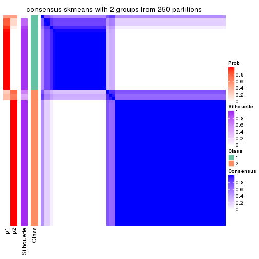
consensus_heatmap(res, k = 3)
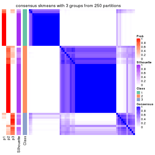
consensus_heatmap(res, k = 4)
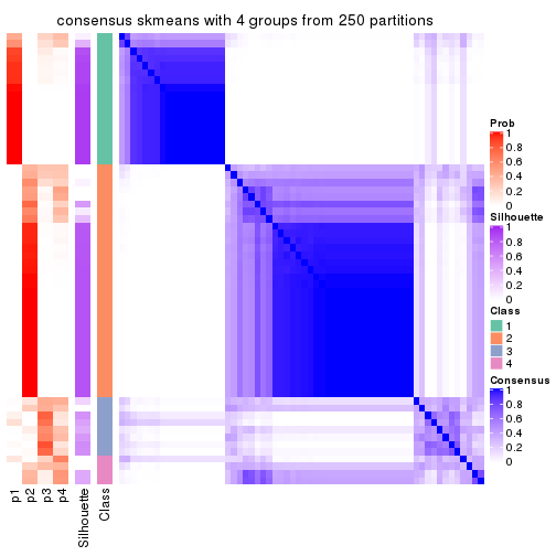
consensus_heatmap(res, k = 5)
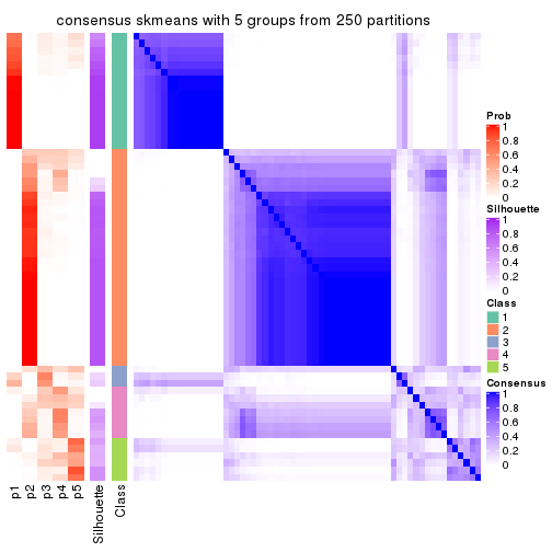
consensus_heatmap(res, k = 6)
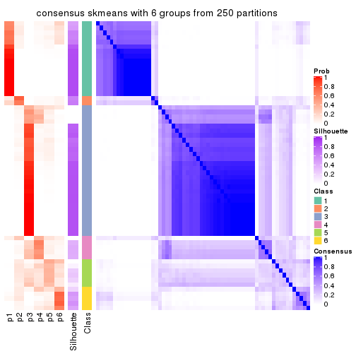
Heatmaps for the membership of samples in all partitions to see how consistent they are:
membership_heatmap(res, k = 2)
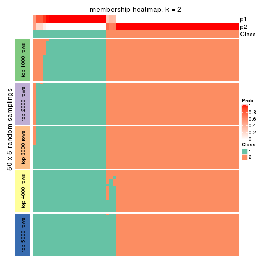
membership_heatmap(res, k = 3)
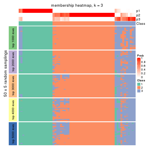
membership_heatmap(res, k = 4)
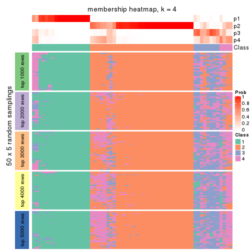
membership_heatmap(res, k = 5)
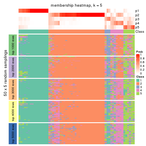
membership_heatmap(res, k = 6)
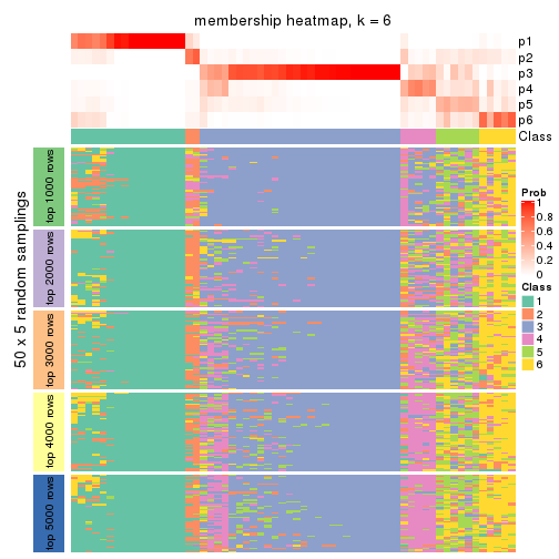
As soon as we have had the classes for columns, we can look for signatures which are significantly different between classes which can be candidate marks for certain classes. Following are the heatmaps for signatures.
Signature heatmaps where rows are scaled:
get_signatures(res, k = 2)
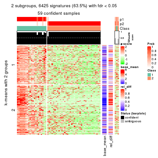
get_signatures(res, k = 3)
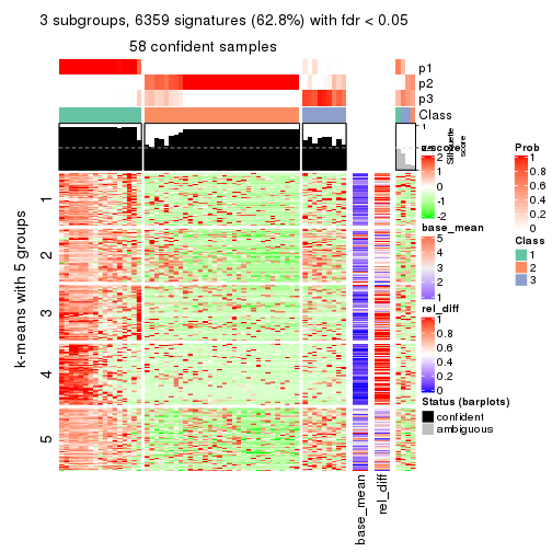
get_signatures(res, k = 4)
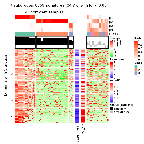
get_signatures(res, k = 5)
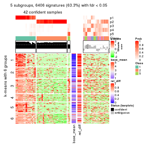
get_signatures(res, k = 6)
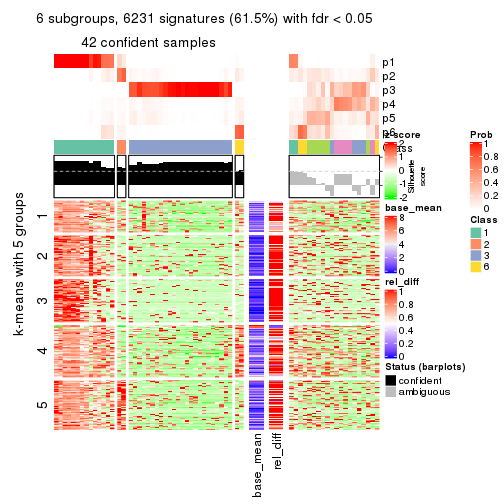
Signature heatmaps where rows are not scaled:
get_signatures(res, k = 2, scale_rows = FALSE)
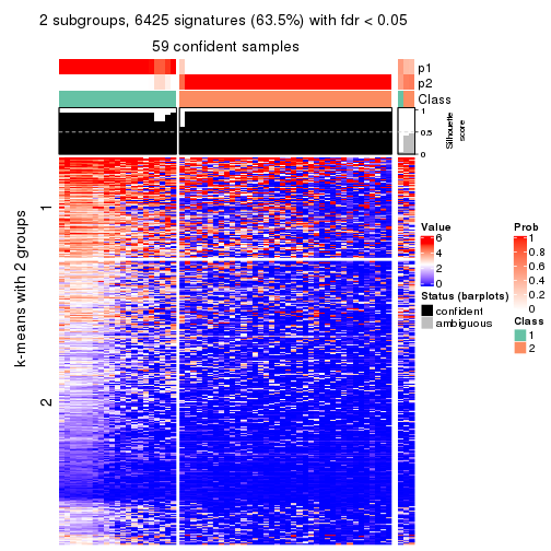
get_signatures(res, k = 3, scale_rows = FALSE)
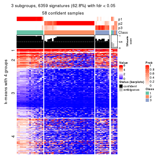
get_signatures(res, k = 4, scale_rows = FALSE)
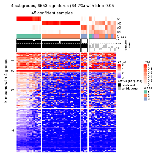
get_signatures(res, k = 5, scale_rows = FALSE)
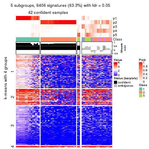
get_signatures(res, k = 6, scale_rows = FALSE)
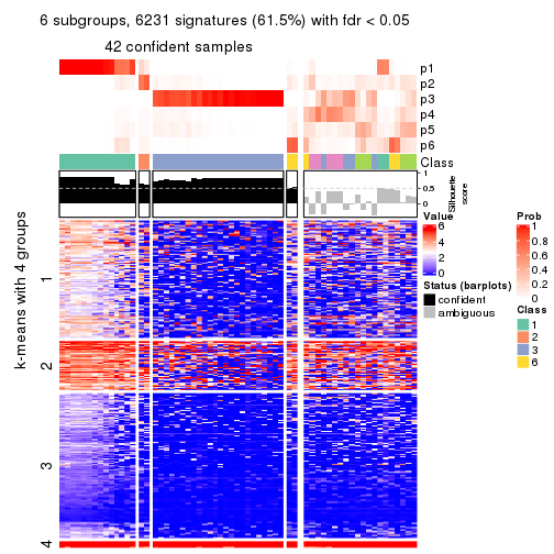
Compare the overlap of signatures from different k:
compare_signatures(res)
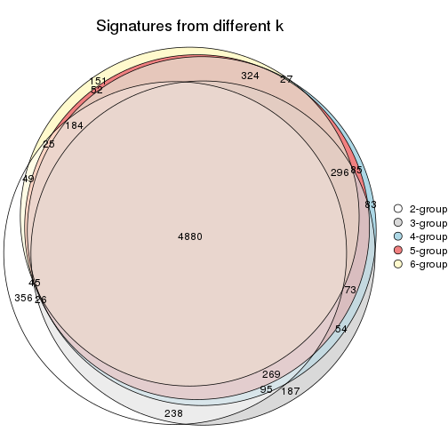
get_signature() returns a data frame invisibly. TO get the list of signatures, the function
call should be assigned to a variable explicitly. In following code, if plot argument is set
to FALSE, no heatmap is plotted while only the differential analysis is performed.
# code only for demonstration
tb = get_signature(res, k = ..., plot = FALSE)
An example of the output of tb is:
#> which_row fdr mean_1 mean_2 scaled_mean_1 scaled_mean_2 km
#> 1 38 0.042760348 8.373488 9.131774 -0.5533452 0.5164555 1
#> 2 40 0.018707592 7.106213 8.469186 -0.6173731 0.5762149 1
#> 3 55 0.019134737 10.221463 11.207825 -0.6159697 0.5749050 1
#> 4 59 0.006059896 5.921854 7.869574 -0.6899429 0.6439467 1
#> 5 60 0.018055526 8.928898 10.211722 -0.6204761 0.5791110 1
#> 6 98 0.009384629 15.714769 14.887706 0.6635654 -0.6193277 2
...
The columns in tb are:
which_row: row indices corresponding to the input matrix.fdr: FDR for the differential test. mean_x: The mean value in group x.scaled_mean_x: The mean value in group x after rows are scaled.km: Row groups if k-means clustering is applied to rows.UMAP plot which shows how samples are separated.
dimension_reduction(res, k = 2, method = "UMAP")
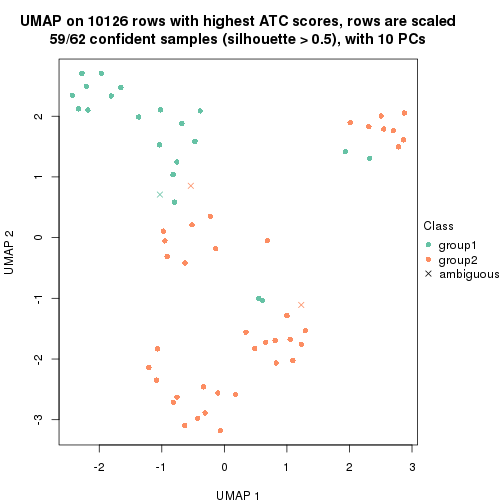
dimension_reduction(res, k = 3, method = "UMAP")
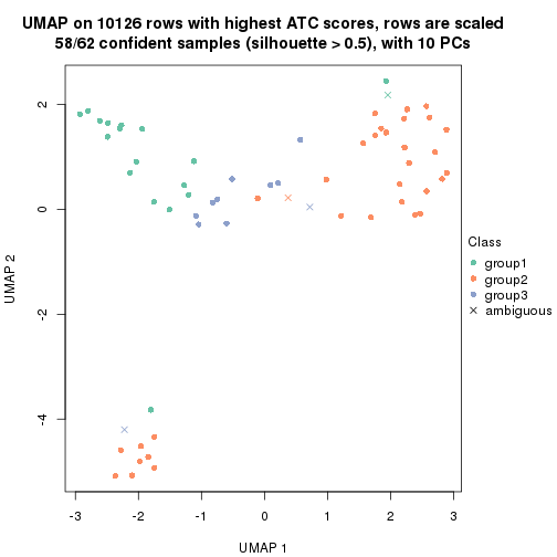
dimension_reduction(res, k = 4, method = "UMAP")
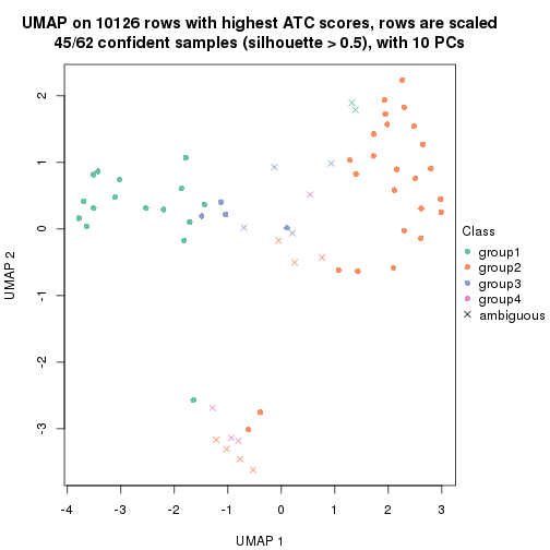
dimension_reduction(res, k = 5, method = "UMAP")
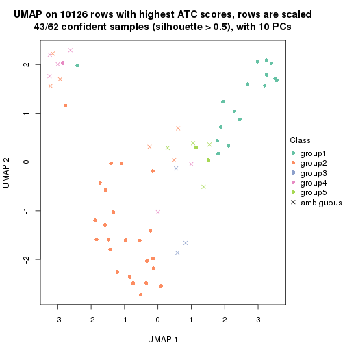
dimension_reduction(res, k = 6, method = "UMAP")
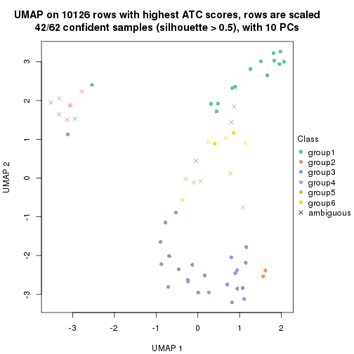
Following heatmap shows how subgroups are split when increasing k:
collect_classes(res)
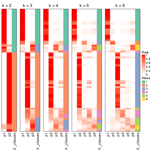
If matrix rows can be associated to genes, consider to use functional_enrichment(res,
...) to perform function enrichment for the signature genes. See this vignette for more detailed explanations.
The object with results only for a single top-value method and a single partition method can be extracted as:
res = res_list["ATC", "pam"]
# you can also extract it by
# res = res_list["ATC:pam"]
A summary of res and all the functions that can be applied to it:
res
#> A 'ConsensusPartition' object with k = 2, 3, 4, 5, 6.
#> On a matrix with 10126 rows and 62 columns.
#> Top rows (1000, 2000, 3000, 4000, 5000) are extracted by 'ATC' method.
#> Subgroups are detected by 'pam' method.
#> Performed in total 1250 partitions by row resampling.
#> Best k for subgroups seems to be 2.
#>
#> Following methods can be applied to this 'ConsensusPartition' object:
#> [1] "cola_report" "collect_classes" "collect_plots"
#> [4] "collect_stats" "colnames" "compare_signatures"
#> [7] "consensus_heatmap" "dimension_reduction" "functional_enrichment"
#> [10] "get_anno_col" "get_anno" "get_classes"
#> [13] "get_consensus" "get_matrix" "get_membership"
#> [16] "get_param" "get_signatures" "get_stats"
#> [19] "is_best_k" "is_stable_k" "membership_heatmap"
#> [22] "ncol" "nrow" "plot_ecdf"
#> [25] "rownames" "select_partition_number" "show"
#> [28] "suggest_best_k" "test_to_known_factors"
collect_plots() function collects all the plots made from res for all k (number of partitions)
into one single page to provide an easy and fast comparison between different k.
collect_plots(res)
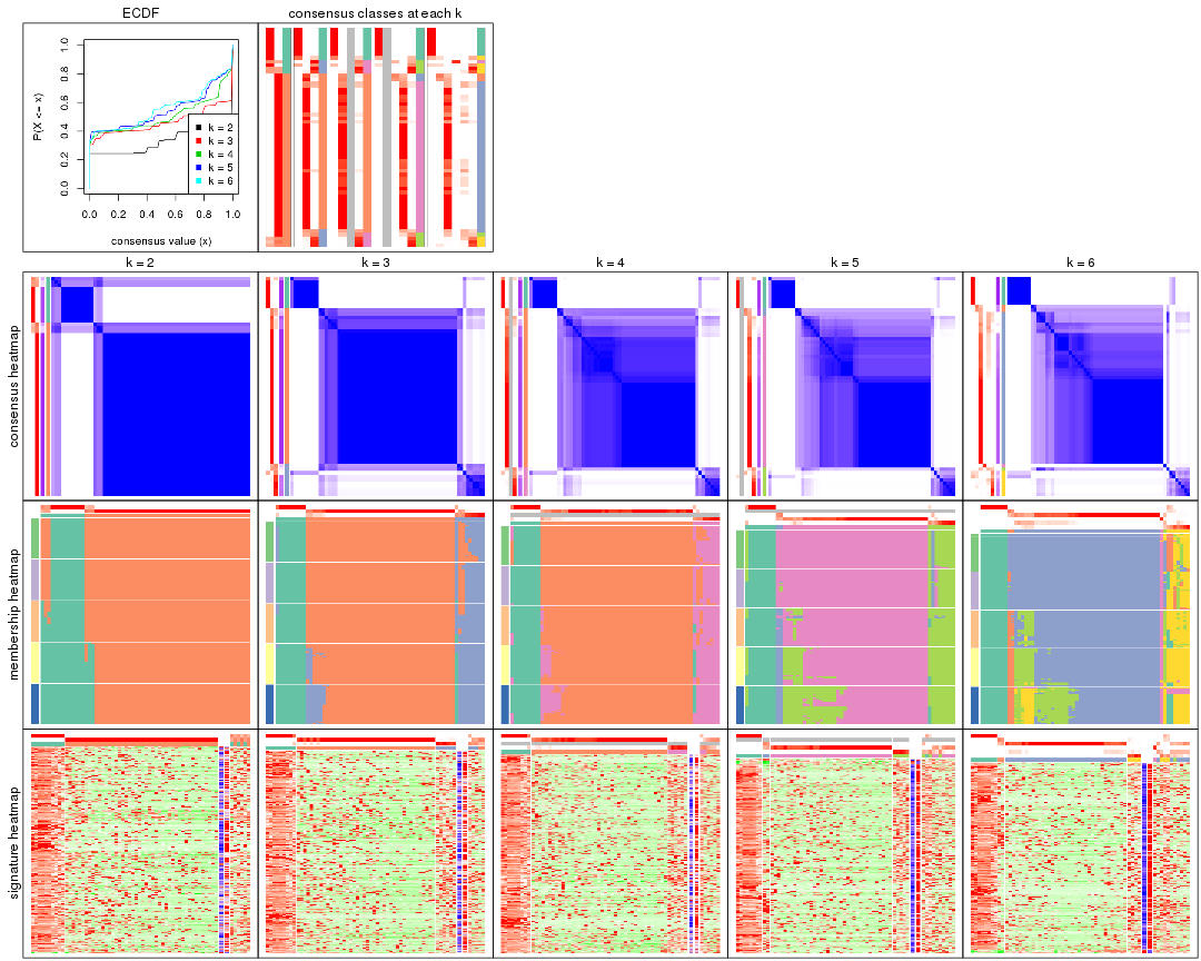
The plots are:
k and the heatmap of
predicted classes for each k.k.k.k.All the plots in panels can be made by individual functions and they are plotted later in this section.
select_partition_number() produces several plots showing different
statistics for choosing “optimized” k. There are following statistics:
k;k, the area increased is defined as \(A_k - A_{k-1}\).The detailed explanations of these statistics can be found in the cola vignette.
Generally speaking, lower PAC score, higher mean silhouette score or higher
concordance corresponds to better partition. Rand index and Jaccard index
measure how similar the current partition is compared to partition with k-1.
If they are too similar, we won't accept k is better than k-1.
select_partition_number(res)
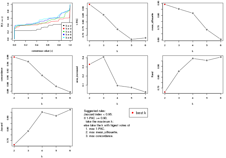
The numeric values for all these statistics can be obtained by get_stats().
get_stats(res)
#> k 1-PAC mean_silhouette concordance area_increased Rand Jaccard
#> 2 2 0.932 0.890 0.960 0.3288 0.663 0.663
#> 3 3 0.854 0.853 0.947 0.4084 0.854 0.783
#> 4 4 0.745 0.818 0.906 0.0948 0.973 0.951
#> 5 5 0.669 0.684 0.874 0.0738 0.955 0.918
#> 6 6 0.680 0.605 0.858 0.0241 0.986 0.972
suggest_best_k() suggests the best \(k\) based on these statistics. The rules are as follows:
suggest_best_k(res)
#> [1] 2
Following shows the table of the partitions (You need to click the show/hide
code output link to see it). The membership matrix (columns with name p*)
is inferred by
clue::cl_consensus()
function with the SE method. Basically the value in the membership matrix
represents the probability to belong to a certain group. The finall class
label for an item is determined with the group with highest probability it
belongs to.
In get_classes() function, the entropy is calculated from the membership
matrix and the silhouette score is calculated from the consensus matrix.
cbind(get_classes(res, k = 2), get_membership(res, k = 2))
#> class entropy silhouette p1 p2
#> SRR764776 1 0.000 0.879 1.000 0.000
#> SRR764777 1 0.000 0.879 1.000 0.000
#> SRR764778 1 0.000 0.879 1.000 0.000
#> SRR764779 1 0.000 0.879 1.000 0.000
#> SRR764780 1 0.000 0.879 1.000 0.000
#> SRR764781 1 0.000 0.879 1.000 0.000
#> SRR764782 2 0.000 0.973 0.000 1.000
#> SRR764783 1 0.999 0.168 0.520 0.480
#> SRR764784 2 0.000 0.973 0.000 1.000
#> SRR764785 2 0.000 0.973 0.000 1.000
#> SRR764786 2 0.000 0.973 0.000 1.000
#> SRR764787 2 0.000 0.973 0.000 1.000
#> SRR764788 2 0.000 0.973 0.000 1.000
#> SRR764789 2 0.000 0.973 0.000 1.000
#> SRR764790 2 0.000 0.973 0.000 1.000
#> SRR764791 2 0.000 0.973 0.000 1.000
#> SRR764792 2 0.000 0.973 0.000 1.000
#> SRR764793 2 0.000 0.973 0.000 1.000
#> SRR764794 2 0.000 0.973 0.000 1.000
#> SRR764795 2 0.000 0.973 0.000 1.000
#> SRR764796 2 0.000 0.973 0.000 1.000
#> SRR764797 2 0.966 0.240 0.392 0.608
#> SRR764798 2 0.000 0.973 0.000 1.000
#> SRR764799 1 0.000 0.879 1.000 0.000
#> SRR764800 1 0.000 0.879 1.000 0.000
#> SRR764801 2 0.000 0.973 0.000 1.000
#> SRR764802 2 0.891 0.476 0.308 0.692
#> SRR764803 1 0.999 0.154 0.516 0.484
#> SRR764804 2 0.000 0.973 0.000 1.000
#> SRR764805 2 0.000 0.973 0.000 1.000
#> SRR764806 2 0.000 0.973 0.000 1.000
#> SRR764807 2 0.000 0.973 0.000 1.000
#> SRR764808 2 0.000 0.973 0.000 1.000
#> SRR764809 2 0.000 0.973 0.000 1.000
#> SRR764810 2 0.000 0.973 0.000 1.000
#> SRR764811 2 0.000 0.973 0.000 1.000
#> SRR764812 2 0.000 0.973 0.000 1.000
#> SRR764813 2 0.000 0.973 0.000 1.000
#> SRR764814 2 0.971 0.213 0.400 0.600
#> SRR764815 2 0.000 0.973 0.000 1.000
#> SRR764816 1 0.000 0.879 1.000 0.000
#> SRR764817 1 0.000 0.879 1.000 0.000
#> SRR1066622 2 0.000 0.973 0.000 1.000
#> SRR1066623 2 0.000 0.973 0.000 1.000
#> SRR1066624 1 0.971 0.381 0.600 0.400
#> SRR1066625 2 0.000 0.973 0.000 1.000
#> SRR1066626 2 0.000 0.973 0.000 1.000
#> SRR1066627 2 0.000 0.973 0.000 1.000
#> SRR1066628 2 0.000 0.973 0.000 1.000
#> SRR1066629 2 0.000 0.973 0.000 1.000
#> SRR1066630 2 0.000 0.973 0.000 1.000
#> SRR1066631 2 0.000 0.973 0.000 1.000
#> SRR1066632 2 0.000 0.973 0.000 1.000
#> SRR1066633 2 0.000 0.973 0.000 1.000
#> SRR1066634 2 0.000 0.973 0.000 1.000
#> SRR1066635 2 0.000 0.973 0.000 1.000
#> SRR1066636 2 0.000 0.973 0.000 1.000
#> SRR1066637 2 0.000 0.973 0.000 1.000
#> SRR1066638 2 0.000 0.973 0.000 1.000
#> SRR1066639 2 0.000 0.973 0.000 1.000
#> SRR1066640 2 0.000 0.973 0.000 1.000
#> SRR1066641 2 0.000 0.973 0.000 1.000
cbind(get_classes(res, k = 3), get_membership(res, k = 3))
#> class entropy silhouette p1 p2 p3
#> SRR764776 1 0.0000 0.9674 1.000 0.000 0.000
#> SRR764777 1 0.0000 0.9674 1.000 0.000 0.000
#> SRR764778 1 0.0000 0.9674 1.000 0.000 0.000
#> SRR764779 1 0.0000 0.9674 1.000 0.000 0.000
#> SRR764780 1 0.5291 0.6764 0.732 0.000 0.268
#> SRR764781 3 0.6180 -0.1333 0.416 0.000 0.584
#> SRR764782 2 0.6045 0.3062 0.000 0.620 0.380
#> SRR764783 3 0.0000 0.6618 0.000 0.000 1.000
#> SRR764784 2 0.5882 0.4008 0.000 0.652 0.348
#> SRR764785 2 0.0000 0.9597 0.000 1.000 0.000
#> SRR764786 2 0.0000 0.9597 0.000 1.000 0.000
#> SRR764787 2 0.0000 0.9597 0.000 1.000 0.000
#> SRR764788 3 0.6225 0.2776 0.000 0.432 0.568
#> SRR764789 2 0.0000 0.9597 0.000 1.000 0.000
#> SRR764790 2 0.0000 0.9597 0.000 1.000 0.000
#> SRR764791 2 0.0000 0.9597 0.000 1.000 0.000
#> SRR764792 2 0.0000 0.9597 0.000 1.000 0.000
#> SRR764793 2 0.4605 0.7115 0.000 0.796 0.204
#> SRR764794 2 0.0000 0.9597 0.000 1.000 0.000
#> SRR764795 3 0.6307 0.0944 0.000 0.488 0.512
#> SRR764796 2 0.4654 0.7049 0.000 0.792 0.208
#> SRR764797 3 0.2448 0.6894 0.000 0.076 0.924
#> SRR764798 2 0.3192 0.8407 0.000 0.888 0.112
#> SRR764799 1 0.0000 0.9674 1.000 0.000 0.000
#> SRR764800 1 0.0000 0.9674 1.000 0.000 0.000
#> SRR764801 2 0.0424 0.9525 0.000 0.992 0.008
#> SRR764802 3 0.1163 0.6877 0.000 0.028 0.972
#> SRR764803 3 0.2878 0.6793 0.000 0.096 0.904
#> SRR764804 2 0.0000 0.9597 0.000 1.000 0.000
#> SRR764805 2 0.0000 0.9597 0.000 1.000 0.000
#> SRR764806 2 0.0000 0.9597 0.000 1.000 0.000
#> SRR764807 2 0.0000 0.9597 0.000 1.000 0.000
#> SRR764808 2 0.0000 0.9597 0.000 1.000 0.000
#> SRR764809 2 0.0000 0.9597 0.000 1.000 0.000
#> SRR764810 2 0.0000 0.9597 0.000 1.000 0.000
#> SRR764811 2 0.0000 0.9597 0.000 1.000 0.000
#> SRR764812 2 0.0000 0.9597 0.000 1.000 0.000
#> SRR764813 2 0.0000 0.9597 0.000 1.000 0.000
#> SRR764814 3 0.1411 0.6912 0.000 0.036 0.964
#> SRR764815 2 0.0000 0.9597 0.000 1.000 0.000
#> SRR764816 1 0.0000 0.9674 1.000 0.000 0.000
#> SRR764817 1 0.0000 0.9674 1.000 0.000 0.000
#> SRR1066622 2 0.0000 0.9597 0.000 1.000 0.000
#> SRR1066623 2 0.0000 0.9597 0.000 1.000 0.000
#> SRR1066624 3 0.0000 0.6618 0.000 0.000 1.000
#> SRR1066625 2 0.4504 0.7242 0.000 0.804 0.196
#> SRR1066626 2 0.0000 0.9597 0.000 1.000 0.000
#> SRR1066627 2 0.0000 0.9597 0.000 1.000 0.000
#> SRR1066628 2 0.0000 0.9597 0.000 1.000 0.000
#> SRR1066629 2 0.0000 0.9597 0.000 1.000 0.000
#> SRR1066630 2 0.0000 0.9597 0.000 1.000 0.000
#> SRR1066631 2 0.0000 0.9597 0.000 1.000 0.000
#> SRR1066632 2 0.0000 0.9597 0.000 1.000 0.000
#> SRR1066633 2 0.0000 0.9597 0.000 1.000 0.000
#> SRR1066634 2 0.0000 0.9597 0.000 1.000 0.000
#> SRR1066635 2 0.0000 0.9597 0.000 1.000 0.000
#> SRR1066636 2 0.0000 0.9597 0.000 1.000 0.000
#> SRR1066637 2 0.0000 0.9597 0.000 1.000 0.000
#> SRR1066638 2 0.0000 0.9597 0.000 1.000 0.000
#> SRR1066639 2 0.0000 0.9597 0.000 1.000 0.000
#> SRR1066640 2 0.0000 0.9597 0.000 1.000 0.000
#> SRR1066641 2 0.0000 0.9597 0.000 1.000 0.000
cbind(get_classes(res, k = 4), get_membership(res, k = 4))
#> class entropy silhouette p1 p2 p3 p4
#> SRR764776 1 0.0000 0.95647 1.000 0.000 NA 0.000
#> SRR764777 1 0.0000 0.95647 1.000 0.000 NA 0.000
#> SRR764778 1 0.0000 0.95647 1.000 0.000 NA 0.000
#> SRR764779 1 0.0000 0.95647 1.000 0.000 NA 0.000
#> SRR764780 1 0.6403 0.52486 0.640 0.000 NA 0.232
#> SRR764781 4 0.6953 0.13301 0.336 0.000 NA 0.536
#> SRR764782 2 0.6928 0.38436 0.000 0.556 NA 0.308
#> SRR764783 4 0.0336 0.77661 0.000 0.000 NA 0.992
#> SRR764784 2 0.6836 0.44512 0.000 0.580 NA 0.280
#> SRR764785 2 0.0000 0.91046 0.000 1.000 NA 0.000
#> SRR764786 2 0.0000 0.91046 0.000 1.000 NA 0.000
#> SRR764787 2 0.2281 0.88446 0.000 0.904 NA 0.000
#> SRR764788 4 0.6201 0.44296 0.000 0.300 NA 0.620
#> SRR764789 2 0.1792 0.89362 0.000 0.932 NA 0.000
#> SRR764790 2 0.0000 0.91046 0.000 1.000 NA 0.000
#> SRR764791 2 0.2345 0.88240 0.000 0.900 NA 0.000
#> SRR764792 2 0.2149 0.88789 0.000 0.912 NA 0.000
#> SRR764793 2 0.5171 0.75993 0.000 0.760 NA 0.112
#> SRR764794 2 0.1118 0.90268 0.000 0.964 NA 0.000
#> SRR764795 2 0.6845 -0.00856 0.000 0.452 NA 0.448
#> SRR764796 2 0.5483 0.72450 0.000 0.736 NA 0.136
#> SRR764797 4 0.2021 0.77843 0.000 0.024 NA 0.936
#> SRR764798 2 0.6039 0.48044 0.000 0.596 NA 0.056
#> SRR764799 1 0.0000 0.95647 1.000 0.000 NA 0.000
#> SRR764800 1 0.0000 0.95647 1.000 0.000 NA 0.000
#> SRR764801 2 0.4936 0.57229 0.000 0.652 NA 0.008
#> SRR764802 4 0.0895 0.78072 0.000 0.004 NA 0.976
#> SRR764803 4 0.1807 0.76619 0.000 0.052 NA 0.940
#> SRR764804 2 0.0000 0.91046 0.000 1.000 NA 0.000
#> SRR764805 2 0.0000 0.91046 0.000 1.000 NA 0.000
#> SRR764806 2 0.0000 0.91046 0.000 1.000 NA 0.000
#> SRR764807 2 0.0000 0.91046 0.000 1.000 NA 0.000
#> SRR764808 2 0.0000 0.91046 0.000 1.000 NA 0.000
#> SRR764809 2 0.0000 0.91046 0.000 1.000 NA 0.000
#> SRR764810 2 0.0000 0.91046 0.000 1.000 NA 0.000
#> SRR764811 2 0.0000 0.91046 0.000 1.000 NA 0.000
#> SRR764812 2 0.0000 0.91046 0.000 1.000 NA 0.000
#> SRR764813 2 0.0000 0.91046 0.000 1.000 NA 0.000
#> SRR764814 4 0.0188 0.78027 0.000 0.004 NA 0.996
#> SRR764815 2 0.2589 0.87319 0.000 0.884 NA 0.000
#> SRR764816 1 0.0000 0.95647 1.000 0.000 NA 0.000
#> SRR764817 1 0.0000 0.95647 1.000 0.000 NA 0.000
#> SRR1066622 2 0.2345 0.88199 0.000 0.900 NA 0.000
#> SRR1066623 2 0.2281 0.88374 0.000 0.904 NA 0.000
#> SRR1066624 4 0.4761 0.62874 0.000 0.000 NA 0.628
#> SRR1066625 2 0.5484 0.73262 0.000 0.732 NA 0.104
#> SRR1066626 2 0.1211 0.90144 0.000 0.960 NA 0.000
#> SRR1066627 2 0.2345 0.88199 0.000 0.900 NA 0.000
#> SRR1066628 2 0.2345 0.88199 0.000 0.900 NA 0.000
#> SRR1066629 2 0.2345 0.88199 0.000 0.900 NA 0.000
#> SRR1066630 2 0.0000 0.91046 0.000 1.000 NA 0.000
#> SRR1066631 2 0.2081 0.88842 0.000 0.916 NA 0.000
#> SRR1066632 2 0.0000 0.91046 0.000 1.000 NA 0.000
#> SRR1066633 2 0.0000 0.91046 0.000 1.000 NA 0.000
#> SRR1066634 2 0.0000 0.91046 0.000 1.000 NA 0.000
#> SRR1066635 2 0.0000 0.91046 0.000 1.000 NA 0.000
#> SRR1066636 2 0.0000 0.91046 0.000 1.000 NA 0.000
#> SRR1066637 2 0.0000 0.91046 0.000 1.000 NA 0.000
#> SRR1066638 2 0.0000 0.91046 0.000 1.000 NA 0.000
#> SRR1066639 2 0.0000 0.91046 0.000 1.000 NA 0.000
#> SRR1066640 2 0.0000 0.91046 0.000 1.000 NA 0.000
#> SRR1066641 2 0.0000 0.91046 0.000 1.000 NA 0.000
cbind(get_classes(res, k = 5), get_membership(res, k = 5))
#> class entropy silhouette p1 p2 p3 p4 p5
#> SRR764776 1 0.0000 0.9282 1.000 NA 0.000 0.000 0.000
#> SRR764777 1 0.0000 0.9282 1.000 NA 0.000 0.000 0.000
#> SRR764778 1 0.0000 0.9282 1.000 NA 0.000 0.000 0.000
#> SRR764779 1 0.0000 0.9282 1.000 NA 0.000 0.000 0.000
#> SRR764780 1 0.6602 -0.0416 0.424 NA 0.000 0.000 0.360
#> SRR764781 5 0.5925 0.4457 0.188 NA 0.000 0.000 0.596
#> SRR764782 4 0.6114 -0.1832 0.000 NA 0.000 0.536 0.152
#> SRR764783 5 0.0162 0.7821 0.000 NA 0.000 0.000 0.996
#> SRR764784 4 0.5987 -0.1478 0.000 NA 0.000 0.544 0.132
#> SRR764785 4 0.0000 0.8115 0.000 NA 0.000 1.000 0.000
#> SRR764786 4 0.0000 0.8115 0.000 NA 0.000 1.000 0.000
#> SRR764787 4 0.2813 0.6997 0.000 NA 0.000 0.832 0.000
#> SRR764788 5 0.6106 0.1488 0.000 NA 0.000 0.204 0.568
#> SRR764789 4 0.2127 0.7488 0.000 NA 0.000 0.892 0.000
#> SRR764790 4 0.0000 0.8115 0.000 NA 0.000 1.000 0.000
#> SRR764791 4 0.3003 0.6766 0.000 NA 0.000 0.812 0.000
#> SRR764792 4 0.2732 0.7076 0.000 NA 0.000 0.840 0.000
#> SRR764793 4 0.4482 0.2654 0.000 NA 0.000 0.636 0.016
#> SRR764794 4 0.1121 0.7892 0.000 NA 0.000 0.956 0.000
#> SRR764795 4 0.6641 -0.4282 0.000 NA 0.000 0.448 0.296
#> SRR764796 4 0.5409 0.1006 0.000 NA 0.000 0.604 0.080
#> SRR764797 5 0.3001 0.7518 0.000 NA 0.004 0.008 0.844
#> SRR764798 3 0.4126 0.8623 0.000 NA 0.620 0.380 0.000
#> SRR764799 1 0.0000 0.9282 1.000 NA 0.000 0.000 0.000
#> SRR764800 1 0.0000 0.9282 1.000 NA 0.000 0.000 0.000
#> SRR764801 3 0.4273 0.8430 0.000 NA 0.552 0.448 0.000
#> SRR764802 5 0.0955 0.7814 0.000 NA 0.000 0.004 0.968
#> SRR764803 5 0.0798 0.7837 0.000 NA 0.000 0.008 0.976
#> SRR764804 4 0.0000 0.8115 0.000 NA 0.000 1.000 0.000
#> SRR764805 4 0.0000 0.8115 0.000 NA 0.000 1.000 0.000
#> SRR764806 4 0.0000 0.8115 0.000 NA 0.000 1.000 0.000
#> SRR764807 4 0.0000 0.8115 0.000 NA 0.000 1.000 0.000
#> SRR764808 4 0.0000 0.8115 0.000 NA 0.000 1.000 0.000
#> SRR764809 4 0.0000 0.8115 0.000 NA 0.000 1.000 0.000
#> SRR764810 4 0.0000 0.8115 0.000 NA 0.000 1.000 0.000
#> SRR764811 4 0.0000 0.8115 0.000 NA 0.000 1.000 0.000
#> SRR764812 4 0.0000 0.8115 0.000 NA 0.000 1.000 0.000
#> SRR764813 4 0.0000 0.8115 0.000 NA 0.000 1.000 0.000
#> SRR764814 5 0.0404 0.7829 0.000 NA 0.000 0.000 0.988
#> SRR764815 4 0.3336 0.6128 0.000 NA 0.000 0.772 0.000
#> SRR764816 1 0.0000 0.9282 1.000 NA 0.000 0.000 0.000
#> SRR764817 1 0.0000 0.9282 1.000 NA 0.000 0.000 0.000
#> SRR1066622 4 0.3003 0.6756 0.000 NA 0.000 0.812 0.000
#> SRR1066623 4 0.2813 0.6985 0.000 NA 0.000 0.832 0.000
#> SRR1066624 5 0.6615 0.4960 0.000 NA 0.376 0.000 0.408
#> SRR1066625 4 0.4436 0.1431 0.000 NA 0.000 0.596 0.008
#> SRR1066626 4 0.1671 0.7702 0.000 NA 0.000 0.924 0.000
#> SRR1066627 4 0.3003 0.6756 0.000 NA 0.000 0.812 0.000
#> SRR1066628 4 0.3003 0.6756 0.000 NA 0.000 0.812 0.000
#> SRR1066629 4 0.3003 0.6756 0.000 NA 0.000 0.812 0.000
#> SRR1066630 4 0.0000 0.8115 0.000 NA 0.000 1.000 0.000
#> SRR1066631 4 0.2605 0.7174 0.000 NA 0.000 0.852 0.000
#> SRR1066632 4 0.0000 0.8115 0.000 NA 0.000 1.000 0.000
#> SRR1066633 4 0.0000 0.8115 0.000 NA 0.000 1.000 0.000
#> SRR1066634 4 0.0000 0.8115 0.000 NA 0.000 1.000 0.000
#> SRR1066635 4 0.0000 0.8115 0.000 NA 0.000 1.000 0.000
#> SRR1066636 4 0.0000 0.8115 0.000 NA 0.000 1.000 0.000
#> SRR1066637 4 0.0000 0.8115 0.000 NA 0.000 1.000 0.000
#> SRR1066638 4 0.0000 0.8115 0.000 NA 0.000 1.000 0.000
#> SRR1066639 4 0.0000 0.8115 0.000 NA 0.000 1.000 0.000
#> SRR1066640 4 0.0000 0.8115 0.000 NA 0.000 1.000 0.000
#> SRR1066641 4 0.0000 0.8115 0.000 NA 0.000 1.000 0.000
cbind(get_classes(res, k = 6), get_membership(res, k = 6))
#> class entropy silhouette p1 p2 p3 p4 p5 p6
#> SRR764776 1 0.0000 1.000 1.000 0.000 0.000 0.000 0.000 0.000
#> SRR764777 1 0.0000 1.000 1.000 0.000 0.000 0.000 0.000 0.000
#> SRR764778 1 0.0000 1.000 1.000 0.000 0.000 0.000 0.000 0.000
#> SRR764779 1 0.0000 1.000 1.000 0.000 0.000 0.000 0.000 0.000
#> SRR764780 6 0.5989 0.241 0.376 0.196 0.000 0.000 0.004 0.424
#> SRR764781 6 0.5550 0.393 0.224 0.196 0.000 0.000 0.004 0.576
#> SRR764782 3 0.6011 -0.763 0.000 0.000 0.436 0.008 0.376 0.180
#> SRR764783 6 0.0146 0.640 0.000 0.004 0.000 0.000 0.000 0.996
#> SRR764784 3 0.5958 -0.752 0.000 0.000 0.436 0.008 0.388 0.168
#> SRR764785 3 0.0000 0.790 0.000 0.000 1.000 0.000 0.000 0.000
#> SRR764786 3 0.0000 0.790 0.000 0.000 1.000 0.000 0.000 0.000
#> SRR764787 3 0.2877 0.664 0.000 0.000 0.820 0.012 0.168 0.000
#> SRR764788 5 0.6317 0.000 0.000 0.000 0.340 0.008 0.364 0.288
#> SRR764789 3 0.2118 0.722 0.000 0.000 0.888 0.008 0.104 0.000
#> SRR764790 3 0.0000 0.790 0.000 0.000 1.000 0.000 0.000 0.000
#> SRR764791 3 0.3168 0.645 0.000 0.000 0.804 0.024 0.172 0.000
#> SRR764792 3 0.2562 0.672 0.000 0.000 0.828 0.000 0.172 0.000
#> SRR764793 3 0.4468 0.123 0.000 0.000 0.604 0.008 0.364 0.024
#> SRR764794 3 0.1007 0.766 0.000 0.000 0.956 0.000 0.044 0.000
#> SRR764795 3 0.6145 -0.840 0.000 0.000 0.408 0.008 0.372 0.212
#> SRR764796 3 0.5553 -0.393 0.000 0.000 0.524 0.012 0.360 0.104
#> SRR764797 6 0.4327 0.498 0.000 0.000 0.028 0.012 0.284 0.676
#> SRR764798 2 0.3578 0.600 0.000 0.660 0.340 0.000 0.000 0.000
#> SRR764799 1 0.0000 1.000 1.000 0.000 0.000 0.000 0.000 0.000
#> SRR764800 1 0.0000 1.000 1.000 0.000 0.000 0.000 0.000 0.000
#> SRR764801 2 0.4238 0.597 0.000 0.540 0.444 0.000 0.016 0.000
#> SRR764802 6 0.1682 0.629 0.000 0.000 0.020 0.000 0.052 0.928
#> SRR764803 6 0.3516 0.602 0.000 0.024 0.028 0.000 0.136 0.812
#> SRR764804 3 0.0000 0.790 0.000 0.000 1.000 0.000 0.000 0.000
#> SRR764805 3 0.0000 0.790 0.000 0.000 1.000 0.000 0.000 0.000
#> SRR764806 3 0.0000 0.790 0.000 0.000 1.000 0.000 0.000 0.000
#> SRR764807 3 0.0000 0.790 0.000 0.000 1.000 0.000 0.000 0.000
#> SRR764808 3 0.0000 0.790 0.000 0.000 1.000 0.000 0.000 0.000
#> SRR764809 3 0.0000 0.790 0.000 0.000 1.000 0.000 0.000 0.000
#> SRR764810 3 0.0000 0.790 0.000 0.000 1.000 0.000 0.000 0.000
#> SRR764811 3 0.0000 0.790 0.000 0.000 1.000 0.000 0.000 0.000
#> SRR764812 3 0.0000 0.790 0.000 0.000 1.000 0.000 0.000 0.000
#> SRR764813 3 0.0000 0.790 0.000 0.000 1.000 0.000 0.000 0.000
#> SRR764814 6 0.2957 0.599 0.000 0.120 0.000 0.004 0.032 0.844
#> SRR764815 3 0.3558 0.580 0.000 0.000 0.760 0.028 0.212 0.000
#> SRR764816 1 0.0000 1.000 1.000 0.000 0.000 0.000 0.000 0.000
#> SRR764817 1 0.0000 1.000 1.000 0.000 0.000 0.000 0.000 0.000
#> SRR1066622 3 0.3377 0.618 0.000 0.000 0.784 0.028 0.188 0.000
#> SRR1066623 3 0.3098 0.654 0.000 0.000 0.812 0.024 0.164 0.000
#> SRR1066624 4 0.1141 0.000 0.000 0.000 0.000 0.948 0.000 0.052
#> SRR1066625 3 0.4600 -0.251 0.000 0.000 0.500 0.028 0.468 0.004
#> SRR1066626 3 0.1753 0.739 0.000 0.000 0.912 0.004 0.084 0.000
#> SRR1066627 3 0.3377 0.618 0.000 0.000 0.784 0.028 0.188 0.000
#> SRR1066628 3 0.3377 0.618 0.000 0.000 0.784 0.028 0.188 0.000
#> SRR1066629 3 0.3377 0.618 0.000 0.000 0.784 0.028 0.188 0.000
#> SRR1066630 3 0.0000 0.790 0.000 0.000 1.000 0.000 0.000 0.000
#> SRR1066631 3 0.2790 0.682 0.000 0.000 0.840 0.020 0.140 0.000
#> SRR1066632 3 0.0000 0.790 0.000 0.000 1.000 0.000 0.000 0.000
#> SRR1066633 3 0.0000 0.790 0.000 0.000 1.000 0.000 0.000 0.000
#> SRR1066634 3 0.0000 0.790 0.000 0.000 1.000 0.000 0.000 0.000
#> SRR1066635 3 0.0000 0.790 0.000 0.000 1.000 0.000 0.000 0.000
#> SRR1066636 3 0.0000 0.790 0.000 0.000 1.000 0.000 0.000 0.000
#> SRR1066637 3 0.0000 0.790 0.000 0.000 1.000 0.000 0.000 0.000
#> SRR1066638 3 0.0000 0.790 0.000 0.000 1.000 0.000 0.000 0.000
#> SRR1066639 3 0.0000 0.790 0.000 0.000 1.000 0.000 0.000 0.000
#> SRR1066640 3 0.0000 0.790 0.000 0.000 1.000 0.000 0.000 0.000
#> SRR1066641 3 0.0000 0.790 0.000 0.000 1.000 0.000 0.000 0.000
Heatmaps for the consensus matrix. It visualizes the probability of two samples to be in a same group.
consensus_heatmap(res, k = 2)
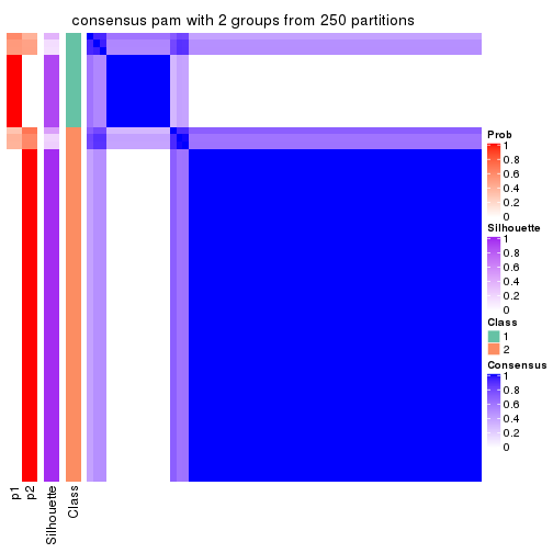
consensus_heatmap(res, k = 3)
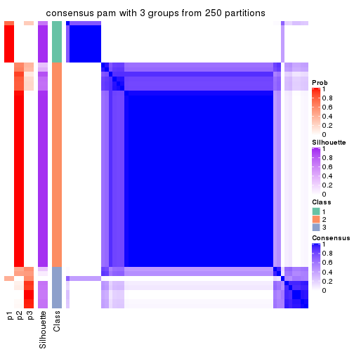
consensus_heatmap(res, k = 4)
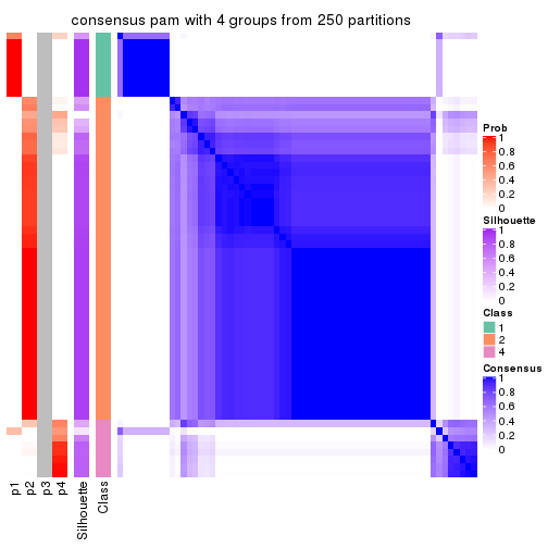
consensus_heatmap(res, k = 5)
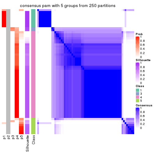
consensus_heatmap(res, k = 6)
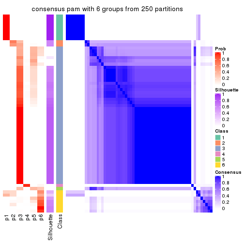
Heatmaps for the membership of samples in all partitions to see how consistent they are:
membership_heatmap(res, k = 2)
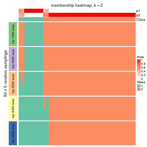
membership_heatmap(res, k = 3)
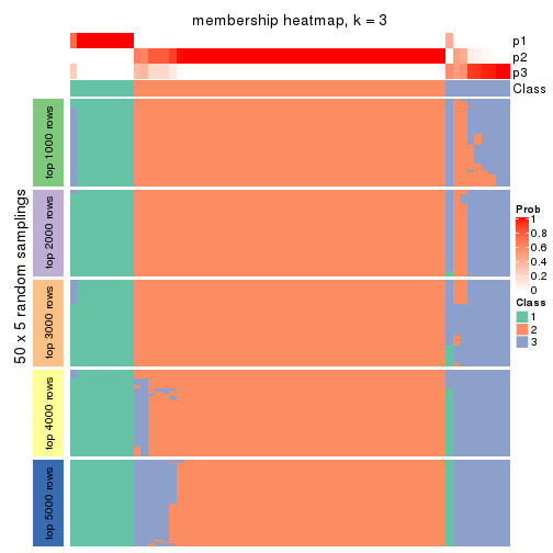
membership_heatmap(res, k = 4)
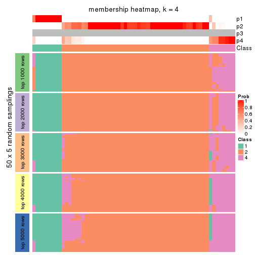
membership_heatmap(res, k = 5)
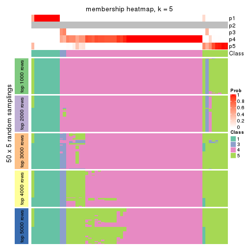
membership_heatmap(res, k = 6)
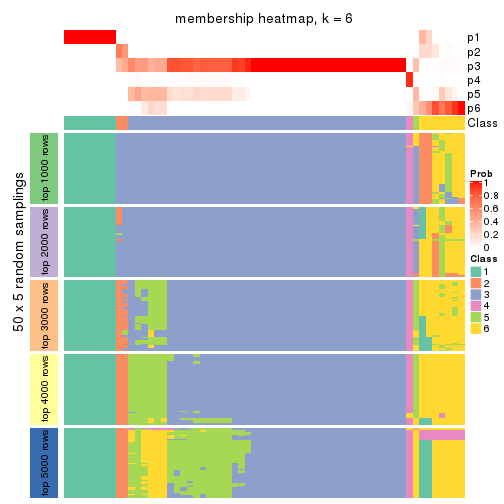
As soon as we have had the classes for columns, we can look for signatures which are significantly different between classes which can be candidate marks for certain classes. Following are the heatmaps for signatures.
Signature heatmaps where rows are scaled:
get_signatures(res, k = 2)
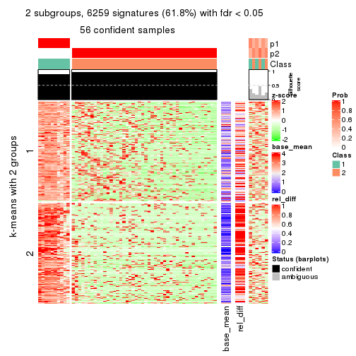
get_signatures(res, k = 3)
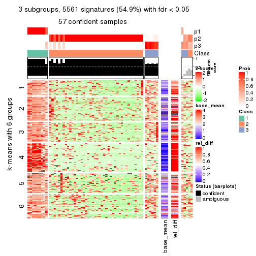
get_signatures(res, k = 4)
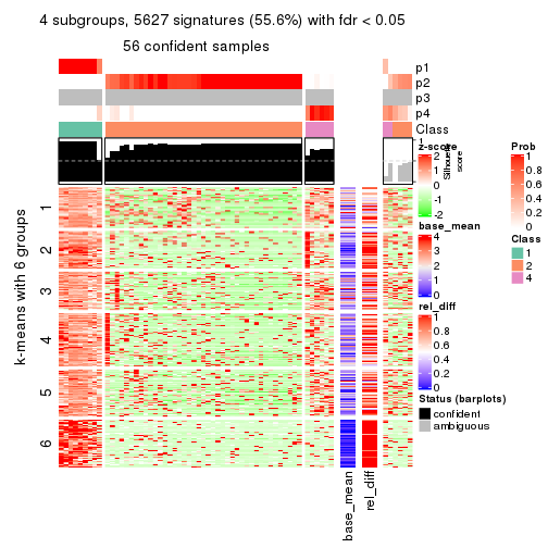
get_signatures(res, k = 5)
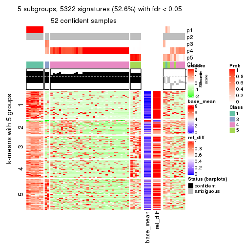
get_signatures(res, k = 6)
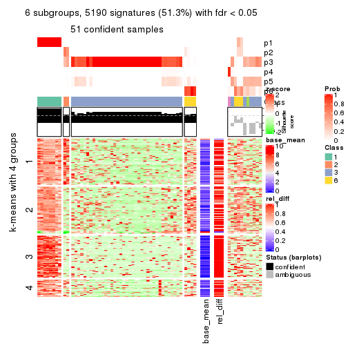
Signature heatmaps where rows are not scaled:
get_signatures(res, k = 2, scale_rows = FALSE)

get_signatures(res, k = 3, scale_rows = FALSE)
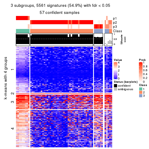
get_signatures(res, k = 4, scale_rows = FALSE)
#> Error in mat[ceiling(1:nr/h_ratio), ceiling(1:nc/w_ratio), drop = FALSE]: subscript out of bounds

get_signatures(res, k = 5, scale_rows = FALSE)
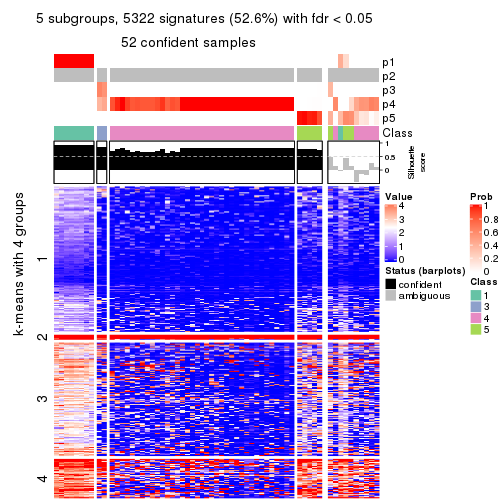
get_signatures(res, k = 6, scale_rows = FALSE)
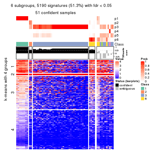
Compare the overlap of signatures from different k:
compare_signatures(res)
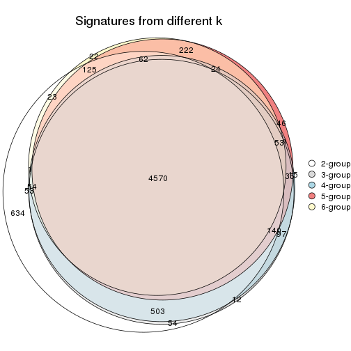
get_signature() returns a data frame invisibly. TO get the list of signatures, the function
call should be assigned to a variable explicitly. In following code, if plot argument is set
to FALSE, no heatmap is plotted while only the differential analysis is performed.
# code only for demonstration
tb = get_signature(res, k = ..., plot = FALSE)
An example of the output of tb is:
#> which_row fdr mean_1 mean_2 scaled_mean_1 scaled_mean_2 km
#> 1 38 0.042760348 8.373488 9.131774 -0.5533452 0.5164555 1
#> 2 40 0.018707592 7.106213 8.469186 -0.6173731 0.5762149 1
#> 3 55 0.019134737 10.221463 11.207825 -0.6159697 0.5749050 1
#> 4 59 0.006059896 5.921854 7.869574 -0.6899429 0.6439467 1
#> 5 60 0.018055526 8.928898 10.211722 -0.6204761 0.5791110 1
#> 6 98 0.009384629 15.714769 14.887706 0.6635654 -0.6193277 2
...
The columns in tb are:
which_row: row indices corresponding to the input matrix.fdr: FDR for the differential test. mean_x: The mean value in group x.scaled_mean_x: The mean value in group x after rows are scaled.km: Row groups if k-means clustering is applied to rows.UMAP plot which shows how samples are separated.
dimension_reduction(res, k = 2, method = "UMAP")
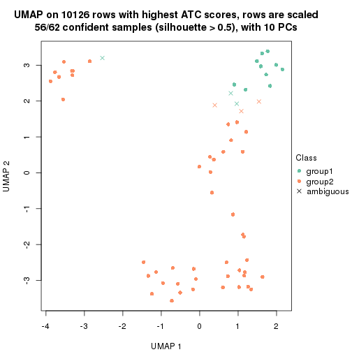
dimension_reduction(res, k = 3, method = "UMAP")
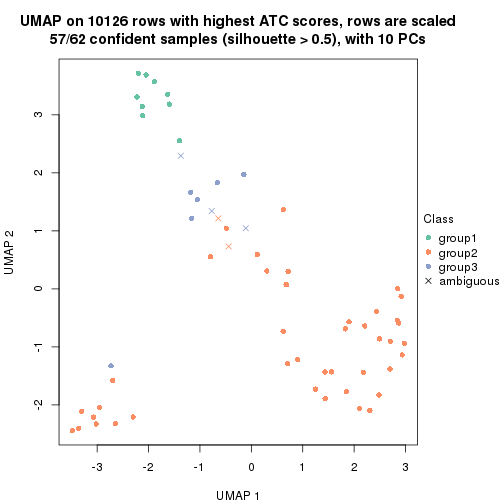
dimension_reduction(res, k = 4, method = "UMAP")
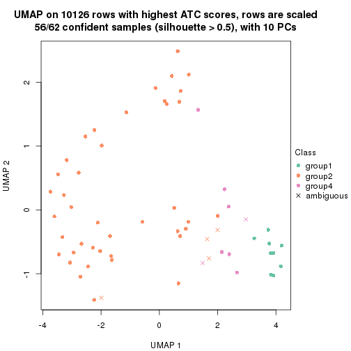
dimension_reduction(res, k = 5, method = "UMAP")
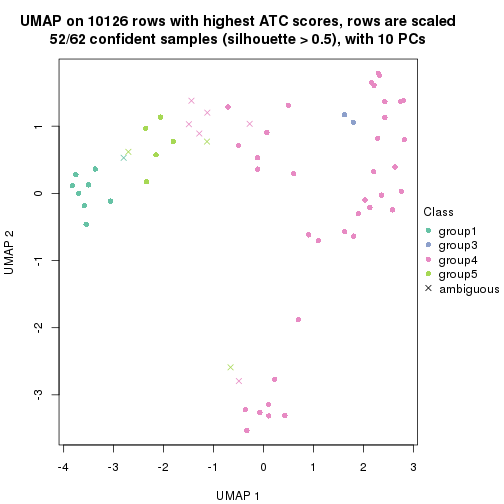
dimension_reduction(res, k = 6, method = "UMAP")
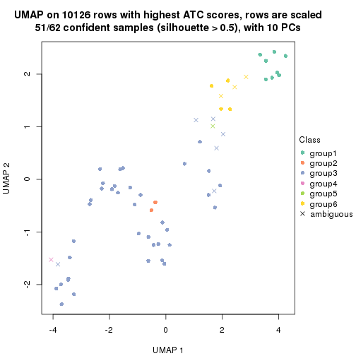
Following heatmap shows how subgroups are split when increasing k:
collect_classes(res)
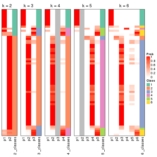
If matrix rows can be associated to genes, consider to use functional_enrichment(res,
...) to perform function enrichment for the signature genes. See this vignette for more detailed explanations.
The object with results only for a single top-value method and a single partition method can be extracted as:
res = res_list["ATC", "mclust"]
# you can also extract it by
# res = res_list["ATC:mclust"]
A summary of res and all the functions that can be applied to it:
res
#> A 'ConsensusPartition' object with k = 2, 3, 4, 5, 6.
#> On a matrix with 10126 rows and 62 columns.
#> Top rows (1000, 2000, 3000, 4000, 5000) are extracted by 'ATC' method.
#> Subgroups are detected by 'mclust' method.
#> Performed in total 1250 partitions by row resampling.
#> Best k for subgroups seems to be 3.
#>
#> Following methods can be applied to this 'ConsensusPartition' object:
#> [1] "cola_report" "collect_classes" "collect_plots"
#> [4] "collect_stats" "colnames" "compare_signatures"
#> [7] "consensus_heatmap" "dimension_reduction" "functional_enrichment"
#> [10] "get_anno_col" "get_anno" "get_classes"
#> [13] "get_consensus" "get_matrix" "get_membership"
#> [16] "get_param" "get_signatures" "get_stats"
#> [19] "is_best_k" "is_stable_k" "membership_heatmap"
#> [22] "ncol" "nrow" "plot_ecdf"
#> [25] "rownames" "select_partition_number" "show"
#> [28] "suggest_best_k" "test_to_known_factors"
collect_plots() function collects all the plots made from res for all k (number of partitions)
into one single page to provide an easy and fast comparison between different k.
collect_plots(res)
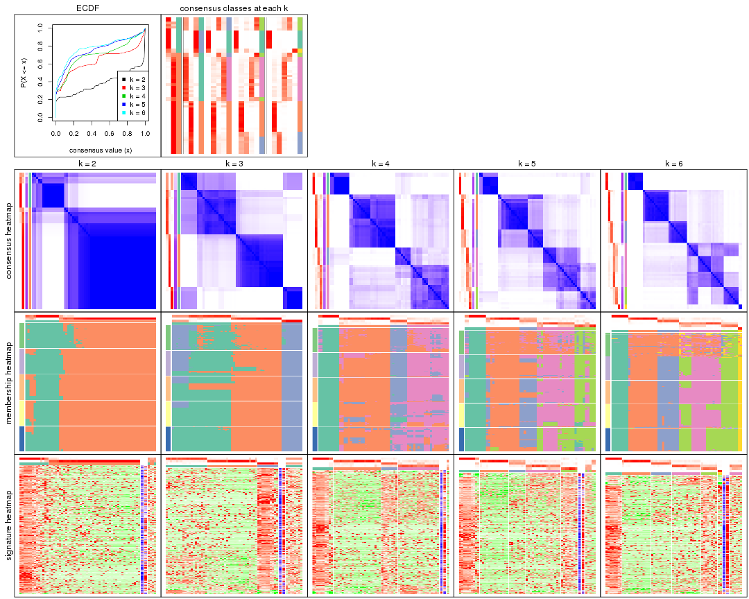
The plots are:
k and the heatmap of
predicted classes for each k.k.k.k.All the plots in panels can be made by individual functions and they are plotted later in this section.
select_partition_number() produces several plots showing different
statistics for choosing “optimized” k. There are following statistics:
k;k, the area increased is defined as \(A_k - A_{k-1}\).The detailed explanations of these statistics can be found in the cola vignette.
Generally speaking, lower PAC score, higher mean silhouette score or higher
concordance corresponds to better partition. Rand index and Jaccard index
measure how similar the current partition is compared to partition with k-1.
If they are too similar, we won't accept k is better than k-1.
select_partition_number(res)

The numeric values for all these statistics can be obtained by get_stats().
get_stats(res)
#> k 1-PAC mean_silhouette concordance area_increased Rand Jaccard
#> 2 2 0.749 0.861 0.943 0.3827 0.611 0.611
#> 3 3 0.658 0.799 0.882 0.6640 0.619 0.441
#> 4 4 0.494 0.824 0.839 0.1048 0.915 0.771
#> 5 5 0.615 0.683 0.781 0.0742 0.905 0.676
#> 6 6 0.661 0.748 0.812 0.0340 0.941 0.747
suggest_best_k() suggests the best \(k\) based on these statistics. The rules are as follows:
suggest_best_k(res)
#> [1] 3
Following shows the table of the partitions (You need to click the show/hide
code output link to see it). The membership matrix (columns with name p*)
is inferred by
clue::cl_consensus()
function with the SE method. Basically the value in the membership matrix
represents the probability to belong to a certain group. The finall class
label for an item is determined with the group with highest probability it
belongs to.
In get_classes() function, the entropy is calculated from the membership
matrix and the silhouette score is calculated from the consensus matrix.
cbind(get_classes(res, k = 2), get_membership(res, k = 2))
#> class entropy silhouette p1 p2
#> SRR764776 1 0.0000 0.874 1.000 0.000
#> SRR764777 1 0.0000 0.874 1.000 0.000
#> SRR764778 1 0.0000 0.874 1.000 0.000
#> SRR764779 1 0.0000 0.874 1.000 0.000
#> SRR764780 1 0.0000 0.874 1.000 0.000
#> SRR764781 1 0.0000 0.874 1.000 0.000
#> SRR764782 2 0.6973 0.752 0.188 0.812
#> SRR764783 2 0.9881 0.144 0.436 0.564
#> SRR764784 2 0.5294 0.840 0.120 0.880
#> SRR764785 2 0.0000 0.953 0.000 1.000
#> SRR764786 2 0.0000 0.953 0.000 1.000
#> SRR764787 2 0.0672 0.948 0.008 0.992
#> SRR764788 2 0.6973 0.752 0.188 0.812
#> SRR764789 2 0.0000 0.953 0.000 1.000
#> SRR764790 2 0.0000 0.953 0.000 1.000
#> SRR764791 2 0.2236 0.926 0.036 0.964
#> SRR764792 2 0.0000 0.953 0.000 1.000
#> SRR764793 2 0.0938 0.946 0.012 0.988
#> SRR764794 2 0.1184 0.943 0.016 0.984
#> SRR764795 2 0.6973 0.752 0.188 0.812
#> SRR764796 2 0.1843 0.934 0.028 0.972
#> SRR764797 1 0.9988 0.149 0.520 0.480
#> SRR764798 1 0.8443 0.644 0.728 0.272
#> SRR764799 1 0.0000 0.874 1.000 0.000
#> SRR764800 1 0.0000 0.874 1.000 0.000
#> SRR764801 1 0.8909 0.596 0.692 0.308
#> SRR764802 2 0.9732 0.247 0.404 0.596
#> SRR764803 1 0.7745 0.695 0.772 0.228
#> SRR764804 2 0.0000 0.953 0.000 1.000
#> SRR764805 2 0.0000 0.953 0.000 1.000
#> SRR764806 2 0.0000 0.953 0.000 1.000
#> SRR764807 2 0.0000 0.953 0.000 1.000
#> SRR764808 2 0.0000 0.953 0.000 1.000
#> SRR764809 2 0.0000 0.953 0.000 1.000
#> SRR764810 2 0.0000 0.953 0.000 1.000
#> SRR764811 2 0.0000 0.953 0.000 1.000
#> SRR764812 2 0.0000 0.953 0.000 1.000
#> SRR764813 2 0.0000 0.953 0.000 1.000
#> SRR764814 1 0.9850 0.320 0.572 0.428
#> SRR764815 2 0.1633 0.937 0.024 0.976
#> SRR764816 1 0.0000 0.874 1.000 0.000
#> SRR764817 1 0.0000 0.874 1.000 0.000
#> SRR1066622 2 0.0000 0.953 0.000 1.000
#> SRR1066623 2 0.0000 0.953 0.000 1.000
#> SRR1066624 1 0.0376 0.872 0.996 0.004
#> SRR1066625 2 0.6531 0.781 0.168 0.832
#> SRR1066626 2 0.0000 0.953 0.000 1.000
#> SRR1066627 2 0.0000 0.953 0.000 1.000
#> SRR1066628 2 0.0000 0.953 0.000 1.000
#> SRR1066629 2 0.0000 0.953 0.000 1.000
#> SRR1066630 2 0.0000 0.953 0.000 1.000
#> SRR1066631 2 0.0000 0.953 0.000 1.000
#> SRR1066632 2 0.0000 0.953 0.000 1.000
#> SRR1066633 2 0.0000 0.953 0.000 1.000
#> SRR1066634 2 0.0000 0.953 0.000 1.000
#> SRR1066635 2 0.0000 0.953 0.000 1.000
#> SRR1066636 2 0.0000 0.953 0.000 1.000
#> SRR1066637 2 0.0000 0.953 0.000 1.000
#> SRR1066638 2 0.0000 0.953 0.000 1.000
#> SRR1066639 2 0.0000 0.953 0.000 1.000
#> SRR1066640 2 0.0000 0.953 0.000 1.000
#> SRR1066641 2 0.0000 0.953 0.000 1.000
cbind(get_classes(res, k = 3), get_membership(res, k = 3))
#> class entropy silhouette p1 p2 p3
#> SRR764776 3 0.0000 0.981 0.000 0.000 1.000
#> SRR764777 3 0.0000 0.981 0.000 0.000 1.000
#> SRR764778 3 0.0000 0.981 0.000 0.000 1.000
#> SRR764779 3 0.0000 0.981 0.000 0.000 1.000
#> SRR764780 1 0.6295 0.273 0.528 0.000 0.472
#> SRR764781 1 0.6295 0.273 0.528 0.000 0.472
#> SRR764782 1 0.3899 0.779 0.888 0.056 0.056
#> SRR764783 1 0.6286 0.288 0.536 0.000 0.464
#> SRR764784 1 0.2384 0.786 0.936 0.056 0.008
#> SRR764785 2 0.4887 0.762 0.228 0.772 0.000
#> SRR764786 2 0.0592 0.951 0.012 0.988 0.000
#> SRR764787 1 0.2537 0.789 0.920 0.080 0.000
#> SRR764788 1 0.3896 0.782 0.888 0.060 0.052
#> SRR764789 1 0.3340 0.781 0.880 0.120 0.000
#> SRR764790 2 0.5254 0.680 0.264 0.736 0.000
#> SRR764791 1 0.2590 0.788 0.924 0.072 0.004
#> SRR764792 1 0.2878 0.783 0.904 0.096 0.000
#> SRR764793 1 0.2400 0.787 0.932 0.064 0.004
#> SRR764794 1 0.2356 0.787 0.928 0.072 0.000
#> SRR764795 1 0.3899 0.779 0.888 0.056 0.056
#> SRR764796 1 0.2496 0.789 0.928 0.068 0.004
#> SRR764797 1 0.6274 0.299 0.544 0.000 0.456
#> SRR764798 3 0.2165 0.927 0.064 0.000 0.936
#> SRR764799 3 0.0000 0.981 0.000 0.000 1.000
#> SRR764800 3 0.0000 0.981 0.000 0.000 1.000
#> SRR764801 3 0.2537 0.906 0.080 0.000 0.920
#> SRR764802 1 0.6280 0.294 0.540 0.000 0.460
#> SRR764803 1 0.6291 0.280 0.532 0.000 0.468
#> SRR764804 2 0.0000 0.949 0.000 1.000 0.000
#> SRR764805 2 0.0424 0.951 0.008 0.992 0.000
#> SRR764806 2 0.2711 0.920 0.088 0.912 0.000
#> SRR764807 2 0.0237 0.950 0.004 0.996 0.000
#> SRR764808 2 0.0237 0.950 0.004 0.996 0.000
#> SRR764809 2 0.0000 0.949 0.000 1.000 0.000
#> SRR764810 2 0.0000 0.949 0.000 1.000 0.000
#> SRR764811 2 0.0000 0.949 0.000 1.000 0.000
#> SRR764812 2 0.0000 0.949 0.000 1.000 0.000
#> SRR764813 2 0.0000 0.949 0.000 1.000 0.000
#> SRR764814 1 0.6308 0.223 0.508 0.000 0.492
#> SRR764815 1 0.2682 0.788 0.920 0.076 0.004
#> SRR764816 3 0.0000 0.981 0.000 0.000 1.000
#> SRR764817 3 0.0000 0.981 0.000 0.000 1.000
#> SRR1066622 1 0.3116 0.785 0.892 0.108 0.000
#> SRR1066623 1 0.3192 0.784 0.888 0.112 0.000
#> SRR1066624 1 0.6302 0.255 0.520 0.000 0.480
#> SRR1066625 1 0.5253 0.756 0.828 0.076 0.096
#> SRR1066626 1 0.4121 0.756 0.832 0.168 0.000
#> SRR1066627 1 0.2625 0.789 0.916 0.084 0.000
#> SRR1066628 1 0.4750 0.718 0.784 0.216 0.000
#> SRR1066629 1 0.2878 0.788 0.904 0.096 0.000
#> SRR1066630 2 0.0592 0.950 0.012 0.988 0.000
#> SRR1066631 1 0.4750 0.717 0.784 0.216 0.000
#> SRR1066632 2 0.3816 0.866 0.148 0.852 0.000
#> SRR1066633 2 0.2448 0.929 0.076 0.924 0.000
#> SRR1066634 2 0.1860 0.944 0.052 0.948 0.000
#> SRR1066635 2 0.1643 0.947 0.044 0.956 0.000
#> SRR1066636 2 0.1529 0.947 0.040 0.960 0.000
#> SRR1066637 2 0.1753 0.945 0.048 0.952 0.000
#> SRR1066638 2 0.1964 0.943 0.056 0.944 0.000
#> SRR1066639 2 0.1529 0.948 0.040 0.960 0.000
#> SRR1066640 2 0.1529 0.947 0.040 0.960 0.000
#> SRR1066641 2 0.0000 0.949 0.000 1.000 0.000
cbind(get_classes(res, k = 4), get_membership(res, k = 4))
#> class entropy silhouette p1 p2 p3 p4
#> SRR764776 1 0.0000 0.959 1.000 0.000 0.000 0.000
#> SRR764777 1 0.0000 0.959 1.000 0.000 0.000 0.000
#> SRR764778 1 0.0000 0.959 1.000 0.000 0.000 0.000
#> SRR764779 1 0.0000 0.959 1.000 0.000 0.000 0.000
#> SRR764780 3 0.4462 0.907 0.064 0.000 0.804 0.132
#> SRR764781 3 0.4388 0.907 0.060 0.000 0.808 0.132
#> SRR764782 4 0.6663 0.634 0.000 0.124 0.280 0.596
#> SRR764783 3 0.4532 0.883 0.052 0.000 0.792 0.156
#> SRR764784 4 0.6265 0.702 0.000 0.124 0.220 0.656
#> SRR764785 2 0.5732 0.592 0.000 0.672 0.064 0.264
#> SRR764786 2 0.1938 0.871 0.000 0.936 0.012 0.052
#> SRR764787 4 0.4735 0.794 0.000 0.148 0.068 0.784
#> SRR764788 4 0.6319 0.587 0.000 0.084 0.312 0.604
#> SRR764789 4 0.4716 0.786 0.000 0.196 0.040 0.764
#> SRR764790 2 0.5839 0.457 0.000 0.648 0.060 0.292
#> SRR764791 4 0.3978 0.791 0.000 0.108 0.056 0.836
#> SRR764792 4 0.4920 0.752 0.000 0.136 0.088 0.776
#> SRR764793 4 0.3521 0.791 0.000 0.084 0.052 0.864
#> SRR764794 4 0.4780 0.725 0.000 0.116 0.096 0.788
#> SRR764795 4 0.6592 0.622 0.000 0.116 0.284 0.600
#> SRR764796 4 0.5628 0.765 0.000 0.132 0.144 0.724
#> SRR764797 3 0.5201 0.903 0.064 0.004 0.752 0.180
#> SRR764798 1 0.4300 0.809 0.820 0.000 0.092 0.088
#> SRR764799 1 0.0000 0.959 1.000 0.000 0.000 0.000
#> SRR764800 1 0.0000 0.959 1.000 0.000 0.000 0.000
#> SRR764801 1 0.4300 0.808 0.820 0.000 0.092 0.088
#> SRR764802 3 0.5239 0.861 0.048 0.016 0.760 0.176
#> SRR764803 3 0.4364 0.906 0.056 0.000 0.808 0.136
#> SRR764804 2 0.0469 0.883 0.000 0.988 0.012 0.000
#> SRR764805 2 0.0469 0.885 0.000 0.988 0.000 0.012
#> SRR764806 2 0.4581 0.838 0.000 0.800 0.120 0.080
#> SRR764807 2 0.1854 0.866 0.000 0.940 0.012 0.048
#> SRR764808 2 0.0804 0.884 0.000 0.980 0.012 0.008
#> SRR764809 2 0.0000 0.884 0.000 1.000 0.000 0.000
#> SRR764810 2 0.0188 0.885 0.000 0.996 0.000 0.004
#> SRR764811 2 0.0657 0.884 0.000 0.984 0.012 0.004
#> SRR764812 2 0.0469 0.883 0.000 0.988 0.012 0.000
#> SRR764813 2 0.0469 0.883 0.000 0.988 0.012 0.000
#> SRR764814 3 0.5562 0.865 0.124 0.004 0.740 0.132
#> SRR764815 4 0.4362 0.734 0.000 0.096 0.088 0.816
#> SRR764816 1 0.0000 0.959 1.000 0.000 0.000 0.000
#> SRR764817 1 0.0000 0.959 1.000 0.000 0.000 0.000
#> SRR1066622 4 0.3674 0.783 0.000 0.116 0.036 0.848
#> SRR1066623 4 0.3895 0.780 0.000 0.132 0.036 0.832
#> SRR1066624 3 0.5000 0.894 0.100 0.000 0.772 0.128
#> SRR1066625 4 0.4568 0.570 0.004 0.024 0.200 0.772
#> SRR1066626 4 0.5025 0.741 0.000 0.252 0.032 0.716
#> SRR1066627 4 0.3497 0.782 0.000 0.104 0.036 0.860
#> SRR1066628 4 0.4818 0.737 0.000 0.216 0.036 0.748
#> SRR1066629 4 0.3694 0.791 0.000 0.124 0.032 0.844
#> SRR1066630 2 0.2635 0.842 0.000 0.904 0.020 0.076
#> SRR1066631 4 0.5074 0.741 0.000 0.236 0.040 0.724
#> SRR1066632 2 0.5330 0.793 0.000 0.748 0.120 0.132
#> SRR1066633 2 0.3833 0.864 0.000 0.848 0.080 0.072
#> SRR1066634 2 0.4301 0.849 0.000 0.816 0.120 0.064
#> SRR1066635 2 0.2363 0.877 0.000 0.920 0.024 0.056
#> SRR1066636 2 0.4150 0.853 0.000 0.824 0.120 0.056
#> SRR1066637 2 0.3991 0.854 0.000 0.832 0.120 0.048
#> SRR1066638 2 0.4227 0.850 0.000 0.820 0.120 0.060
#> SRR1066639 2 0.3679 0.866 0.000 0.856 0.084 0.060
#> SRR1066640 2 0.3991 0.854 0.000 0.832 0.120 0.048
#> SRR1066641 2 0.0657 0.881 0.000 0.984 0.012 0.004
cbind(get_classes(res, k = 5), get_membership(res, k = 5))
#> class entropy silhouette p1 p2 p3 p4 p5
#> SRR764776 1 0.0162 0.919 0.996 0.000 0.004 0.000 0.000
#> SRR764777 1 0.0162 0.919 0.996 0.000 0.004 0.000 0.000
#> SRR764778 1 0.0162 0.919 0.996 0.000 0.004 0.000 0.000
#> SRR764779 1 0.0162 0.919 0.996 0.000 0.004 0.000 0.000
#> SRR764780 5 0.3450 0.705 0.096 0.000 0.044 0.012 0.848
#> SRR764781 5 0.3340 0.712 0.088 0.000 0.044 0.012 0.856
#> SRR764782 4 0.5779 0.385 0.000 0.032 0.032 0.488 0.448
#> SRR764783 5 0.0613 0.709 0.000 0.004 0.008 0.004 0.984
#> SRR764784 4 0.6645 0.515 0.000 0.064 0.064 0.488 0.384
#> SRR764785 2 0.4456 0.629 0.000 0.792 0.080 0.100 0.028
#> SRR764786 2 0.1806 0.802 0.000 0.940 0.016 0.016 0.028
#> SRR764787 4 0.5637 0.700 0.000 0.068 0.024 0.644 0.264
#> SRR764788 5 0.6231 -0.357 0.000 0.056 0.040 0.404 0.500
#> SRR764789 4 0.6289 0.707 0.000 0.108 0.040 0.612 0.240
#> SRR764790 2 0.3129 0.711 0.000 0.872 0.020 0.076 0.032
#> SRR764791 4 0.6215 0.715 0.000 0.088 0.048 0.620 0.244
#> SRR764792 4 0.5854 0.717 0.000 0.100 0.024 0.644 0.232
#> SRR764793 4 0.5682 0.714 0.000 0.088 0.016 0.640 0.256
#> SRR764794 4 0.6075 0.705 0.000 0.072 0.068 0.652 0.208
#> SRR764795 5 0.5972 -0.393 0.000 0.040 0.036 0.444 0.480
#> SRR764796 4 0.5652 0.629 0.000 0.040 0.036 0.616 0.308
#> SRR764797 5 0.5296 0.695 0.076 0.004 0.152 0.036 0.732
#> SRR764798 1 0.6113 0.614 0.592 0.024 0.316 0.052 0.016
#> SRR764799 1 0.0162 0.919 0.996 0.000 0.004 0.000 0.000
#> SRR764800 1 0.0162 0.919 0.996 0.000 0.004 0.000 0.000
#> SRR764801 1 0.6095 0.614 0.592 0.012 0.312 0.064 0.020
#> SRR764802 5 0.1503 0.696 0.000 0.020 0.020 0.008 0.952
#> SRR764803 5 0.1697 0.717 0.000 0.000 0.060 0.008 0.932
#> SRR764804 2 0.0162 0.836 0.000 0.996 0.004 0.000 0.000
#> SRR764805 2 0.0693 0.828 0.000 0.980 0.012 0.008 0.000
#> SRR764806 3 0.5707 0.899 0.000 0.364 0.544 0.092 0.000
#> SRR764807 2 0.0510 0.830 0.000 0.984 0.016 0.000 0.000
#> SRR764808 2 0.0162 0.836 0.000 0.996 0.000 0.004 0.000
#> SRR764809 2 0.0566 0.831 0.000 0.984 0.012 0.004 0.000
#> SRR764810 2 0.0566 0.831 0.000 0.984 0.012 0.004 0.000
#> SRR764811 2 0.0324 0.835 0.000 0.992 0.004 0.004 0.000
#> SRR764812 2 0.0000 0.837 0.000 1.000 0.000 0.000 0.000
#> SRR764813 2 0.0000 0.837 0.000 1.000 0.000 0.000 0.000
#> SRR764814 5 0.4769 0.608 0.156 0.004 0.060 0.020 0.760
#> SRR764815 4 0.5974 0.705 0.000 0.064 0.056 0.644 0.236
#> SRR764816 1 0.0162 0.919 0.996 0.000 0.004 0.000 0.000
#> SRR764817 1 0.0162 0.919 0.996 0.000 0.004 0.000 0.000
#> SRR1066622 4 0.2130 0.695 0.000 0.080 0.012 0.908 0.000
#> SRR1066623 4 0.2069 0.695 0.000 0.076 0.012 0.912 0.000
#> SRR1066624 5 0.5484 0.643 0.068 0.000 0.164 0.056 0.712
#> SRR1066625 4 0.6035 0.568 0.000 0.032 0.092 0.624 0.252
#> SRR1066626 4 0.2806 0.679 0.000 0.152 0.004 0.844 0.000
#> SRR1066627 4 0.1830 0.694 0.000 0.068 0.008 0.924 0.000
#> SRR1066628 4 0.3224 0.668 0.000 0.160 0.016 0.824 0.000
#> SRR1066629 4 0.2361 0.697 0.000 0.096 0.012 0.892 0.000
#> SRR1066630 2 0.1904 0.792 0.000 0.936 0.016 0.020 0.028
#> SRR1066631 4 0.3340 0.675 0.000 0.156 0.016 0.824 0.004
#> SRR1066632 3 0.6022 0.845 0.000 0.324 0.540 0.136 0.000
#> SRR1066633 3 0.5768 0.847 0.000 0.428 0.484 0.088 0.000
#> SRR1066634 3 0.5447 0.925 0.000 0.400 0.536 0.064 0.000
#> SRR1066635 2 0.5261 -0.693 0.000 0.528 0.424 0.048 0.000
#> SRR1066636 3 0.5447 0.927 0.000 0.400 0.536 0.064 0.000
#> SRR1066637 3 0.5071 0.909 0.000 0.424 0.540 0.036 0.000
#> SRR1066638 3 0.5535 0.926 0.000 0.392 0.536 0.072 0.000
#> SRR1066639 2 0.5281 -0.624 0.000 0.548 0.400 0.052 0.000
#> SRR1066640 3 0.5302 0.920 0.000 0.412 0.536 0.052 0.000
#> SRR1066641 2 0.0324 0.835 0.000 0.992 0.004 0.004 0.000
cbind(get_classes(res, k = 6), get_membership(res, k = 6))
#> class entropy silhouette p1 p2 p3 p4 p5 p6
#> SRR764776 1 0.0000 0.9933 1.000 0.000 0.000 0.000 0.000 0.000
#> SRR764777 1 0.0000 0.9933 1.000 0.000 0.000 0.000 0.000 0.000
#> SRR764778 1 0.0000 0.9933 1.000 0.000 0.000 0.000 0.000 0.000
#> SRR764779 1 0.0000 0.9933 1.000 0.000 0.000 0.000 0.000 0.000
#> SRR764780 5 0.3946 0.9198 0.000 0.000 0.020 0.228 0.736 0.016
#> SRR764781 5 0.3541 0.9204 0.000 0.000 0.020 0.232 0.748 0.000
#> SRR764782 4 0.5151 -0.2982 0.000 0.024 0.016 0.532 0.412 0.016
#> SRR764783 5 0.3806 0.9199 0.000 0.008 0.004 0.240 0.736 0.012
#> SRR764784 4 0.5536 -0.2003 0.000 0.064 0.008 0.544 0.364 0.020
#> SRR764785 2 0.4176 0.5974 0.000 0.720 0.212 0.068 0.000 0.000
#> SRR764786 2 0.0725 0.9536 0.000 0.976 0.012 0.012 0.000 0.000
#> SRR764787 4 0.2814 0.6101 0.000 0.088 0.016 0.872 0.016 0.008
#> SRR764788 4 0.5224 -0.3447 0.000 0.032 0.012 0.508 0.432 0.016
#> SRR764789 4 0.3088 0.6127 0.000 0.120 0.048 0.832 0.000 0.000
#> SRR764790 2 0.1594 0.9076 0.000 0.932 0.016 0.052 0.000 0.000
#> SRR764791 4 0.2382 0.6076 0.000 0.072 0.008 0.896 0.004 0.020
#> SRR764792 4 0.2900 0.6174 0.000 0.112 0.016 0.856 0.012 0.004
#> SRR764793 4 0.3419 0.5702 0.000 0.096 0.008 0.824 0.072 0.000
#> SRR764794 4 0.3119 0.6072 0.000 0.080 0.020 0.860 0.008 0.032
#> SRR764795 4 0.5207 -0.2872 0.000 0.028 0.012 0.532 0.408 0.020
#> SRR764796 4 0.5153 0.0332 0.000 0.072 0.008 0.596 0.320 0.004
#> SRR764797 5 0.5600 0.8764 0.000 0.000 0.048 0.276 0.600 0.076
#> SRR764798 6 0.1036 0.9824 0.000 0.008 0.004 0.024 0.000 0.964
#> SRR764799 1 0.0405 0.9925 0.988 0.000 0.008 0.000 0.000 0.004
#> SRR764800 1 0.0508 0.9914 0.984 0.000 0.012 0.000 0.000 0.004
#> SRR764801 6 0.1148 0.9824 0.000 0.016 0.004 0.020 0.000 0.960
#> SRR764802 5 0.4778 0.8953 0.000 0.016 0.016 0.272 0.668 0.028
#> SRR764803 5 0.4914 0.9192 0.000 0.004 0.020 0.244 0.672 0.060
#> SRR764804 2 0.0260 0.9575 0.000 0.992 0.000 0.008 0.000 0.000
#> SRR764805 2 0.0508 0.9532 0.000 0.984 0.012 0.004 0.000 0.000
#> SRR764806 3 0.3621 0.9052 0.000 0.148 0.796 0.048 0.000 0.008
#> SRR764807 2 0.0603 0.9520 0.000 0.980 0.004 0.016 0.000 0.000
#> SRR764808 2 0.0146 0.9582 0.000 0.996 0.000 0.004 0.000 0.000
#> SRR764809 2 0.0146 0.9577 0.000 0.996 0.004 0.000 0.000 0.000
#> SRR764810 2 0.0291 0.9576 0.000 0.992 0.004 0.004 0.000 0.000
#> SRR764811 2 0.0291 0.9570 0.000 0.992 0.004 0.004 0.000 0.000
#> SRR764812 2 0.0260 0.9557 0.000 0.992 0.000 0.008 0.000 0.000
#> SRR764813 2 0.0146 0.9579 0.000 0.996 0.000 0.004 0.000 0.000
#> SRR764814 5 0.4537 0.9172 0.000 0.000 0.008 0.248 0.684 0.060
#> SRR764815 4 0.2920 0.6117 0.000 0.092 0.008 0.864 0.008 0.028
#> SRR764816 1 0.0508 0.9914 0.984 0.000 0.012 0.000 0.000 0.004
#> SRR764817 1 0.0363 0.9924 0.988 0.000 0.012 0.000 0.000 0.000
#> SRR1066622 4 0.5456 0.5608 0.000 0.108 0.032 0.632 0.228 0.000
#> SRR1066623 4 0.5459 0.5471 0.000 0.072 0.036 0.652 0.228 0.012
#> SRR1066624 5 0.6079 0.8670 0.000 0.000 0.140 0.236 0.572 0.052
#> SRR1066625 4 0.5289 0.3102 0.000 0.020 0.024 0.688 0.180 0.088
#> SRR1066626 4 0.5741 0.5508 0.000 0.132 0.036 0.604 0.228 0.000
#> SRR1066627 4 0.5219 0.5585 0.000 0.076 0.032 0.664 0.224 0.004
#> SRR1066628 4 0.5839 0.5431 0.000 0.144 0.036 0.592 0.228 0.000
#> SRR1066629 4 0.5502 0.5639 0.000 0.120 0.028 0.624 0.228 0.000
#> SRR1066630 2 0.0972 0.9455 0.000 0.964 0.008 0.028 0.000 0.000
#> SRR1066631 4 0.5774 0.5539 0.000 0.136 0.036 0.600 0.228 0.000
#> SRR1066632 3 0.3664 0.8538 0.000 0.108 0.804 0.080 0.000 0.008
#> SRR1066633 3 0.3141 0.9293 0.000 0.200 0.788 0.012 0.000 0.000
#> SRR1066634 3 0.3236 0.9263 0.000 0.180 0.796 0.024 0.000 0.000
#> SRR1066635 3 0.4144 0.7032 0.000 0.360 0.620 0.020 0.000 0.000
#> SRR1066636 3 0.3110 0.9324 0.000 0.196 0.792 0.012 0.000 0.000
#> SRR1066637 3 0.3345 0.9292 0.000 0.184 0.788 0.028 0.000 0.000
#> SRR1066638 3 0.3078 0.9322 0.000 0.192 0.796 0.012 0.000 0.000
#> SRR1066639 3 0.3420 0.9020 0.000 0.240 0.748 0.012 0.000 0.000
#> SRR1066640 3 0.3073 0.9312 0.000 0.204 0.788 0.008 0.000 0.000
#> SRR1066641 2 0.0458 0.9545 0.000 0.984 0.000 0.016 0.000 0.000
Heatmaps for the consensus matrix. It visualizes the probability of two samples to be in a same group.
consensus_heatmap(res, k = 2)
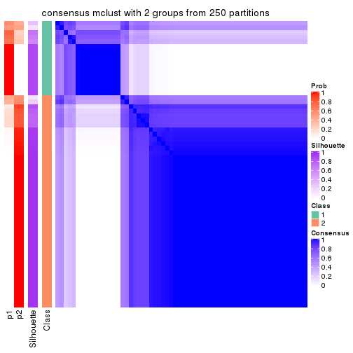
consensus_heatmap(res, k = 3)
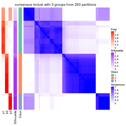
consensus_heatmap(res, k = 4)
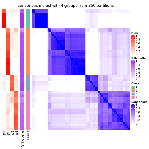
consensus_heatmap(res, k = 5)
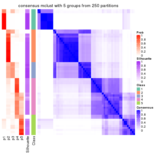
consensus_heatmap(res, k = 6)
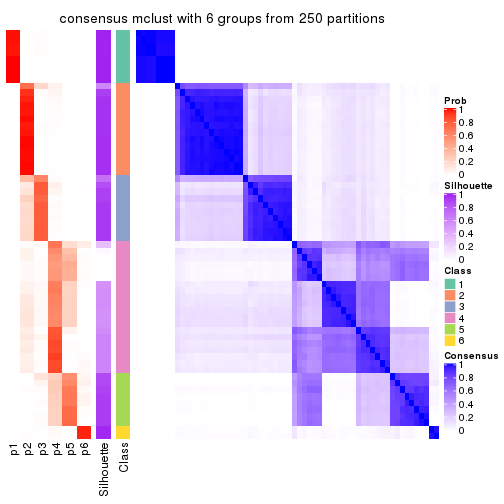
Heatmaps for the membership of samples in all partitions to see how consistent they are:
membership_heatmap(res, k = 2)
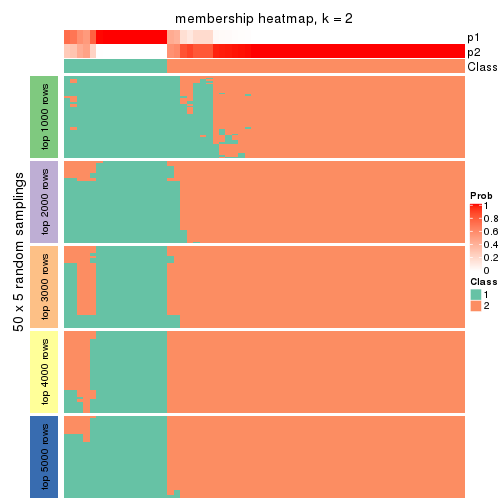
membership_heatmap(res, k = 3)
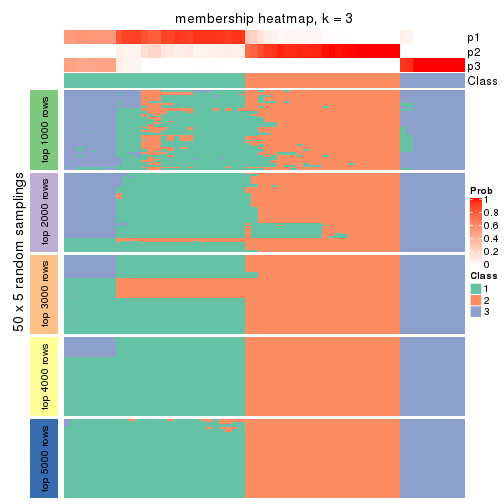
membership_heatmap(res, k = 4)
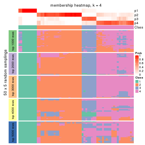
membership_heatmap(res, k = 5)
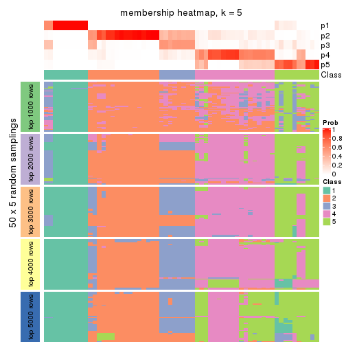
membership_heatmap(res, k = 6)
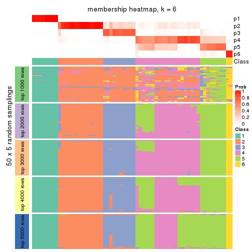
As soon as we have had the classes for columns, we can look for signatures which are significantly different between classes which can be candidate marks for certain classes. Following are the heatmaps for signatures.
Signature heatmaps where rows are scaled:
get_signatures(res, k = 2)
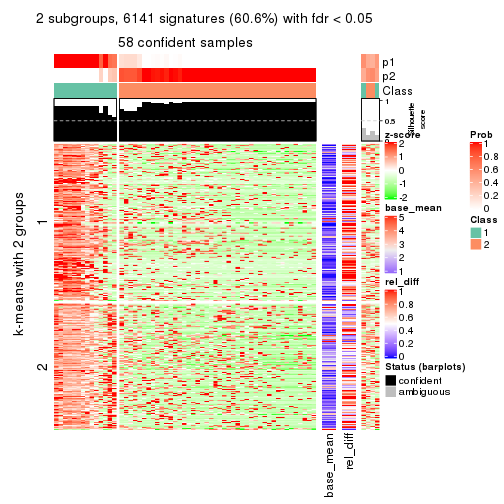
get_signatures(res, k = 3)
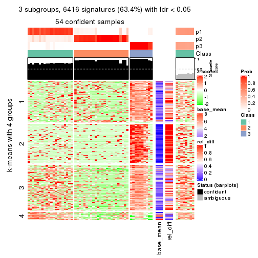
get_signatures(res, k = 4)
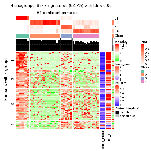
get_signatures(res, k = 5)
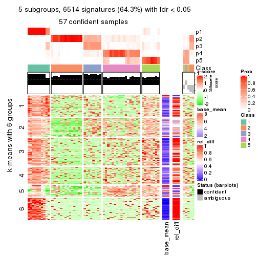
get_signatures(res, k = 6)
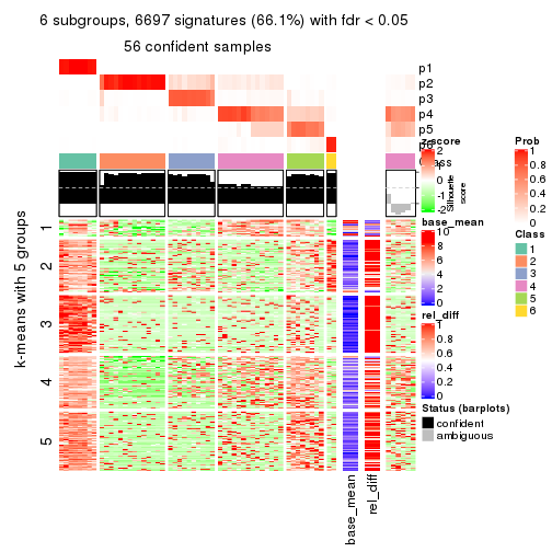
Signature heatmaps where rows are not scaled:
get_signatures(res, k = 2, scale_rows = FALSE)
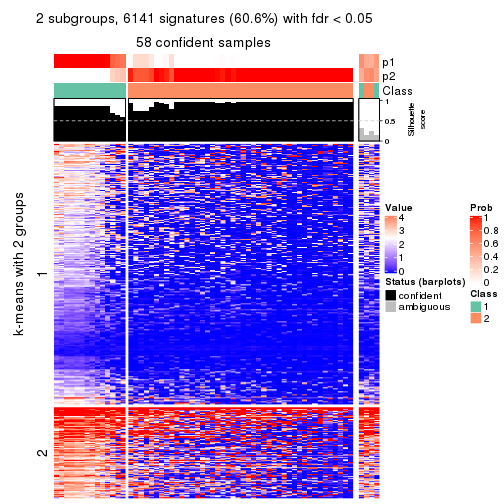
get_signatures(res, k = 3, scale_rows = FALSE)
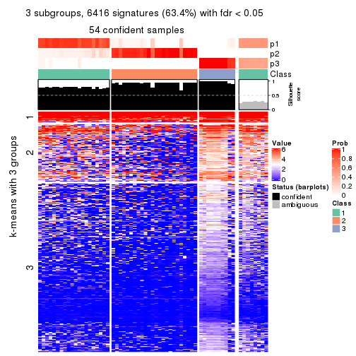
get_signatures(res, k = 4, scale_rows = FALSE)
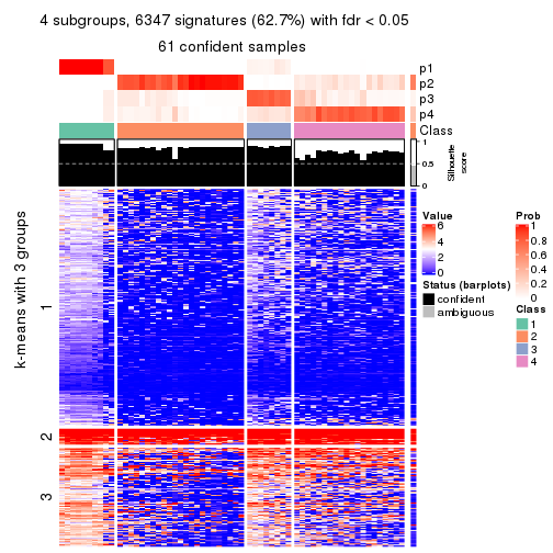
get_signatures(res, k = 5, scale_rows = FALSE)
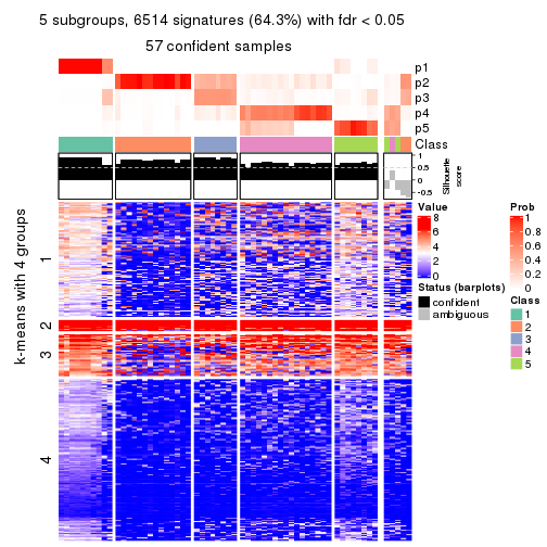
get_signatures(res, k = 6, scale_rows = FALSE)
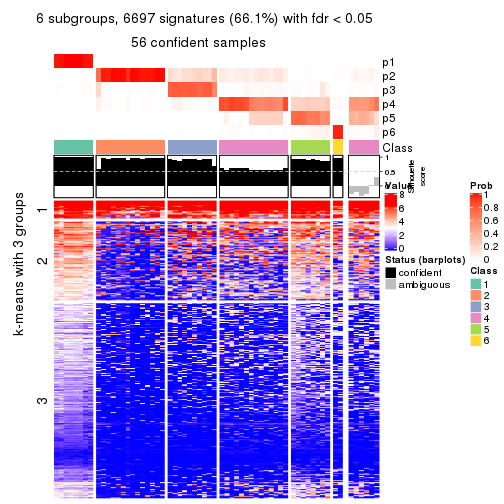
Compare the overlap of signatures from different k:
compare_signatures(res)
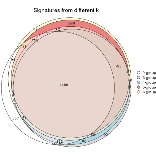
get_signature() returns a data frame invisibly. TO get the list of signatures, the function
call should be assigned to a variable explicitly. In following code, if plot argument is set
to FALSE, no heatmap is plotted while only the differential analysis is performed.
# code only for demonstration
tb = get_signature(res, k = ..., plot = FALSE)
An example of the output of tb is:
#> which_row fdr mean_1 mean_2 scaled_mean_1 scaled_mean_2 km
#> 1 38 0.042760348 8.373488 9.131774 -0.5533452 0.5164555 1
#> 2 40 0.018707592 7.106213 8.469186 -0.6173731 0.5762149 1
#> 3 55 0.019134737 10.221463 11.207825 -0.6159697 0.5749050 1
#> 4 59 0.006059896 5.921854 7.869574 -0.6899429 0.6439467 1
#> 5 60 0.018055526 8.928898 10.211722 -0.6204761 0.5791110 1
#> 6 98 0.009384629 15.714769 14.887706 0.6635654 -0.6193277 2
...
The columns in tb are:
which_row: row indices corresponding to the input matrix.fdr: FDR for the differential test. mean_x: The mean value in group x.scaled_mean_x: The mean value in group x after rows are scaled.km: Row groups if k-means clustering is applied to rows.UMAP plot which shows how samples are separated.
dimension_reduction(res, k = 2, method = "UMAP")
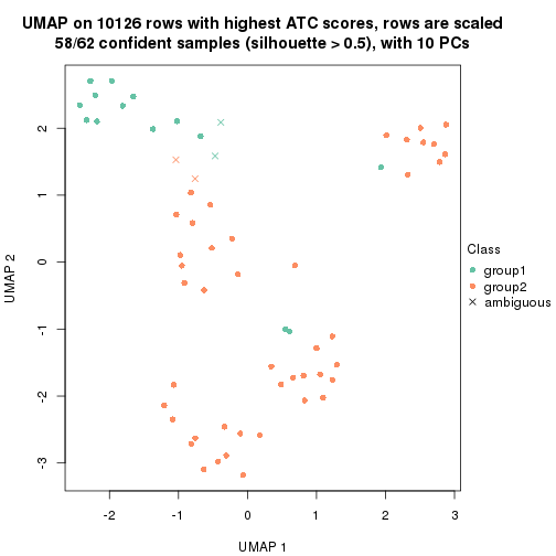
dimension_reduction(res, k = 3, method = "UMAP")

dimension_reduction(res, k = 4, method = "UMAP")
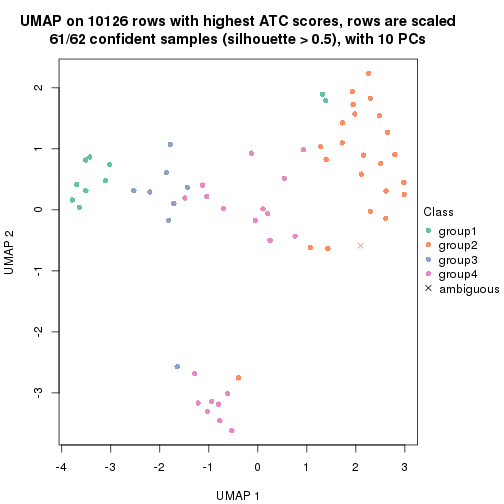
dimension_reduction(res, k = 5, method = "UMAP")
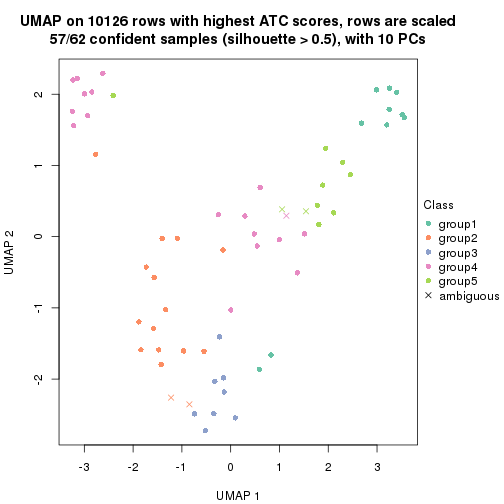
dimension_reduction(res, k = 6, method = "UMAP")
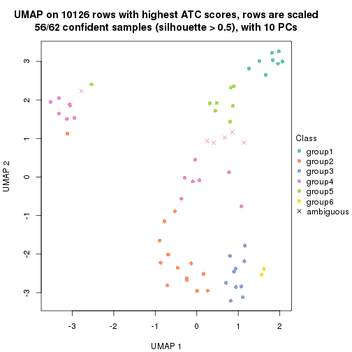
Following heatmap shows how subgroups are split when increasing k:
collect_classes(res)
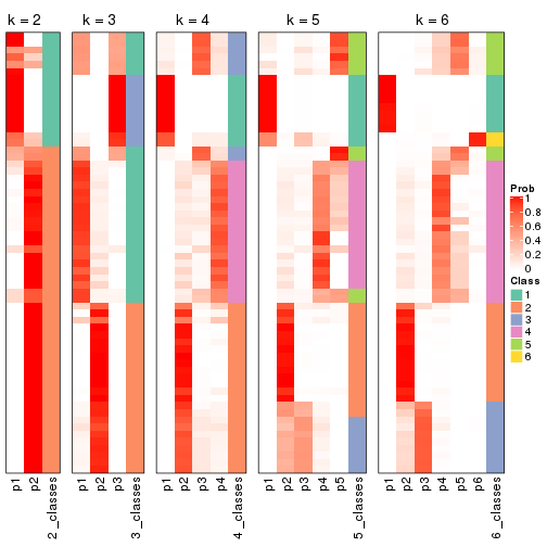
If matrix rows can be associated to genes, consider to use functional_enrichment(res,
...) to perform function enrichment for the signature genes. See this vignette for more detailed explanations.
The object with results only for a single top-value method and a single partition method can be extracted as:
res = res_list["ATC", "NMF"]
# you can also extract it by
# res = res_list["ATC:NMF"]
A summary of res and all the functions that can be applied to it:
res
#> A 'ConsensusPartition' object with k = 2, 3, 4, 5, 6.
#> On a matrix with 10126 rows and 62 columns.
#> Top rows (1000, 2000, 3000, 4000, 5000) are extracted by 'ATC' method.
#> Subgroups are detected by 'NMF' method.
#> Performed in total 1250 partitions by row resampling.
#> Best k for subgroups seems to be 3.
#>
#> Following methods can be applied to this 'ConsensusPartition' object:
#> [1] "cola_report" "collect_classes" "collect_plots"
#> [4] "collect_stats" "colnames" "compare_signatures"
#> [7] "consensus_heatmap" "dimension_reduction" "functional_enrichment"
#> [10] "get_anno_col" "get_anno" "get_classes"
#> [13] "get_consensus" "get_matrix" "get_membership"
#> [16] "get_param" "get_signatures" "get_stats"
#> [19] "is_best_k" "is_stable_k" "membership_heatmap"
#> [22] "ncol" "nrow" "plot_ecdf"
#> [25] "rownames" "select_partition_number" "show"
#> [28] "suggest_best_k" "test_to_known_factors"
collect_plots() function collects all the plots made from res for all k (number of partitions)
into one single page to provide an easy and fast comparison between different k.
collect_plots(res)
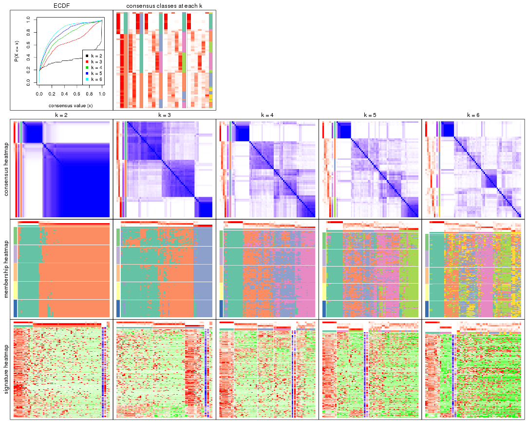
The plots are:
k and the heatmap of
predicted classes for each k.k.k.k.All the plots in panels can be made by individual functions and they are plotted later in this section.
select_partition_number() produces several plots showing different
statistics for choosing “optimized” k. There are following statistics:
k;k, the area increased is defined as \(A_k - A_{k-1}\).The detailed explanations of these statistics can be found in the cola vignette.
Generally speaking, lower PAC score, higher mean silhouette score or higher
concordance corresponds to better partition. Rand index and Jaccard index
measure how similar the current partition is compared to partition with k-1.
If they are too similar, we won't accept k is better than k-1.
select_partition_number(res)
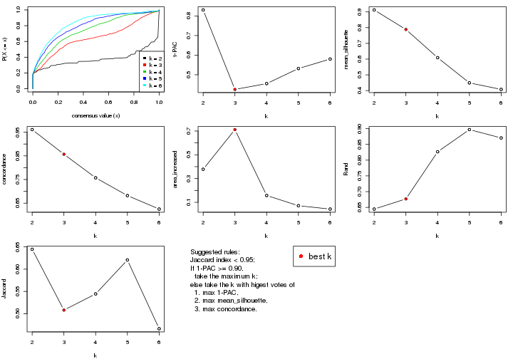
The numeric values for all these statistics can be obtained by get_stats().
get_stats(res)
#> k 1-PAC mean_silhouette concordance area_increased Rand Jaccard
#> 2 2 0.831 0.912 0.961 0.3781 0.645 0.645
#> 3 3 0.425 0.788 0.857 0.7118 0.677 0.508
#> 4 4 0.455 0.609 0.757 0.1573 0.827 0.544
#> 5 5 0.532 0.449 0.682 0.0712 0.897 0.621
#> 6 6 0.580 0.408 0.625 0.0430 0.870 0.466
suggest_best_k() suggests the best \(k\) based on these statistics. The rules are as follows:
suggest_best_k(res)
#> [1] 3
Following shows the table of the partitions (You need to click the show/hide
code output link to see it). The membership matrix (columns with name p*)
is inferred by
clue::cl_consensus()
function with the SE method. Basically the value in the membership matrix
represents the probability to belong to a certain group. The finall class
label for an item is determined with the group with highest probability it
belongs to.
In get_classes() function, the entropy is calculated from the membership
matrix and the silhouette score is calculated from the consensus matrix.
cbind(get_classes(res, k = 2), get_membership(res, k = 2))
#> class entropy silhouette p1 p2
#> SRR764776 1 0.0000 0.957 1.000 0.000
#> SRR764777 1 0.0000 0.957 1.000 0.000
#> SRR764778 1 0.0000 0.957 1.000 0.000
#> SRR764779 1 0.0000 0.957 1.000 0.000
#> SRR764780 1 0.0000 0.957 1.000 0.000
#> SRR764781 1 0.0376 0.954 0.996 0.004
#> SRR764782 2 0.0000 0.958 0.000 1.000
#> SRR764783 2 0.0000 0.958 0.000 1.000
#> SRR764784 2 0.0000 0.958 0.000 1.000
#> SRR764785 2 0.5178 0.864 0.116 0.884
#> SRR764786 2 0.0376 0.955 0.004 0.996
#> SRR764787 2 0.0000 0.958 0.000 1.000
#> SRR764788 2 0.0000 0.958 0.000 1.000
#> SRR764789 2 0.0000 0.958 0.000 1.000
#> SRR764790 1 0.0000 0.957 1.000 0.000
#> SRR764791 2 0.0000 0.958 0.000 1.000
#> SRR764792 2 0.0000 0.958 0.000 1.000
#> SRR764793 2 0.0000 0.958 0.000 1.000
#> SRR764794 2 0.0000 0.958 0.000 1.000
#> SRR764795 2 0.0000 0.958 0.000 1.000
#> SRR764796 2 0.0000 0.958 0.000 1.000
#> SRR764797 2 0.5737 0.834 0.136 0.864
#> SRR764798 1 0.9427 0.443 0.640 0.360
#> SRR764799 1 0.0000 0.957 1.000 0.000
#> SRR764800 1 0.0000 0.957 1.000 0.000
#> SRR764801 2 0.3879 0.900 0.076 0.924
#> SRR764802 2 0.0000 0.958 0.000 1.000
#> SRR764803 2 0.6973 0.765 0.188 0.812
#> SRR764804 2 0.7745 0.720 0.228 0.772
#> SRR764805 2 0.0000 0.958 0.000 1.000
#> SRR764806 2 0.0000 0.958 0.000 1.000
#> SRR764807 2 0.9970 0.152 0.468 0.532
#> SRR764808 1 0.2423 0.926 0.960 0.040
#> SRR764809 2 0.0000 0.958 0.000 1.000
#> SRR764810 2 0.2423 0.932 0.040 0.960
#> SRR764811 2 0.0000 0.958 0.000 1.000
#> SRR764812 2 0.6973 0.779 0.188 0.812
#> SRR764813 2 0.4298 0.892 0.088 0.912
#> SRR764814 2 0.3584 0.906 0.068 0.932
#> SRR764815 2 0.0000 0.958 0.000 1.000
#> SRR764816 1 0.0000 0.957 1.000 0.000
#> SRR764817 1 0.0000 0.957 1.000 0.000
#> SRR1066622 2 0.0000 0.958 0.000 1.000
#> SRR1066623 2 0.0000 0.958 0.000 1.000
#> SRR1066624 1 0.5629 0.835 0.868 0.132
#> SRR1066625 2 0.0000 0.958 0.000 1.000
#> SRR1066626 2 0.0376 0.956 0.004 0.996
#> SRR1066627 2 0.0000 0.958 0.000 1.000
#> SRR1066628 2 0.0000 0.958 0.000 1.000
#> SRR1066629 2 0.0000 0.958 0.000 1.000
#> SRR1066630 2 0.8016 0.687 0.244 0.756
#> SRR1066631 2 0.0000 0.958 0.000 1.000
#> SRR1066632 2 0.0000 0.958 0.000 1.000
#> SRR1066633 2 0.0000 0.958 0.000 1.000
#> SRR1066634 2 0.0000 0.958 0.000 1.000
#> SRR1066635 2 0.0000 0.958 0.000 1.000
#> SRR1066636 2 0.0000 0.958 0.000 1.000
#> SRR1066637 2 0.0938 0.951 0.012 0.988
#> SRR1066638 2 0.0000 0.958 0.000 1.000
#> SRR1066639 2 0.0000 0.958 0.000 1.000
#> SRR1066640 2 0.0000 0.958 0.000 1.000
#> SRR1066641 2 0.1633 0.944 0.024 0.976
cbind(get_classes(res, k = 3), get_membership(res, k = 3))
#> class entropy silhouette p1 p2 p3
#> SRR764776 3 0.000 0.9312 0.000 0.000 1.000
#> SRR764777 3 0.000 0.9312 0.000 0.000 1.000
#> SRR764778 3 0.000 0.9312 0.000 0.000 1.000
#> SRR764779 3 0.000 0.9312 0.000 0.000 1.000
#> SRR764780 3 0.000 0.9312 0.000 0.000 1.000
#> SRR764781 3 0.140 0.9125 0.028 0.004 0.968
#> SRR764782 1 0.497 0.6923 0.764 0.236 0.000
#> SRR764783 1 0.388 0.8198 0.848 0.152 0.000
#> SRR764784 1 0.319 0.8408 0.888 0.112 0.000
#> SRR764785 2 0.629 0.0747 0.468 0.532 0.000
#> SRR764786 1 0.497 0.7689 0.764 0.236 0.000
#> SRR764787 1 0.601 0.5328 0.628 0.372 0.000
#> SRR764788 1 0.312 0.8423 0.892 0.108 0.000
#> SRR764789 1 0.480 0.7850 0.780 0.220 0.000
#> SRR764790 3 0.573 0.6116 0.272 0.008 0.720
#> SRR764791 2 0.631 0.1658 0.500 0.500 0.000
#> SRR764792 2 0.362 0.8177 0.136 0.864 0.000
#> SRR764793 1 0.440 0.7951 0.812 0.188 0.000
#> SRR764794 1 0.450 0.7833 0.804 0.196 0.000
#> SRR764795 1 0.196 0.8492 0.944 0.056 0.000
#> SRR764796 1 0.271 0.8538 0.912 0.088 0.000
#> SRR764797 1 0.666 0.6910 0.736 0.072 0.192
#> SRR764798 2 0.487 0.7519 0.028 0.828 0.144
#> SRR764799 3 0.000 0.9312 0.000 0.000 1.000
#> SRR764800 3 0.000 0.9312 0.000 0.000 1.000
#> SRR764801 2 0.175 0.8238 0.048 0.952 0.000
#> SRR764802 1 0.196 0.8523 0.944 0.056 0.000
#> SRR764803 1 0.456 0.8305 0.860 0.064 0.076
#> SRR764804 2 0.348 0.8175 0.044 0.904 0.052
#> SRR764805 2 0.400 0.8121 0.160 0.840 0.000
#> SRR764806 2 0.164 0.8277 0.044 0.956 0.000
#> SRR764807 1 0.718 0.6403 0.684 0.068 0.248
#> SRR764808 3 0.589 0.7438 0.168 0.052 0.780
#> SRR764809 2 0.334 0.8270 0.120 0.880 0.000
#> SRR764810 2 0.186 0.8302 0.052 0.948 0.000
#> SRR764811 2 0.525 0.7178 0.264 0.736 0.000
#> SRR764812 2 0.781 0.6430 0.236 0.656 0.108
#> SRR764813 2 0.277 0.8339 0.072 0.920 0.008
#> SRR764814 2 0.860 0.5107 0.348 0.540 0.112
#> SRR764815 1 0.424 0.8136 0.824 0.176 0.000
#> SRR764816 3 0.000 0.9312 0.000 0.000 1.000
#> SRR764817 3 0.000 0.9312 0.000 0.000 1.000
#> SRR1066622 1 0.196 0.8553 0.944 0.056 0.000
#> SRR1066623 1 0.304 0.8486 0.896 0.104 0.000
#> SRR1066624 3 0.576 0.7101 0.208 0.028 0.764
#> SRR1066625 1 0.271 0.8504 0.912 0.088 0.000
#> SRR1066626 1 0.240 0.8606 0.932 0.064 0.004
#> SRR1066627 1 0.186 0.8537 0.948 0.052 0.000
#> SRR1066628 1 0.236 0.8519 0.928 0.072 0.000
#> SRR1066629 1 0.254 0.8521 0.920 0.080 0.000
#> SRR1066630 1 0.371 0.8460 0.892 0.076 0.032
#> SRR1066631 1 0.207 0.8549 0.940 0.060 0.000
#> SRR1066632 2 0.196 0.8312 0.056 0.944 0.000
#> SRR1066633 2 0.236 0.8335 0.072 0.928 0.000
#> SRR1066634 2 0.327 0.8323 0.116 0.884 0.000
#> SRR1066635 2 0.460 0.7918 0.204 0.796 0.000
#> SRR1066636 2 0.388 0.8131 0.152 0.848 0.000
#> SRR1066637 2 0.210 0.8329 0.052 0.944 0.004
#> SRR1066638 2 0.312 0.8309 0.108 0.892 0.000
#> SRR1066639 2 0.450 0.7913 0.196 0.804 0.000
#> SRR1066640 2 0.327 0.8326 0.116 0.884 0.000
#> SRR1066641 2 0.593 0.6088 0.320 0.676 0.004
cbind(get_classes(res, k = 4), get_membership(res, k = 4))
#> class entropy silhouette p1 p2 p3 p4
#> SRR764776 1 0.0000 0.8711 1.000 0.000 0.000 0.000
#> SRR764777 1 0.0000 0.8711 1.000 0.000 0.000 0.000
#> SRR764778 1 0.0000 0.8711 1.000 0.000 0.000 0.000
#> SRR764779 1 0.0000 0.8711 1.000 0.000 0.000 0.000
#> SRR764780 1 0.0779 0.8603 0.980 0.000 0.016 0.004
#> SRR764781 1 0.1690 0.8434 0.952 0.008 0.032 0.008
#> SRR764782 3 0.6221 0.5180 0.000 0.100 0.644 0.256
#> SRR764783 3 0.6207 0.0919 0.000 0.052 0.496 0.452
#> SRR764784 3 0.5352 0.3162 0.000 0.016 0.596 0.388
#> SRR764785 3 0.5279 0.5306 0.008 0.196 0.744 0.052
#> SRR764786 3 0.6353 0.5919 0.000 0.140 0.652 0.208
#> SRR764787 3 0.5375 0.6119 0.000 0.140 0.744 0.116
#> SRR764788 3 0.4524 0.6135 0.000 0.028 0.768 0.204
#> SRR764789 3 0.5861 0.6254 0.000 0.144 0.704 0.152
#> SRR764790 1 0.6762 0.1243 0.508 0.008 0.412 0.072
#> SRR764791 3 0.4805 0.5991 0.000 0.084 0.784 0.132
#> SRR764792 3 0.3853 0.5140 0.000 0.160 0.820 0.020
#> SRR764793 3 0.2999 0.6390 0.000 0.004 0.864 0.132
#> SRR764794 3 0.3647 0.6278 0.000 0.040 0.852 0.108
#> SRR764795 4 0.5483 0.1267 0.000 0.016 0.448 0.536
#> SRR764796 4 0.3764 0.7630 0.000 0.040 0.116 0.844
#> SRR764797 4 0.6866 0.5303 0.176 0.016 0.164 0.644
#> SRR764798 2 0.5499 0.5885 0.156 0.756 0.068 0.020
#> SRR764799 1 0.0000 0.8711 1.000 0.000 0.000 0.000
#> SRR764800 1 0.0000 0.8711 1.000 0.000 0.000 0.000
#> SRR764801 2 0.2662 0.6962 0.000 0.900 0.084 0.016
#> SRR764802 4 0.4819 0.4482 0.000 0.004 0.344 0.652
#> SRR764803 4 0.6411 0.6457 0.112 0.032 0.152 0.704
#> SRR764804 2 0.5100 0.7026 0.012 0.748 0.208 0.032
#> SRR764805 2 0.6080 0.2550 0.000 0.488 0.468 0.044
#> SRR764806 2 0.3497 0.7162 0.000 0.860 0.104 0.036
#> SRR764807 3 0.8326 0.4796 0.156 0.072 0.536 0.236
#> SRR764808 1 0.8239 0.1561 0.456 0.196 0.320 0.028
#> SRR764809 2 0.5389 0.6120 0.000 0.660 0.308 0.032
#> SRR764810 2 0.4793 0.6905 0.000 0.756 0.204 0.040
#> SRR764811 3 0.7107 -0.1361 0.000 0.408 0.464 0.128
#> SRR764812 2 0.8102 0.5366 0.052 0.548 0.228 0.172
#> SRR764813 2 0.6546 0.2627 0.000 0.492 0.432 0.076
#> SRR764814 3 0.8858 0.2045 0.152 0.268 0.476 0.104
#> SRR764815 3 0.6773 0.5682 0.000 0.136 0.588 0.276
#> SRR764816 1 0.0000 0.8711 1.000 0.000 0.000 0.000
#> SRR764817 1 0.0000 0.8711 1.000 0.000 0.000 0.000
#> SRR1066622 4 0.1733 0.8169 0.000 0.028 0.024 0.948
#> SRR1066623 4 0.2670 0.8049 0.000 0.072 0.024 0.904
#> SRR1066624 1 0.6396 0.4017 0.620 0.016 0.056 0.308
#> SRR1066625 4 0.1356 0.8126 0.000 0.032 0.008 0.960
#> SRR1066626 4 0.2840 0.7996 0.000 0.044 0.056 0.900
#> SRR1066627 4 0.0804 0.8162 0.000 0.008 0.012 0.980
#> SRR1066628 4 0.1151 0.8171 0.000 0.024 0.008 0.968
#> SRR1066629 4 0.1388 0.8168 0.000 0.028 0.012 0.960
#> SRR1066630 4 0.3082 0.7512 0.000 0.032 0.084 0.884
#> SRR1066631 4 0.1059 0.8178 0.000 0.012 0.016 0.972
#> SRR1066632 2 0.3946 0.7208 0.000 0.812 0.168 0.020
#> SRR1066633 2 0.5397 0.6899 0.000 0.720 0.212 0.068
#> SRR1066634 2 0.5820 0.7017 0.000 0.700 0.192 0.108
#> SRR1066635 2 0.6462 0.5583 0.000 0.580 0.332 0.088
#> SRR1066636 2 0.5763 0.7002 0.000 0.700 0.204 0.096
#> SRR1066637 2 0.4553 0.7251 0.000 0.780 0.180 0.040
#> SRR1066638 2 0.5056 0.7015 0.000 0.760 0.164 0.076
#> SRR1066639 2 0.6269 0.6588 0.000 0.632 0.272 0.096
#> SRR1066640 2 0.5511 0.7134 0.000 0.720 0.196 0.084
#> SRR1066641 3 0.7343 0.0131 0.000 0.416 0.428 0.156
cbind(get_classes(res, k = 5), get_membership(res, k = 5))
#> class entropy silhouette p1 p2 p3 p4 p5
#> SRR764776 1 0.0000 0.9256 1.000 0.000 0.000 0.000 0.000
#> SRR764777 1 0.0000 0.9256 1.000 0.000 0.000 0.000 0.000
#> SRR764778 1 0.0000 0.9256 1.000 0.000 0.000 0.000 0.000
#> SRR764779 1 0.0000 0.9256 1.000 0.000 0.000 0.000 0.000
#> SRR764780 1 0.1526 0.8892 0.948 0.004 0.004 0.040 0.004
#> SRR764781 1 0.2268 0.8602 0.916 0.008 0.008 0.060 0.008
#> SRR764782 4 0.6283 0.4146 0.000 0.228 0.044 0.620 0.108
#> SRR764783 4 0.7406 0.2696 0.012 0.256 0.024 0.464 0.244
#> SRR764784 4 0.6512 0.3962 0.000 0.164 0.024 0.572 0.240
#> SRR764785 4 0.5164 0.4719 0.000 0.112 0.172 0.708 0.008
#> SRR764786 4 0.5951 0.4586 0.000 0.112 0.168 0.672 0.048
#> SRR764787 4 0.5581 0.5154 0.000 0.176 0.120 0.684 0.020
#> SRR764788 4 0.4079 0.5487 0.000 0.108 0.020 0.812 0.060
#> SRR764789 4 0.5411 0.5437 0.000 0.112 0.120 0.724 0.044
#> SRR764790 4 0.6835 0.2221 0.356 0.052 0.068 0.512 0.012
#> SRR764791 4 0.5228 0.5309 0.000 0.172 0.080 0.720 0.028
#> SRR764792 4 0.4869 0.5226 0.000 0.192 0.096 0.712 0.000
#> SRR764793 4 0.4083 0.5614 0.000 0.116 0.060 0.808 0.016
#> SRR764794 4 0.4298 0.5471 0.000 0.108 0.096 0.788 0.008
#> SRR764795 4 0.6711 -0.0346 0.000 0.128 0.024 0.432 0.416
#> SRR764796 5 0.5879 0.5262 0.000 0.260 0.032 0.076 0.632
#> SRR764797 5 0.8420 0.3673 0.188 0.100 0.052 0.176 0.484
#> SRR764798 3 0.4810 0.1857 0.112 0.112 0.760 0.012 0.004
#> SRR764799 1 0.0000 0.9256 1.000 0.000 0.000 0.000 0.000
#> SRR764800 1 0.0000 0.9256 1.000 0.000 0.000 0.000 0.000
#> SRR764801 3 0.3190 0.1384 0.000 0.140 0.840 0.008 0.012
#> SRR764802 5 0.6314 0.2046 0.000 0.096 0.020 0.380 0.504
#> SRR764803 5 0.7259 0.4850 0.144 0.048 0.036 0.184 0.588
#> SRR764804 2 0.6024 0.2417 0.012 0.504 0.420 0.052 0.012
#> SRR764805 2 0.6576 0.0971 0.000 0.444 0.216 0.340 0.000
#> SRR764806 3 0.4759 -0.0295 0.000 0.388 0.592 0.016 0.004
#> SRR764807 4 0.8498 0.2211 0.108 0.212 0.108 0.488 0.084
#> SRR764808 3 0.7989 0.1434 0.260 0.052 0.412 0.260 0.016
#> SRR764809 2 0.6631 0.1998 0.000 0.476 0.352 0.160 0.012
#> SRR764810 2 0.6418 0.1294 0.000 0.484 0.404 0.076 0.036
#> SRR764811 3 0.7478 -0.0789 0.000 0.324 0.344 0.300 0.032
#> SRR764812 2 0.7723 0.2752 0.032 0.540 0.220 0.084 0.124
#> SRR764813 3 0.7393 0.0738 0.000 0.336 0.384 0.248 0.032
#> SRR764814 4 0.8909 0.0991 0.156 0.136 0.232 0.416 0.060
#> SRR764815 4 0.5819 0.5156 0.000 0.112 0.128 0.696 0.064
#> SRR764816 1 0.0000 0.9256 1.000 0.000 0.000 0.000 0.000
#> SRR764817 1 0.0000 0.9256 1.000 0.000 0.000 0.000 0.000
#> SRR1066622 5 0.1444 0.7909 0.000 0.040 0.000 0.012 0.948
#> SRR1066623 5 0.2316 0.7857 0.000 0.036 0.036 0.012 0.916
#> SRR1066624 1 0.7071 0.0619 0.476 0.032 0.048 0.056 0.388
#> SRR1066625 5 0.2597 0.7747 0.000 0.040 0.036 0.020 0.904
#> SRR1066626 5 0.3154 0.7715 0.000 0.048 0.028 0.048 0.876
#> SRR1066627 5 0.0992 0.7923 0.000 0.024 0.000 0.008 0.968
#> SRR1066628 5 0.0955 0.7910 0.000 0.028 0.004 0.000 0.968
#> SRR1066629 5 0.1095 0.7902 0.000 0.012 0.012 0.008 0.968
#> SRR1066630 5 0.5360 0.6199 0.000 0.052 0.104 0.112 0.732
#> SRR1066631 5 0.2032 0.7907 0.000 0.052 0.004 0.020 0.924
#> SRR1066632 2 0.5645 0.3267 0.000 0.624 0.296 0.052 0.028
#> SRR1066633 3 0.6331 -0.0400 0.000 0.400 0.496 0.064 0.040
#> SRR1066634 2 0.5051 0.3737 0.000 0.756 0.116 0.068 0.060
#> SRR1066635 3 0.7889 -0.0362 0.000 0.324 0.404 0.160 0.112
#> SRR1066636 2 0.6141 0.2070 0.000 0.584 0.308 0.068 0.040
#> SRR1066637 2 0.5948 0.2961 0.000 0.596 0.308 0.064 0.032
#> SRR1066638 2 0.6712 0.1758 0.000 0.496 0.368 0.060 0.076
#> SRR1066639 2 0.6351 0.3338 0.000 0.628 0.200 0.120 0.052
#> SRR1066640 2 0.5971 0.3350 0.000 0.672 0.180 0.076 0.072
#> SRR1066641 2 0.8132 -0.0193 0.000 0.324 0.320 0.256 0.100
cbind(get_classes(res, k = 6), get_membership(res, k = 6))
#> class entropy silhouette p1 p2 p3 p4 p5 p6
#> SRR764776 1 0.000 0.97230 1.000 0.000 0.000 0.000 0.000 0.000
#> SRR764777 1 0.000 0.97230 1.000 0.000 0.000 0.000 0.000 0.000
#> SRR764778 1 0.000 0.97230 1.000 0.000 0.000 0.000 0.000 0.000
#> SRR764779 1 0.000 0.97230 1.000 0.000 0.000 0.000 0.000 0.000
#> SRR764780 1 0.210 0.89710 0.908 0.012 0.012 0.000 0.068 0.000
#> SRR764781 1 0.294 0.85447 0.864 0.012 0.024 0.008 0.092 0.000
#> SRR764782 5 0.295 0.47441 0.000 0.064 0.032 0.036 0.868 0.000
#> SRR764783 5 0.467 0.48689 0.008 0.072 0.056 0.084 0.772 0.008
#> SRR764784 5 0.442 0.45695 0.000 0.116 0.028 0.088 0.764 0.004
#> SRR764785 2 0.632 0.46303 0.000 0.596 0.088 0.008 0.180 0.128
#> SRR764786 2 0.686 0.45847 0.000 0.572 0.084 0.060 0.196 0.088
#> SRR764787 5 0.652 0.13325 0.000 0.268 0.124 0.008 0.532 0.068
#> SRR764788 5 0.372 0.41134 0.000 0.180 0.012 0.024 0.780 0.004
#> SRR764789 5 0.662 -0.08822 0.000 0.376 0.048 0.020 0.452 0.104
#> SRR764790 2 0.502 0.45623 0.232 0.680 0.020 0.000 0.052 0.016
#> SRR764791 2 0.647 0.26700 0.000 0.508 0.132 0.036 0.308 0.016
#> SRR764792 2 0.574 0.43998 0.000 0.600 0.072 0.000 0.260 0.068
#> SRR764793 2 0.517 0.45116 0.000 0.640 0.072 0.020 0.264 0.004
#> SRR764794 2 0.495 0.51254 0.004 0.700 0.060 0.012 0.208 0.016
#> SRR764795 5 0.410 0.47893 0.000 0.020 0.036 0.196 0.748 0.000
#> SRR764796 4 0.692 -0.02095 0.000 0.048 0.236 0.392 0.320 0.004
#> SRR764797 5 0.862 0.06819 0.164 0.076 0.080 0.316 0.328 0.036
#> SRR764798 6 0.369 0.28349 0.052 0.056 0.052 0.008 0.000 0.832
#> SRR764799 1 0.000 0.97230 1.000 0.000 0.000 0.000 0.000 0.000
#> SRR764800 1 0.000 0.97230 1.000 0.000 0.000 0.000 0.000 0.000
#> SRR764801 6 0.215 0.29292 0.000 0.036 0.032 0.004 0.012 0.916
#> SRR764802 5 0.460 0.36752 0.000 0.024 0.016 0.312 0.644 0.004
#> SRR764803 4 0.731 0.03404 0.160 0.016 0.040 0.416 0.344 0.024
#> SRR764804 3 0.731 0.21605 0.000 0.124 0.444 0.012 0.148 0.272
#> SRR764805 5 0.741 -0.08057 0.000 0.144 0.240 0.004 0.416 0.196
#> SRR764806 6 0.638 0.13722 0.000 0.076 0.272 0.008 0.096 0.548
#> SRR764807 2 0.766 0.38552 0.084 0.556 0.156 0.064 0.076 0.064
#> SRR764808 2 0.756 0.09316 0.144 0.416 0.088 0.016 0.016 0.320
#> SRR764809 6 0.780 0.07686 0.000 0.136 0.260 0.016 0.240 0.348
#> SRR764810 6 0.723 -0.02563 0.000 0.100 0.368 0.028 0.100 0.404
#> SRR764811 6 0.823 0.08430 0.000 0.236 0.244 0.028 0.232 0.260
#> SRR764812 3 0.833 0.21968 0.024 0.124 0.448 0.080 0.196 0.128
#> SRR764813 3 0.766 0.00147 0.000 0.304 0.324 0.016 0.100 0.256
#> SRR764814 5 0.776 0.27636 0.092 0.100 0.056 0.028 0.504 0.220
#> SRR764815 2 0.746 0.33104 0.000 0.464 0.080 0.060 0.276 0.120
#> SRR764816 1 0.000 0.97230 1.000 0.000 0.000 0.000 0.000 0.000
#> SRR764817 1 0.000 0.97230 1.000 0.000 0.000 0.000 0.000 0.000
#> SRR1066622 4 0.214 0.73228 0.000 0.020 0.028 0.920 0.024 0.008
#> SRR1066623 4 0.309 0.71506 0.000 0.008 0.052 0.868 0.032 0.040
#> SRR1066624 4 0.723 0.15473 0.392 0.056 0.044 0.424 0.048 0.036
#> SRR1066625 4 0.330 0.70831 0.000 0.060 0.052 0.852 0.004 0.032
#> SRR1066626 4 0.361 0.70047 0.000 0.064 0.024 0.840 0.048 0.024
#> SRR1066627 4 0.208 0.73218 0.000 0.020 0.040 0.920 0.016 0.004
#> SRR1066628 4 0.122 0.73396 0.000 0.008 0.012 0.960 0.004 0.016
#> SRR1066629 4 0.162 0.73253 0.000 0.016 0.020 0.944 0.012 0.008
#> SRR1066630 4 0.621 0.43627 0.000 0.244 0.068 0.588 0.016 0.084
#> SRR1066631 4 0.229 0.73256 0.000 0.020 0.036 0.912 0.024 0.008
#> SRR1066632 3 0.676 0.27619 0.000 0.092 0.556 0.024 0.112 0.216
#> SRR1066633 3 0.747 0.06833 0.000 0.244 0.376 0.016 0.080 0.284
#> SRR1066634 3 0.663 0.22445 0.000 0.060 0.588 0.040 0.168 0.144
#> SRR1066635 6 0.844 0.05674 0.000 0.140 0.256 0.072 0.224 0.308
#> SRR1066636 3 0.712 0.18244 0.000 0.180 0.516 0.032 0.076 0.196
#> SRR1066637 3 0.686 0.27696 0.000 0.096 0.544 0.024 0.116 0.220
#> SRR1066638 3 0.769 0.06347 0.000 0.044 0.388 0.068 0.280 0.220
#> SRR1066639 3 0.717 0.15969 0.000 0.116 0.528 0.040 0.112 0.204
#> SRR1066640 3 0.630 0.18505 0.000 0.100 0.604 0.036 0.048 0.212
#> SRR1066641 5 0.861 -0.27879 0.000 0.176 0.248 0.080 0.276 0.220
Heatmaps for the consensus matrix. It visualizes the probability of two samples to be in a same group.
consensus_heatmap(res, k = 2)
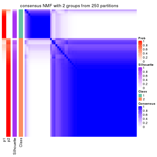
consensus_heatmap(res, k = 3)
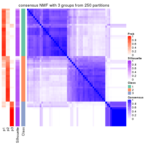
consensus_heatmap(res, k = 4)
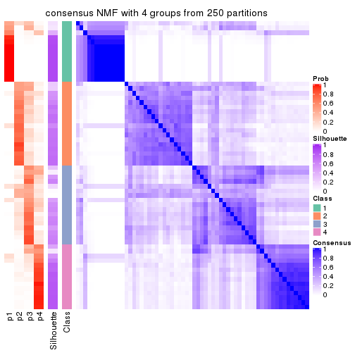
consensus_heatmap(res, k = 5)
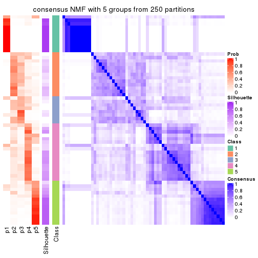
consensus_heatmap(res, k = 6)
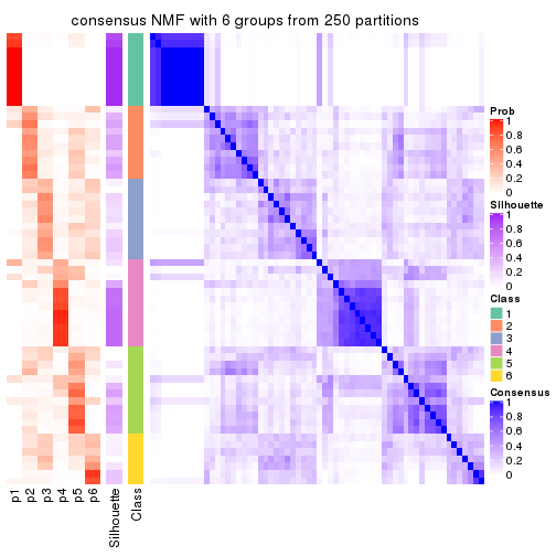
Heatmaps for the membership of samples in all partitions to see how consistent they are:
membership_heatmap(res, k = 2)
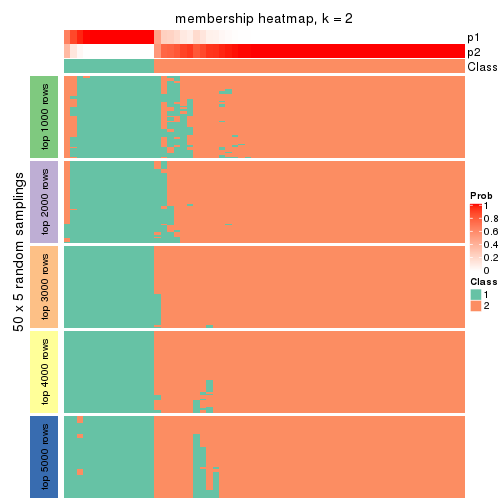
membership_heatmap(res, k = 3)
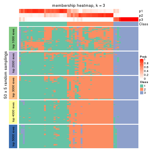
membership_heatmap(res, k = 4)
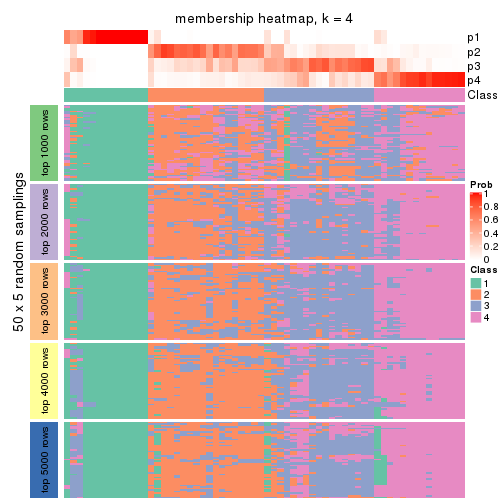
membership_heatmap(res, k = 5)
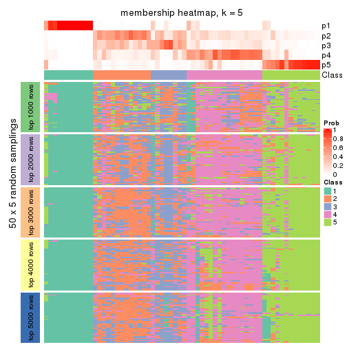
membership_heatmap(res, k = 6)
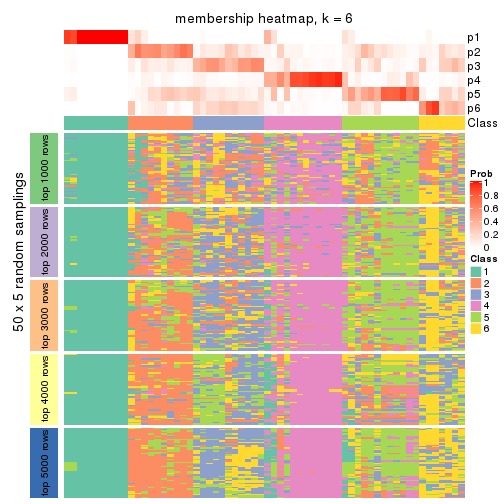
As soon as we have had the classes for columns, we can look for signatures which are significantly different between classes which can be candidate marks for certain classes. Following are the heatmaps for signatures.
Signature heatmaps where rows are scaled:
get_signatures(res, k = 2)
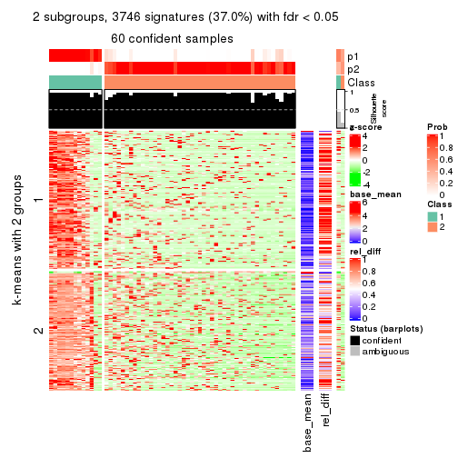
get_signatures(res, k = 3)
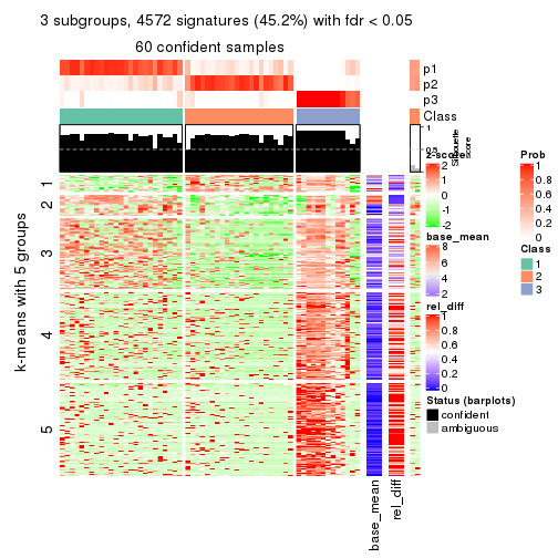
get_signatures(res, k = 4)
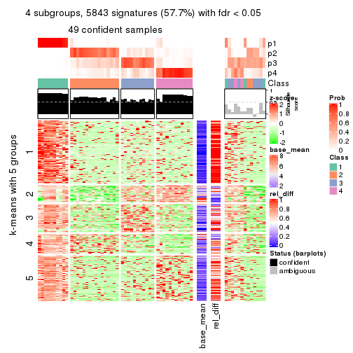
get_signatures(res, k = 5)
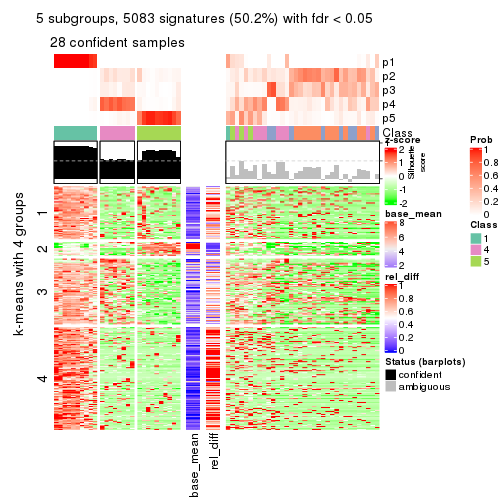
get_signatures(res, k = 6)
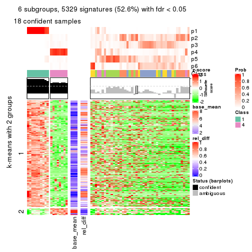
Signature heatmaps where rows are not scaled:
get_signatures(res, k = 2, scale_rows = FALSE)
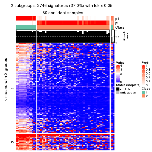
get_signatures(res, k = 3, scale_rows = FALSE)
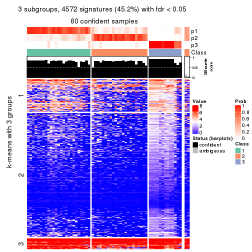
get_signatures(res, k = 4, scale_rows = FALSE)
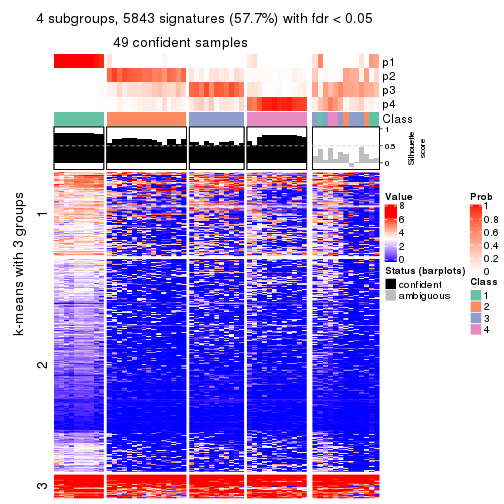
get_signatures(res, k = 5, scale_rows = FALSE)
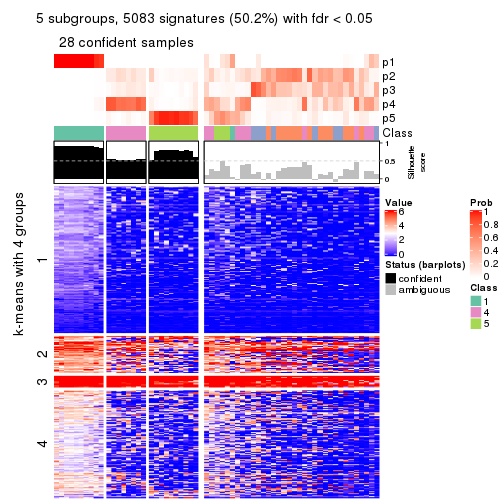
get_signatures(res, k = 6, scale_rows = FALSE)
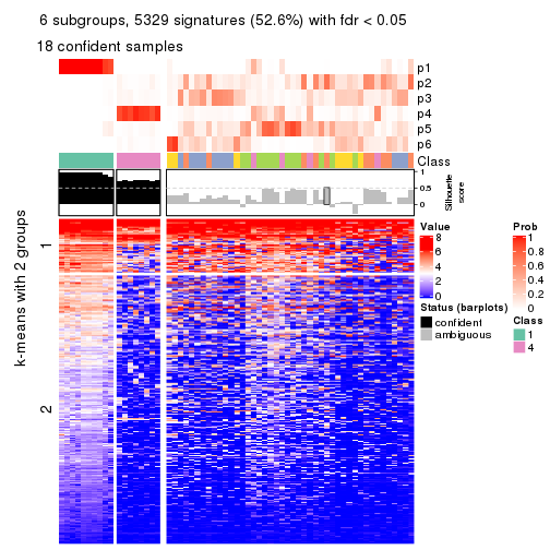
Compare the overlap of signatures from different k:
compare_signatures(res)
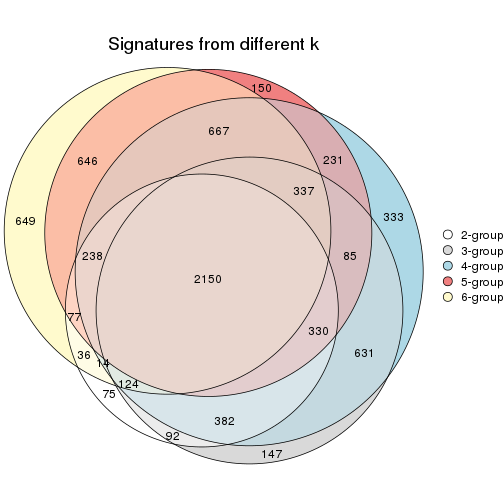
get_signature() returns a data frame invisibly. TO get the list of signatures, the function
call should be assigned to a variable explicitly. In following code, if plot argument is set
to FALSE, no heatmap is plotted while only the differential analysis is performed.
# code only for demonstration
tb = get_signature(res, k = ..., plot = FALSE)
An example of the output of tb is:
#> which_row fdr mean_1 mean_2 scaled_mean_1 scaled_mean_2 km
#> 1 38 0.042760348 8.373488 9.131774 -0.5533452 0.5164555 1
#> 2 40 0.018707592 7.106213 8.469186 -0.6173731 0.5762149 1
#> 3 55 0.019134737 10.221463 11.207825 -0.6159697 0.5749050 1
#> 4 59 0.006059896 5.921854 7.869574 -0.6899429 0.6439467 1
#> 5 60 0.018055526 8.928898 10.211722 -0.6204761 0.5791110 1
#> 6 98 0.009384629 15.714769 14.887706 0.6635654 -0.6193277 2
...
The columns in tb are:
which_row: row indices corresponding to the input matrix.fdr: FDR for the differential test. mean_x: The mean value in group x.scaled_mean_x: The mean value in group x after rows are scaled.km: Row groups if k-means clustering is applied to rows.UMAP plot which shows how samples are separated.
dimension_reduction(res, k = 2, method = "UMAP")
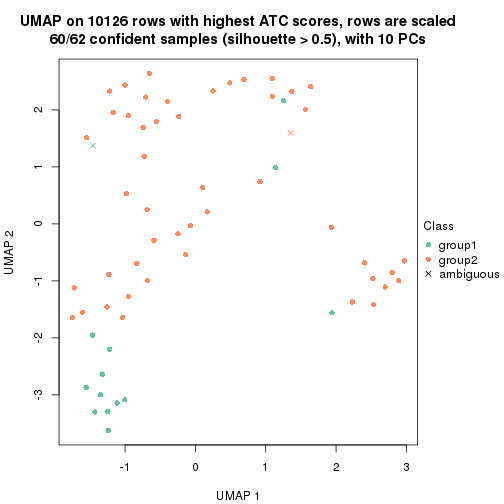
dimension_reduction(res, k = 3, method = "UMAP")
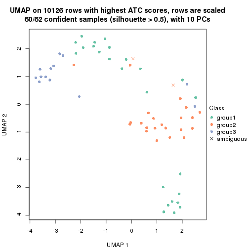
dimension_reduction(res, k = 4, method = "UMAP")
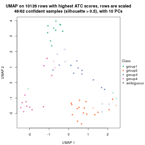
dimension_reduction(res, k = 5, method = "UMAP")
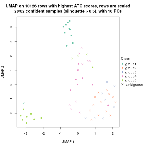
dimension_reduction(res, k = 6, method = "UMAP")
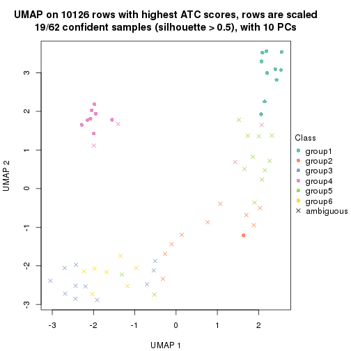
Following heatmap shows how subgroups are split when increasing k:
collect_classes(res)
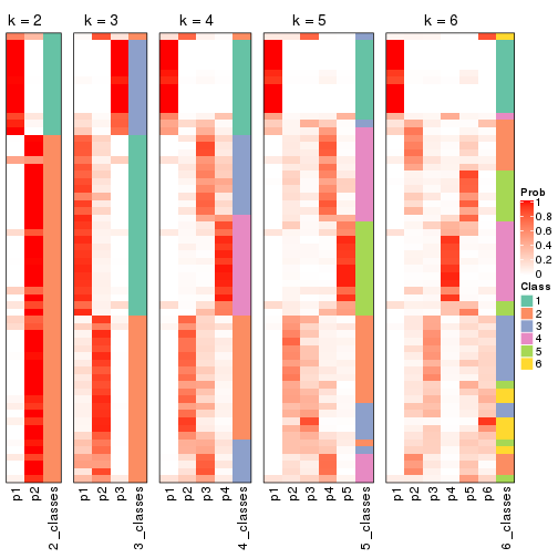
If matrix rows can be associated to genes, consider to use functional_enrichment(res,
...) to perform function enrichment for the signature genes. See this vignette for more detailed explanations.
sessionInfo()
#> R version 3.6.0 (2019-04-26)
#> Platform: x86_64-pc-linux-gnu (64-bit)
#> Running under: CentOS Linux 7 (Core)
#>
#> Matrix products: default
#> BLAS: /usr/lib64/libblas.so.3.4.2
#> LAPACK: /usr/lib64/liblapack.so.3.4.2
#>
#> locale:
#> [1] LC_CTYPE=en_GB.UTF-8 LC_NUMERIC=C LC_TIME=en_GB.UTF-8
#> [4] LC_COLLATE=en_GB.UTF-8 LC_MONETARY=en_GB.UTF-8 LC_MESSAGES=en_GB.UTF-8
#> [7] LC_PAPER=en_GB.UTF-8 LC_NAME=C LC_ADDRESS=C
#> [10] LC_TELEPHONE=C LC_MEASUREMENT=en_GB.UTF-8 LC_IDENTIFICATION=C
#>
#> attached base packages:
#> [1] grid stats graphics grDevices utils datasets methods base
#>
#> other attached packages:
#> [1] genefilter_1.66.0 ComplexHeatmap_2.3.1 markdown_1.1 knitr_1.26
#> [5] GetoptLong_0.1.7 cola_1.3.2
#>
#> loaded via a namespace (and not attached):
#> [1] circlize_0.4.8 shape_1.4.4 xfun_0.11 slam_0.1-46
#> [5] lattice_0.20-38 splines_3.6.0 colorspace_1.4-1 vctrs_0.2.0
#> [9] stats4_3.6.0 blob_1.2.0 XML_3.98-1.20 survival_2.44-1.1
#> [13] rlang_0.4.2 pillar_1.4.2 DBI_1.0.0 BiocGenerics_0.30.0
#> [17] bit64_0.9-7 RColorBrewer_1.1-2 matrixStats_0.55.0 stringr_1.4.0
#> [21] GlobalOptions_0.1.1 evaluate_0.14 memoise_1.1.0 Biobase_2.44.0
#> [25] IRanges_2.18.3 parallel_3.6.0 AnnotationDbi_1.46.1 highr_0.8
#> [29] Rcpp_1.0.3 xtable_1.8-4 backports_1.1.5 S4Vectors_0.22.1
#> [33] annotate_1.62.0 skmeans_0.2-11 bit_1.1-14 microbenchmark_1.4-7
#> [37] brew_1.0-6 impute_1.58.0 rjson_0.2.20 png_0.1-7
#> [41] digest_0.6.23 stringi_1.4.3 polyclip_1.10-0 clue_0.3-57
#> [45] tools_3.6.0 bitops_1.0-6 magrittr_1.5 eulerr_6.0.0
#> [49] RCurl_1.95-4.12 RSQLite_2.1.4 tibble_2.1.3 cluster_2.1.0
#> [53] crayon_1.3.4 pkgconfig_2.0.3 zeallot_0.1.0 Matrix_1.2-17
#> [57] xml2_1.2.2 httr_1.4.1 R6_2.4.1 mclust_5.4.5
#> [61] compiler_3.6.0