
Date: 2019-12-25 23:35:42 CET, cola version: 1.3.2
Document is loading...
All available functions which can be applied to this res_list object:
res_list
#> A 'ConsensusPartitionList' object with 24 methods.
#>   On a matrix with 626 rows and 70 columns.
#>   Top rows are extracted by 'SD, CV, MAD, ATC' methods.
#>   Subgroups are detected by 'hclust, kmeans, skmeans, pam, mclust, NMF' method.
#>   Number of partitions are tried for k = 2, 3, 4, 5, 6.
#>   Performed in total 30000 partitions by row resampling.
#>
#> Following methods can be applied to this 'ConsensusPartitionList' object:
#>  [1] "cola_report"           "collect_classes"       "collect_plots"         "collect_stats"
#>  [5] "colnames"              "functional_enrichment" "get_anno_col"          "get_anno"
#>  [9] "get_classes"           "get_matrix"            "get_membership"        "get_stats"
#> [13] "is_best_k"             "is_stable_k"           "ncol"                  "nrow"
#> [17] "rownames"              "show"                  "suggest_best_k"        "test_to_known_factors"
#> [21] "top_rows_heatmap"      "top_rows_overlap"
#>
#> You can get result for a single method by, e.g. object["SD", "hclust"] or object["SD:hclust"]
#> or a subset of methods by object[c("SD", "CV")], c("hclust", "kmeans")]
The call of run_all_consensus_partition_methods() was:
#> run_all_consensus_partition_methods(data = mat, mc.cores = 4)
Dimension of the input matrix:
mat = get_matrix(res_list)
dim(mat)
#> [1] 626 70
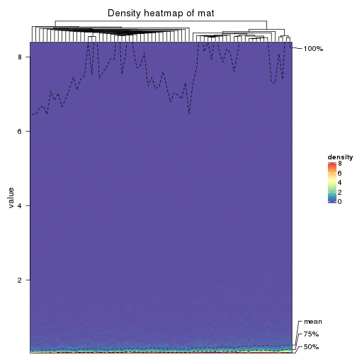
The density distribution for each sample is visualized as in one column in the following heatmap. The clustering is based on the distance which is the Kolmogorov-Smirnov statistic between two distributions.
library(ComplexHeatmap)
densityHeatmap(mat, ylab = "value", cluster_columns = TRUE, show_column_names = FALSE,
    mc.cores = 4)
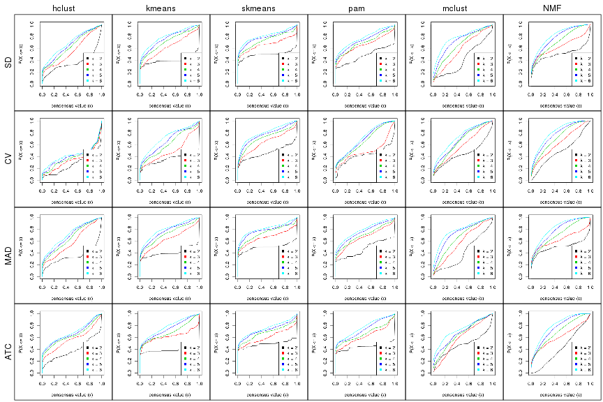
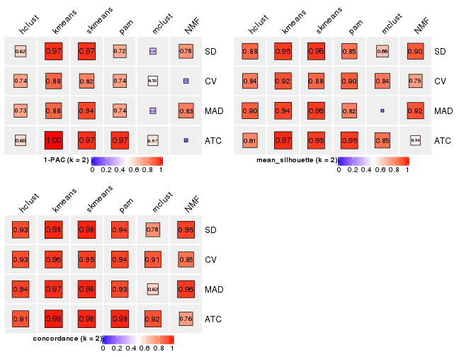
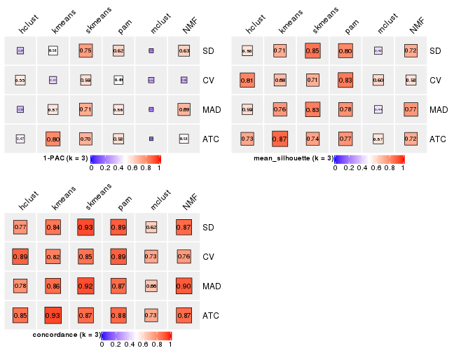
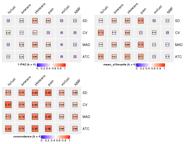
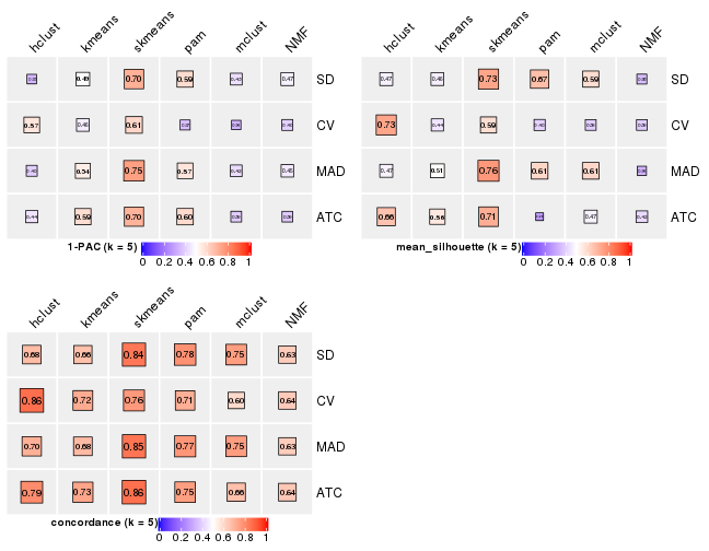
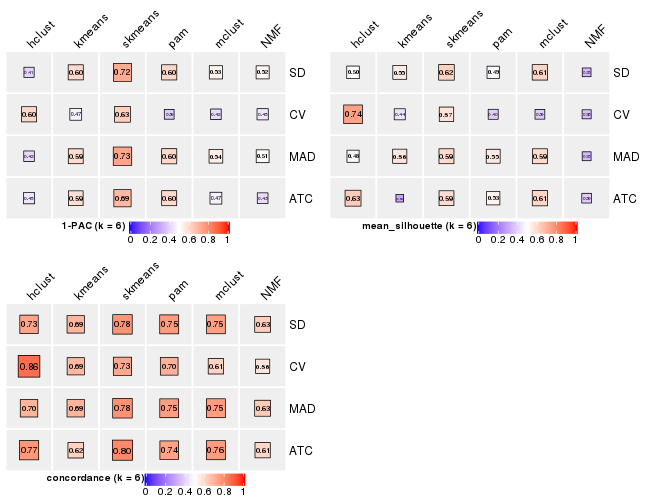
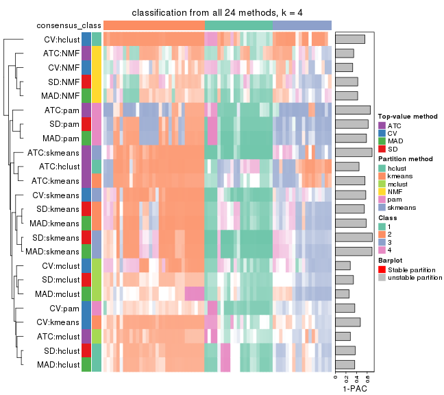
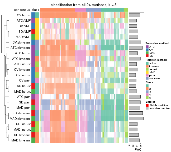
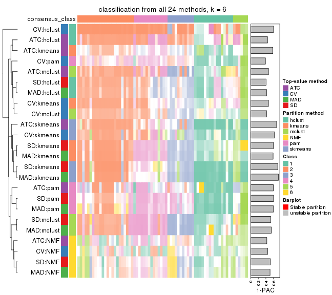
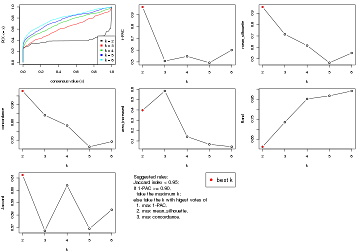
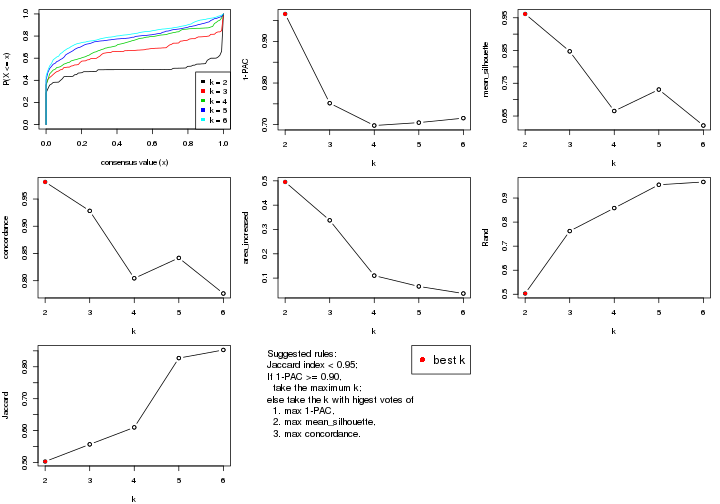
Folowing table shows the best k (number of partitions) for each combination
of top-value methods and partition methods. Clicking on the method name in
the table goes to the section for a single combination of methods.
The cola vignette explains the definition of the metrics used for determining the best number of partitions.
suggest_best_k(res_list)
| The best k | 1-PAC | Mean silhouette | Concordance | ||
|---|---|---|---|---|---|
| ATC:kmeans | 2 | 1.000 | 0.974 | 0.988 | ** |
| ATC:skmeans | 2 | 0.969 | 0.954 | 0.980 | ** |
| ATC:pam | 2 | 0.969 | 0.954 | 0.980 | ** |
| SD:kmeans | 2 | 0.966 | 0.954 | 0.978 | ** |
| SD:skmeans | 2 | 0.966 | 0.962 | 0.981 | ** |
| MAD:skmeans | 2 | 0.939 | 0.956 | 0.979 | * |
| MAD:NMF | 2 | 0.831 | 0.917 | 0.957 | |
| CV:skmeans | 2 | 0.819 | 0.880 | 0.949 | |
| SD:NMF | 2 | 0.779 | 0.901 | 0.949 | |
| MAD:pam | 2 | 0.744 | 0.823 | 0.930 | |
| CV:pam | 2 | 0.742 | 0.899 | 0.944 | |
| SD:pam | 2 | 0.718 | 0.855 | 0.939 | |
| ATC:mclust | 2 | 0.572 | 0.850 | 0.916 | |
| MAD:kmeans | 3 | 0.567 | 0.764 | 0.864 | |
| CV:hclust | 3 | 0.554 | 0.812 | 0.887 | |
| CV:mclust | 2 | 0.533 | 0.841 | 0.908 | |
| ATC:NMF | 3 | 0.512 | 0.716 | 0.866 | |
| ATC:hclust | 3 | 0.469 | 0.728 | 0.853 | |
| MAD:mclust | 5 | 0.423 | 0.606 | 0.752 | |
| CV:kmeans | 3 | 0.405 | 0.676 | 0.820 | |
| SD:hclust | 3 | 0.369 | 0.576 | 0.772 | |
| MAD:hclust | 3 | 0.354 | 0.591 | 0.775 | |
| SD:mclust | 2 | 0.350 | 0.661 | 0.781 | |
| CV:NMF | 2 | 0.258 | 0.749 | 0.853 |
**: 1-PAC > 0.95, *: 1-PAC > 0.9
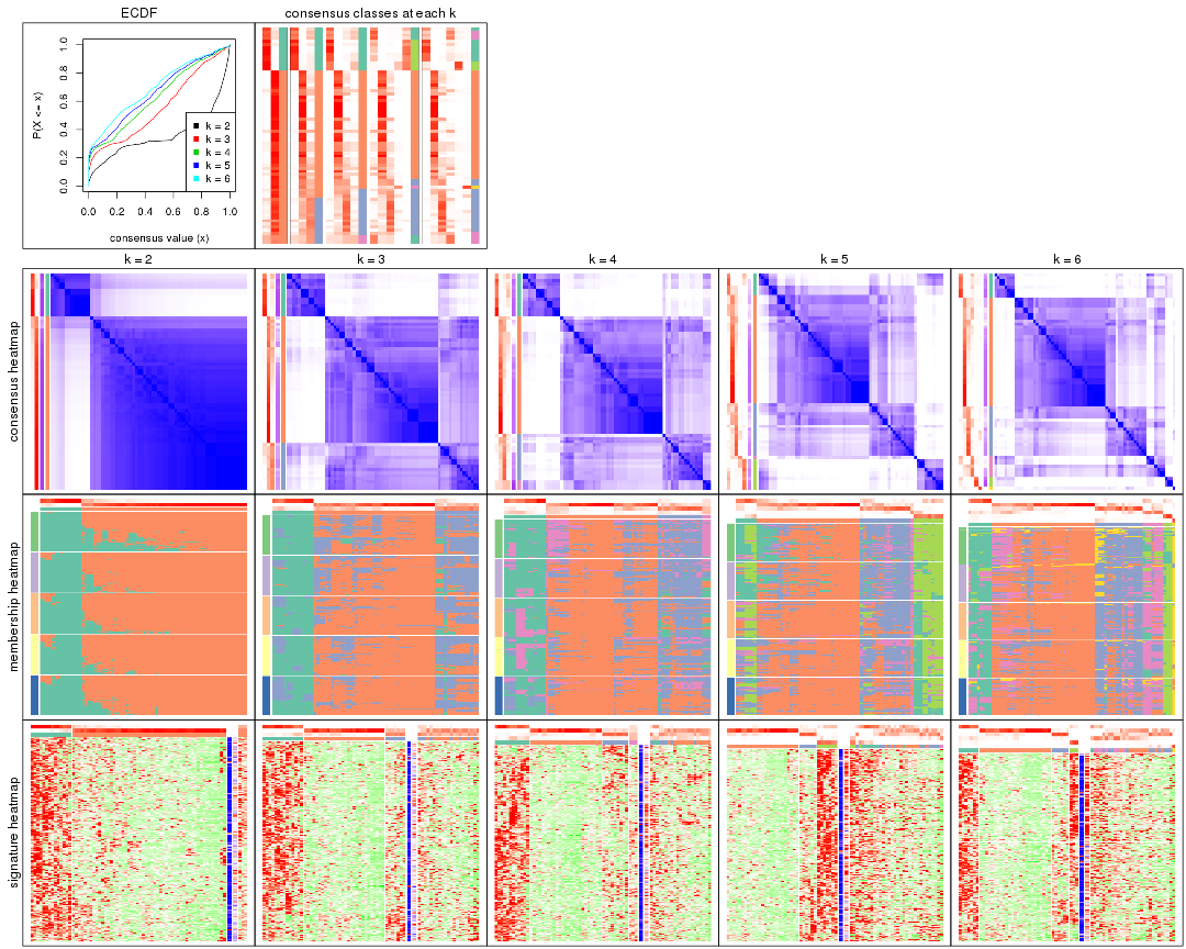
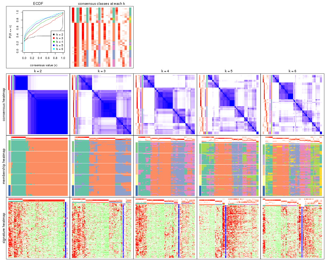
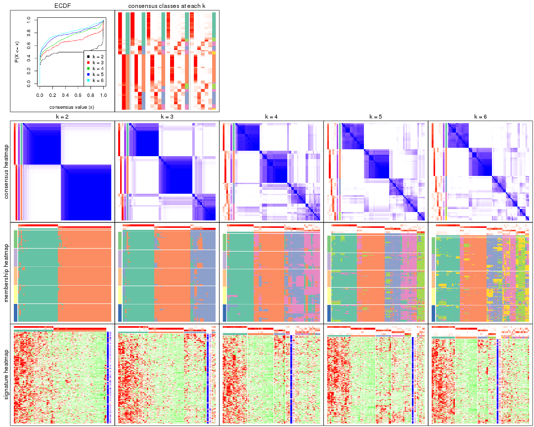
Cumulative distribution function curves of consensus matrix for all methods.
collect_plots(res_list, fun = plot_ecdf)
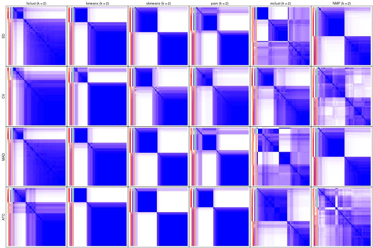
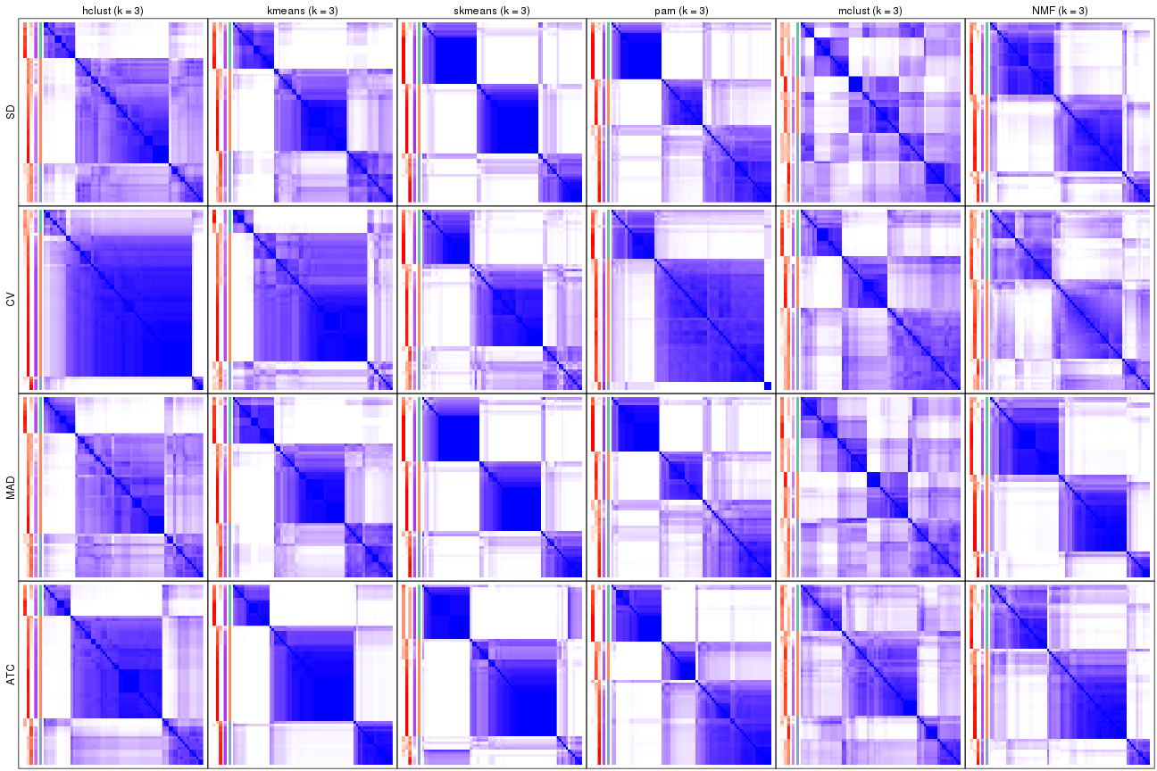
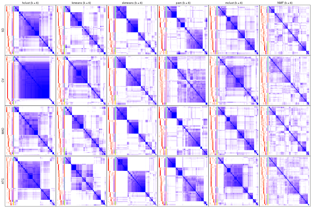
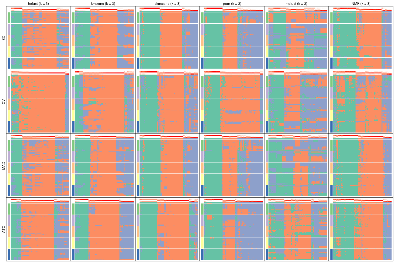
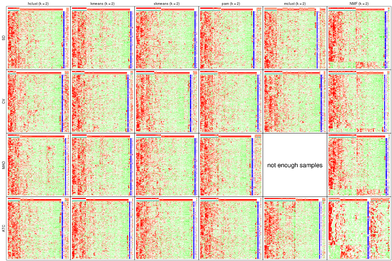
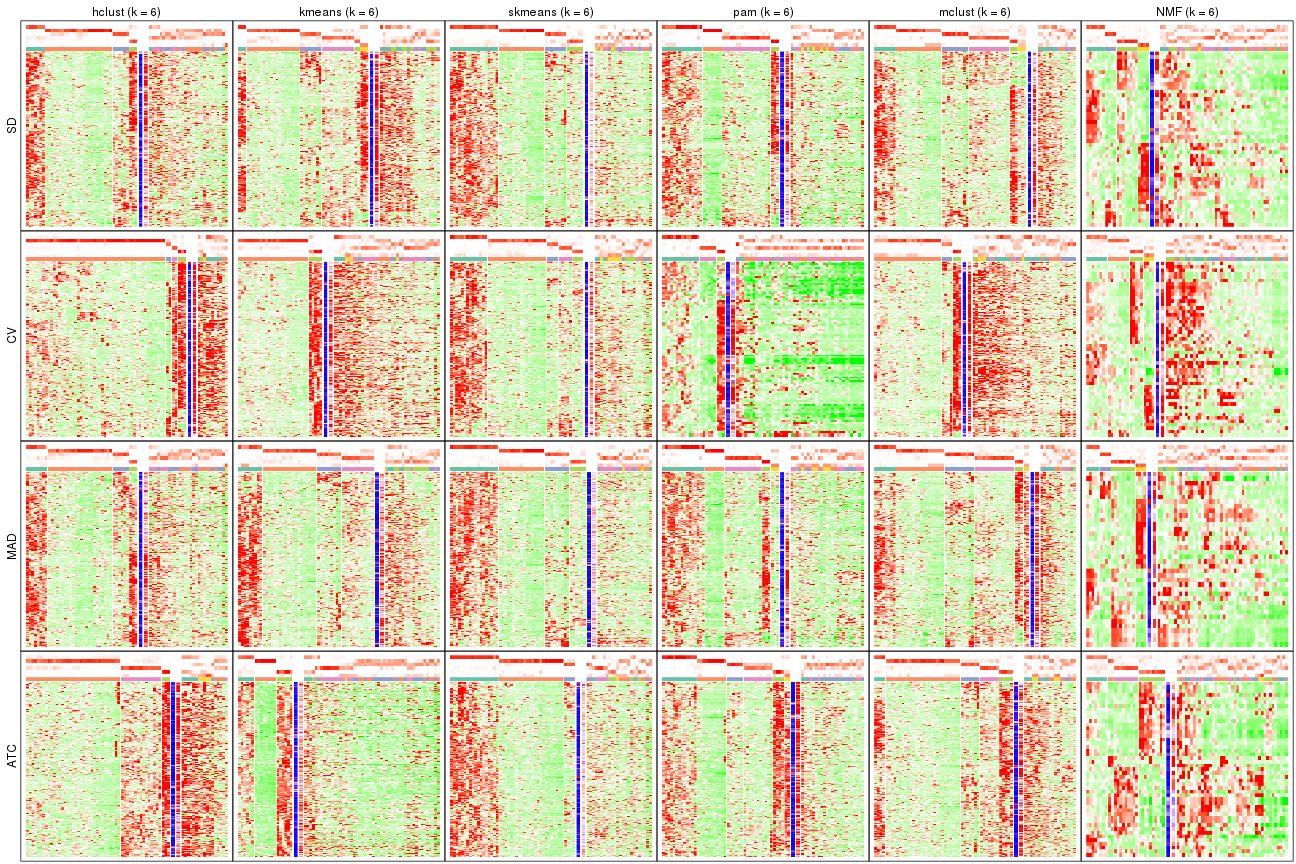
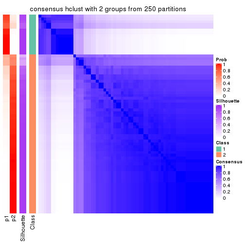
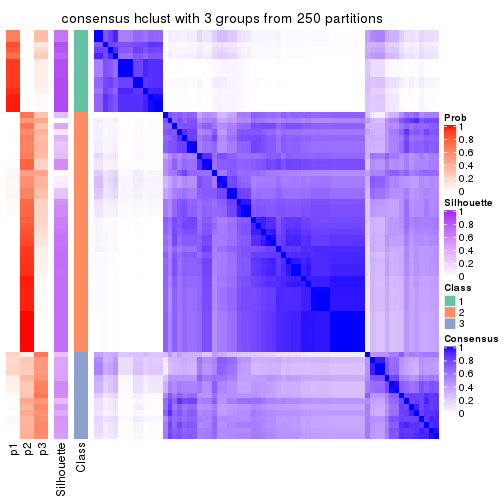
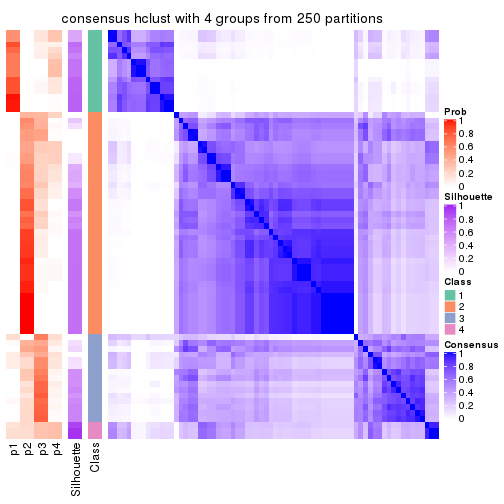
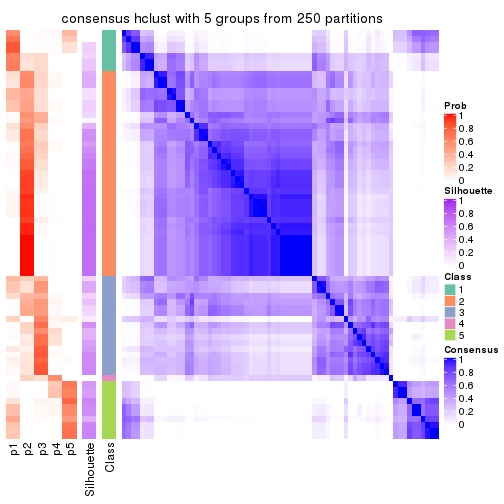
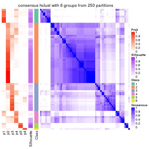
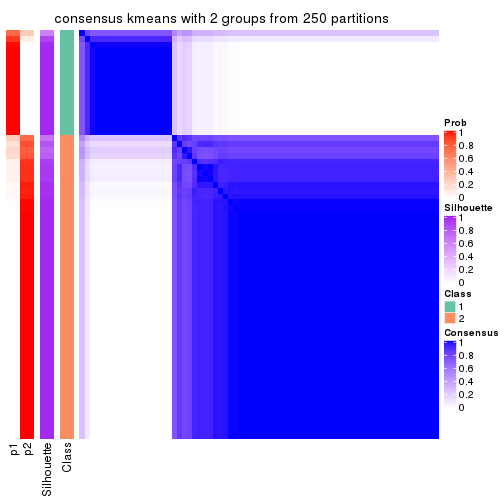
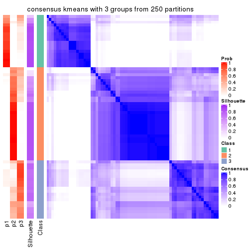
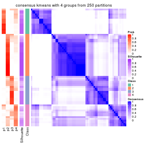
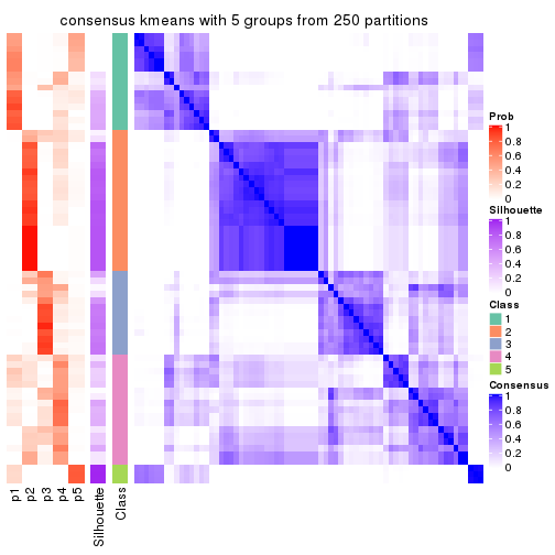
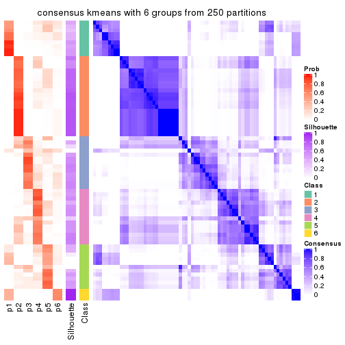
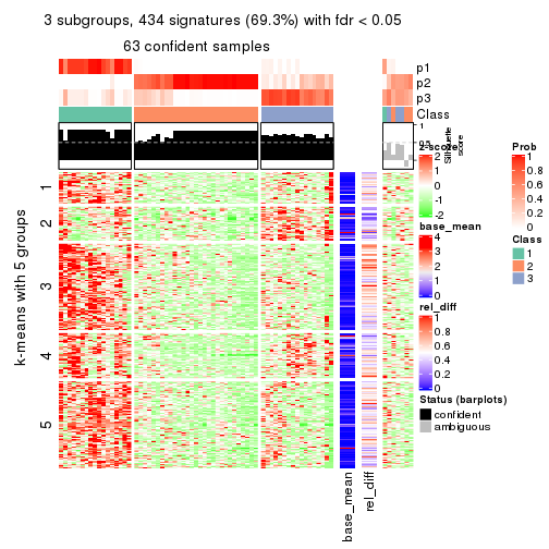
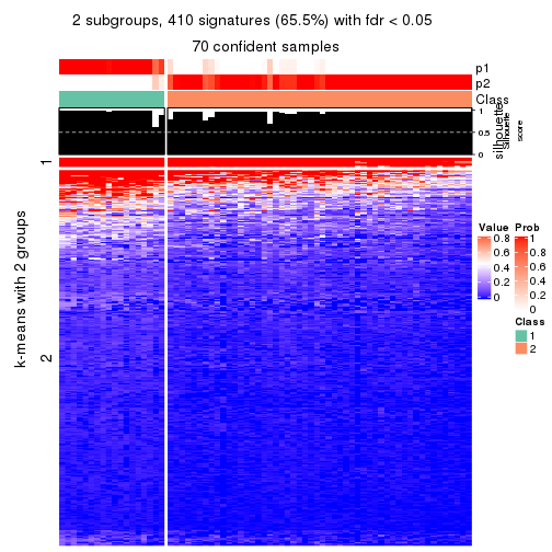
Consensus heatmaps for all methods. (What is a consensus heatmap?)
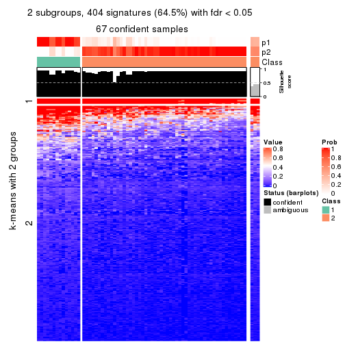
collect_plots(res_list, k = 2, fun = consensus_heatmap, mc.cores = 4)
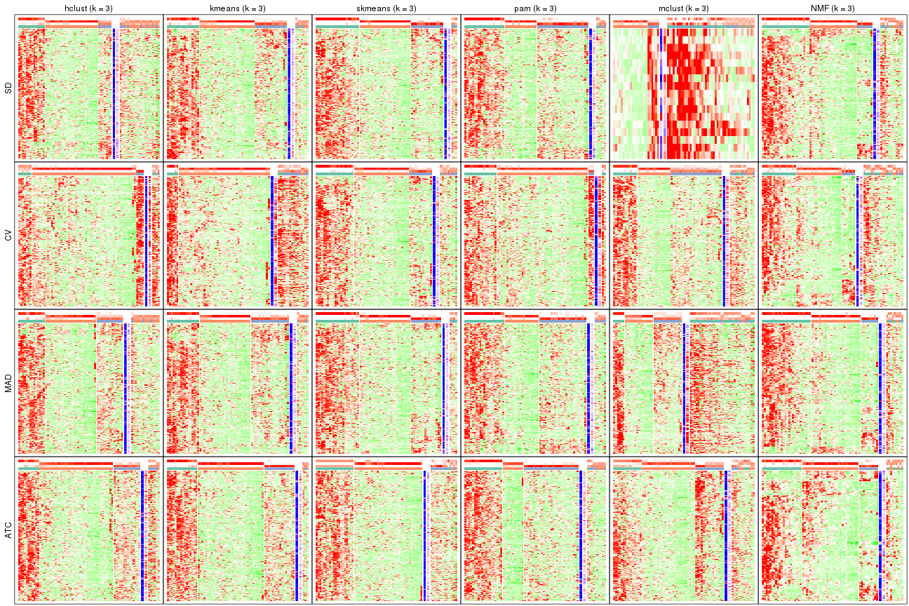
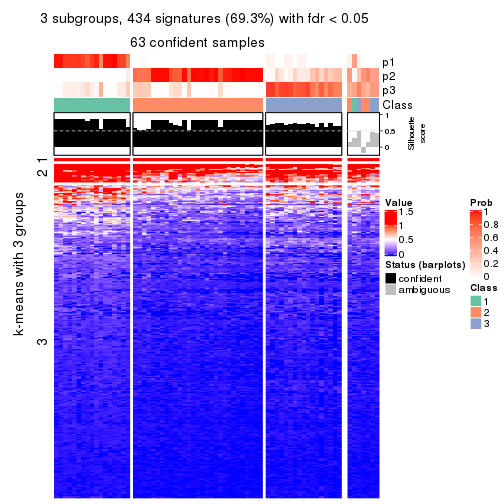
collect_plots(res_list, k = 3, fun = consensus_heatmap, mc.cores = 4)
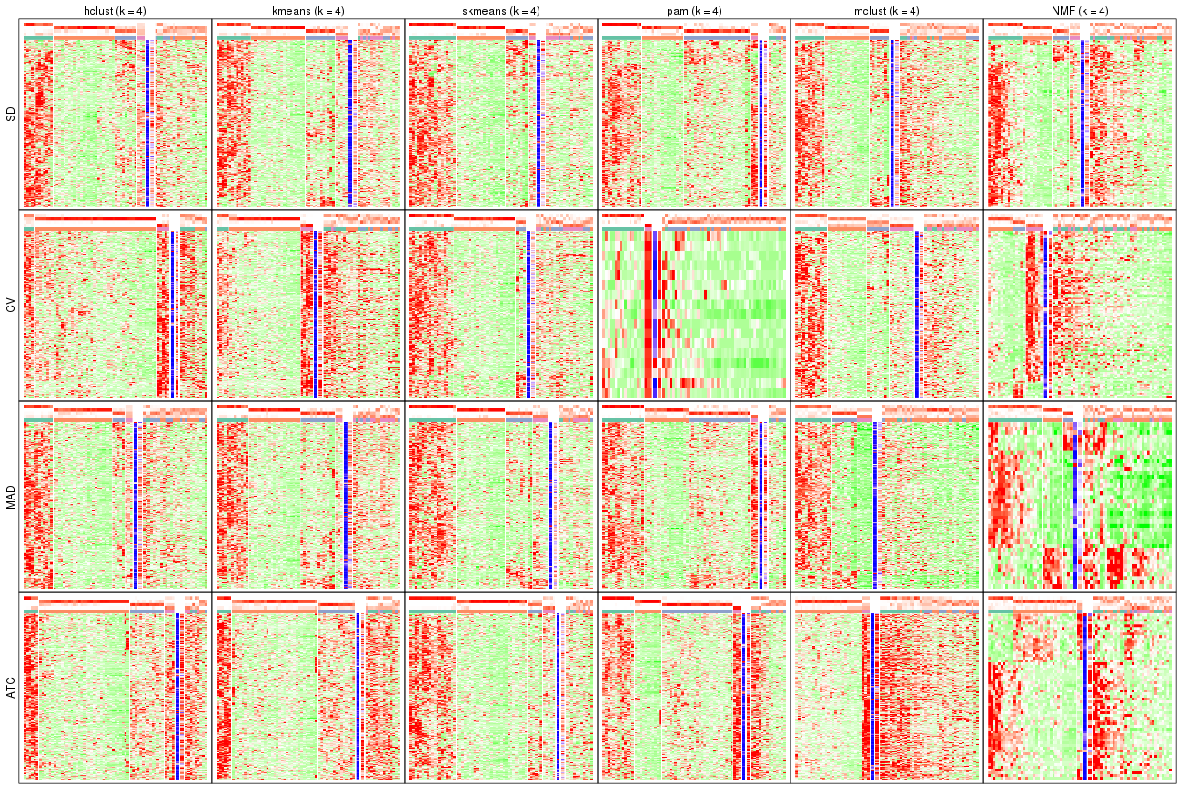
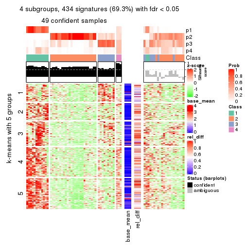
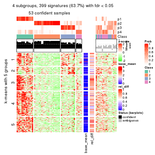
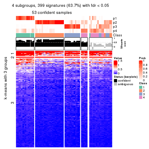
collect_plots(res_list, k = 4, fun = consensus_heatmap, mc.cores = 4)
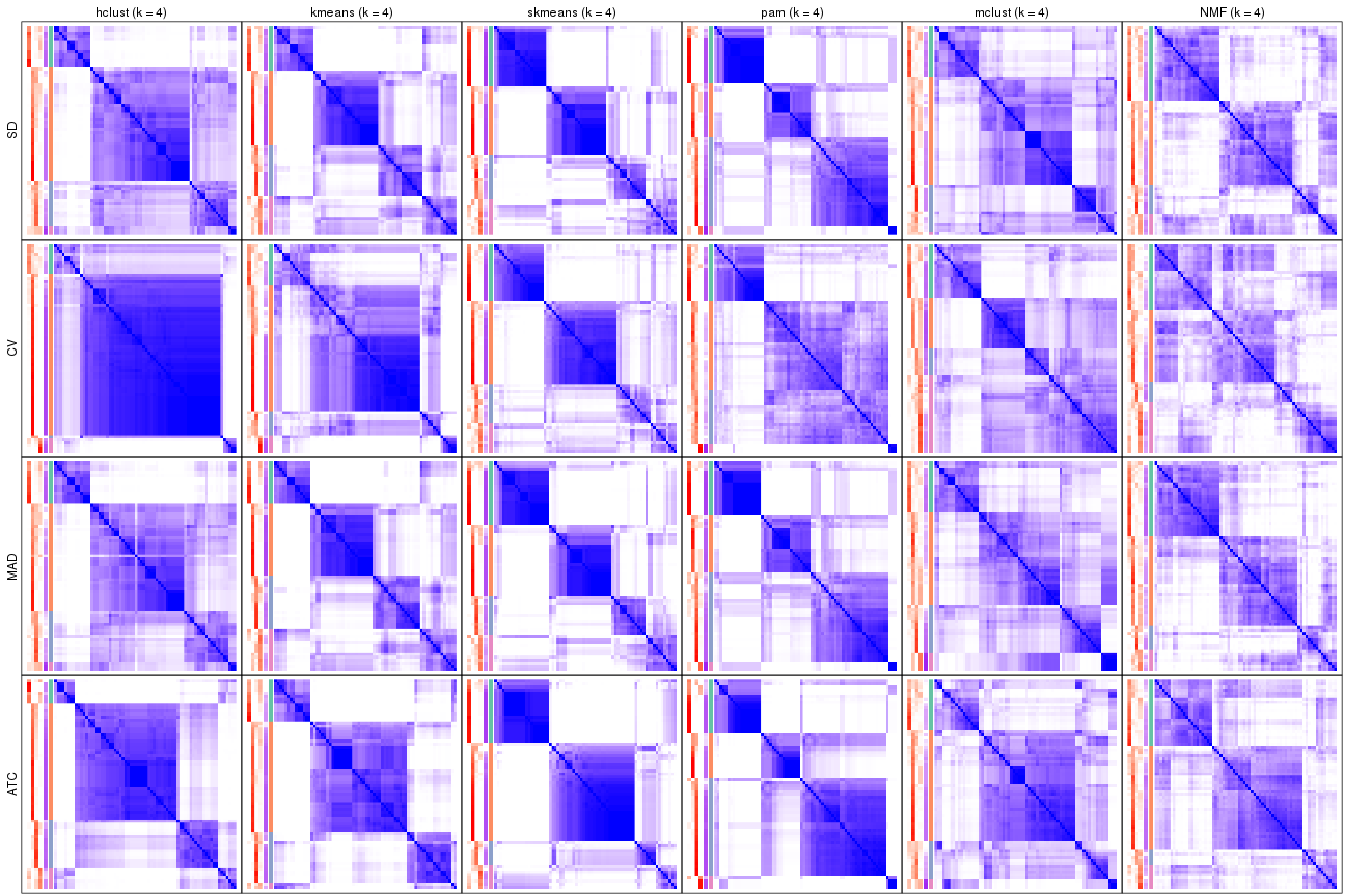
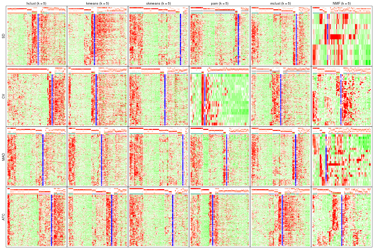
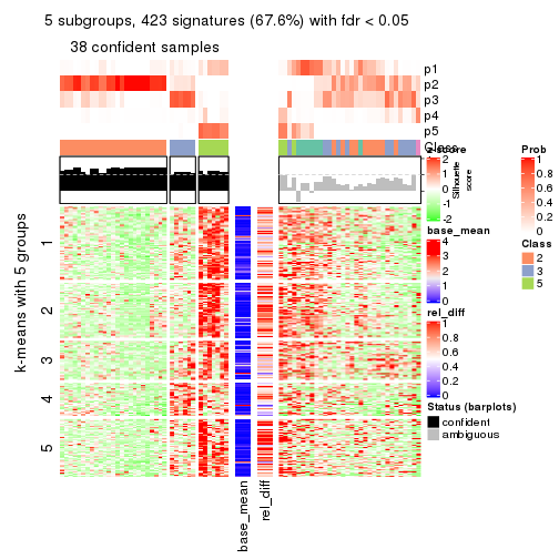
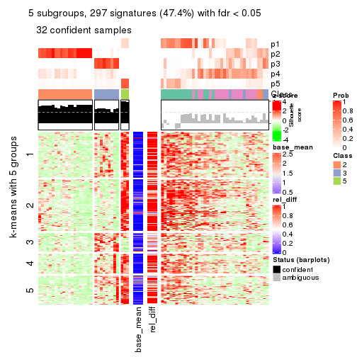
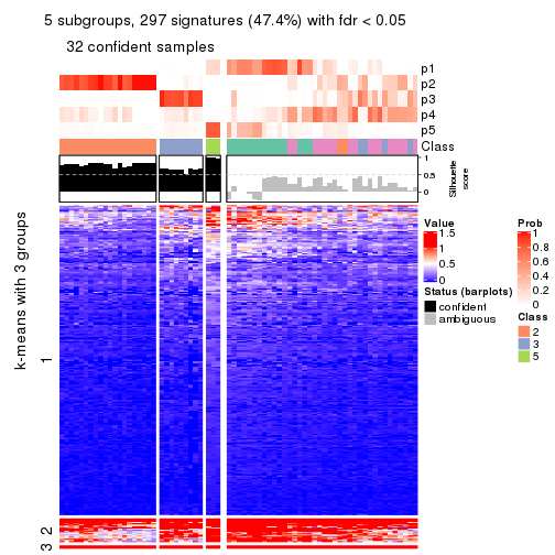
collect_plots(res_list, k = 5, fun = consensus_heatmap, mc.cores = 4)
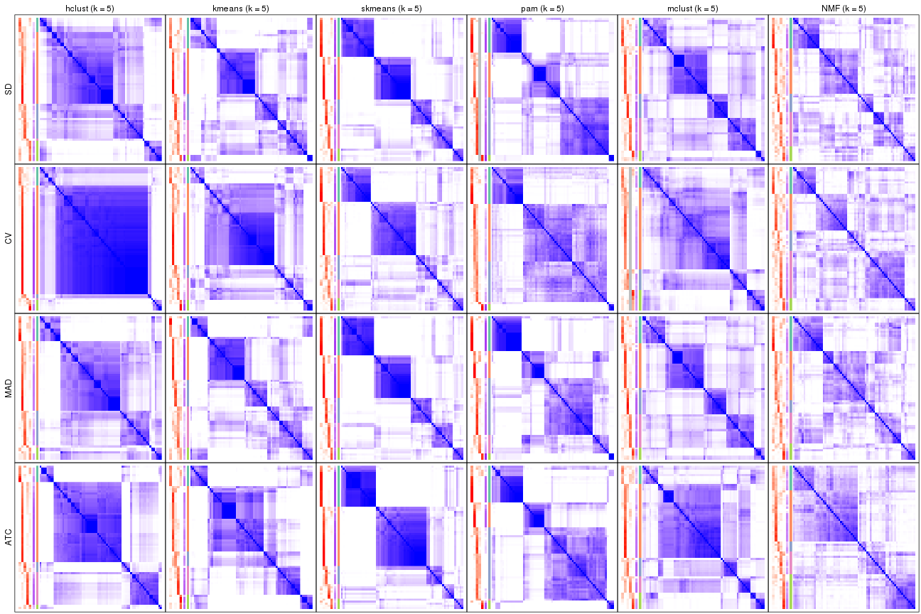
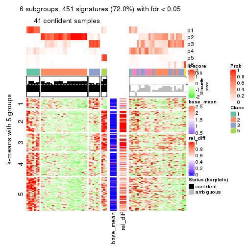
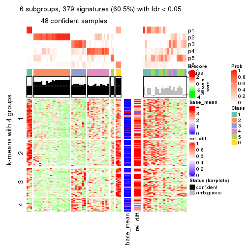
collect_plots(res_list, k = 6, fun = consensus_heatmap, mc.cores = 4)
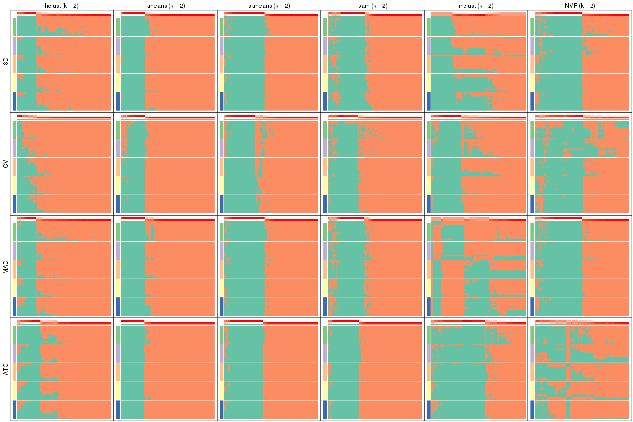
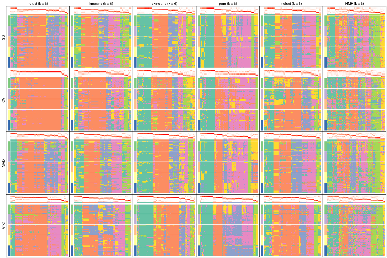
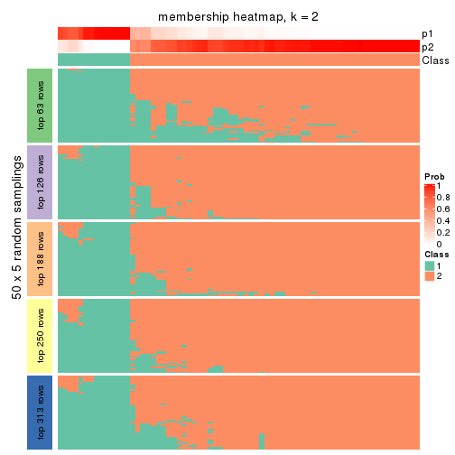
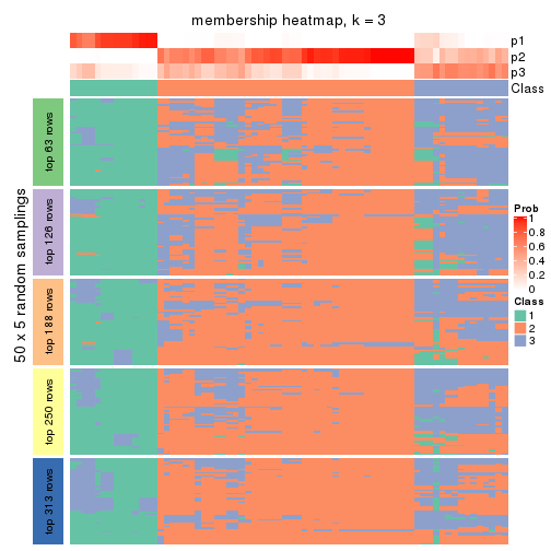
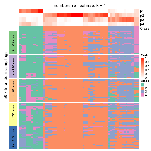
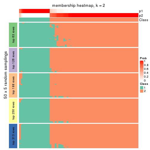
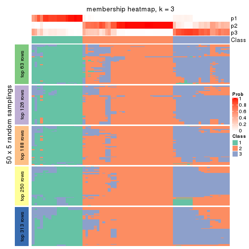
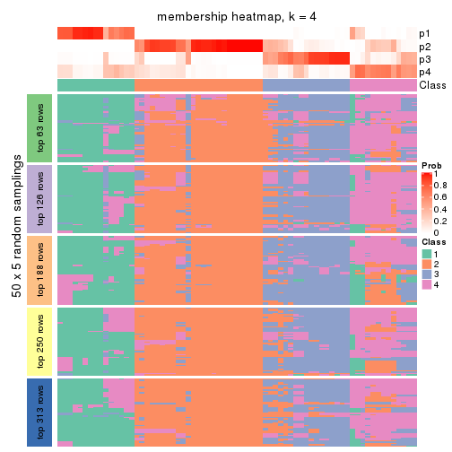
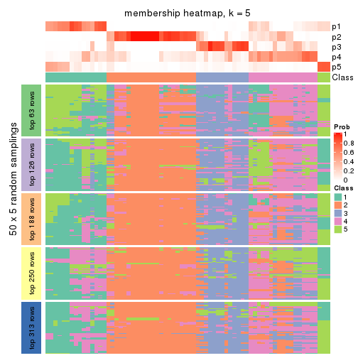
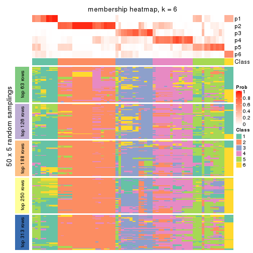
Membership heatmaps for all methods. (What is a membership heatmap?)
collect_plots(res_list, k = 2, fun = membership_heatmap, mc.cores = 4)
collect_plots(res_list, k = 3, fun = membership_heatmap, mc.cores = 4)
collect_plots(res_list, k = 4, fun = membership_heatmap, mc.cores = 4)
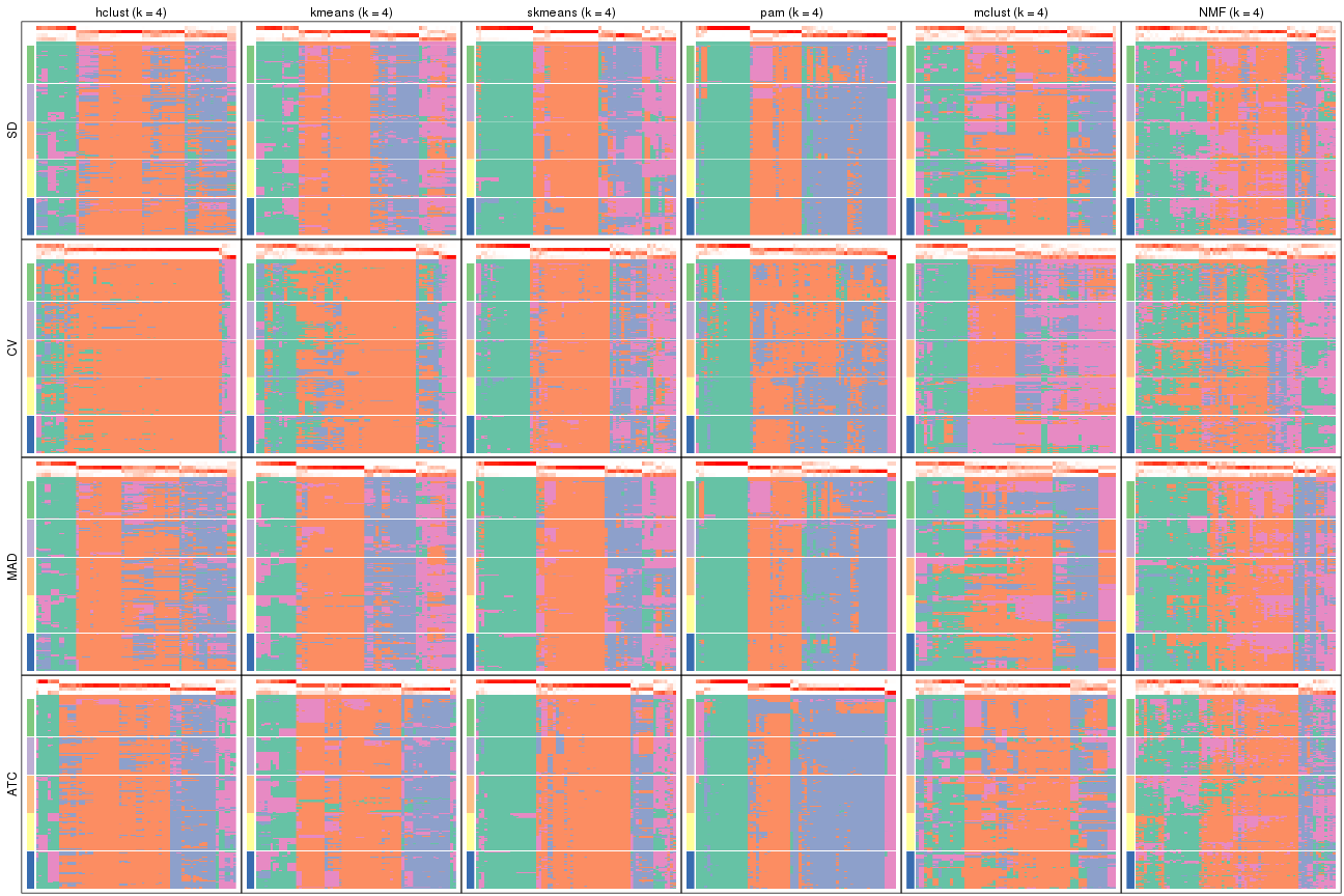
collect_plots(res_list, k = 5, fun = membership_heatmap, mc.cores = 4)
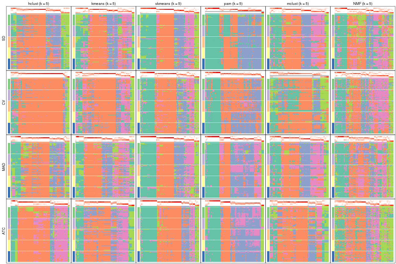
collect_plots(res_list, k = 6, fun = membership_heatmap, mc.cores = 4)
Signature heatmaps for all methods. (What is a signature heatmap?)
Note in following heatmaps, rows are scaled.
collect_plots(res_list, k = 2, fun = get_signatures, mc.cores = 4)
collect_plots(res_list, k = 3, fun = get_signatures, mc.cores = 4)
collect_plots(res_list, k = 4, fun = get_signatures, mc.cores = 4)
collect_plots(res_list, k = 5, fun = get_signatures, mc.cores = 4)
collect_plots(res_list, k = 6, fun = get_signatures, mc.cores = 4)
The statistics used for measuring the stability of consensus partitioning. (How are they defined?)
get_stats(res_list, k = 2)
#>             k 1-PAC mean_silhouette concordance area_increased  Rand Jaccard
#> SD:NMF      2 0.779           0.901       0.949          0.503 0.493   0.493
#> CV:NMF      2 0.258           0.749       0.853          0.493 0.493   0.493
#> MAD:NMF     2 0.831           0.917       0.957          0.504 0.493   0.493
#> ATC:NMF     2 0.196           0.538       0.756          0.420 0.552   0.552
#> SD:skmeans  2 0.966           0.962       0.981          0.495 0.503   0.503
#> CV:skmeans  2 0.819           0.880       0.949          0.467 0.552   0.552
#> MAD:skmeans 2 0.939           0.956       0.979          0.497 0.503   0.503
#> ATC:skmeans 2 0.969           0.954       0.980          0.489 0.508   0.508
#> SD:mclust   2 0.350           0.661       0.781          0.418 0.658   0.658
#> CV:mclust   2 0.533           0.841       0.908          0.448 0.563   0.563
#> MAD:mclust  2 0.319           0.159       0.617          0.411 0.817   0.817
#> ATC:mclust  2 0.572           0.850       0.916          0.473 0.503   0.503
#> SD:kmeans   2 0.966           0.954       0.978          0.397 0.612   0.612
#> CV:kmeans   2 0.881           0.918       0.960          0.359 0.612   0.612
#> MAD:kmeans  2 0.882           0.941       0.972          0.408 0.612   0.612
#> ATC:kmeans  2 1.000           0.974       0.988          0.385 0.627   0.627
#> SD:pam      2 0.718           0.855       0.939          0.475 0.513   0.513
#> CV:pam      2 0.742           0.899       0.944          0.427 0.563   0.563
#> MAD:pam     2 0.744           0.823       0.930          0.469 0.519   0.519
#> ATC:pam     2 0.969           0.954       0.980          0.444 0.552   0.552
#> SD:hclust   2 0.622           0.878       0.928          0.358 0.675   0.675
#> CV:hclust   2 0.742           0.838       0.926          0.260 0.712   0.712
#> MAD:hclust  2 0.728           0.896       0.942          0.342 0.675   0.675
#> ATC:hclust  2 0.597           0.807       0.914          0.386 0.627   0.627
get_stats(res_list, k = 3)
#>             k 1-PAC mean_silhouette concordance area_increased  Rand Jaccard
#> SD:NMF      3 0.626           0.716       0.871          0.263 0.778   0.588
#> CV:NMF      3 0.341           0.579       0.759          0.284 0.708   0.492
#> MAD:NMF     3 0.691           0.770       0.901          0.247 0.806   0.636
#> ATC:NMF     3 0.512           0.716       0.866          0.461 0.699   0.516
#> SD:skmeans  3 0.752           0.847       0.928          0.338 0.763   0.557
#> CV:skmeans  3 0.587           0.707       0.850          0.375 0.771   0.595
#> MAD:skmeans 3 0.715           0.827       0.922          0.337 0.776   0.577
#> ATC:skmeans 3 0.702           0.740       0.868          0.240 0.873   0.755
#> SD:mclust   3 0.237           0.424       0.623          0.401 0.595   0.418
#> CV:mclust   3 0.311           0.605       0.728          0.305 0.692   0.494
#> MAD:mclust  3 0.238           0.440       0.657          0.428 0.436   0.343
#> ATC:mclust  3 0.205           0.570       0.728          0.247 0.740   0.533
#> SD:kmeans   3 0.508           0.715       0.841          0.583 0.735   0.567
#> CV:kmeans   3 0.405           0.676       0.820          0.386 0.918   0.867
#> MAD:kmeans  3 0.567           0.764       0.864          0.560 0.730   0.560
#> ATC:kmeans  3 0.798           0.874       0.935          0.609 0.742   0.592
#> SD:pam      3 0.616           0.803       0.893          0.383 0.707   0.488
#> CV:pam      3 0.493           0.835       0.891          0.162 0.976   0.958
#> MAD:pam     3 0.565           0.783       0.868          0.407 0.669   0.443
#> ATC:pam     3 0.584           0.774       0.877          0.400 0.779   0.609
#> SD:hclust   3 0.369           0.576       0.772          0.567 0.745   0.623
#> CV:hclust   3 0.554           0.812       0.887          0.316 0.933   0.907
#> MAD:hclust  3 0.354           0.591       0.775          0.705 0.725   0.594
#> ATC:hclust  3 0.469           0.728       0.853          0.466 0.733   0.592
get_stats(res_list, k = 4)
#>             k 1-PAC mean_silhouette concordance area_increased  Rand Jaccard
#> SD:NMF      4 0.423           0.434       0.663         0.1320 0.864   0.663
#> CV:NMF      4 0.327           0.328       0.620         0.1321 0.733   0.412
#> MAD:NMF     4 0.421           0.476       0.695         0.1412 0.839   0.627
#> ATC:NMF     4 0.346           0.487       0.678         0.1346 0.911   0.786
#> SD:skmeans  4 0.698           0.665       0.804         0.1103 0.858   0.610
#> CV:skmeans  4 0.574           0.647       0.795         0.1170 0.871   0.658
#> MAD:skmeans 4 0.692           0.688       0.817         0.1116 0.882   0.667
#> ATC:skmeans 4 0.693           0.706       0.855         0.1252 0.897   0.753
#> SD:mclust   4 0.341           0.355       0.696         0.1321 0.751   0.472
#> CV:mclust   4 0.281           0.537       0.653         0.1325 0.865   0.640
#> MAD:mclust  4 0.258           0.441       0.618         0.1348 0.732   0.410
#> ATC:mclust  4 0.283           0.406       0.679         0.1046 0.827   0.611
#> SD:kmeans   4 0.547           0.616       0.783         0.1417 0.851   0.604
#> CV:kmeans   4 0.471           0.489       0.765         0.2414 0.807   0.665
#> MAD:kmeans  4 0.581           0.632       0.791         0.1375 0.843   0.583
#> ATC:kmeans  4 0.559           0.606       0.777         0.1183 0.988   0.970
#> SD:pam      4 0.619           0.745       0.851         0.0609 0.976   0.930
#> CV:pam      4 0.367           0.408       0.726         0.3299 0.776   0.585
#> MAD:pam     4 0.587           0.745       0.848         0.0592 0.978   0.934
#> ATC:pam     4 0.662           0.710       0.861         0.0764 0.970   0.917
#> SD:hclust   4 0.375           0.525       0.717         0.1292 0.923   0.823
#> CV:hclust   4 0.558           0.734       0.870         0.1181 0.951   0.926
#> MAD:hclust  4 0.366           0.519       0.721         0.1280 0.920   0.810
#> ATC:hclust  4 0.447           0.705       0.824         0.1207 0.941   0.861
get_stats(res_list, k = 5)
#>             k 1-PAC mean_silhouette concordance area_increased  Rand Jaccard
#> SD:NMF      5 0.469           0.362       0.633         0.0870 0.791   0.432
#> CV:NMF      5 0.399           0.390       0.637         0.0794 0.845   0.527
#> MAD:NMF     5 0.454           0.335       0.631         0.0867 0.820   0.512
#> ATC:NMF     5 0.388           0.422       0.643         0.0892 0.825   0.544
#> SD:skmeans  5 0.705           0.731       0.842         0.0659 0.955   0.827
#> CV:skmeans  5 0.606           0.585       0.762         0.0695 0.912   0.710
#> MAD:skmeans 5 0.746           0.764       0.846         0.0620 0.949   0.807
#> ATC:skmeans 5 0.697           0.711       0.856         0.0647 0.927   0.783
#> SD:mclust   5 0.429           0.587       0.750         0.1047 0.810   0.512
#> CV:mclust   5 0.340           0.394       0.596         0.0424 0.735   0.419
#> MAD:mclust  5 0.423           0.606       0.752         0.1107 0.813   0.471
#> ATC:mclust  5 0.391           0.472       0.663         0.0457 0.902   0.748
#> SD:kmeans   5 0.493           0.465       0.663         0.0675 0.867   0.569
#> CV:kmeans   5 0.460           0.444       0.718         0.0839 0.923   0.821
#> MAD:kmeans  5 0.545           0.506       0.679         0.0614 0.864   0.555
#> ATC:kmeans  5 0.590           0.559       0.733         0.0814 0.882   0.691
#> SD:pam      5 0.590           0.668       0.780         0.0649 0.931   0.802
#> CV:pam      5 0.366           0.404       0.708         0.0490 0.954   0.862
#> MAD:pam     5 0.568           0.605       0.769         0.0785 0.929   0.781
#> ATC:pam     5 0.597           0.281       0.747         0.1024 0.932   0.815
#> SD:hclust   5 0.348           0.470       0.675         0.0524 0.922   0.800
#> CV:hclust   5 0.569           0.732       0.859         0.0682 0.974   0.958
#> MAD:hclust  5 0.397           0.472       0.703         0.0496 0.957   0.881
#> ATC:hclust  5 0.441           0.658       0.792         0.0481 0.989   0.972
get_stats(res_list, k = 6)
#>             k 1-PAC mean_silhouette concordance area_increased  Rand Jaccard
#> SD:NMF      6 0.518           0.347       0.630         0.0478 0.865   0.492
#> CV:NMF      6 0.447           0.361       0.565         0.0497 0.965   0.848
#> MAD:NMF     6 0.511           0.353       0.634         0.0516 0.845   0.446
#> ATC:NMF     6 0.426           0.386       0.608         0.0576 0.914   0.672
#> SD:skmeans  6 0.716           0.621       0.776         0.0367 0.967   0.853
#> CV:skmeans  6 0.629           0.574       0.726         0.0452 0.972   0.885
#> MAD:skmeans 6 0.732           0.594       0.779         0.0377 0.987   0.940
#> ATC:skmeans 6 0.685           0.592       0.801         0.0425 0.968   0.892
#> SD:mclust   6 0.527           0.613       0.747         0.0672 0.959   0.826
#> CV:mclust   6 0.421           0.389       0.612         0.0636 0.841   0.609
#> MAD:mclust  6 0.545           0.595       0.753         0.0587 0.969   0.863
#> ATC:mclust  6 0.470           0.608       0.757         0.0796 0.915   0.748
#> SD:kmeans   6 0.600           0.551       0.692         0.0441 0.891   0.584
#> CV:kmeans   6 0.470           0.439       0.685         0.0846 0.879   0.693
#> MAD:kmeans  6 0.592           0.563       0.694         0.0454 0.907   0.639
#> ATC:kmeans  6 0.585           0.304       0.621         0.0472 0.852   0.533
#> SD:pam      6 0.604           0.489       0.754         0.0505 0.913   0.721
#> CV:pam      6 0.390           0.398       0.704         0.0304 0.776   0.470
#> MAD:pam     6 0.602           0.555       0.749         0.0456 0.949   0.811
#> ATC:pam     6 0.598           0.532       0.740         0.0465 0.829   0.528
#> SD:hclust   6 0.406           0.499       0.732         0.0494 0.977   0.931
#> CV:hclust   6 0.604           0.743       0.861         0.0541 0.966   0.944
#> MAD:hclust  6 0.420           0.482       0.696         0.0438 0.966   0.898
#> ATC:hclust  6 0.446           0.633       0.767         0.0325 0.986   0.964
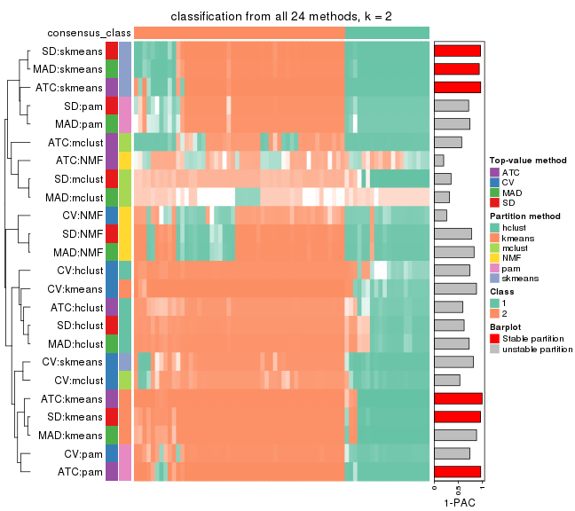
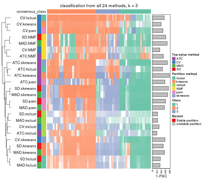
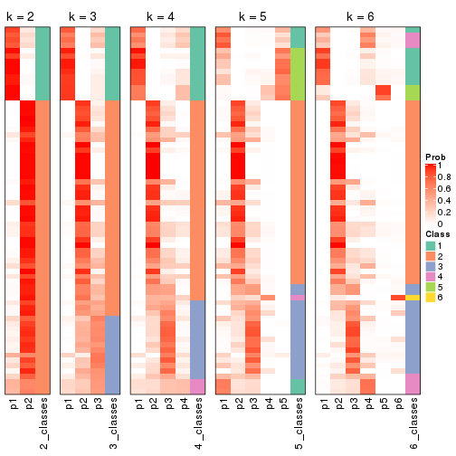
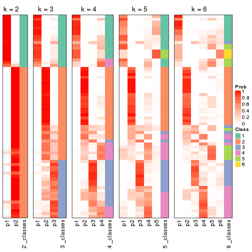
Following heatmap plots the partition for each combination of methods and the lightness correspond to the silhouette scores for samples in each method. On top the consensus subgroup is inferred from all methods by taking the mean silhouette scores as weight.
collect_stats(res_list, k = 2)
collect_stats(res_list, k = 3)
collect_stats(res_list, k = 4)
collect_stats(res_list, k = 5)
collect_stats(res_list, k = 6)
Collect partitions from all methods:
collect_classes(res_list, k = 2)
collect_classes(res_list, k = 3)
collect_classes(res_list, k = 4)
collect_classes(res_list, k = 5)
collect_classes(res_list, k = 6)
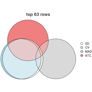
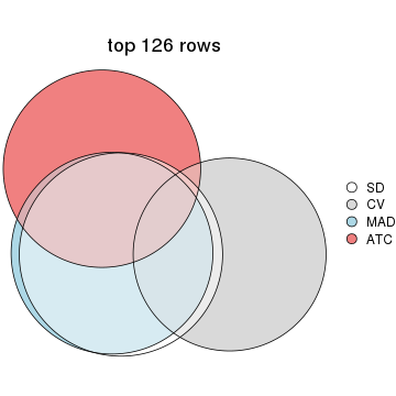
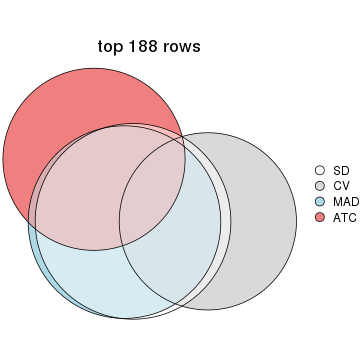
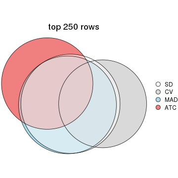
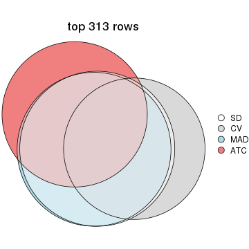
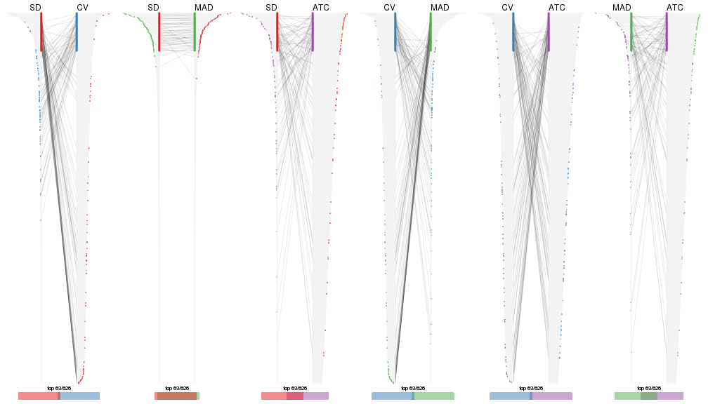
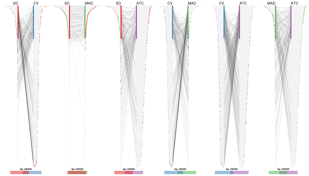
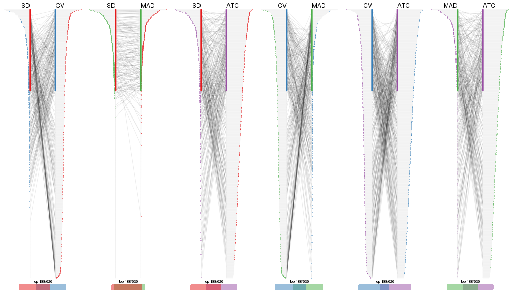
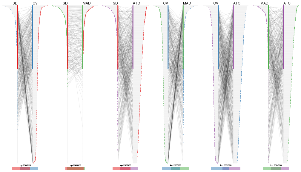
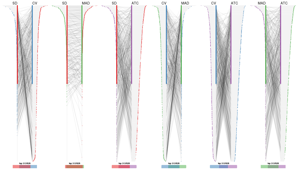
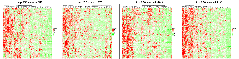
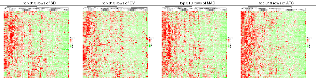
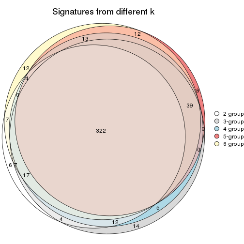
Overlap of top rows from different top-row methods:
top_rows_overlap(res_list, top_n = 63, method = "euler")
top_rows_overlap(res_list, top_n = 126, method = "euler")
top_rows_overlap(res_list, top_n = 188, method = "euler")
top_rows_overlap(res_list, top_n = 250, method = "euler")
top_rows_overlap(res_list, top_n = 313, method = "euler")
Also visualize the correspondance of rankings between different top-row methods:
top_rows_overlap(res_list, top_n = 63, method = "correspondance")
top_rows_overlap(res_list, top_n = 126, method = "correspondance")
top_rows_overlap(res_list, top_n = 188, method = "correspondance")
top_rows_overlap(res_list, top_n = 250, method = "correspondance")
top_rows_overlap(res_list, top_n = 313, method = "correspondance")
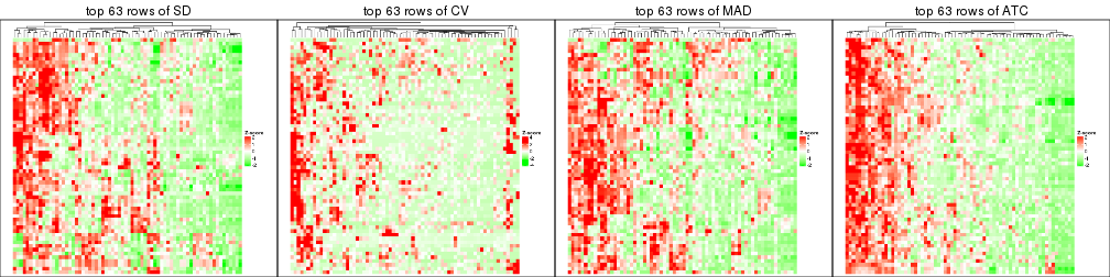
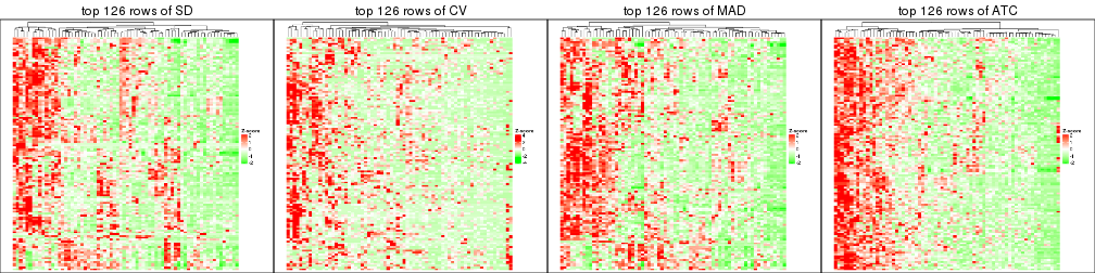
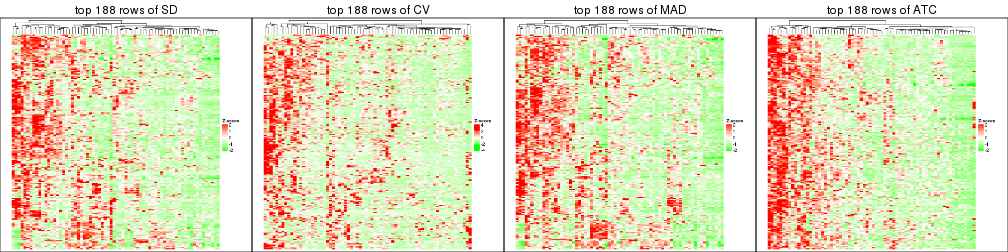
Heatmaps of the top rows:
top_rows_heatmap(res_list, top_n = 63)
top_rows_heatmap(res_list, top_n = 126)
top_rows_heatmap(res_list, top_n = 188)
top_rows_heatmap(res_list, top_n = 250)
top_rows_heatmap(res_list, top_n = 313)
The object with results only for a single top-value method and a single partition method can be extracted as:
res = res_list["SD", "hclust"]
# you can also extract it by
# res = res_list["SD:hclust"]
A summary of res and all the functions that can be applied to it:
res
#> A 'ConsensusPartition' object with k = 2, 3, 4, 5, 6.
#>   On a matrix with 626 rows and 70 columns.
#>   Top rows (63, 126, 188, 250, 313) are extracted by 'SD' method.
#>   Subgroups are detected by 'hclust' method.
#>   Performed in total 1250 partitions by row resampling.
#>   Best k for subgroups seems to be 3.
#>
#> Following methods can be applied to this 'ConsensusPartition' object:
#>  [1] "cola_report"             "collect_classes"         "collect_plots"
#>  [4] "collect_stats"           "colnames"                "compare_signatures"
#>  [7] "consensus_heatmap"       "dimension_reduction"     "functional_enrichment"
#> [10] "get_anno_col"            "get_anno"                "get_classes"
#> [13] "get_consensus"           "get_matrix"              "get_membership"
#> [16] "get_param"               "get_signatures"          "get_stats"
#> [19] "is_best_k"               "is_stable_k"             "membership_heatmap"
#> [22] "ncol"                    "nrow"                    "plot_ecdf"
#> [25] "rownames"                "select_partition_number" "show"
#> [28] "suggest_best_k"          "test_to_known_factors"
collect_plots() function collects all the plots made from res for all k (number of partitions)
into one single page to provide an easy and fast comparison between different k.
collect_plots(res)
The plots are:
k and the heatmap of
predicted classes for each k.k.k.k.All the plots in panels can be made by individual functions and they are plotted later in this section.
select_partition_number() produces several plots showing different
statistics for choosing “optimized” k. There are following statistics:
k;k, the area increased is defined as \(A_k - A_{k-1}\).The detailed explanations of these statistics can be found in the cola vignette.
Generally speaking, lower PAC score, higher mean silhouette score or higher
concordance corresponds to better partition. Rand index and Jaccard index
measure how similar the current partition is compared to partition with k-1.
If they are too similar, we won't accept k is better than k-1.
select_partition_number(res)
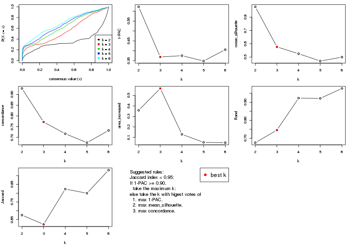
The numeric values for all these statistics can be obtained by get_stats().
get_stats(res)
#>   k 1-PAC mean_silhouette concordance area_increased  Rand Jaccard
#> 2 2 0.622           0.878       0.928         0.3580 0.675   0.675
#> 3 3 0.369           0.576       0.772         0.5665 0.745   0.623
#> 4 4 0.375           0.525       0.717         0.1292 0.923   0.823
#> 5 5 0.348           0.470       0.675         0.0524 0.922   0.800
#> 6 6 0.406           0.499       0.732         0.0494 0.977   0.931
suggest_best_k() suggests the best \(k\) based on these statistics. The rules are as follows:
suggest_best_k(res)
#> [1] 3
Following shows the table of the partitions (You need to click the show/hide
code output link to see it). The membership matrix (columns with name p*)
is inferred by
clue::cl_consensus()
function with the SE method. Basically the value in the membership matrix
represents the probability to belong to a certain group. The finall class
label for an item is determined with the group with highest probability it
belongs to.
In get_classes() function, the entropy is calculated from the membership
matrix and the silhouette score is calculated from the consensus matrix.
cbind(get_classes(res, k = 2), get_membership(res, k = 2))
#>           class entropy silhouette    p1    p2
#> SRR837437     2  0.0376      0.923 0.004 0.996
#> SRR837438     2  0.7376      0.783 0.208 0.792
#> SRR837439     2  0.0376      0.925 0.004 0.996
#> SRR837440     2  0.0672      0.925 0.008 0.992
#> SRR837441     2  0.0000      0.924 0.000 1.000
#> SRR837442     2  0.0376      0.923 0.004 0.996
#> SRR837443     2  0.1414      0.925 0.020 0.980
#> SRR837444     2  0.5294      0.880 0.120 0.880
#> SRR837445     2  0.5408      0.877 0.124 0.876
#> SRR837446     2  0.2423      0.922 0.040 0.960
#> SRR837447     1  0.0672      0.930 0.992 0.008
#> SRR837448     1  0.0376      0.929 0.996 0.004
#> SRR837449     1  0.4690      0.888 0.900 0.100
#> SRR837450     1  0.0376      0.929 0.996 0.004
#> SRR837451     2  0.0376      0.923 0.004 0.996
#> SRR837452     2  0.0672      0.925 0.008 0.992
#> SRR837453     2  0.0376      0.923 0.004 0.996
#> SRR837454     2  0.0376      0.923 0.004 0.996
#> SRR837455     1  0.0376      0.929 0.996 0.004
#> SRR837456     1  0.0376      0.929 0.996 0.004
#> SRR837457     2  0.0376      0.923 0.004 0.996
#> SRR837458     1  0.0376      0.929 0.996 0.004
#> SRR837459     2  0.0376      0.923 0.004 0.996
#> SRR837460     2  0.0376      0.923 0.004 0.996
#> SRR837461     2  0.1633      0.925 0.024 0.976
#> SRR837462     2  0.4939      0.891 0.108 0.892
#> SRR837463     2  0.3584      0.913 0.068 0.932
#> SRR837464     2  0.2948      0.918 0.052 0.948
#> SRR837465     2  0.7602      0.754 0.220 0.780
#> SRR837466     1  0.0376      0.929 0.996 0.004
#> SRR837467     2  0.0376      0.923 0.004 0.996
#> SRR837468     2  0.4431      0.902 0.092 0.908
#> SRR837469     1  0.1633      0.928 0.976 0.024
#> SRR837470     1  0.1633      0.928 0.976 0.024
#> SRR837471     2  0.0672      0.923 0.008 0.992
#> SRR837472     2  0.0672      0.923 0.008 0.992
#> SRR837473     2  0.6712      0.828 0.176 0.824
#> SRR837474     2  0.0672      0.923 0.008 0.992
#> SRR837475     2  0.0672      0.923 0.008 0.992
#> SRR837476     2  0.0376      0.925 0.004 0.996
#> SRR837477     2  0.4161      0.904 0.084 0.916
#> SRR837478     2  0.3431      0.914 0.064 0.936
#> SRR837479     2  0.2423      0.922 0.040 0.960
#> SRR837480     2  0.3431      0.914 0.064 0.936
#> SRR837481     2  0.2948      0.919 0.052 0.948
#> SRR837482     2  0.3431      0.915 0.064 0.936
#> SRR837483     2  0.9754      0.382 0.408 0.592
#> SRR837484     2  0.2043      0.924 0.032 0.968
#> SRR837485     2  0.2043      0.924 0.032 0.968
#> SRR837486     2  0.5294      0.882 0.120 0.880
#> SRR837487     2  0.0376      0.925 0.004 0.996
#> SRR837488     2  0.0376      0.923 0.004 0.996
#> SRR837489     2  0.1414      0.926 0.020 0.980
#> SRR837490     2  0.1414      0.925 0.020 0.980
#> SRR837491     2  0.3584      0.906 0.068 0.932
#> SRR837492     2  0.6531      0.837 0.168 0.832
#> SRR837493     2  0.7376      0.784 0.208 0.792
#> SRR837494     2  0.0376      0.923 0.004 0.996
#> SRR837495     2  0.5519      0.875 0.128 0.872
#> SRR837496     1  0.7139      0.784 0.804 0.196
#> SRR837497     1  0.6148      0.842 0.848 0.152
#> SRR837498     1  0.5178      0.877 0.884 0.116
#> SRR837499     2  0.9661      0.457 0.392 0.608
#> SRR837500     2  0.9661      0.457 0.392 0.608
#> SRR837501     2  0.2603      0.921 0.044 0.956
#> SRR837502     2  0.9460      0.523 0.364 0.636
#> SRR837503     1  0.7139      0.784 0.804 0.196
#> SRR837504     2  0.1184      0.925 0.016 0.984
#> SRR837505     2  0.1633      0.925 0.024 0.976
#> SRR837506     2  0.1184      0.925 0.016 0.984
cbind(get_classes(res, k = 3), get_membership(res, k = 3))
#>           class entropy silhouette    p1    p2    p3
#> SRR837437     2  0.2356     0.7092 0.000 0.928 0.072
#> SRR837438     3  0.7637     0.5867 0.076 0.284 0.640
#> SRR837439     2  0.3686     0.6850 0.000 0.860 0.140
#> SRR837440     2  0.4121     0.6652 0.000 0.832 0.168
#> SRR837441     2  0.3551     0.6862 0.000 0.868 0.132
#> SRR837442     2  0.1163     0.7143 0.000 0.972 0.028
#> SRR837443     2  0.4555     0.6422 0.000 0.800 0.200
#> SRR837444     2  0.7491    -0.1872 0.036 0.492 0.472
#> SRR837445     2  0.7214     0.3107 0.044 0.632 0.324
#> SRR837446     2  0.6057     0.3835 0.004 0.656 0.340
#> SRR837447     1  0.1163     0.8748 0.972 0.000 0.028
#> SRR837448     1  0.2711     0.8502 0.912 0.000 0.088
#> SRR837449     1  0.4345     0.8425 0.848 0.016 0.136
#> SRR837450     1  0.2711     0.8502 0.912 0.000 0.088
#> SRR837451     2  0.0237     0.7081 0.000 0.996 0.004
#> SRR837452     2  0.2711     0.6983 0.000 0.912 0.088
#> SRR837453     2  0.0237     0.7081 0.000 0.996 0.004
#> SRR837454     2  0.0237     0.7081 0.000 0.996 0.004
#> SRR837455     1  0.1031     0.8748 0.976 0.000 0.024
#> SRR837456     1  0.1031     0.8748 0.976 0.000 0.024
#> SRR837457     2  0.0237     0.7081 0.000 0.996 0.004
#> SRR837458     1  0.1964     0.8674 0.944 0.000 0.056
#> SRR837459     2  0.0237     0.7081 0.000 0.996 0.004
#> SRR837460     2  0.0237     0.7081 0.000 0.996 0.004
#> SRR837461     2  0.5621     0.4493 0.000 0.692 0.308
#> SRR837462     3  0.7311     0.5455 0.036 0.384 0.580
#> SRR837463     3  0.6345     0.5141 0.004 0.400 0.596
#> SRR837464     3  0.6168     0.4849 0.000 0.412 0.588
#> SRR837465     3  0.8361     0.4735 0.092 0.364 0.544
#> SRR837466     1  0.2711     0.8502 0.912 0.000 0.088
#> SRR837467     2  0.2165     0.7095 0.000 0.936 0.064
#> SRR837468     3  0.6600     0.5072 0.012 0.384 0.604
#> SRR837469     1  0.2878     0.8675 0.904 0.000 0.096
#> SRR837470     1  0.2878     0.8675 0.904 0.000 0.096
#> SRR837471     2  0.1289     0.7114 0.000 0.968 0.032
#> SRR837472     2  0.1289     0.7114 0.000 0.968 0.032
#> SRR837473     2  0.7519     0.0783 0.044 0.568 0.388
#> SRR837474     2  0.1289     0.7114 0.000 0.968 0.032
#> SRR837475     2  0.1411     0.7096 0.000 0.964 0.036
#> SRR837476     2  0.1031     0.7153 0.000 0.976 0.024
#> SRR837477     2  0.6099     0.5485 0.032 0.740 0.228
#> SRR837478     2  0.5595     0.5782 0.016 0.756 0.228
#> SRR837479     2  0.6386     0.1274 0.004 0.584 0.412
#> SRR837480     2  0.5595     0.5782 0.016 0.756 0.228
#> SRR837481     3  0.6495     0.3291 0.004 0.460 0.536
#> SRR837482     3  0.6451     0.5134 0.008 0.384 0.608
#> SRR837483     3  0.7383     0.3105 0.236 0.084 0.680
#> SRR837484     2  0.5988     0.3077 0.000 0.632 0.368
#> SRR837485     2  0.6008     0.2923 0.000 0.628 0.372
#> SRR837486     3  0.6224     0.5829 0.016 0.296 0.688
#> SRR837487     2  0.2537     0.7100 0.000 0.920 0.080
#> SRR837488     2  0.0237     0.7081 0.000 0.996 0.004
#> SRR837489     2  0.5115     0.5677 0.004 0.768 0.228
#> SRR837490     2  0.4931     0.5709 0.000 0.768 0.232
#> SRR837491     2  0.6033     0.3409 0.004 0.660 0.336
#> SRR837492     2  0.7339     0.1043 0.036 0.572 0.392
#> SRR837493     3  0.7683     0.5891 0.080 0.280 0.640
#> SRR837494     2  0.2066     0.7102 0.000 0.940 0.060
#> SRR837495     2  0.7238     0.2976 0.044 0.628 0.328
#> SRR837496     1  0.6252     0.6865 0.648 0.008 0.344
#> SRR837497     1  0.5517     0.7628 0.728 0.004 0.268
#> SRR837498     1  0.4555     0.8166 0.800 0.000 0.200
#> SRR837499     3  0.9276     0.4586 0.212 0.264 0.524
#> SRR837500     3  0.9276     0.4586 0.212 0.264 0.524
#> SRR837501     3  0.6244     0.4286 0.000 0.440 0.560
#> SRR837502     3  0.9304     0.4494 0.192 0.300 0.508
#> SRR837503     1  0.6252     0.6865 0.648 0.008 0.344
#> SRR837504     2  0.4702     0.6237 0.000 0.788 0.212
#> SRR837505     2  0.6286    -0.2120 0.000 0.536 0.464
#> SRR837506     2  0.5621     0.3301 0.000 0.692 0.308
cbind(get_classes(res, k = 4), get_membership(res, k = 4))
#>           class entropy silhouette    p1    p2    p3    p4
#> SRR837437     2  0.2401    0.69806 0.000 0.904 0.092 0.004
#> SRR837438     3  0.8051    0.14558 0.088 0.192 0.584 0.136
#> SRR837439     2  0.3448    0.66834 0.000 0.828 0.168 0.004
#> SRR837440     2  0.4253    0.62792 0.000 0.776 0.208 0.016
#> SRR837441     2  0.3498    0.66643 0.000 0.832 0.160 0.008
#> SRR837442     2  0.1022    0.70741 0.000 0.968 0.032 0.000
#> SRR837443     2  0.4678    0.59810 0.000 0.744 0.232 0.024
#> SRR837444     3  0.7830    0.15501 0.032 0.400 0.452 0.116
#> SRR837445     2  0.7806    0.12655 0.012 0.508 0.236 0.244
#> SRR837446     2  0.5847    0.16298 0.000 0.560 0.404 0.036
#> SRR837447     1  0.0524    0.77696 0.988 0.000 0.004 0.008
#> SRR837448     1  0.4624    0.69544 0.660 0.000 0.000 0.340
#> SRR837449     1  0.3877    0.73058 0.852 0.004 0.072 0.072
#> SRR837450     1  0.4624    0.69544 0.660 0.000 0.000 0.340
#> SRR837451     2  0.0000    0.70335 0.000 1.000 0.000 0.000
#> SRR837452     2  0.2915    0.69419 0.000 0.892 0.080 0.028
#> SRR837453     2  0.0000    0.70335 0.000 1.000 0.000 0.000
#> SRR837454     2  0.0000    0.70335 0.000 1.000 0.000 0.000
#> SRR837455     1  0.0779    0.77776 0.980 0.000 0.004 0.016
#> SRR837456     1  0.0779    0.77776 0.980 0.000 0.004 0.016
#> SRR837457     2  0.0000    0.70335 0.000 1.000 0.000 0.000
#> SRR837458     1  0.3606    0.75683 0.840 0.000 0.020 0.140
#> SRR837459     2  0.0000    0.70335 0.000 1.000 0.000 0.000
#> SRR837460     2  0.0000    0.70335 0.000 1.000 0.000 0.000
#> SRR837461     2  0.5138    0.28859 0.000 0.600 0.392 0.008
#> SRR837462     3  0.5600    0.58829 0.036 0.188 0.740 0.036
#> SRR837463     3  0.4627    0.61530 0.004 0.196 0.772 0.028
#> SRR837464     3  0.4175    0.62034 0.000 0.200 0.784 0.016
#> SRR837465     3  0.8961   -0.33424 0.096 0.296 0.444 0.164
#> SRR837466     1  0.4564    0.70035 0.672 0.000 0.000 0.328
#> SRR837467     2  0.2149    0.69775 0.000 0.912 0.088 0.000
#> SRR837468     3  0.5354    0.55405 0.004 0.152 0.752 0.092
#> SRR837469     1  0.3931    0.76631 0.832 0.000 0.040 0.128
#> SRR837470     1  0.3931    0.76631 0.832 0.000 0.040 0.128
#> SRR837471     2  0.2124    0.70419 0.000 0.932 0.028 0.040
#> SRR837472     2  0.2124    0.70419 0.000 0.932 0.028 0.040
#> SRR837473     2  0.7904   -0.13781 0.008 0.468 0.268 0.256
#> SRR837474     2  0.2124    0.70419 0.000 0.932 0.028 0.040
#> SRR837475     2  0.1488    0.70438 0.000 0.956 0.012 0.032
#> SRR837476     2  0.1022    0.71015 0.000 0.968 0.032 0.000
#> SRR837477     2  0.6898    0.41174 0.004 0.608 0.224 0.164
#> SRR837478     2  0.6552    0.44353 0.000 0.628 0.228 0.144
#> SRR837479     3  0.6000    0.20986 0.000 0.452 0.508 0.040
#> SRR837480     2  0.6552    0.44353 0.000 0.628 0.228 0.144
#> SRR837481     3  0.5334    0.56940 0.000 0.284 0.680 0.036
#> SRR837482     3  0.4801    0.61366 0.000 0.188 0.764 0.048
#> SRR837483     3  0.6401   -0.00202 0.172 0.000 0.652 0.176
#> SRR837484     2  0.5506   -0.03706 0.000 0.512 0.472 0.016
#> SRR837485     2  0.5510   -0.07469 0.000 0.504 0.480 0.016
#> SRR837486     3  0.4592    0.53197 0.004 0.128 0.804 0.064
#> SRR837487     2  0.2466    0.69777 0.000 0.900 0.096 0.004
#> SRR837488     2  0.0000    0.70335 0.000 1.000 0.000 0.000
#> SRR837489     2  0.5429    0.57244 0.000 0.720 0.208 0.072
#> SRR837490     2  0.5429    0.57394 0.000 0.720 0.208 0.072
#> SRR837491     2  0.6616    0.39831 0.008 0.612 0.288 0.092
#> SRR837492     2  0.7904   -0.11784 0.008 0.468 0.268 0.256
#> SRR837493     3  0.7997    0.15374 0.092 0.184 0.592 0.132
#> SRR837494     2  0.2081    0.69982 0.000 0.916 0.084 0.000
#> SRR837495     2  0.7909    0.10912 0.016 0.504 0.236 0.244
#> SRR837496     1  0.6869    0.44815 0.564 0.000 0.132 0.304
#> SRR837497     1  0.5940    0.61221 0.672 0.000 0.088 0.240
#> SRR837498     1  0.5172    0.69531 0.744 0.000 0.068 0.188
#> SRR837499     4  0.9659    0.94932 0.172 0.176 0.316 0.336
#> SRR837500     4  0.9659    0.94932 0.172 0.176 0.316 0.336
#> SRR837501     3  0.5035    0.60338 0.000 0.196 0.748 0.056
#> SRR837502     4  0.9655    0.89479 0.152 0.200 0.320 0.328
#> SRR837503     1  0.6851    0.44683 0.568 0.000 0.132 0.300
#> SRR837504     2  0.5200    0.54181 0.000 0.700 0.264 0.036
#> SRR837505     3  0.5883    0.56116 0.000 0.300 0.640 0.060
#> SRR837506     2  0.7746   -0.20624 0.000 0.392 0.376 0.232
cbind(get_classes(res, k = 5), get_membership(res, k = 5))
#>           class entropy silhouette    p1    p2    p3    p4    p5
#> SRR837437     2  0.2411      0.704 0.008 0.884 0.108 0.000 0.000
#> SRR837438     3  0.6250      0.441 0.292 0.160 0.544 0.004 0.000
#> SRR837439     2  0.3527      0.662 0.024 0.804 0.172 0.000 0.000
#> SRR837440     2  0.4054      0.609 0.028 0.748 0.224 0.000 0.000
#> SRR837441     2  0.3438      0.661 0.020 0.808 0.172 0.000 0.000
#> SRR837442     2  0.1043      0.724 0.000 0.960 0.040 0.000 0.000
#> SRR837443     2  0.4532      0.581 0.016 0.716 0.248 0.020 0.000
#> SRR837444     3  0.7195      0.221 0.188 0.372 0.408 0.032 0.000
#> SRR837445     2  0.6947      0.238 0.316 0.484 0.172 0.028 0.000
#> SRR837446     2  0.5688      0.041 0.032 0.516 0.424 0.028 0.000
#> SRR837447     5  0.3876      0.611 0.316 0.000 0.000 0.000 0.684
#> SRR837448     5  0.4947      0.489 0.032 0.000 0.008 0.316 0.644
#> SRR837449     5  0.5024      0.404 0.440 0.004 0.024 0.000 0.532
#> SRR837450     5  0.4947      0.489 0.032 0.000 0.008 0.316 0.644
#> SRR837451     2  0.0162      0.717 0.000 0.996 0.000 0.004 0.000
#> SRR837452     2  0.2713      0.712 0.036 0.888 0.072 0.004 0.000
#> SRR837453     2  0.0162      0.717 0.000 0.996 0.000 0.004 0.000
#> SRR837454     2  0.0162      0.717 0.000 0.996 0.000 0.004 0.000
#> SRR837455     5  0.3730      0.623 0.288 0.000 0.000 0.000 0.712
#> SRR837456     5  0.3730      0.623 0.288 0.000 0.000 0.000 0.712
#> SRR837457     2  0.0162      0.717 0.000 0.996 0.000 0.004 0.000
#> SRR837458     5  0.4874      0.614 0.148 0.000 0.056 0.040 0.756
#> SRR837459     2  0.0162      0.717 0.000 0.996 0.000 0.004 0.000
#> SRR837460     2  0.0162      0.717 0.000 0.996 0.000 0.004 0.000
#> SRR837461     2  0.4822      0.196 0.016 0.564 0.416 0.004 0.000
#> SRR837462     3  0.4861      0.587 0.080 0.136 0.760 0.004 0.020
#> SRR837463     3  0.3752      0.597 0.044 0.140 0.812 0.004 0.000
#> SRR837464     3  0.3484      0.594 0.028 0.144 0.824 0.004 0.000
#> SRR837465     3  0.6908      0.219 0.360 0.272 0.364 0.004 0.000
#> SRR837466     5  0.4775      0.518 0.036 0.000 0.008 0.268 0.688
#> SRR837467     2  0.2127      0.704 0.000 0.892 0.108 0.000 0.000
#> SRR837468     3  0.5196      0.399 0.020 0.096 0.720 0.164 0.000
#> SRR837469     5  0.5716      0.575 0.328 0.000 0.028 0.048 0.596
#> SRR837470     5  0.5716      0.575 0.328 0.000 0.028 0.048 0.596
#> SRR837471     2  0.1901      0.719 0.056 0.928 0.012 0.004 0.000
#> SRR837472     2  0.1901      0.719 0.056 0.928 0.012 0.004 0.000
#> SRR837473     2  0.6558      0.150 0.372 0.448 0.176 0.004 0.000
#> SRR837474     2  0.2005      0.720 0.056 0.924 0.016 0.004 0.000
#> SRR837475     2  0.1484      0.717 0.048 0.944 0.000 0.008 0.000
#> SRR837476     2  0.0955      0.727 0.004 0.968 0.028 0.000 0.000
#> SRR837477     2  0.6495      0.397 0.180 0.588 0.204 0.028 0.000
#> SRR837478     2  0.6469      0.421 0.144 0.604 0.212 0.040 0.000
#> SRR837479     3  0.5709      0.310 0.012 0.408 0.524 0.056 0.000
#> SRR837480     2  0.6469      0.421 0.144 0.604 0.212 0.040 0.000
#> SRR837481     3  0.4719      0.556 0.016 0.228 0.720 0.036 0.000
#> SRR837482     3  0.3896      0.580 0.020 0.128 0.816 0.036 0.000
#> SRR837483     3  0.6262      0.107 0.236 0.000 0.620 0.048 0.096
#> SRR837484     3  0.5153      0.182 0.008 0.460 0.508 0.024 0.000
#> SRR837485     3  0.5148      0.212 0.008 0.452 0.516 0.024 0.000
#> SRR837486     3  0.4285      0.509 0.116 0.080 0.792 0.012 0.000
#> SRR837487     2  0.2351      0.710 0.000 0.896 0.088 0.016 0.000
#> SRR837488     2  0.0162      0.717 0.000 0.996 0.000 0.004 0.000
#> SRR837489     2  0.5270      0.568 0.104 0.692 0.196 0.008 0.000
#> SRR837490     2  0.5270      0.569 0.104 0.692 0.196 0.008 0.000
#> SRR837491     2  0.6172      0.389 0.164 0.584 0.244 0.008 0.000
#> SRR837492     2  0.6642      0.159 0.372 0.448 0.172 0.008 0.000
#> SRR837493     3  0.6203      0.437 0.296 0.152 0.548 0.004 0.000
#> SRR837494     2  0.2074      0.707 0.000 0.896 0.104 0.000 0.000
#> SRR837495     2  0.6958      0.228 0.320 0.480 0.172 0.028 0.000
#> SRR837496     1  0.3552      0.240 0.812 0.000 0.012 0.012 0.164
#> SRR837497     1  0.4538     -0.044 0.692 0.000 0.012 0.016 0.280
#> SRR837498     1  0.5291     -0.317 0.580 0.000 0.020 0.024 0.376
#> SRR837499     1  0.5466      0.282 0.656 0.152 0.192 0.000 0.000
#> SRR837500     1  0.5466      0.282 0.656 0.152 0.192 0.000 0.000
#> SRR837501     3  0.4999      0.478 0.004 0.128 0.720 0.148 0.000
#> SRR837502     1  0.5728      0.208 0.624 0.176 0.200 0.000 0.000
#> SRR837503     1  0.3443      0.240 0.816 0.000 0.012 0.008 0.164
#> SRR837504     2  0.5210      0.512 0.028 0.672 0.264 0.036 0.000
#> SRR837505     3  0.6008      0.386 0.000 0.216 0.584 0.200 0.000
#> SRR837506     4  0.6212      0.000 0.008 0.240 0.172 0.580 0.000
cbind(get_classes(res, k = 6), get_membership(res, k = 6))
#>           class entropy silhouette    p1    p2    p3    p4    p5    p6
#> SRR837437     2  0.2450     0.7026 0.000 0.868 0.116 0.016 0.000 0.000
#> SRR837438     3  0.5909     0.2482 0.024 0.124 0.552 0.296 0.004 0.000
#> SRR837439     2  0.3418     0.6599 0.000 0.784 0.184 0.032 0.000 0.000
#> SRR837440     2  0.3925     0.6062 0.000 0.724 0.236 0.040 0.000 0.000
#> SRR837441     2  0.3385     0.6593 0.000 0.788 0.180 0.032 0.000 0.000
#> SRR837442     2  0.0937     0.7261 0.000 0.960 0.040 0.000 0.000 0.000
#> SRR837443     2  0.4566     0.5830 0.000 0.696 0.244 0.032 0.004 0.024
#> SRR837444     3  0.7098     0.1599 0.012 0.344 0.400 0.200 0.012 0.032
#> SRR837445     2  0.6783     0.2713 0.000 0.452 0.152 0.336 0.044 0.016
#> SRR837446     2  0.5522     0.0466 0.000 0.484 0.436 0.044 0.008 0.028
#> SRR837447     1  0.2147     0.7373 0.896 0.000 0.000 0.084 0.020 0.000
#> SRR837448     5  0.1957     0.8606 0.112 0.000 0.000 0.000 0.888 0.000
#> SRR837449     1  0.4052     0.6265 0.708 0.000 0.020 0.260 0.012 0.000
#> SRR837450     5  0.1957     0.8606 0.112 0.000 0.000 0.000 0.888 0.000
#> SRR837451     2  0.0291     0.7241 0.000 0.992 0.004 0.000 0.000 0.004
#> SRR837452     2  0.2631     0.7149 0.000 0.880 0.068 0.044 0.008 0.000
#> SRR837453     2  0.0291     0.7241 0.000 0.992 0.004 0.000 0.000 0.004
#> SRR837454     2  0.0146     0.7243 0.000 0.996 0.000 0.000 0.000 0.004
#> SRR837455     1  0.2036     0.7356 0.912 0.000 0.000 0.064 0.016 0.008
#> SRR837456     1  0.2036     0.7356 0.912 0.000 0.000 0.064 0.016 0.008
#> SRR837457     2  0.0291     0.7241 0.000 0.992 0.004 0.000 0.000 0.004
#> SRR837458     1  0.4678     0.5460 0.752 0.000 0.012 0.136 0.052 0.048
#> SRR837459     2  0.0291     0.7241 0.000 0.992 0.004 0.000 0.000 0.004
#> SRR837460     2  0.0291     0.7241 0.000 0.992 0.004 0.000 0.000 0.004
#> SRR837461     2  0.4384     0.1534 0.000 0.520 0.460 0.016 0.000 0.004
#> SRR837462     3  0.3967     0.5833 0.024 0.080 0.812 0.072 0.008 0.004
#> SRR837463     3  0.2902     0.6034 0.004 0.080 0.868 0.040 0.004 0.004
#> SRR837464     3  0.2706     0.6076 0.000 0.084 0.876 0.028 0.004 0.008
#> SRR837465     4  0.6485    -0.0223 0.016 0.232 0.356 0.392 0.004 0.000
#> SRR837466     5  0.3894     0.7101 0.268 0.000 0.000 0.020 0.708 0.004
#> SRR837467     2  0.2146     0.7046 0.000 0.880 0.116 0.004 0.000 0.000
#> SRR837468     3  0.4693     0.4080 0.008 0.032 0.748 0.020 0.028 0.164
#> SRR837469     1  0.4866     0.6500 0.740 0.000 0.020 0.140 0.064 0.036
#> SRR837470     1  0.4866     0.6500 0.740 0.000 0.020 0.140 0.064 0.036
#> SRR837471     2  0.1820     0.7218 0.000 0.924 0.012 0.056 0.008 0.000
#> SRR837472     2  0.1820     0.7218 0.000 0.924 0.012 0.056 0.008 0.000
#> SRR837473     2  0.6114     0.1268 0.000 0.428 0.128 0.420 0.016 0.008
#> SRR837474     2  0.1914     0.7226 0.000 0.920 0.016 0.056 0.008 0.000
#> SRR837475     2  0.1477     0.7234 0.000 0.940 0.000 0.048 0.008 0.004
#> SRR837476     2  0.0993     0.7305 0.000 0.964 0.024 0.012 0.000 0.000
#> SRR837477     2  0.6453     0.4061 0.000 0.560 0.192 0.192 0.036 0.020
#> SRR837478     2  0.6530     0.4254 0.000 0.576 0.200 0.148 0.044 0.032
#> SRR837479     3  0.5667     0.3032 0.000 0.368 0.536 0.020 0.016 0.060
#> SRR837480     2  0.6553     0.4221 0.000 0.572 0.204 0.148 0.044 0.032
#> SRR837481     3  0.4310     0.5775 0.000 0.168 0.760 0.020 0.016 0.036
#> SRR837482     3  0.2870     0.5782 0.000 0.044 0.884 0.020 0.024 0.028
#> SRR837483     3  0.6606     0.1273 0.088 0.000 0.544 0.276 0.044 0.048
#> SRR837484     3  0.4858     0.1974 0.000 0.424 0.532 0.008 0.004 0.032
#> SRR837485     3  0.4841     0.2340 0.000 0.412 0.544 0.008 0.004 0.032
#> SRR837486     3  0.3998     0.5091 0.004 0.028 0.812 0.104 0.024 0.028
#> SRR837487     2  0.2222     0.7133 0.000 0.896 0.084 0.000 0.008 0.012
#> SRR837488     2  0.0146     0.7243 0.000 0.996 0.000 0.000 0.000 0.004
#> SRR837489     2  0.5043     0.5634 0.000 0.660 0.196 0.136 0.008 0.000
#> SRR837490     2  0.5101     0.5655 0.000 0.660 0.196 0.132 0.012 0.000
#> SRR837491     2  0.5816     0.3985 0.000 0.552 0.244 0.192 0.012 0.000
#> SRR837492     2  0.6157     0.1437 0.000 0.432 0.124 0.416 0.020 0.008
#> SRR837493     3  0.6013     0.2548 0.028 0.116 0.560 0.288 0.004 0.004
#> SRR837494     2  0.2100     0.7075 0.000 0.884 0.112 0.004 0.000 0.000
#> SRR837495     2  0.6789     0.2627 0.000 0.448 0.152 0.340 0.044 0.016
#> SRR837496     4  0.5113     0.0973 0.264 0.000 0.000 0.640 0.072 0.024
#> SRR837497     4  0.5406    -0.2702 0.408 0.000 0.004 0.516 0.036 0.036
#> SRR837498     1  0.5480     0.4546 0.548 0.000 0.016 0.372 0.024 0.040
#> SRR837499     4  0.4871     0.4818 0.020 0.112 0.168 0.700 0.000 0.000
#> SRR837500     4  0.4871     0.4818 0.020 0.112 0.168 0.700 0.000 0.000
#> SRR837501     3  0.3845     0.4899 0.000 0.056 0.768 0.000 0.004 0.172
#> SRR837502     4  0.4864     0.4386 0.008 0.132 0.176 0.684 0.000 0.000
#> SRR837503     4  0.5033     0.0971 0.268 0.000 0.000 0.644 0.064 0.024
#> SRR837504     2  0.4963     0.5179 0.000 0.652 0.268 0.040 0.000 0.040
#> SRR837505     3  0.5187     0.4189 0.000 0.136 0.600 0.000 0.000 0.264
#> SRR837506     6  0.2706     0.0000 0.000 0.104 0.036 0.000 0.000 0.860
Heatmaps for the consensus matrix. It visualizes the probability of two samples to be in a same group.
consensus_heatmap(res, k = 2)
consensus_heatmap(res, k = 3)
consensus_heatmap(res, k = 4)
consensus_heatmap(res, k = 5)
consensus_heatmap(res, k = 6)
Heatmaps for the membership of samples in all partitions to see how consistent they are:
membership_heatmap(res, k = 2)
membership_heatmap(res, k = 3)
membership_heatmap(res, k = 4)
membership_heatmap(res, k = 5)
membership_heatmap(res, k = 6)
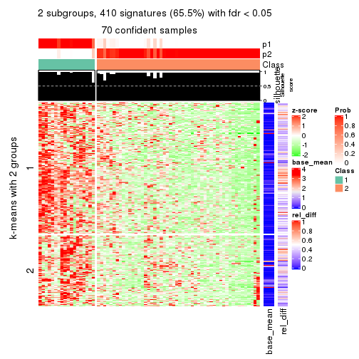
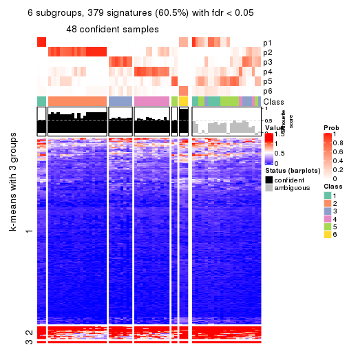
As soon as we have had the classes for columns, we can look for signatures which are significantly different between classes which can be candidate marks for certain classes. Following are the heatmaps for signatures.
Signature heatmaps where rows are scaled:
get_signatures(res, k = 2)
get_signatures(res, k = 3)
get_signatures(res, k = 4)
get_signatures(res, k = 5)
get_signatures(res, k = 6)
Signature heatmaps where rows are not scaled:
get_signatures(res, k = 2, scale_rows = FALSE)
get_signatures(res, k = 3, scale_rows = FALSE)
get_signatures(res, k = 4, scale_rows = FALSE)
get_signatures(res, k = 5, scale_rows = FALSE)
get_signatures(res, k = 6, scale_rows = FALSE)
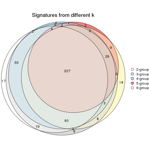
Compare the overlap of signatures from different k:
compare_signatures(res)
get_signature() returns a data frame invisibly. TO get the list of signatures, the function
call should be assigned to a variable explicitly. In following code, if plot argument is set
to FALSE, no heatmap is plotted while only the differential analysis is performed.
# code only for demonstration
tb = get_signature(res, k = ..., plot = FALSE)
An example of the output of tb is:
#>   which_row         fdr    mean_1    mean_2 scaled_mean_1 scaled_mean_2 km
#> 1        38 0.042760348  8.373488  9.131774    -0.5533452     0.5164555  1
#> 2        40 0.018707592  7.106213  8.469186    -0.6173731     0.5762149  1
#> 3        55 0.019134737 10.221463 11.207825    -0.6159697     0.5749050  1
#> 4        59 0.006059896  5.921854  7.869574    -0.6899429     0.6439467  1
#> 5        60 0.018055526  8.928898 10.211722    -0.6204761     0.5791110  1
#> 6        98 0.009384629 15.714769 14.887706     0.6635654    -0.6193277  2
...
The columns in tb are:
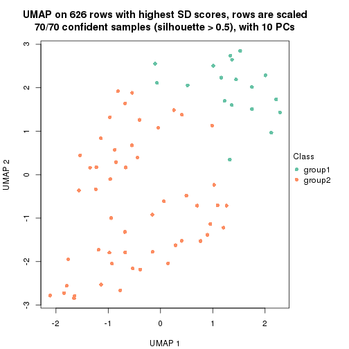
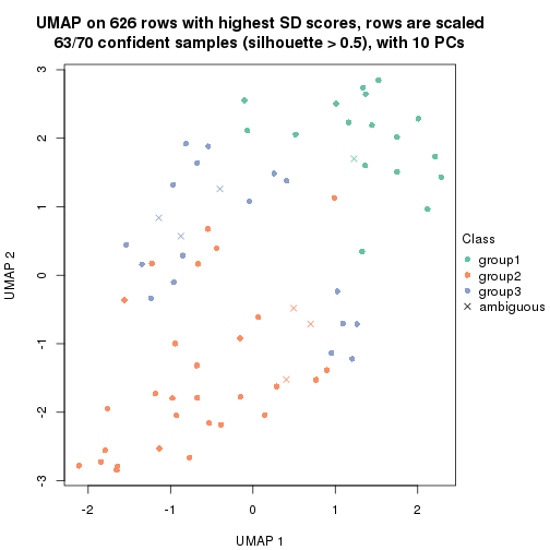
which_row: row indices corresponding to the input matrix.fdr: FDR for the differential test. mean_x: The mean value in group x.scaled_mean_x: The mean value in group x after rows are scaled.km: Row groups if k-means clustering is applied to rows.UMAP plot which shows how samples are separated.
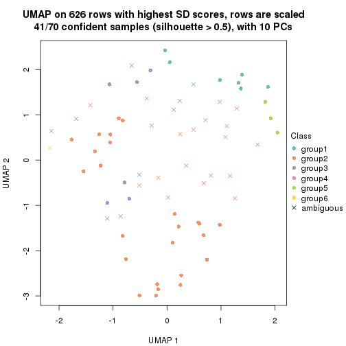
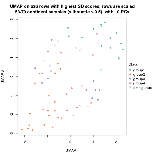
dimension_reduction(res, k = 2, method = "UMAP")
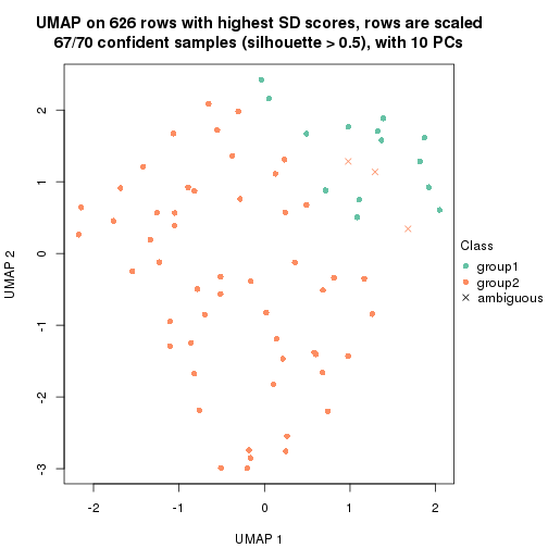
dimension_reduction(res, k = 3, method = "UMAP")
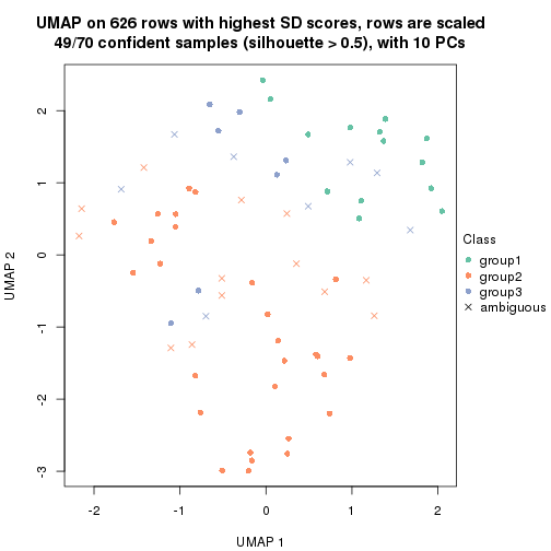
dimension_reduction(res, k = 4, method = "UMAP")
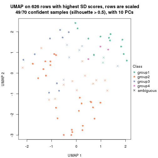
dimension_reduction(res, k = 5, method = "UMAP")
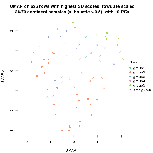
dimension_reduction(res, k = 6, method = "UMAP")
Following heatmap shows how subgroups are split when increasing k:
collect_classes(res)
If matrix rows can be associated to genes, consider to use functional_enrichment(res,
...) to perform function enrichment for the signature genes. See this vignette for more detailed explanations.
The object with results only for a single top-value method and a single partition method can be extracted as:
res = res_list["SD", "kmeans"]
# you can also extract it by
# res = res_list["SD:kmeans"]
A summary of res and all the functions that can be applied to it:
res
#> A 'ConsensusPartition' object with k = 2, 3, 4, 5, 6.
#>   On a matrix with 626 rows and 70 columns.
#>   Top rows (63, 126, 188, 250, 313) are extracted by 'SD' method.
#>   Subgroups are detected by 'kmeans' method.
#>   Performed in total 1250 partitions by row resampling.
#>   Best k for subgroups seems to be 2.
#>
#> Following methods can be applied to this 'ConsensusPartition' object:
#>  [1] "cola_report"             "collect_classes"         "collect_plots"
#>  [4] "collect_stats"           "colnames"                "compare_signatures"
#>  [7] "consensus_heatmap"       "dimension_reduction"     "functional_enrichment"
#> [10] "get_anno_col"            "get_anno"                "get_classes"
#> [13] "get_consensus"           "get_matrix"              "get_membership"
#> [16] "get_param"               "get_signatures"          "get_stats"
#> [19] "is_best_k"               "is_stable_k"             "membership_heatmap"
#> [22] "ncol"                    "nrow"                    "plot_ecdf"
#> [25] "rownames"                "select_partition_number" "show"
#> [28] "suggest_best_k"          "test_to_known_factors"
collect_plots() function collects all the plots made from res for all k (number of partitions)
into one single page to provide an easy and fast comparison between different k.
collect_plots(res)
The plots are:
k and the heatmap of
predicted classes for each k.k.k.k.All the plots in panels can be made by individual functions and they are plotted later in this section.
select_partition_number() produces several plots showing different
statistics for choosing “optimized” k. There are following statistics:
k;k, the area increased is defined as \(A_k - A_{k-1}\).The detailed explanations of these statistics can be found in the cola vignette.
Generally speaking, lower PAC score, higher mean silhouette score or higher
concordance corresponds to better partition. Rand index and Jaccard index
measure how similar the current partition is compared to partition with k-1.
If they are too similar, we won't accept k is better than k-1.
select_partition_number(res)
The numeric values for all these statistics can be obtained by get_stats().
get_stats(res)
#>   k 1-PAC mean_silhouette concordance area_increased  Rand Jaccard
#> 2 2 0.966           0.954       0.978         0.3971 0.612   0.612
#> 3 3 0.508           0.715       0.841         0.5834 0.735   0.567
#> 4 4 0.547           0.616       0.783         0.1417 0.851   0.604
#> 5 5 0.493           0.465       0.663         0.0675 0.867   0.569
#> 6 6 0.600           0.551       0.692         0.0441 0.891   0.584
suggest_best_k() suggests the best \(k\) based on these statistics. The rules are as follows:
suggest_best_k(res)
#> [1] 2
Following shows the table of the partitions (You need to click the show/hide
code output link to see it). The membership matrix (columns with name p*)
is inferred by
clue::cl_consensus()
function with the SE method. Basically the value in the membership matrix
represents the probability to belong to a certain group. The finall class
label for an item is determined with the group with highest probability it
belongs to.
In get_classes() function, the entropy is calculated from the membership
matrix and the silhouette score is calculated from the consensus matrix.
cbind(get_classes(res, k = 2), get_membership(res, k = 2))
#>           class entropy silhouette    p1    p2
#> SRR837437     2  0.0000      0.977 0.000 1.000
#> SRR837438     2  0.3431      0.929 0.064 0.936
#> SRR837439     2  0.0000      0.977 0.000 1.000
#> SRR837440     2  0.0000      0.977 0.000 1.000
#> SRR837441     2  0.0000      0.977 0.000 1.000
#> SRR837442     2  0.0000      0.977 0.000 1.000
#> SRR837443     2  0.0000      0.977 0.000 1.000
#> SRR837444     2  0.0000      0.977 0.000 1.000
#> SRR837445     2  0.0000      0.977 0.000 1.000
#> SRR837446     2  0.0000      0.977 0.000 1.000
#> SRR837447     1  0.0000      0.978 1.000 0.000
#> SRR837448     1  0.0000      0.978 1.000 0.000
#> SRR837449     1  0.0000      0.978 1.000 0.000
#> SRR837450     1  0.0000      0.978 1.000 0.000
#> SRR837451     2  0.0000      0.977 0.000 1.000
#> SRR837452     2  0.0000      0.977 0.000 1.000
#> SRR837453     2  0.0000      0.977 0.000 1.000
#> SRR837454     2  0.0000      0.977 0.000 1.000
#> SRR837455     1  0.0000      0.978 1.000 0.000
#> SRR837456     1  0.0000      0.978 1.000 0.000
#> SRR837457     2  0.0000      0.977 0.000 1.000
#> SRR837458     1  0.0000      0.978 1.000 0.000
#> SRR837459     2  0.0000      0.977 0.000 1.000
#> SRR837460     2  0.0000      0.977 0.000 1.000
#> SRR837461     2  0.0000      0.977 0.000 1.000
#> SRR837462     2  0.8207      0.684 0.256 0.744
#> SRR837463     2  0.3584      0.925 0.068 0.932
#> SRR837464     2  0.0000      0.977 0.000 1.000
#> SRR837465     2  0.1843      0.957 0.028 0.972
#> SRR837466     1  0.0000      0.978 1.000 0.000
#> SRR837467     2  0.0000      0.977 0.000 1.000
#> SRR837468     2  0.6247      0.832 0.156 0.844
#> SRR837469     1  0.0000      0.978 1.000 0.000
#> SRR837470     1  0.0000      0.978 1.000 0.000
#> SRR837471     2  0.0000      0.977 0.000 1.000
#> SRR837472     2  0.0000      0.977 0.000 1.000
#> SRR837473     2  0.3879      0.918 0.076 0.924
#> SRR837474     2  0.0000      0.977 0.000 1.000
#> SRR837475     2  0.0000      0.977 0.000 1.000
#> SRR837476     2  0.0000      0.977 0.000 1.000
#> SRR837477     2  0.6887      0.788 0.184 0.816
#> SRR837478     2  0.0000      0.977 0.000 1.000
#> SRR837479     2  0.0000      0.977 0.000 1.000
#> SRR837480     2  0.0000      0.977 0.000 1.000
#> SRR837481     2  0.0376      0.974 0.004 0.996
#> SRR837482     2  0.7376      0.756 0.208 0.792
#> SRR837483     1  0.0672      0.971 0.992 0.008
#> SRR837484     2  0.0000      0.977 0.000 1.000
#> SRR837485     2  0.0000      0.977 0.000 1.000
#> SRR837486     2  0.1843      0.958 0.028 0.972
#> SRR837487     2  0.0000      0.977 0.000 1.000
#> SRR837488     2  0.0000      0.977 0.000 1.000
#> SRR837489     2  0.0000      0.977 0.000 1.000
#> SRR837490     2  0.0000      0.977 0.000 1.000
#> SRR837491     2  0.0000      0.977 0.000 1.000
#> SRR837492     2  0.2236      0.953 0.036 0.964
#> SRR837493     2  0.3584      0.925 0.068 0.932
#> SRR837494     2  0.0000      0.977 0.000 1.000
#> SRR837495     2  0.0376      0.974 0.004 0.996
#> SRR837496     1  0.0000      0.978 1.000 0.000
#> SRR837497     1  0.0000      0.978 1.000 0.000
#> SRR837498     1  0.0000      0.978 1.000 0.000
#> SRR837499     1  0.0000      0.978 1.000 0.000
#> SRR837500     1  0.4298      0.893 0.912 0.088
#> SRR837501     2  0.0000      0.977 0.000 1.000
#> SRR837502     1  0.8327      0.627 0.736 0.264
#> SRR837503     1  0.0000      0.978 1.000 0.000
#> SRR837504     2  0.0000      0.977 0.000 1.000
#> SRR837505     2  0.0000      0.977 0.000 1.000
#> SRR837506     2  0.0000      0.977 0.000 1.000
cbind(get_classes(res, k = 3), get_membership(res, k = 3))
#>           class entropy silhouette    p1    p2    p3
#> SRR837437     2  0.1031      0.832 0.000 0.976 0.024
#> SRR837438     3  0.5357      0.714 0.064 0.116 0.820
#> SRR837439     2  0.4452      0.641 0.000 0.808 0.192
#> SRR837440     3  0.6302      0.456 0.000 0.480 0.520
#> SRR837441     2  0.4452      0.627 0.000 0.808 0.192
#> SRR837442     2  0.0237      0.839 0.000 0.996 0.004
#> SRR837443     3  0.6126      0.606 0.000 0.400 0.600
#> SRR837444     3  0.3412      0.748 0.000 0.124 0.876
#> SRR837445     2  0.5560      0.539 0.000 0.700 0.300
#> SRR837446     3  0.5591      0.698 0.000 0.304 0.696
#> SRR837447     1  0.0237      0.877 0.996 0.000 0.004
#> SRR837448     1  0.2711      0.851 0.912 0.000 0.088
#> SRR837449     1  0.3192      0.862 0.888 0.000 0.112
#> SRR837450     1  0.2711      0.851 0.912 0.000 0.088
#> SRR837451     2  0.0424      0.839 0.000 0.992 0.008
#> SRR837452     2  0.0424      0.839 0.000 0.992 0.008
#> SRR837453     2  0.0424      0.839 0.000 0.992 0.008
#> SRR837454     2  0.0000      0.839 0.000 1.000 0.000
#> SRR837455     1  0.0592      0.877 0.988 0.000 0.012
#> SRR837456     1  0.0592      0.877 0.988 0.000 0.012
#> SRR837457     2  0.0424      0.839 0.000 0.992 0.008
#> SRR837458     1  0.1643      0.870 0.956 0.000 0.044
#> SRR837459     2  0.0424      0.839 0.000 0.992 0.008
#> SRR837460     2  0.0424      0.839 0.000 0.992 0.008
#> SRR837461     3  0.6307      0.431 0.000 0.488 0.512
#> SRR837462     3  0.3590      0.692 0.076 0.028 0.896
#> SRR837463     3  0.4379      0.720 0.060 0.072 0.868
#> SRR837464     3  0.4887      0.751 0.000 0.228 0.772
#> SRR837465     3  0.7391      0.488 0.056 0.308 0.636
#> SRR837466     1  0.2711      0.851 0.912 0.000 0.088
#> SRR837467     2  0.1289      0.827 0.000 0.968 0.032
#> SRR837468     3  0.3406      0.695 0.068 0.028 0.904
#> SRR837469     1  0.0747      0.876 0.984 0.000 0.016
#> SRR837470     1  0.0747      0.876 0.984 0.000 0.016
#> SRR837471     2  0.0424      0.837 0.000 0.992 0.008
#> SRR837472     2  0.0424      0.837 0.000 0.992 0.008
#> SRR837473     2  0.6441      0.532 0.028 0.696 0.276
#> SRR837474     2  0.0424      0.837 0.000 0.992 0.008
#> SRR837475     2  0.0424      0.837 0.000 0.992 0.008
#> SRR837476     2  0.0000      0.839 0.000 1.000 0.000
#> SRR837477     2  0.8085      0.168 0.068 0.520 0.412
#> SRR837478     2  0.3752      0.732 0.000 0.856 0.144
#> SRR837479     3  0.5254      0.728 0.000 0.264 0.736
#> SRR837480     2  0.4555      0.667 0.000 0.800 0.200
#> SRR837481     3  0.4842      0.749 0.000 0.224 0.776
#> SRR837482     3  0.3337      0.704 0.060 0.032 0.908
#> SRR837483     1  0.6140      0.571 0.596 0.000 0.404
#> SRR837484     2  0.6045      0.156 0.000 0.620 0.380
#> SRR837485     2  0.6280     -0.191 0.000 0.540 0.460
#> SRR837486     3  0.3340      0.754 0.000 0.120 0.880
#> SRR837487     2  0.0424      0.839 0.000 0.992 0.008
#> SRR837488     2  0.0424      0.839 0.000 0.992 0.008
#> SRR837489     2  0.0424      0.837 0.000 0.992 0.008
#> SRR837490     2  0.0237      0.838 0.000 0.996 0.004
#> SRR837491     2  0.5560      0.518 0.000 0.700 0.300
#> SRR837492     2  0.5884      0.562 0.012 0.716 0.272
#> SRR837493     3  0.5229      0.709 0.068 0.104 0.828
#> SRR837494     2  0.1163      0.829 0.000 0.972 0.028
#> SRR837495     2  0.5216      0.599 0.000 0.740 0.260
#> SRR837496     1  0.2711      0.873 0.912 0.000 0.088
#> SRR837497     1  0.2537      0.871 0.920 0.000 0.080
#> SRR837498     1  0.3340      0.857 0.880 0.000 0.120
#> SRR837499     1  0.4399      0.810 0.812 0.000 0.188
#> SRR837500     1  0.7941      0.605 0.628 0.096 0.276
#> SRR837501     3  0.4702      0.753 0.000 0.212 0.788
#> SRR837502     1  0.7187      0.292 0.496 0.024 0.480
#> SRR837503     1  0.3340      0.861 0.880 0.000 0.120
#> SRR837504     3  0.6062      0.619 0.000 0.384 0.616
#> SRR837505     3  0.5926      0.645 0.000 0.356 0.644
#> SRR837506     3  0.5882      0.654 0.000 0.348 0.652
cbind(get_classes(res, k = 4), get_membership(res, k = 4))
#>           class entropy silhouette    p1    p2    p3    p4
#> SRR837437     2  0.1520      0.846 0.000 0.956 0.024 0.020
#> SRR837438     4  0.6552      0.255 0.032 0.028 0.396 0.544
#> SRR837439     2  0.5905      0.527 0.000 0.700 0.144 0.156
#> SRR837440     3  0.7206      0.342 0.000 0.400 0.460 0.140
#> SRR837441     2  0.5722      0.552 0.000 0.716 0.136 0.148
#> SRR837442     2  0.0469      0.858 0.000 0.988 0.000 0.012
#> SRR837443     3  0.7143      0.374 0.000 0.380 0.484 0.136
#> SRR837444     4  0.5894      0.186 0.000 0.036 0.428 0.536
#> SRR837445     4  0.5791      0.571 0.000 0.284 0.060 0.656
#> SRR837446     3  0.5159      0.641 0.000 0.156 0.756 0.088
#> SRR837447     1  0.0921      0.785 0.972 0.000 0.000 0.028
#> SRR837448     1  0.3991      0.724 0.808 0.000 0.020 0.172
#> SRR837449     1  0.4769      0.633 0.684 0.000 0.008 0.308
#> SRR837450     1  0.4035      0.725 0.804 0.000 0.020 0.176
#> SRR837451     2  0.0188      0.858 0.000 0.996 0.004 0.000
#> SRR837452     2  0.2589      0.809 0.000 0.884 0.000 0.116
#> SRR837453     2  0.0188      0.858 0.000 0.996 0.004 0.000
#> SRR837454     2  0.0188      0.858 0.000 0.996 0.004 0.000
#> SRR837455     1  0.1576      0.785 0.948 0.000 0.004 0.048
#> SRR837456     1  0.1576      0.785 0.948 0.000 0.004 0.048
#> SRR837457     2  0.0188      0.858 0.000 0.996 0.004 0.000
#> SRR837458     1  0.1209      0.781 0.964 0.000 0.004 0.032
#> SRR837459     2  0.0188      0.858 0.000 0.996 0.004 0.000
#> SRR837460     2  0.0188      0.858 0.000 0.996 0.004 0.000
#> SRR837461     3  0.6903      0.397 0.000 0.380 0.508 0.112
#> SRR837462     3  0.5540      0.352 0.028 0.004 0.648 0.320
#> SRR837463     3  0.5488      0.337 0.012 0.012 0.636 0.340
#> SRR837464     3  0.5307      0.561 0.000 0.076 0.736 0.188
#> SRR837465     4  0.6585      0.520 0.012 0.120 0.212 0.656
#> SRR837466     1  0.3991      0.724 0.808 0.000 0.020 0.172
#> SRR837467     2  0.1520      0.846 0.000 0.956 0.020 0.024
#> SRR837468     3  0.1771      0.674 0.012 0.004 0.948 0.036
#> SRR837469     1  0.1576      0.781 0.948 0.000 0.004 0.048
#> SRR837470     1  0.1576      0.780 0.948 0.000 0.004 0.048
#> SRR837471     2  0.2760      0.802 0.000 0.872 0.000 0.128
#> SRR837472     2  0.2149      0.825 0.000 0.912 0.000 0.088
#> SRR837473     4  0.6038      0.601 0.024 0.264 0.040 0.672
#> SRR837474     2  0.2589      0.811 0.000 0.884 0.000 0.116
#> SRR837475     2  0.2281      0.818 0.000 0.904 0.000 0.096
#> SRR837476     2  0.1004      0.857 0.000 0.972 0.004 0.024
#> SRR837477     4  0.7114      0.489 0.004 0.220 0.192 0.584
#> SRR837478     2  0.6854      0.444 0.000 0.600 0.204 0.196
#> SRR837479     3  0.2844      0.689 0.000 0.048 0.900 0.052
#> SRR837480     2  0.7133      0.346 0.000 0.548 0.280 0.172
#> SRR837481     3  0.2751      0.688 0.000 0.040 0.904 0.056
#> SRR837482     3  0.1771      0.675 0.012 0.004 0.948 0.036
#> SRR837483     1  0.7860      0.204 0.396 0.000 0.292 0.312
#> SRR837484     2  0.5407     -0.136 0.000 0.504 0.484 0.012
#> SRR837485     3  0.5233      0.501 0.000 0.332 0.648 0.020
#> SRR837486     3  0.1796      0.687 0.004 0.016 0.948 0.032
#> SRR837487     2  0.1489      0.852 0.000 0.952 0.004 0.044
#> SRR837488     2  0.0188      0.858 0.000 0.996 0.004 0.000
#> SRR837489     2  0.3074      0.785 0.000 0.848 0.000 0.152
#> SRR837490     2  0.0707      0.856 0.000 0.980 0.000 0.020
#> SRR837491     4  0.6638      0.276 0.000 0.420 0.084 0.496
#> SRR837492     4  0.5570      0.590 0.004 0.268 0.044 0.684
#> SRR837493     4  0.6739      0.209 0.040 0.028 0.412 0.520
#> SRR837494     2  0.1182      0.849 0.000 0.968 0.016 0.016
#> SRR837495     4  0.5619      0.525 0.000 0.320 0.040 0.640
#> SRR837496     1  0.5069      0.635 0.664 0.000 0.016 0.320
#> SRR837497     1  0.4422      0.702 0.736 0.000 0.008 0.256
#> SRR837498     1  0.4482      0.694 0.728 0.000 0.008 0.264
#> SRR837499     4  0.5511     -0.320 0.484 0.000 0.016 0.500
#> SRR837500     4  0.4978      0.363 0.240 0.016 0.012 0.732
#> SRR837501     3  0.1820      0.697 0.000 0.036 0.944 0.020
#> SRR837502     4  0.5710      0.417 0.204 0.008 0.072 0.716
#> SRR837503     1  0.5217      0.552 0.608 0.000 0.012 0.380
#> SRR837504     3  0.5157      0.585 0.000 0.284 0.688 0.028
#> SRR837505     3  0.2775      0.700 0.000 0.084 0.896 0.020
#> SRR837506     3  0.2909      0.696 0.000 0.092 0.888 0.020
cbind(get_classes(res, k = 5), get_membership(res, k = 5))
#>           class entropy silhouette    p1    p2    p3    p4    p5
#> SRR837437     2  0.3759   0.679752 0.000 0.764 0.016 0.220 0.000
#> SRR837438     4  0.5162   0.404744 0.140 0.004 0.152 0.704 0.000
#> SRR837439     4  0.5548   0.125681 0.000 0.440 0.068 0.492 0.000
#> SRR837440     4  0.6602   0.263095 0.000 0.260 0.240 0.496 0.004
#> SRR837441     4  0.5548   0.125681 0.000 0.440 0.068 0.492 0.000
#> SRR837442     2  0.2179   0.816163 0.000 0.896 0.004 0.100 0.000
#> SRR837443     4  0.6605   0.257138 0.000 0.252 0.248 0.496 0.004
#> SRR837444     4  0.5093   0.381145 0.088 0.000 0.164 0.728 0.020
#> SRR837445     4  0.7086   0.373266 0.132 0.152 0.020 0.612 0.084
#> SRR837446     3  0.5936   0.532173 0.000 0.080 0.656 0.216 0.048
#> SRR837447     1  0.4517  -0.036550 0.616 0.000 0.004 0.008 0.372
#> SRR837448     5  0.3074   0.988151 0.196 0.000 0.000 0.000 0.804
#> SRR837449     1  0.2914   0.441768 0.872 0.000 0.000 0.076 0.052
#> SRR837450     5  0.3143   0.982294 0.204 0.000 0.000 0.000 0.796
#> SRR837451     2  0.0404   0.825891 0.000 0.988 0.000 0.000 0.012
#> SRR837452     2  0.3452   0.789287 0.000 0.820 0.000 0.148 0.032
#> SRR837453     2  0.0404   0.825891 0.000 0.988 0.000 0.000 0.012
#> SRR837454     2  0.0404   0.825891 0.000 0.988 0.000 0.000 0.012
#> SRR837455     1  0.4552  -0.000993 0.632 0.000 0.004 0.012 0.352
#> SRR837456     1  0.4552  -0.000993 0.632 0.000 0.004 0.012 0.352
#> SRR837457     2  0.0404   0.825891 0.000 0.988 0.000 0.000 0.012
#> SRR837458     1  0.4855  -0.218695 0.544 0.000 0.004 0.016 0.436
#> SRR837459     2  0.0404   0.825891 0.000 0.988 0.000 0.000 0.012
#> SRR837460     2  0.0404   0.825891 0.000 0.988 0.000 0.000 0.012
#> SRR837461     4  0.6955   0.129237 0.000 0.228 0.332 0.428 0.012
#> SRR837462     4  0.6041   0.008587 0.056 0.000 0.412 0.504 0.028
#> SRR837463     4  0.5786   0.094975 0.048 0.004 0.384 0.548 0.016
#> SRR837464     3  0.5556   0.029799 0.004 0.028 0.496 0.456 0.016
#> SRR837465     4  0.5127   0.454832 0.120 0.028 0.076 0.760 0.016
#> SRR837466     5  0.3109   0.986651 0.200 0.000 0.000 0.000 0.800
#> SRR837467     2  0.3563   0.702179 0.000 0.780 0.012 0.208 0.000
#> SRR837468     3  0.3735   0.639882 0.008 0.000 0.828 0.100 0.064
#> SRR837469     1  0.5315  -0.200293 0.500 0.000 0.004 0.040 0.456
#> SRR837470     1  0.5320  -0.230974 0.488 0.000 0.004 0.040 0.468
#> SRR837471     2  0.3655   0.782116 0.000 0.804 0.000 0.160 0.036
#> SRR837472     2  0.3146   0.802501 0.000 0.844 0.000 0.128 0.028
#> SRR837473     4  0.7418   0.236885 0.292 0.152 0.004 0.488 0.064
#> SRR837474     2  0.3452   0.793403 0.000 0.820 0.000 0.148 0.032
#> SRR837475     2  0.2300   0.798918 0.000 0.904 0.000 0.072 0.024
#> SRR837476     2  0.2124   0.820809 0.000 0.900 0.004 0.096 0.000
#> SRR837477     4  0.9096   0.156696 0.232 0.100 0.144 0.408 0.116
#> SRR837478     2  0.8053   0.163315 0.004 0.432 0.228 0.232 0.104
#> SRR837479     3  0.3105   0.661096 0.000 0.004 0.864 0.088 0.044
#> SRR837480     2  0.8184   0.065878 0.004 0.380 0.280 0.236 0.100
#> SRR837481     3  0.3289   0.651483 0.000 0.000 0.844 0.108 0.048
#> SRR837482     3  0.3265   0.668217 0.008 0.000 0.856 0.096 0.040
#> SRR837483     1  0.7385   0.177859 0.464 0.000 0.324 0.136 0.076
#> SRR837484     3  0.5412   0.184112 0.000 0.428 0.520 0.048 0.004
#> SRR837485     3  0.5246   0.473658 0.000 0.260 0.672 0.044 0.024
#> SRR837486     3  0.1300   0.684500 0.000 0.000 0.956 0.028 0.016
#> SRR837487     2  0.2396   0.827595 0.000 0.904 0.004 0.068 0.024
#> SRR837488     2  0.0404   0.825891 0.000 0.988 0.000 0.000 0.012
#> SRR837489     2  0.3562   0.753435 0.000 0.788 0.000 0.196 0.016
#> SRR837490     2  0.1608   0.828213 0.000 0.928 0.000 0.072 0.000
#> SRR837491     4  0.5948   0.429019 0.040 0.260 0.040 0.644 0.016
#> SRR837492     4  0.7979   0.243762 0.244 0.140 0.032 0.500 0.084
#> SRR837493     4  0.5150   0.394038 0.128 0.004 0.164 0.704 0.000
#> SRR837494     2  0.3239   0.741084 0.000 0.828 0.012 0.156 0.004
#> SRR837495     4  0.7868   0.279279 0.216 0.180 0.016 0.500 0.088
#> SRR837496     1  0.3681   0.434050 0.808 0.000 0.000 0.148 0.044
#> SRR837497     1  0.3857   0.418719 0.808 0.000 0.000 0.084 0.108
#> SRR837498     1  0.4480   0.392802 0.772 0.000 0.008 0.092 0.128
#> SRR837499     1  0.3366   0.433786 0.768 0.000 0.000 0.232 0.000
#> SRR837500     1  0.5447   0.173394 0.552 0.012 0.000 0.396 0.040
#> SRR837501     3  0.2654   0.663877 0.000 0.000 0.884 0.084 0.032
#> SRR837502     1  0.5844   0.126180 0.524 0.008 0.020 0.412 0.036
#> SRR837503     1  0.3081   0.450203 0.832 0.000 0.000 0.156 0.012
#> SRR837504     3  0.6906   0.168557 0.000 0.232 0.480 0.272 0.016
#> SRR837505     3  0.3068   0.680558 0.000 0.036 0.880 0.056 0.028
#> SRR837506     3  0.2532   0.687369 0.000 0.036 0.908 0.028 0.028
cbind(get_classes(res, k = 6), get_membership(res, k = 6))
#>           class entropy silhouette    p1    p2    p3    p4    p5    p6
#> SRR837437     2  0.3534     0.5915 0.000 0.716 0.008 0.276 0.000 0.000
#> SRR837438     4  0.3789     0.5521 0.000 0.004 0.016 0.784 0.168 0.028
#> SRR837439     4  0.4365     0.5375 0.000 0.332 0.008 0.636 0.024 0.000
#> SRR837440     4  0.4857     0.6302 0.000 0.256 0.044 0.672 0.020 0.008
#> SRR837441     4  0.4379     0.5319 0.000 0.336 0.008 0.632 0.024 0.000
#> SRR837442     2  0.2560     0.8099 0.000 0.872 0.000 0.092 0.036 0.000
#> SRR837443     4  0.4833     0.6145 0.000 0.272 0.048 0.656 0.024 0.000
#> SRR837444     4  0.5564     0.4076 0.000 0.004 0.128 0.620 0.228 0.020
#> SRR837445     5  0.5600     0.4139 0.000 0.076 0.088 0.168 0.664 0.004
#> SRR837446     3  0.5384     0.4923 0.000 0.060 0.688 0.112 0.136 0.004
#> SRR837447     1  0.1321     0.5225 0.952 0.000 0.000 0.004 0.024 0.020
#> SRR837448     6  0.3890     0.9879 0.400 0.000 0.000 0.000 0.004 0.596
#> SRR837449     1  0.5803     0.3208 0.576 0.000 0.000 0.080 0.288 0.056
#> SRR837450     6  0.3984     0.9857 0.396 0.000 0.000 0.000 0.008 0.596
#> SRR837451     2  0.1296     0.8225 0.000 0.948 0.004 0.000 0.004 0.044
#> SRR837452     2  0.3812     0.7538 0.000 0.760 0.004 0.024 0.204 0.008
#> SRR837453     2  0.1296     0.8225 0.000 0.948 0.004 0.000 0.004 0.044
#> SRR837454     2  0.1296     0.8225 0.000 0.948 0.004 0.000 0.004 0.044
#> SRR837455     1  0.0972     0.5102 0.964 0.000 0.000 0.000 0.008 0.028
#> SRR837456     1  0.0972     0.5102 0.964 0.000 0.000 0.000 0.008 0.028
#> SRR837457     2  0.1296     0.8225 0.000 0.948 0.004 0.000 0.004 0.044
#> SRR837458     1  0.1913     0.4657 0.920 0.000 0.004 0.004 0.012 0.060
#> SRR837459     2  0.1296     0.8225 0.000 0.948 0.004 0.000 0.004 0.044
#> SRR837460     2  0.1296     0.8225 0.000 0.948 0.004 0.000 0.004 0.044
#> SRR837461     4  0.4588     0.6230 0.000 0.228 0.048 0.700 0.000 0.024
#> SRR837462     4  0.4222     0.5067 0.004 0.000 0.092 0.784 0.032 0.088
#> SRR837463     4  0.2945     0.5798 0.000 0.000 0.072 0.864 0.016 0.048
#> SRR837464     4  0.3813     0.5360 0.000 0.012 0.132 0.800 0.008 0.048
#> SRR837465     4  0.3949     0.5309 0.000 0.020 0.000 0.744 0.216 0.020
#> SRR837466     6  0.3899     0.9820 0.404 0.000 0.000 0.000 0.004 0.592
#> SRR837467     2  0.3489     0.5753 0.000 0.708 0.004 0.288 0.000 0.000
#> SRR837468     3  0.5897     0.5558 0.000 0.000 0.584 0.208 0.032 0.176
#> SRR837469     1  0.5267     0.3951 0.712 0.000 0.024 0.052 0.064 0.148
#> SRR837470     1  0.5154     0.3952 0.720 0.000 0.020 0.052 0.064 0.144
#> SRR837471     2  0.4413     0.7376 0.000 0.720 0.000 0.056 0.208 0.016
#> SRR837472     2  0.3750     0.7534 0.000 0.764 0.000 0.020 0.200 0.016
#> SRR837473     5  0.4652     0.5044 0.008 0.080 0.004 0.140 0.748 0.020
#> SRR837474     2  0.4298     0.7515 0.000 0.736 0.000 0.056 0.192 0.016
#> SRR837475     2  0.3364     0.7497 0.000 0.780 0.000 0.000 0.196 0.024
#> SRR837476     2  0.2443     0.8095 0.000 0.880 0.000 0.096 0.020 0.004
#> SRR837477     5  0.4684     0.3703 0.000 0.028 0.240 0.016 0.696 0.020
#> SRR837478     5  0.6548    -0.0932 0.000 0.248 0.364 0.012 0.368 0.008
#> SRR837479     3  0.2776     0.5752 0.000 0.000 0.860 0.032 0.104 0.004
#> SRR837480     3  0.6295     0.0315 0.000 0.200 0.428 0.012 0.356 0.004
#> SRR837481     3  0.2653     0.5747 0.000 0.000 0.868 0.028 0.100 0.004
#> SRR837482     3  0.3916     0.6153 0.000 0.000 0.792 0.128 0.028 0.052
#> SRR837483     3  0.8544    -0.0469 0.128 0.000 0.316 0.116 0.272 0.168
#> SRR837484     3  0.5065     0.2001 0.000 0.396 0.532 0.068 0.000 0.004
#> SRR837485     3  0.4785     0.4356 0.000 0.284 0.652 0.048 0.012 0.004
#> SRR837486     3  0.3900     0.6269 0.000 0.000 0.784 0.116 0.008 0.092
#> SRR837487     2  0.2726     0.8223 0.000 0.880 0.008 0.056 0.052 0.004
#> SRR837488     2  0.1296     0.8225 0.000 0.948 0.004 0.000 0.004 0.044
#> SRR837489     2  0.3742     0.7777 0.000 0.796 0.000 0.120 0.076 0.008
#> SRR837490     2  0.2138     0.8226 0.000 0.908 0.000 0.052 0.036 0.004
#> SRR837491     4  0.5497     0.5437 0.000 0.208 0.000 0.608 0.172 0.012
#> SRR837492     5  0.4497     0.5126 0.000 0.048 0.084 0.080 0.776 0.012
#> SRR837493     4  0.3646     0.5608 0.000 0.004 0.016 0.800 0.152 0.028
#> SRR837494     2  0.3081     0.6846 0.000 0.776 0.000 0.220 0.000 0.004
#> SRR837495     5  0.4882     0.4897 0.000 0.088 0.088 0.080 0.740 0.004
#> SRR837496     5  0.6213    -0.0674 0.364 0.000 0.004 0.052 0.488 0.092
#> SRR837497     1  0.6234     0.3612 0.524 0.000 0.000 0.064 0.304 0.108
#> SRR837498     1  0.6927     0.4399 0.516 0.000 0.008 0.124 0.216 0.136
#> SRR837499     5  0.6556     0.0953 0.320 0.000 0.000 0.132 0.476 0.072
#> SRR837500     5  0.5987     0.4123 0.120 0.000 0.000 0.204 0.604 0.072
#> SRR837501     3  0.5439     0.5728 0.000 0.000 0.624 0.204 0.016 0.156
#> SRR837502     5  0.6185     0.3939 0.112 0.000 0.000 0.256 0.560 0.072
#> SRR837503     5  0.6167    -0.0444 0.372 0.000 0.000 0.068 0.480 0.080
#> SRR837504     4  0.6373     0.2648 0.000 0.236 0.276 0.464 0.000 0.024
#> SRR837505     3  0.5049     0.6092 0.000 0.008 0.692 0.144 0.012 0.144
#> SRR837506     3  0.5042     0.6145 0.000 0.008 0.700 0.108 0.020 0.164
Heatmaps for the consensus matrix. It visualizes the probability of two samples to be in a same group.
consensus_heatmap(res, k = 2)
consensus_heatmap(res, k = 3)
consensus_heatmap(res, k = 4)
consensus_heatmap(res, k = 5)
consensus_heatmap(res, k = 6)
Heatmaps for the membership of samples in all partitions to see how consistent they are:
membership_heatmap(res, k = 2)
membership_heatmap(res, k = 3)
membership_heatmap(res, k = 4)
membership_heatmap(res, k = 5)
membership_heatmap(res, k = 6)
As soon as we have had the classes for columns, we can look for signatures which are significantly different between classes which can be candidate marks for certain classes. Following are the heatmaps for signatures.
Signature heatmaps where rows are scaled:
get_signatures(res, k = 2)
get_signatures(res, k = 3)
get_signatures(res, k = 4)
get_signatures(res, k = 5)
get_signatures(res, k = 6)
Signature heatmaps where rows are not scaled:
get_signatures(res, k = 2, scale_rows = FALSE)
get_signatures(res, k = 3, scale_rows = FALSE)
get_signatures(res, k = 4, scale_rows = FALSE)
get_signatures(res, k = 5, scale_rows = FALSE)
get_signatures(res, k = 6, scale_rows = FALSE)
Compare the overlap of signatures from different k:
compare_signatures(res)
get_signature() returns a data frame invisibly. TO get the list of signatures, the function
call should be assigned to a variable explicitly. In following code, if plot argument is set
to FALSE, no heatmap is plotted while only the differential analysis is performed.
# code only for demonstration
tb = get_signature(res, k = ..., plot = FALSE)
An example of the output of tb is:
#>   which_row         fdr    mean_1    mean_2 scaled_mean_1 scaled_mean_2 km
#> 1        38 0.042760348  8.373488  9.131774    -0.5533452     0.5164555  1
#> 2        40 0.018707592  7.106213  8.469186    -0.6173731     0.5762149  1
#> 3        55 0.019134737 10.221463 11.207825    -0.6159697     0.5749050  1
#> 4        59 0.006059896  5.921854  7.869574    -0.6899429     0.6439467  1
#> 5        60 0.018055526  8.928898 10.211722    -0.6204761     0.5791110  1
#> 6        98 0.009384629 15.714769 14.887706     0.6635654    -0.6193277  2
...
The columns in tb are:
which_row: row indices corresponding to the input matrix.fdr: FDR for the differential test. mean_x: The mean value in group x.scaled_mean_x: The mean value in group x after rows are scaled.km: Row groups if k-means clustering is applied to rows.UMAP plot which shows how samples are separated.
dimension_reduction(res, k = 2, method = "UMAP")
dimension_reduction(res, k = 3, method = "UMAP")
dimension_reduction(res, k = 4, method = "UMAP")
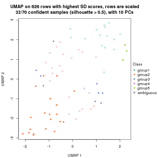
dimension_reduction(res, k = 5, method = "UMAP")
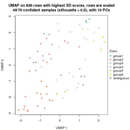
dimension_reduction(res, k = 6, method = "UMAP")
Following heatmap shows how subgroups are split when increasing k:
collect_classes(res)
If matrix rows can be associated to genes, consider to use functional_enrichment(res,
...) to perform function enrichment for the signature genes. See this vignette for more detailed explanations.
The object with results only for a single top-value method and a single partition method can be extracted as:
res = res_list["SD", "skmeans"]
# you can also extract it by
# res = res_list["SD:skmeans"]
A summary of res and all the functions that can be applied to it:
res
#> A 'ConsensusPartition' object with k = 2, 3, 4, 5, 6.
#>   On a matrix with 626 rows and 70 columns.
#>   Top rows (63, 126, 188, 250, 313) are extracted by 'SD' method.
#>   Subgroups are detected by 'skmeans' method.
#>   Performed in total 1250 partitions by row resampling.
#>   Best k for subgroups seems to be 2.
#>
#> Following methods can be applied to this 'ConsensusPartition' object:
#>  [1] "cola_report"             "collect_classes"         "collect_plots"
#>  [4] "collect_stats"           "colnames"                "compare_signatures"
#>  [7] "consensus_heatmap"       "dimension_reduction"     "functional_enrichment"
#> [10] "get_anno_col"            "get_anno"                "get_classes"
#> [13] "get_consensus"           "get_matrix"              "get_membership"
#> [16] "get_param"               "get_signatures"          "get_stats"
#> [19] "is_best_k"               "is_stable_k"             "membership_heatmap"
#> [22] "ncol"                    "nrow"                    "plot_ecdf"
#> [25] "rownames"                "select_partition_number" "show"
#> [28] "suggest_best_k"          "test_to_known_factors"
collect_plots() function collects all the plots made from res for all k (number of partitions)
into one single page to provide an easy and fast comparison between different k.
collect_plots(res)
The plots are:
k and the heatmap of
predicted classes for each k.k.k.k.All the plots in panels can be made by individual functions and they are plotted later in this section.
select_partition_number() produces several plots showing different
statistics for choosing “optimized” k. There are following statistics:
k;k, the area increased is defined as \(A_k - A_{k-1}\).The detailed explanations of these statistics can be found in the cola vignette.
Generally speaking, lower PAC score, higher mean silhouette score or higher
concordance corresponds to better partition. Rand index and Jaccard index
measure how similar the current partition is compared to partition with k-1.
If they are too similar, we won't accept k is better than k-1.
select_partition_number(res)
The numeric values for all these statistics can be obtained by get_stats().
get_stats(res)
#>   k 1-PAC mean_silhouette concordance area_increased  Rand Jaccard
#> 2 2 0.966           0.962       0.981         0.4954 0.503   0.503
#> 3 3 0.752           0.847       0.928         0.3377 0.763   0.557
#> 4 4 0.698           0.665       0.804         0.1103 0.858   0.610
#> 5 5 0.705           0.731       0.842         0.0659 0.955   0.827
#> 6 6 0.716           0.621       0.776         0.0367 0.967   0.853
suggest_best_k() suggests the best \(k\) based on these statistics. The rules are as follows:
suggest_best_k(res)
#> [1] 2
Following shows the table of the partitions (You need to click the show/hide
code output link to see it). The membership matrix (columns with name p*)
is inferred by
clue::cl_consensus()
function with the SE method. Basically the value in the membership matrix
represents the probability to belong to a certain group. The finall class
label for an item is determined with the group with highest probability it
belongs to.
In get_classes() function, the entropy is calculated from the membership
matrix and the silhouette score is calculated from the consensus matrix.
cbind(get_classes(res, k = 2), get_membership(res, k = 2))
#>           class entropy silhouette    p1    p2
#> SRR837437     2  0.0000      0.988 0.000 1.000
#> SRR837438     1  0.0672      0.966 0.992 0.008
#> SRR837439     2  0.0000      0.988 0.000 1.000
#> SRR837440     2  0.0000      0.988 0.000 1.000
#> SRR837441     2  0.0000      0.988 0.000 1.000
#> SRR837442     2  0.0000      0.988 0.000 1.000
#> SRR837443     2  0.0000      0.988 0.000 1.000
#> SRR837444     1  0.8661      0.613 0.712 0.288
#> SRR837445     2  0.4562      0.895 0.096 0.904
#> SRR837446     2  0.0000      0.988 0.000 1.000
#> SRR837447     1  0.0000      0.970 1.000 0.000
#> SRR837448     1  0.0000      0.970 1.000 0.000
#> SRR837449     1  0.0000      0.970 1.000 0.000
#> SRR837450     1  0.0000      0.970 1.000 0.000
#> SRR837451     2  0.0000      0.988 0.000 1.000
#> SRR837452     2  0.0000      0.988 0.000 1.000
#> SRR837453     2  0.0000      0.988 0.000 1.000
#> SRR837454     2  0.0000      0.988 0.000 1.000
#> SRR837455     1  0.0000      0.970 1.000 0.000
#> SRR837456     1  0.0000      0.970 1.000 0.000
#> SRR837457     2  0.0000      0.988 0.000 1.000
#> SRR837458     1  0.0000      0.970 1.000 0.000
#> SRR837459     2  0.0000      0.988 0.000 1.000
#> SRR837460     2  0.0000      0.988 0.000 1.000
#> SRR837461     2  0.0000      0.988 0.000 1.000
#> SRR837462     1  0.0000      0.970 1.000 0.000
#> SRR837463     1  0.2043      0.950 0.968 0.032
#> SRR837464     2  0.0376      0.985 0.004 0.996
#> SRR837465     1  0.6247      0.829 0.844 0.156
#> SRR837466     1  0.0000      0.970 1.000 0.000
#> SRR837467     2  0.0000      0.988 0.000 1.000
#> SRR837468     1  0.0000      0.970 1.000 0.000
#> SRR837469     1  0.0000      0.970 1.000 0.000
#> SRR837470     1  0.0000      0.970 1.000 0.000
#> SRR837471     2  0.0000      0.988 0.000 1.000
#> SRR837472     2  0.0000      0.988 0.000 1.000
#> SRR837473     1  0.1184      0.961 0.984 0.016
#> SRR837474     2  0.0000      0.988 0.000 1.000
#> SRR837475     2  0.0000      0.988 0.000 1.000
#> SRR837476     2  0.0000      0.988 0.000 1.000
#> SRR837477     1  0.4161      0.905 0.916 0.084
#> SRR837478     2  0.0000      0.988 0.000 1.000
#> SRR837479     2  0.0938      0.979 0.012 0.988
#> SRR837480     2  0.0000      0.988 0.000 1.000
#> SRR837481     2  0.4690      0.892 0.100 0.900
#> SRR837482     1  0.0000      0.970 1.000 0.000
#> SRR837483     1  0.0000      0.970 1.000 0.000
#> SRR837484     2  0.0000      0.988 0.000 1.000
#> SRR837485     2  0.0000      0.988 0.000 1.000
#> SRR837486     1  0.6801      0.789 0.820 0.180
#> SRR837487     2  0.0000      0.988 0.000 1.000
#> SRR837488     2  0.0000      0.988 0.000 1.000
#> SRR837489     2  0.0000      0.988 0.000 1.000
#> SRR837490     2  0.0000      0.988 0.000 1.000
#> SRR837491     2  0.1843      0.964 0.028 0.972
#> SRR837492     1  0.3879      0.914 0.924 0.076
#> SRR837493     1  0.0672      0.966 0.992 0.008
#> SRR837494     2  0.0000      0.988 0.000 1.000
#> SRR837495     2  0.7299      0.748 0.204 0.796
#> SRR837496     1  0.0000      0.970 1.000 0.000
#> SRR837497     1  0.0000      0.970 1.000 0.000
#> SRR837498     1  0.0000      0.970 1.000 0.000
#> SRR837499     1  0.0000      0.970 1.000 0.000
#> SRR837500     1  0.0000      0.970 1.000 0.000
#> SRR837501     2  0.1184      0.976 0.016 0.984
#> SRR837502     1  0.0000      0.970 1.000 0.000
#> SRR837503     1  0.0000      0.970 1.000 0.000
#> SRR837504     2  0.0000      0.988 0.000 1.000
#> SRR837505     2  0.0000      0.988 0.000 1.000
#> SRR837506     2  0.0000      0.988 0.000 1.000
cbind(get_classes(res, k = 3), get_membership(res, k = 3))
#>           class entropy silhouette    p1    p2    p3
#> SRR837437     2  0.0592      0.953 0.000 0.988 0.012
#> SRR837438     1  0.5325      0.630 0.748 0.004 0.248
#> SRR837439     2  0.1643      0.925 0.000 0.956 0.044
#> SRR837440     3  0.5497      0.647 0.000 0.292 0.708
#> SRR837441     2  0.1753      0.921 0.000 0.952 0.048
#> SRR837442     2  0.0000      0.960 0.000 1.000 0.000
#> SRR837443     3  0.5529      0.641 0.000 0.296 0.704
#> SRR837444     3  0.5331      0.695 0.184 0.024 0.792
#> SRR837445     2  0.2879      0.896 0.052 0.924 0.024
#> SRR837446     3  0.1289      0.824 0.000 0.032 0.968
#> SRR837447     1  0.0000      0.936 1.000 0.000 0.000
#> SRR837448     1  0.0000      0.936 1.000 0.000 0.000
#> SRR837449     1  0.0000      0.936 1.000 0.000 0.000
#> SRR837450     1  0.0000      0.936 1.000 0.000 0.000
#> SRR837451     2  0.0000      0.960 0.000 1.000 0.000
#> SRR837452     2  0.0000      0.960 0.000 1.000 0.000
#> SRR837453     2  0.0000      0.960 0.000 1.000 0.000
#> SRR837454     2  0.0000      0.960 0.000 1.000 0.000
#> SRR837455     1  0.0000      0.936 1.000 0.000 0.000
#> SRR837456     1  0.0000      0.936 1.000 0.000 0.000
#> SRR837457     2  0.0000      0.960 0.000 1.000 0.000
#> SRR837458     1  0.0000      0.936 1.000 0.000 0.000
#> SRR837459     2  0.0000      0.960 0.000 1.000 0.000
#> SRR837460     2  0.0000      0.960 0.000 1.000 0.000
#> SRR837461     3  0.5678      0.612 0.000 0.316 0.684
#> SRR837462     3  0.6244      0.228 0.440 0.000 0.560
#> SRR837463     3  0.7534      0.385 0.368 0.048 0.584
#> SRR837464     3  0.4399      0.751 0.000 0.188 0.812
#> SRR837465     1  0.4452      0.735 0.808 0.192 0.000
#> SRR837466     1  0.0000      0.936 1.000 0.000 0.000
#> SRR837467     2  0.0424      0.955 0.000 0.992 0.008
#> SRR837468     3  0.0424      0.826 0.008 0.000 0.992
#> SRR837469     1  0.0000      0.936 1.000 0.000 0.000
#> SRR837470     1  0.0000      0.936 1.000 0.000 0.000
#> SRR837471     2  0.0000      0.960 0.000 1.000 0.000
#> SRR837472     2  0.0000      0.960 0.000 1.000 0.000
#> SRR837473     1  0.2356      0.875 0.928 0.072 0.000
#> SRR837474     2  0.0000      0.960 0.000 1.000 0.000
#> SRR837475     2  0.0000      0.960 0.000 1.000 0.000
#> SRR837476     2  0.0000      0.960 0.000 1.000 0.000
#> SRR837477     1  0.7157      0.622 0.712 0.100 0.188
#> SRR837478     2  0.5138      0.651 0.000 0.748 0.252
#> SRR837479     3  0.0000      0.828 0.000 0.000 1.000
#> SRR837480     2  0.5591      0.559 0.000 0.696 0.304
#> SRR837481     3  0.0000      0.828 0.000 0.000 1.000
#> SRR837482     3  0.0592      0.825 0.012 0.000 0.988
#> SRR837483     1  0.0000      0.936 1.000 0.000 0.000
#> SRR837484     3  0.5650      0.553 0.000 0.312 0.688
#> SRR837485     3  0.4931      0.659 0.000 0.232 0.768
#> SRR837486     3  0.0000      0.828 0.000 0.000 1.000
#> SRR837487     2  0.0000      0.960 0.000 1.000 0.000
#> SRR837488     2  0.0000      0.960 0.000 1.000 0.000
#> SRR837489     2  0.0000      0.960 0.000 1.000 0.000
#> SRR837490     2  0.0000      0.960 0.000 1.000 0.000
#> SRR837491     2  0.0000      0.960 0.000 1.000 0.000
#> SRR837492     1  0.3941      0.783 0.844 0.156 0.000
#> SRR837493     1  0.5873      0.499 0.684 0.004 0.312
#> SRR837494     2  0.0424      0.955 0.000 0.992 0.008
#> SRR837495     2  0.4033      0.805 0.136 0.856 0.008
#> SRR837496     1  0.0000      0.936 1.000 0.000 0.000
#> SRR837497     1  0.0000      0.936 1.000 0.000 0.000
#> SRR837498     1  0.0000      0.936 1.000 0.000 0.000
#> SRR837499     1  0.0000      0.936 1.000 0.000 0.000
#> SRR837500     1  0.0000      0.936 1.000 0.000 0.000
#> SRR837501     3  0.0000      0.828 0.000 0.000 1.000
#> SRR837502     1  0.0000      0.936 1.000 0.000 0.000
#> SRR837503     1  0.0000      0.936 1.000 0.000 0.000
#> SRR837504     3  0.2796      0.812 0.000 0.092 0.908
#> SRR837505     3  0.0424      0.828 0.000 0.008 0.992
#> SRR837506     3  0.0000      0.828 0.000 0.000 1.000
cbind(get_classes(res, k = 4), get_membership(res, k = 4))
#>           class entropy silhouette    p1    p2    p3    p4
#> SRR837437     2  0.4387     0.5954 0.000 0.752 0.012 0.236
#> SRR837438     4  0.4304     0.5379 0.284 0.000 0.000 0.716
#> SRR837439     4  0.5399     0.1664 0.000 0.468 0.012 0.520
#> SRR837440     4  0.5766     0.4935 0.000 0.192 0.104 0.704
#> SRR837441     4  0.5404     0.1436 0.000 0.476 0.012 0.512
#> SRR837442     2  0.0592     0.8652 0.000 0.984 0.000 0.016
#> SRR837443     4  0.5873     0.4969 0.000 0.256 0.076 0.668
#> SRR837444     4  0.6828     0.2122 0.088 0.004 0.400 0.508
#> SRR837445     2  0.7751     0.3399 0.028 0.548 0.264 0.160
#> SRR837446     3  0.1297     0.5764 0.000 0.020 0.964 0.016
#> SRR837447     1  0.0000     0.9350 1.000 0.000 0.000 0.000
#> SRR837448     1  0.1474     0.9216 0.948 0.000 0.000 0.052
#> SRR837449     1  0.0000     0.9350 1.000 0.000 0.000 0.000
#> SRR837450     1  0.1474     0.9216 0.948 0.000 0.000 0.052
#> SRR837451     2  0.0000     0.8732 0.000 1.000 0.000 0.000
#> SRR837452     2  0.1118     0.8595 0.000 0.964 0.000 0.036
#> SRR837453     2  0.0000     0.8732 0.000 1.000 0.000 0.000
#> SRR837454     2  0.0188     0.8722 0.000 0.996 0.000 0.004
#> SRR837455     1  0.0000     0.9350 1.000 0.000 0.000 0.000
#> SRR837456     1  0.0000     0.9350 1.000 0.000 0.000 0.000
#> SRR837457     2  0.0000     0.8732 0.000 1.000 0.000 0.000
#> SRR837458     1  0.0000     0.9350 1.000 0.000 0.000 0.000
#> SRR837459     2  0.0000     0.8732 0.000 1.000 0.000 0.000
#> SRR837460     2  0.0000     0.8732 0.000 1.000 0.000 0.000
#> SRR837461     4  0.5151     0.4983 0.000 0.140 0.100 0.760
#> SRR837462     4  0.6468     0.3525 0.348 0.000 0.084 0.568
#> SRR837463     4  0.4489     0.5293 0.136 0.012 0.040 0.812
#> SRR837464     4  0.4323     0.4027 0.000 0.028 0.184 0.788
#> SRR837465     4  0.5925     0.2610 0.452 0.036 0.000 0.512
#> SRR837466     1  0.1389     0.9235 0.952 0.000 0.000 0.048
#> SRR837467     2  0.4122     0.6082 0.000 0.760 0.004 0.236
#> SRR837468     3  0.4730     0.5104 0.000 0.000 0.636 0.364
#> SRR837469     1  0.0817     0.9208 0.976 0.000 0.000 0.024
#> SRR837470     1  0.0336     0.9317 0.992 0.000 0.000 0.008
#> SRR837471     2  0.1557     0.8471 0.000 0.944 0.000 0.056
#> SRR837472     2  0.1557     0.8471 0.000 0.944 0.000 0.056
#> SRR837473     1  0.5308     0.7131 0.756 0.092 0.004 0.148
#> SRR837474     2  0.1022     0.8613 0.000 0.968 0.000 0.032
#> SRR837475     2  0.1557     0.8471 0.000 0.944 0.000 0.056
#> SRR837476     2  0.0592     0.8649 0.000 0.984 0.000 0.016
#> SRR837477     3  0.8573    -0.0760 0.380 0.056 0.404 0.160
#> SRR837478     3  0.6895     0.0581 0.000 0.400 0.492 0.108
#> SRR837479     3  0.0188     0.5828 0.000 0.000 0.996 0.004
#> SRR837480     3  0.6634     0.2785 0.000 0.312 0.580 0.108
#> SRR837481     3  0.0000     0.5815 0.000 0.000 1.000 0.000
#> SRR837482     3  0.3831     0.5921 0.004 0.000 0.792 0.204
#> SRR837483     1  0.1545     0.9244 0.952 0.000 0.008 0.040
#> SRR837484     3  0.5677     0.3978 0.000 0.332 0.628 0.040
#> SRR837485     3  0.5478     0.4823 0.000 0.248 0.696 0.056
#> SRR837486     3  0.4122     0.5873 0.004 0.000 0.760 0.236
#> SRR837487     2  0.0000     0.8732 0.000 1.000 0.000 0.000
#> SRR837488     2  0.0000     0.8732 0.000 1.000 0.000 0.000
#> SRR837489     2  0.0000     0.8732 0.000 1.000 0.000 0.000
#> SRR837490     2  0.0000     0.8732 0.000 1.000 0.000 0.000
#> SRR837491     2  0.4980     0.4577 0.016 0.680 0.000 0.304
#> SRR837492     1  0.8851     0.3447 0.512 0.180 0.144 0.164
#> SRR837493     4  0.4222     0.5426 0.272 0.000 0.000 0.728
#> SRR837494     2  0.4220     0.5864 0.000 0.748 0.004 0.248
#> SRR837495     2  0.8217     0.2927 0.052 0.524 0.260 0.164
#> SRR837496     1  0.1716     0.9155 0.936 0.000 0.000 0.064
#> SRR837497     1  0.0336     0.9351 0.992 0.000 0.000 0.008
#> SRR837498     1  0.0707     0.9239 0.980 0.000 0.000 0.020
#> SRR837499     1  0.0188     0.9350 0.996 0.000 0.000 0.004
#> SRR837500     1  0.0592     0.9336 0.984 0.000 0.000 0.016
#> SRR837501     3  0.4713     0.5010 0.000 0.000 0.640 0.360
#> SRR837502     1  0.0336     0.9345 0.992 0.000 0.000 0.008
#> SRR837503     1  0.1389     0.9246 0.952 0.000 0.000 0.048
#> SRR837504     3  0.6928     0.3583 0.000 0.116 0.512 0.372
#> SRR837505     3  0.4891     0.5452 0.000 0.012 0.680 0.308
#> SRR837506     3  0.4516     0.5805 0.000 0.012 0.736 0.252
cbind(get_classes(res, k = 5), get_membership(res, k = 5))
#>           class entropy silhouette    p1    p2    p3    p4    p5
#> SRR837437     2  0.4536      0.498 0.000 0.656 0.016 0.324 0.004
#> SRR837438     4  0.3291      0.657 0.120 0.000 0.000 0.840 0.040
#> SRR837439     4  0.4301      0.618 0.000 0.204 0.020 0.756 0.020
#> SRR837440     4  0.4932      0.647 0.000 0.108 0.132 0.744 0.016
#> SRR837441     4  0.4334      0.606 0.000 0.220 0.020 0.744 0.016
#> SRR837442     2  0.1638      0.856 0.000 0.932 0.004 0.064 0.000
#> SRR837443     4  0.5158      0.643 0.000 0.148 0.080 0.736 0.036
#> SRR837444     4  0.6006      0.298 0.012 0.000 0.096 0.564 0.328
#> SRR837445     5  0.3375      0.729 0.000 0.104 0.000 0.056 0.840
#> SRR837446     3  0.4941      0.508 0.000 0.020 0.640 0.016 0.324
#> SRR837447     1  0.0794      0.882 0.972 0.000 0.000 0.028 0.000
#> SRR837448     1  0.2804      0.852 0.880 0.000 0.016 0.012 0.092
#> SRR837449     1  0.0880      0.882 0.968 0.000 0.000 0.032 0.000
#> SRR837450     1  0.2804      0.852 0.880 0.000 0.016 0.012 0.092
#> SRR837451     2  0.0000      0.892 0.000 1.000 0.000 0.000 0.000
#> SRR837452     2  0.0865      0.882 0.000 0.972 0.000 0.004 0.024
#> SRR837453     2  0.0000      0.892 0.000 1.000 0.000 0.000 0.000
#> SRR837454     2  0.0162      0.891 0.000 0.996 0.000 0.000 0.004
#> SRR837455     1  0.0794      0.882 0.972 0.000 0.000 0.028 0.000
#> SRR837456     1  0.0794      0.882 0.972 0.000 0.000 0.028 0.000
#> SRR837457     2  0.0000      0.892 0.000 1.000 0.000 0.000 0.000
#> SRR837458     1  0.0798      0.884 0.976 0.000 0.008 0.016 0.000
#> SRR837459     2  0.0000      0.892 0.000 1.000 0.000 0.000 0.000
#> SRR837460     2  0.0000      0.892 0.000 1.000 0.000 0.000 0.000
#> SRR837461     4  0.4828      0.619 0.000 0.056 0.224 0.712 0.008
#> SRR837462     4  0.6968      0.325 0.348 0.000 0.176 0.452 0.024
#> SRR837463     4  0.4499      0.650 0.072 0.000 0.120 0.784 0.024
#> SRR837464     4  0.3910      0.572 0.000 0.000 0.272 0.720 0.008
#> SRR837465     4  0.5118      0.533 0.240 0.008 0.000 0.684 0.068
#> SRR837466     1  0.2804      0.852 0.880 0.000 0.016 0.012 0.092
#> SRR837467     2  0.3928      0.574 0.000 0.700 0.004 0.296 0.000
#> SRR837468     3  0.3256      0.700 0.004 0.000 0.832 0.148 0.016
#> SRR837469     1  0.2429      0.846 0.900 0.000 0.004 0.076 0.020
#> SRR837470     1  0.1913      0.870 0.932 0.000 0.008 0.044 0.016
#> SRR837471     2  0.2077      0.836 0.000 0.908 0.000 0.008 0.084
#> SRR837472     2  0.1764      0.853 0.000 0.928 0.000 0.008 0.064
#> SRR837473     1  0.5958      0.290 0.508 0.036 0.012 0.020 0.424
#> SRR837474     2  0.1357      0.868 0.000 0.948 0.000 0.004 0.048
#> SRR837475     2  0.1830      0.850 0.000 0.924 0.000 0.008 0.068
#> SRR837476     2  0.0000      0.892 0.000 1.000 0.000 0.000 0.000
#> SRR837477     5  0.2339      0.707 0.028 0.008 0.052 0.000 0.912
#> SRR837478     5  0.5048      0.658 0.000 0.152 0.144 0.000 0.704
#> SRR837479     3  0.3814      0.610 0.000 0.000 0.720 0.004 0.276
#> SRR837480     5  0.5137      0.604 0.000 0.108 0.208 0.000 0.684
#> SRR837481     3  0.3635      0.637 0.000 0.000 0.748 0.004 0.248
#> SRR837482     3  0.4543      0.708 0.020 0.000 0.780 0.088 0.112
#> SRR837483     1  0.3033      0.853 0.876 0.000 0.032 0.016 0.076
#> SRR837484     3  0.4405      0.551 0.000 0.260 0.712 0.008 0.020
#> SRR837485     3  0.3691      0.667 0.000 0.164 0.804 0.004 0.028
#> SRR837486     3  0.0865      0.756 0.000 0.000 0.972 0.004 0.024
#> SRR837487     2  0.0000      0.892 0.000 1.000 0.000 0.000 0.000
#> SRR837488     2  0.0000      0.892 0.000 1.000 0.000 0.000 0.000
#> SRR837489     2  0.0579      0.889 0.000 0.984 0.000 0.008 0.008
#> SRR837490     2  0.0324      0.890 0.000 0.992 0.000 0.004 0.004
#> SRR837491     2  0.5726      0.172 0.004 0.504 0.004 0.428 0.060
#> SRR837492     5  0.4872      0.496 0.228 0.016 0.016 0.020 0.720
#> SRR837493     4  0.2879      0.663 0.100 0.000 0.000 0.868 0.032
#> SRR837494     2  0.4147      0.533 0.000 0.676 0.008 0.316 0.000
#> SRR837495     5  0.2625      0.747 0.000 0.108 0.000 0.016 0.876
#> SRR837496     1  0.3706      0.807 0.796 0.000 0.012 0.012 0.180
#> SRR837497     1  0.0740      0.885 0.980 0.000 0.004 0.008 0.008
#> SRR837498     1  0.2238      0.856 0.912 0.000 0.004 0.064 0.020
#> SRR837499     1  0.2473      0.866 0.896 0.000 0.000 0.032 0.072
#> SRR837500     1  0.3531      0.813 0.816 0.000 0.000 0.036 0.148
#> SRR837501     3  0.2179      0.734 0.000 0.000 0.896 0.100 0.004
#> SRR837502     1  0.2848      0.848 0.868 0.000 0.000 0.028 0.104
#> SRR837503     1  0.3154      0.833 0.836 0.000 0.004 0.012 0.148
#> SRR837504     3  0.5174      0.538 0.000 0.096 0.700 0.196 0.008
#> SRR837505     3  0.1638      0.751 0.000 0.004 0.932 0.064 0.000
#> SRR837506     3  0.1106      0.759 0.000 0.000 0.964 0.024 0.012
cbind(get_classes(res, k = 6), get_membership(res, k = 6))
#>           class entropy silhouette    p1    p2    p3    p4    p5    p6
#> SRR837437     2  0.3991    0.15623 0.000 0.524 0.000 0.472 0.000 0.004
#> SRR837438     4  0.4910    0.08439 0.116 0.000 0.000 0.640 0.000 0.244
#> SRR837439     4  0.2234    0.45103 0.000 0.124 0.004 0.872 0.000 0.000
#> SRR837440     4  0.3919    0.39483 0.000 0.076 0.052 0.812 0.004 0.056
#> SRR837441     4  0.2320    0.45018 0.000 0.132 0.004 0.864 0.000 0.000
#> SRR837442     2  0.2624    0.78325 0.000 0.856 0.000 0.124 0.000 0.020
#> SRR837443     4  0.3165    0.44525 0.000 0.104 0.028 0.848 0.008 0.012
#> SRR837444     4  0.6743    0.10666 0.016 0.000 0.064 0.492 0.308 0.120
#> SRR837445     5  0.3832    0.64196 0.000 0.032 0.000 0.080 0.808 0.080
#> SRR837446     3  0.4685    0.46247 0.000 0.000 0.648 0.036 0.296 0.020
#> SRR837447     1  0.0622    0.87134 0.980 0.000 0.000 0.008 0.000 0.012
#> SRR837448     1  0.3460    0.82648 0.828 0.000 0.000 0.016 0.084 0.072
#> SRR837449     1  0.1477    0.86497 0.940 0.000 0.000 0.004 0.008 0.048
#> SRR837450     1  0.3460    0.82648 0.828 0.000 0.000 0.016 0.084 0.072
#> SRR837451     2  0.0000    0.86967 0.000 1.000 0.000 0.000 0.000 0.000
#> SRR837452     2  0.0858    0.86065 0.000 0.968 0.000 0.000 0.004 0.028
#> SRR837453     2  0.0000    0.86967 0.000 1.000 0.000 0.000 0.000 0.000
#> SRR837454     2  0.0000    0.86967 0.000 1.000 0.000 0.000 0.000 0.000
#> SRR837455     1  0.1116    0.86966 0.960 0.000 0.000 0.004 0.008 0.028
#> SRR837456     1  0.1194    0.86880 0.956 0.000 0.000 0.004 0.008 0.032
#> SRR837457     2  0.0000    0.86967 0.000 1.000 0.000 0.000 0.000 0.000
#> SRR837458     1  0.1297    0.86978 0.948 0.000 0.000 0.000 0.012 0.040
#> SRR837459     2  0.0000    0.86967 0.000 1.000 0.000 0.000 0.000 0.000
#> SRR837460     2  0.0000    0.86967 0.000 1.000 0.000 0.000 0.000 0.000
#> SRR837461     4  0.5795   -0.28636 0.000 0.048 0.072 0.532 0.000 0.348
#> SRR837462     6  0.6679    0.43200 0.228 0.000 0.096 0.160 0.000 0.516
#> SRR837463     6  0.5574    0.50842 0.032 0.000 0.064 0.404 0.000 0.500
#> SRR837464     6  0.5322    0.45380 0.000 0.000 0.104 0.424 0.000 0.472
#> SRR837465     4  0.6801   -0.06977 0.220 0.008 0.000 0.424 0.036 0.312
#> SRR837466     1  0.3460    0.82648 0.828 0.000 0.000 0.016 0.084 0.072
#> SRR837467     2  0.3819    0.41050 0.000 0.624 0.000 0.372 0.000 0.004
#> SRR837468     3  0.4657    0.21832 0.004 0.000 0.508 0.032 0.000 0.456
#> SRR837469     1  0.2252    0.83939 0.900 0.000 0.012 0.016 0.000 0.072
#> SRR837470     1  0.2211    0.85142 0.900 0.000 0.008 0.008 0.004 0.080
#> SRR837471     2  0.3290    0.78222 0.000 0.820 0.000 0.004 0.044 0.132
#> SRR837472     2  0.3042    0.79277 0.000 0.836 0.000 0.004 0.032 0.128
#> SRR837473     5  0.6992    0.17490 0.284 0.032 0.000 0.012 0.352 0.320
#> SRR837474     2  0.3036    0.79927 0.000 0.840 0.000 0.008 0.028 0.124
#> SRR837475     2  0.3183    0.78657 0.000 0.828 0.000 0.004 0.040 0.128
#> SRR837476     2  0.0820    0.86628 0.000 0.972 0.000 0.016 0.000 0.012
#> SRR837477     5  0.1528    0.64781 0.016 0.000 0.048 0.000 0.936 0.000
#> SRR837478     5  0.4234    0.57038 0.000 0.100 0.152 0.000 0.744 0.004
#> SRR837479     3  0.3746    0.52195 0.000 0.000 0.712 0.004 0.272 0.012
#> SRR837480     5  0.4341    0.55713 0.000 0.088 0.168 0.000 0.736 0.008
#> SRR837481     3  0.3161    0.56668 0.000 0.000 0.776 0.000 0.216 0.008
#> SRR837482     3  0.4179    0.62377 0.012 0.000 0.792 0.024 0.092 0.080
#> SRR837483     1  0.4136    0.81588 0.800 0.000 0.036 0.012 0.064 0.088
#> SRR837484     3  0.3324    0.59296 0.000 0.164 0.808 0.016 0.004 0.008
#> SRR837485     3  0.2871    0.64064 0.000 0.100 0.864 0.016 0.008 0.012
#> SRR837486     3  0.1036    0.66020 0.000 0.000 0.964 0.008 0.004 0.024
#> SRR837487     2  0.0405    0.86832 0.000 0.988 0.004 0.000 0.000 0.008
#> SRR837488     2  0.0146    0.86914 0.000 0.996 0.000 0.000 0.000 0.004
#> SRR837489     2  0.1176    0.86088 0.000 0.956 0.000 0.020 0.000 0.024
#> SRR837490     2  0.1092    0.86114 0.000 0.960 0.000 0.020 0.000 0.020
#> SRR837491     4  0.7082    0.21080 0.012 0.300 0.000 0.420 0.056 0.212
#> SRR837492     5  0.5704    0.50288 0.128 0.004 0.008 0.012 0.608 0.240
#> SRR837493     4  0.5169   -0.00676 0.120 0.000 0.000 0.588 0.000 0.292
#> SRR837494     2  0.3907    0.32971 0.000 0.588 0.000 0.408 0.000 0.004
#> SRR837495     5  0.3365    0.66046 0.000 0.040 0.000 0.036 0.840 0.084
#> SRR837496     1  0.3783    0.81244 0.792 0.000 0.000 0.012 0.136 0.060
#> SRR837497     1  0.0551    0.87396 0.984 0.000 0.004 0.008 0.000 0.004
#> SRR837498     1  0.2095    0.83914 0.904 0.000 0.004 0.016 0.000 0.076
#> SRR837499     1  0.2476    0.84581 0.888 0.000 0.000 0.008 0.032 0.072
#> SRR837500     1  0.4728    0.66180 0.700 0.000 0.000 0.012 0.100 0.188
#> SRR837501     3  0.4651    0.48674 0.000 0.000 0.636 0.056 0.004 0.304
#> SRR837502     1  0.3634    0.79609 0.808 0.000 0.000 0.012 0.064 0.116
#> SRR837503     1  0.3576    0.83603 0.812 0.000 0.000 0.008 0.096 0.084
#> SRR837504     3  0.6766    0.35800 0.000 0.072 0.504 0.208 0.004 0.212
#> SRR837505     3  0.4152    0.56659 0.000 0.000 0.712 0.044 0.004 0.240
#> SRR837506     3  0.3702    0.60354 0.000 0.000 0.760 0.024 0.008 0.208
Heatmaps for the consensus matrix. It visualizes the probability of two samples to be in a same group.
consensus_heatmap(res, k = 2)
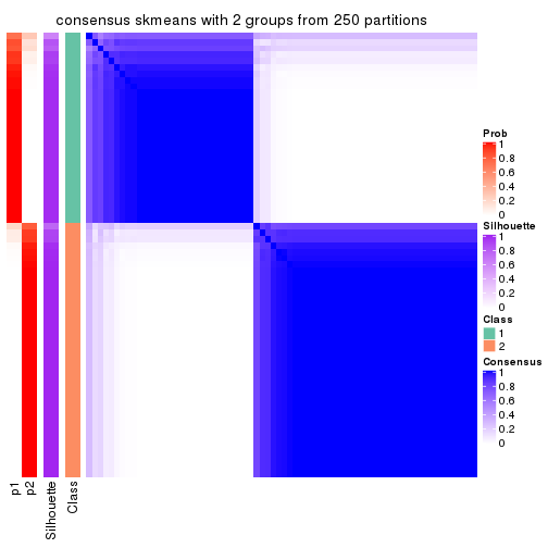
consensus_heatmap(res, k = 3)
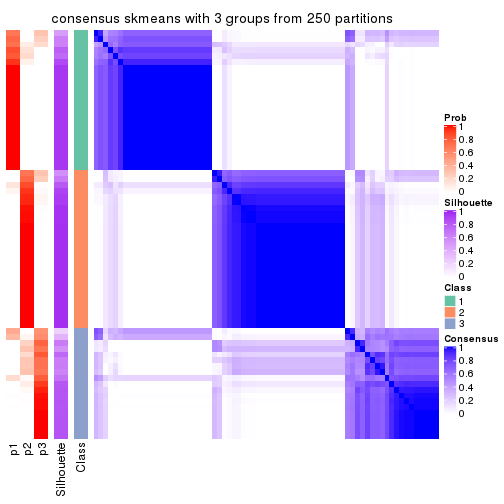
consensus_heatmap(res, k = 4)
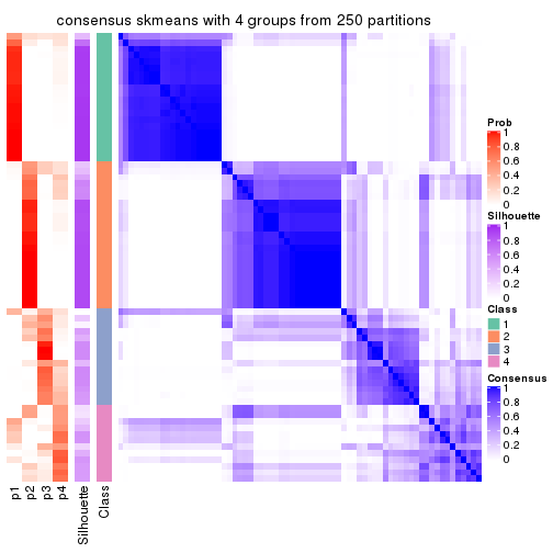
consensus_heatmap(res, k = 5)
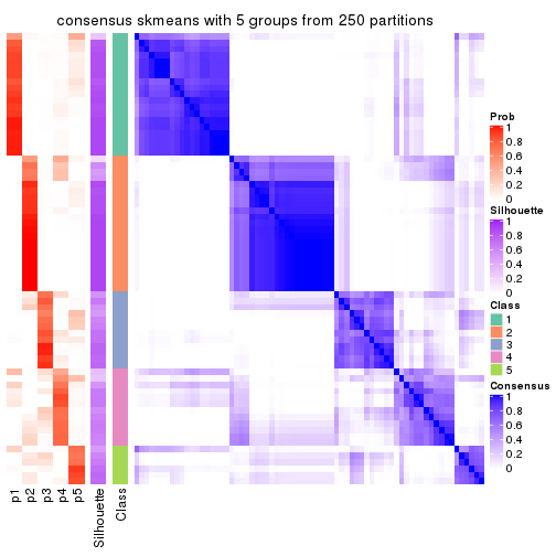
consensus_heatmap(res, k = 6)
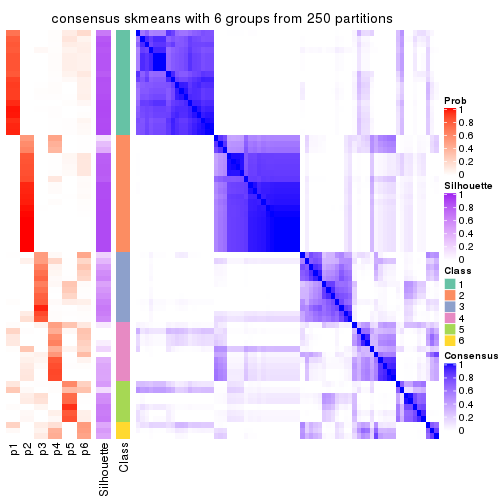
Heatmaps for the membership of samples in all partitions to see how consistent they are:
membership_heatmap(res, k = 2)

membership_heatmap(res, k = 3)
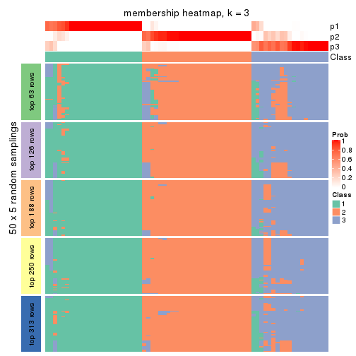
membership_heatmap(res, k = 4)
membership_heatmap(res, k = 5)
membership_heatmap(res, k = 6)
As soon as we have had the classes for columns, we can look for signatures which are significantly different between classes which can be candidate marks for certain classes. Following are the heatmaps for signatures.
Signature heatmaps where rows are scaled:
get_signatures(res, k = 2)
get_signatures(res, k = 3)
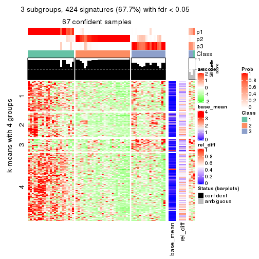
get_signatures(res, k = 4)
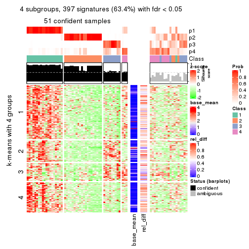
get_signatures(res, k = 5)
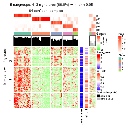
get_signatures(res, k = 6)
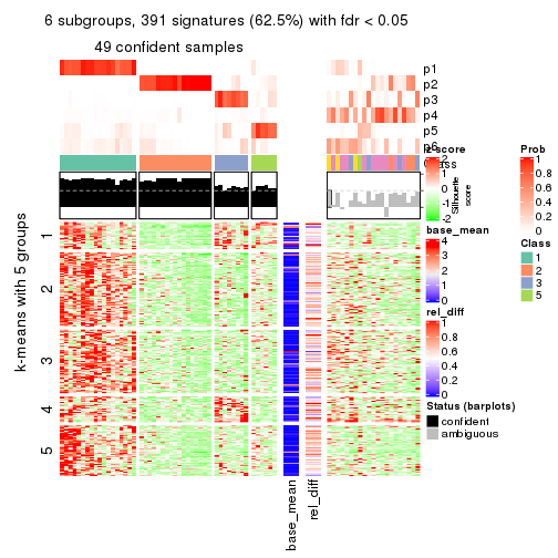
Signature heatmaps where rows are not scaled:
get_signatures(res, k = 2, scale_rows = FALSE)
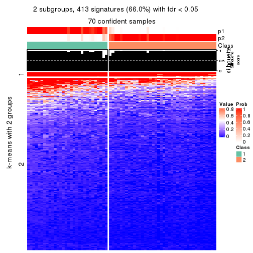
get_signatures(res, k = 3, scale_rows = FALSE)
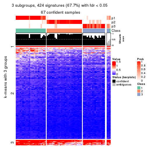
get_signatures(res, k = 4, scale_rows = FALSE)
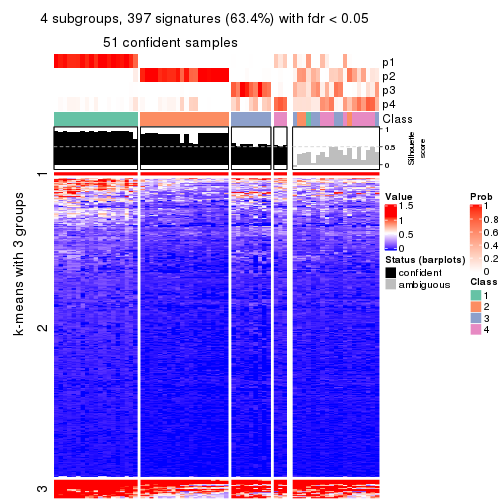
get_signatures(res, k = 5, scale_rows = FALSE)
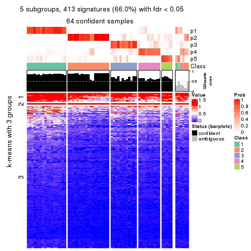
get_signatures(res, k = 6, scale_rows = FALSE)
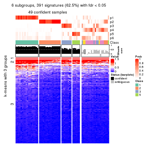
Compare the overlap of signatures from different k:
compare_signatures(res)
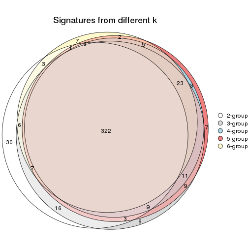
get_signature() returns a data frame invisibly. TO get the list of signatures, the function
call should be assigned to a variable explicitly. In following code, if plot argument is set
to FALSE, no heatmap is plotted while only the differential analysis is performed.
# code only for demonstration
tb = get_signature(res, k = ..., plot = FALSE)
An example of the output of tb is:
#>   which_row         fdr    mean_1    mean_2 scaled_mean_1 scaled_mean_2 km
#> 1        38 0.042760348  8.373488  9.131774    -0.5533452     0.5164555  1
#> 2        40 0.018707592  7.106213  8.469186    -0.6173731     0.5762149  1
#> 3        55 0.019134737 10.221463 11.207825    -0.6159697     0.5749050  1
#> 4        59 0.006059896  5.921854  7.869574    -0.6899429     0.6439467  1
#> 5        60 0.018055526  8.928898 10.211722    -0.6204761     0.5791110  1
#> 6        98 0.009384629 15.714769 14.887706     0.6635654    -0.6193277  2
...
The columns in tb are:
which_row: row indices corresponding to the input matrix.fdr: FDR for the differential test. mean_x: The mean value in group x.scaled_mean_x: The mean value in group x after rows are scaled.km: Row groups if k-means clustering is applied to rows.UMAP plot which shows how samples are separated.
dimension_reduction(res, k = 2, method = "UMAP")
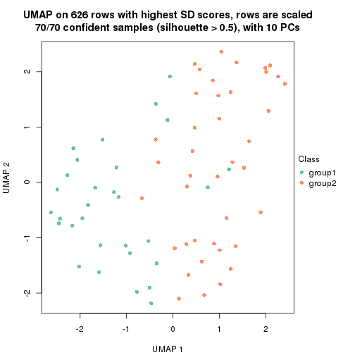
dimension_reduction(res, k = 3, method = "UMAP")
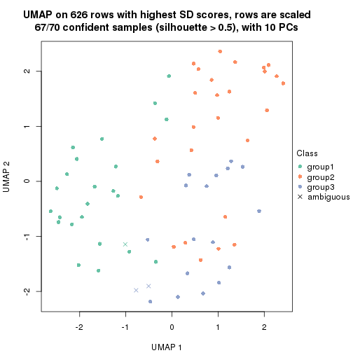
dimension_reduction(res, k = 4, method = "UMAP")
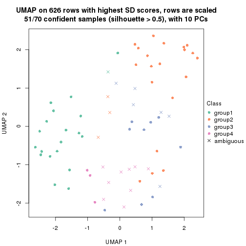
dimension_reduction(res, k = 5, method = "UMAP")
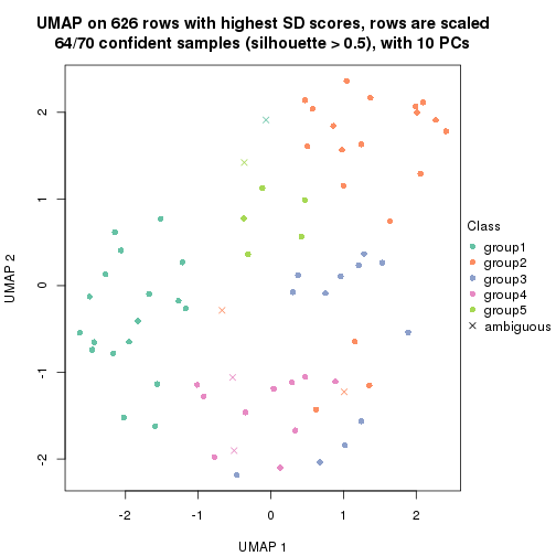
dimension_reduction(res, k = 6, method = "UMAP")
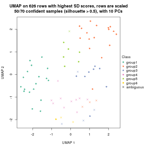
Following heatmap shows how subgroups are split when increasing k:
collect_classes(res)
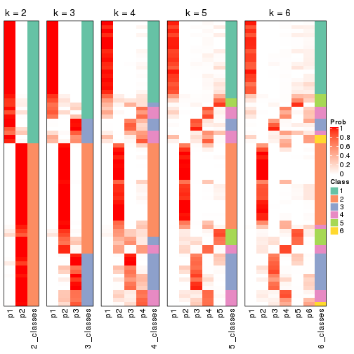
If matrix rows can be associated to genes, consider to use functional_enrichment(res,
...) to perform function enrichment for the signature genes. See this vignette for more detailed explanations.
The object with results only for a single top-value method and a single partition method can be extracted as:
res = res_list["SD", "pam"]
# you can also extract it by
# res = res_list["SD:pam"]
A summary of res and all the functions that can be applied to it:
res
#> A 'ConsensusPartition' object with k = 2, 3, 4, 5, 6.
#>   On a matrix with 626 rows and 70 columns.
#>   Top rows (63, 126, 188, 250, 313) are extracted by 'SD' method.
#>   Subgroups are detected by 'pam' method.
#>   Performed in total 1250 partitions by row resampling.
#>   Best k for subgroups seems to be 2.
#>
#> Following methods can be applied to this 'ConsensusPartition' object:
#>  [1] "cola_report"             "collect_classes"         "collect_plots"
#>  [4] "collect_stats"           "colnames"                "compare_signatures"
#>  [7] "consensus_heatmap"       "dimension_reduction"     "functional_enrichment"
#> [10] "get_anno_col"            "get_anno"                "get_classes"
#> [13] "get_consensus"           "get_matrix"              "get_membership"
#> [16] "get_param"               "get_signatures"          "get_stats"
#> [19] "is_best_k"               "is_stable_k"             "membership_heatmap"
#> [22] "ncol"                    "nrow"                    "plot_ecdf"
#> [25] "rownames"                "select_partition_number" "show"
#> [28] "suggest_best_k"          "test_to_known_factors"
collect_plots() function collects all the plots made from res for all k (number of partitions)
into one single page to provide an easy and fast comparison between different k.
collect_plots(res)
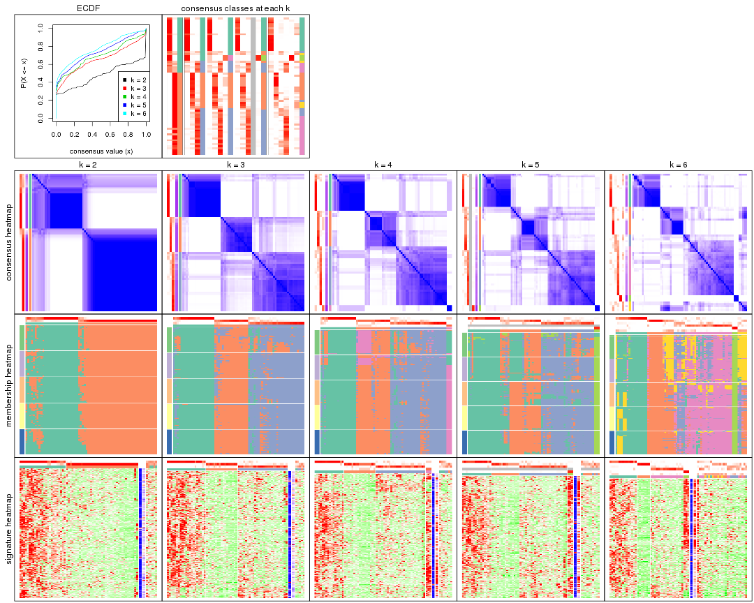
The plots are:
k and the heatmap of
predicted classes for each k.k.k.k.All the plots in panels can be made by individual functions and they are plotted later in this section.
select_partition_number() produces several plots showing different
statistics for choosing “optimized” k. There are following statistics:
k;k, the area increased is defined as \(A_k - A_{k-1}\).The detailed explanations of these statistics can be found in the cola vignette.
Generally speaking, lower PAC score, higher mean silhouette score or higher
concordance corresponds to better partition. Rand index and Jaccard index
measure how similar the current partition is compared to partition with k-1.
If they are too similar, we won't accept k is better than k-1.
select_partition_number(res)
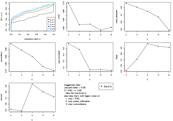
The numeric values for all these statistics can be obtained by get_stats().
get_stats(res)
#>   k 1-PAC mean_silhouette concordance area_increased  Rand Jaccard
#> 2 2 0.718           0.855       0.939         0.4750 0.513   0.513
#> 3 3 0.616           0.803       0.893         0.3828 0.707   0.488
#> 4 4 0.619           0.745       0.851         0.0609 0.976   0.930
#> 5 5 0.590           0.668       0.780         0.0649 0.931   0.802
#> 6 6 0.604           0.489       0.754         0.0505 0.913   0.721
suggest_best_k() suggests the best \(k\) based on these statistics. The rules are as follows:
suggest_best_k(res)
#> [1] 2
Following shows the table of the partitions (You need to click the show/hide
code output link to see it). The membership matrix (columns with name p*)
is inferred by
clue::cl_consensus()
function with the SE method. Basically the value in the membership matrix
represents the probability to belong to a certain group. The finall class
label for an item is determined with the group with highest probability it
belongs to.
In get_classes() function, the entropy is calculated from the membership
matrix and the silhouette score is calculated from the consensus matrix.
cbind(get_classes(res, k = 2), get_membership(res, k = 2))
#>           class entropy silhouette    p1    p2
#> SRR837437     2  0.0000      0.959 0.000 1.000
#> SRR837438     1  0.5294      0.824 0.880 0.120
#> SRR837439     2  0.0000      0.959 0.000 1.000
#> SRR837440     2  0.0000      0.959 0.000 1.000
#> SRR837441     2  0.0000      0.959 0.000 1.000
#> SRR837442     2  0.0000      0.959 0.000 1.000
#> SRR837443     2  0.0000      0.959 0.000 1.000
#> SRR837444     1  0.9909      0.311 0.556 0.444
#> SRR837445     2  0.9661      0.256 0.392 0.608
#> SRR837446     2  0.0000      0.959 0.000 1.000
#> SRR837447     1  0.0000      0.890 1.000 0.000
#> SRR837448     1  0.0000      0.890 1.000 0.000
#> SRR837449     1  0.0000      0.890 1.000 0.000
#> SRR837450     1  0.0000      0.890 1.000 0.000
#> SRR837451     2  0.0000      0.959 0.000 1.000
#> SRR837452     2  0.0000      0.959 0.000 1.000
#> SRR837453     2  0.0000      0.959 0.000 1.000
#> SRR837454     2  0.0000      0.959 0.000 1.000
#> SRR837455     1  0.0000      0.890 1.000 0.000
#> SRR837456     1  0.0000      0.890 1.000 0.000
#> SRR837457     2  0.0000      0.959 0.000 1.000
#> SRR837458     1  0.0000      0.890 1.000 0.000
#> SRR837459     2  0.0000      0.959 0.000 1.000
#> SRR837460     2  0.0000      0.959 0.000 1.000
#> SRR837461     2  0.0000      0.959 0.000 1.000
#> SRR837462     1  0.6438      0.789 0.836 0.164
#> SRR837463     2  0.9998     -0.127 0.492 0.508
#> SRR837464     2  0.0000      0.959 0.000 1.000
#> SRR837465     1  0.9710      0.431 0.600 0.400
#> SRR837466     1  0.0000      0.890 1.000 0.000
#> SRR837467     2  0.0000      0.959 0.000 1.000
#> SRR837468     2  0.9393      0.374 0.356 0.644
#> SRR837469     1  0.0000      0.890 1.000 0.000
#> SRR837470     1  0.0000      0.890 1.000 0.000
#> SRR837471     2  0.0000      0.959 0.000 1.000
#> SRR837472     2  0.0000      0.959 0.000 1.000
#> SRR837473     1  0.4690      0.840 0.900 0.100
#> SRR837474     2  0.0000      0.959 0.000 1.000
#> SRR837475     2  0.0000      0.959 0.000 1.000
#> SRR837476     2  0.0000      0.959 0.000 1.000
#> SRR837477     1  0.7745      0.728 0.772 0.228
#> SRR837478     2  0.0000      0.959 0.000 1.000
#> SRR837479     2  0.0000      0.959 0.000 1.000
#> SRR837480     2  0.0000      0.959 0.000 1.000
#> SRR837481     2  0.1633      0.937 0.024 0.976
#> SRR837482     1  0.9522      0.494 0.628 0.372
#> SRR837483     1  0.0000      0.890 1.000 0.000
#> SRR837484     2  0.0000      0.959 0.000 1.000
#> SRR837485     2  0.0000      0.959 0.000 1.000
#> SRR837486     2  0.4022      0.878 0.080 0.920
#> SRR837487     2  0.0000      0.959 0.000 1.000
#> SRR837488     2  0.0000      0.959 0.000 1.000
#> SRR837489     2  0.0000      0.959 0.000 1.000
#> SRR837490     2  0.0000      0.959 0.000 1.000
#> SRR837491     2  0.5737      0.807 0.136 0.864
#> SRR837492     1  0.9248      0.555 0.660 0.340
#> SRR837493     1  0.9323      0.542 0.652 0.348
#> SRR837494     2  0.0000      0.959 0.000 1.000
#> SRR837495     1  0.8763      0.642 0.704 0.296
#> SRR837496     1  0.0000      0.890 1.000 0.000
#> SRR837497     1  0.0000      0.890 1.000 0.000
#> SRR837498     1  0.0000      0.890 1.000 0.000
#> SRR837499     1  0.0000      0.890 1.000 0.000
#> SRR837500     1  0.0000      0.890 1.000 0.000
#> SRR837501     2  0.0376      0.955 0.004 0.996
#> SRR837502     1  0.0000      0.890 1.000 0.000
#> SRR837503     1  0.0000      0.890 1.000 0.000
#> SRR837504     2  0.0000      0.959 0.000 1.000
#> SRR837505     2  0.0000      0.959 0.000 1.000
#> SRR837506     2  0.0000      0.959 0.000 1.000
cbind(get_classes(res, k = 3), get_membership(res, k = 3))
#>           class entropy silhouette    p1    p2    p3
#> SRR837437     3  0.4654      0.747 0.000 0.208 0.792
#> SRR837438     1  0.5058      0.628 0.756 0.000 0.244
#> SRR837439     3  0.2796      0.826 0.000 0.092 0.908
#> SRR837440     3  0.2066      0.835 0.000 0.060 0.940
#> SRR837441     3  0.2711      0.828 0.000 0.088 0.912
#> SRR837442     3  0.4654      0.758 0.000 0.208 0.792
#> SRR837443     3  0.1860      0.836 0.000 0.052 0.948
#> SRR837444     3  0.3083      0.829 0.060 0.024 0.916
#> SRR837445     3  0.5961      0.779 0.096 0.112 0.792
#> SRR837446     3  0.0237      0.833 0.000 0.004 0.996
#> SRR837447     1  0.0000      0.945 1.000 0.000 0.000
#> SRR837448     1  0.0424      0.941 0.992 0.008 0.000
#> SRR837449     1  0.0000      0.945 1.000 0.000 0.000
#> SRR837450     1  0.0424      0.941 0.992 0.008 0.000
#> SRR837451     2  0.1163      0.888 0.000 0.972 0.028
#> SRR837452     2  0.0892      0.888 0.000 0.980 0.020
#> SRR837453     2  0.0892      0.888 0.000 0.980 0.020
#> SRR837454     2  0.0424      0.884 0.000 0.992 0.008
#> SRR837455     1  0.0000      0.945 1.000 0.000 0.000
#> SRR837456     1  0.0000      0.945 1.000 0.000 0.000
#> SRR837457     2  0.1753      0.882 0.000 0.952 0.048
#> SRR837458     1  0.0000      0.945 1.000 0.000 0.000
#> SRR837459     2  0.1289      0.887 0.000 0.968 0.032
#> SRR837460     2  0.1860      0.881 0.000 0.948 0.052
#> SRR837461     3  0.2448      0.831 0.000 0.076 0.924
#> SRR837462     3  0.5873      0.584 0.312 0.004 0.684
#> SRR837463     3  0.3375      0.835 0.044 0.048 0.908
#> SRR837464     3  0.2066      0.835 0.000 0.060 0.940
#> SRR837465     3  0.7944      0.645 0.212 0.132 0.656
#> SRR837466     1  0.0424      0.941 0.992 0.008 0.000
#> SRR837467     3  0.5397      0.655 0.000 0.280 0.720
#> SRR837468     3  0.0237      0.831 0.004 0.000 0.996
#> SRR837469     1  0.0000      0.945 1.000 0.000 0.000
#> SRR837470     1  0.0000      0.945 1.000 0.000 0.000
#> SRR837471     2  0.2625      0.870 0.000 0.916 0.084
#> SRR837472     2  0.1163      0.888 0.000 0.972 0.028
#> SRR837473     1  0.3826      0.819 0.868 0.124 0.008
#> SRR837474     2  0.4235      0.783 0.000 0.824 0.176
#> SRR837475     2  0.0592      0.885 0.000 0.988 0.012
#> SRR837476     2  0.2448      0.877 0.000 0.924 0.076
#> SRR837477     1  0.8247      0.347 0.580 0.096 0.324
#> SRR837478     2  0.5733      0.558 0.000 0.676 0.324
#> SRR837479     3  0.0237      0.832 0.000 0.004 0.996
#> SRR837480     3  0.5948      0.390 0.000 0.360 0.640
#> SRR837481     3  0.0661      0.832 0.004 0.008 0.988
#> SRR837482     3  0.3879      0.766 0.152 0.000 0.848
#> SRR837483     1  0.0237      0.942 0.996 0.000 0.004
#> SRR837484     3  0.4750      0.692 0.000 0.216 0.784
#> SRR837485     3  0.5678      0.491 0.000 0.316 0.684
#> SRR837486     3  0.1015      0.834 0.012 0.008 0.980
#> SRR837487     2  0.3412      0.856 0.000 0.876 0.124
#> SRR837488     2  0.0592      0.886 0.000 0.988 0.012
#> SRR837489     2  0.6180      0.236 0.000 0.584 0.416
#> SRR837490     2  0.2356      0.878 0.000 0.928 0.072
#> SRR837491     3  0.5618      0.784 0.048 0.156 0.796
#> SRR837492     1  0.7217      0.653 0.716 0.152 0.132
#> SRR837493     3  0.6082      0.623 0.296 0.012 0.692
#> SRR837494     2  0.5760      0.537 0.000 0.672 0.328
#> SRR837495     3  0.8699      0.332 0.376 0.112 0.512
#> SRR837496     1  0.0000      0.945 1.000 0.000 0.000
#> SRR837497     1  0.0000      0.945 1.000 0.000 0.000
#> SRR837498     1  0.0000      0.945 1.000 0.000 0.000
#> SRR837499     1  0.0000      0.945 1.000 0.000 0.000
#> SRR837500     1  0.0000      0.945 1.000 0.000 0.000
#> SRR837501     3  0.0424      0.833 0.000 0.008 0.992
#> SRR837502     1  0.0000      0.945 1.000 0.000 0.000
#> SRR837503     1  0.0000      0.945 1.000 0.000 0.000
#> SRR837504     3  0.1031      0.835 0.000 0.024 0.976
#> SRR837505     3  0.1163      0.834 0.000 0.028 0.972
#> SRR837506     3  0.4235      0.727 0.000 0.176 0.824
cbind(get_classes(res, k = 4), get_membership(res, k = 4))
#>           class entropy silhouette    p1    p2    p3    p4
#> SRR837437     3  0.4086      0.745 0.000 0.216 0.776 0.008
#> SRR837438     1  0.4262      0.471 0.756 0.008 0.236 0.000
#> SRR837439     3  0.2530      0.816 0.000 0.112 0.888 0.000
#> SRR837440     3  0.1637      0.829 0.000 0.060 0.940 0.000
#> SRR837441     3  0.2345      0.820 0.000 0.100 0.900 0.000
#> SRR837442     3  0.4454      0.678 0.000 0.308 0.692 0.000
#> SRR837443     3  0.1389      0.829 0.000 0.048 0.952 0.000
#> SRR837444     3  0.2596      0.816 0.068 0.024 0.908 0.000
#> SRR837445     3  0.4916      0.765 0.056 0.184 0.760 0.000
#> SRR837446     3  0.0524      0.825 0.000 0.004 0.988 0.008
#> SRR837447     1  0.0469      0.853 0.988 0.000 0.000 0.012
#> SRR837448     4  0.4164      1.000 0.264 0.000 0.000 0.736
#> SRR837449     1  0.0188      0.860 0.996 0.000 0.000 0.004
#> SRR837450     4  0.4164      1.000 0.264 0.000 0.000 0.736
#> SRR837451     2  0.4546      0.765 0.000 0.732 0.012 0.256
#> SRR837452     2  0.0524      0.784 0.000 0.988 0.008 0.004
#> SRR837453     2  0.4422      0.766 0.000 0.736 0.008 0.256
#> SRR837454     2  0.4103      0.765 0.000 0.744 0.000 0.256
#> SRR837455     1  0.0188      0.860 0.996 0.000 0.000 0.004
#> SRR837456     1  0.0188      0.860 0.996 0.000 0.000 0.004
#> SRR837457     2  0.4546      0.765 0.000 0.732 0.012 0.256
#> SRR837458     1  0.0188      0.860 0.996 0.000 0.000 0.004
#> SRR837459     2  0.4422      0.766 0.000 0.736 0.008 0.256
#> SRR837460     2  0.4546      0.765 0.000 0.732 0.012 0.256
#> SRR837461     3  0.2670      0.826 0.000 0.040 0.908 0.052
#> SRR837462     3  0.4454      0.564 0.308 0.000 0.692 0.000
#> SRR837463     3  0.2919      0.821 0.060 0.044 0.896 0.000
#> SRR837464     3  0.1716      0.828 0.000 0.064 0.936 0.000
#> SRR837465     3  0.6840      0.582 0.220 0.180 0.600 0.000
#> SRR837466     4  0.4164      1.000 0.264 0.000 0.000 0.736
#> SRR837467     3  0.4560      0.677 0.000 0.296 0.700 0.004
#> SRR837468     3  0.0336      0.823 0.000 0.000 0.992 0.008
#> SRR837469     1  0.0000      0.861 1.000 0.000 0.000 0.000
#> SRR837470     1  0.0000      0.861 1.000 0.000 0.000 0.000
#> SRR837471     2  0.1022      0.777 0.000 0.968 0.032 0.000
#> SRR837472     2  0.0469      0.781 0.000 0.988 0.012 0.000
#> SRR837473     1  0.4343      0.508 0.732 0.264 0.004 0.000
#> SRR837474     2  0.2081      0.745 0.000 0.916 0.084 0.000
#> SRR837475     2  0.0336      0.784 0.000 0.992 0.000 0.008
#> SRR837476     2  0.0707      0.781 0.000 0.980 0.020 0.000
#> SRR837477     1  0.7900      0.110 0.456 0.224 0.312 0.008
#> SRR837478     2  0.4964      0.563 0.000 0.716 0.256 0.028
#> SRR837479     3  0.0524      0.824 0.000 0.004 0.988 0.008
#> SRR837480     3  0.5183      0.317 0.000 0.408 0.584 0.008
#> SRR837481     3  0.0524      0.824 0.000 0.004 0.988 0.008
#> SRR837482     3  0.3401      0.749 0.152 0.000 0.840 0.008
#> SRR837483     1  0.0188      0.857 0.996 0.000 0.004 0.000
#> SRR837484     3  0.3668      0.705 0.000 0.188 0.808 0.004
#> SRR837485     3  0.4454      0.498 0.000 0.308 0.692 0.000
#> SRR837486     3  0.0188      0.825 0.004 0.000 0.996 0.000
#> SRR837487     2  0.1792      0.782 0.000 0.932 0.068 0.000
#> SRR837488     2  0.4422      0.766 0.000 0.736 0.008 0.256
#> SRR837489     2  0.4477      0.335 0.000 0.688 0.312 0.000
#> SRR837490     2  0.2840      0.788 0.000 0.900 0.056 0.044
#> SRR837491     3  0.4994      0.751 0.048 0.208 0.744 0.000
#> SRR837492     1  0.6770      0.309 0.580 0.292 0.128 0.000
#> SRR837493     3  0.4632      0.577 0.308 0.004 0.688 0.000
#> SRR837494     2  0.6746      0.505 0.000 0.568 0.316 0.116
#> SRR837495     3  0.7536      0.394 0.264 0.244 0.492 0.000
#> SRR837496     1  0.0000      0.861 1.000 0.000 0.000 0.000
#> SRR837497     1  0.0000      0.861 1.000 0.000 0.000 0.000
#> SRR837498     1  0.0000      0.861 1.000 0.000 0.000 0.000
#> SRR837499     1  0.0000      0.861 1.000 0.000 0.000 0.000
#> SRR837500     1  0.0000      0.861 1.000 0.000 0.000 0.000
#> SRR837501     3  0.0000      0.824 0.000 0.000 1.000 0.000
#> SRR837502     1  0.0000      0.861 1.000 0.000 0.000 0.000
#> SRR837503     1  0.0000      0.861 1.000 0.000 0.000 0.000
#> SRR837504     3  0.0524      0.826 0.000 0.008 0.988 0.004
#> SRR837505     3  0.1489      0.819 0.000 0.004 0.952 0.044
#> SRR837506     3  0.4452      0.710 0.000 0.156 0.796 0.048
cbind(get_classes(res, k = 5), get_membership(res, k = 5))
#>           class entropy silhouette    p1    p2    p3 p4    p5
#> SRR837437     3  0.4083    0.70310 0.000 0.228 0.744 NA 0.000
#> SRR837438     1  0.3849    0.58884 0.752 0.016 0.232 NA 0.000
#> SRR837439     3  0.2629    0.77617 0.000 0.136 0.860 NA 0.000
#> SRR837440     3  0.2325    0.79959 0.000 0.068 0.904 NA 0.000
#> SRR837441     3  0.2280    0.78276 0.000 0.120 0.880 NA 0.000
#> SRR837442     3  0.4219    0.48498 0.000 0.416 0.584 NA 0.000
#> SRR837443     3  0.1571    0.79797 0.000 0.060 0.936 NA 0.004
#> SRR837444     3  0.2767    0.78841 0.088 0.020 0.884 NA 0.004
#> SRR837445     3  0.5080    0.67640 0.052 0.248 0.688 NA 0.004
#> SRR837446     3  0.1483    0.79714 0.000 0.008 0.952 NA 0.028
#> SRR837447     1  0.2011    0.84397 0.908 0.000 0.000 NA 0.088
#> SRR837448     5  0.1043    0.99462 0.040 0.000 0.000 NA 0.960
#> SRR837449     1  0.0404    0.88747 0.988 0.000 0.000 NA 0.012
#> SRR837450     5  0.1043    0.99462 0.040 0.000 0.000 NA 0.960
#> SRR837451     2  0.4434    0.54527 0.000 0.536 0.004 NA 0.000
#> SRR837452     2  0.2439    0.60674 0.000 0.876 0.004 NA 0.000
#> SRR837453     2  0.4434    0.54527 0.000 0.536 0.004 NA 0.000
#> SRR837454     2  0.4287    0.54520 0.000 0.540 0.000 NA 0.000
#> SRR837455     1  0.2727    0.82710 0.868 0.000 0.000 NA 0.016
#> SRR837456     1  0.2727    0.82710 0.868 0.000 0.000 NA 0.016
#> SRR837457     2  0.4434    0.54527 0.000 0.536 0.004 NA 0.000
#> SRR837458     1  0.3877    0.74999 0.764 0.000 0.000 NA 0.024
#> SRR837459     2  0.4434    0.54527 0.000 0.536 0.004 NA 0.000
#> SRR837460     2  0.4434    0.54527 0.000 0.536 0.004 NA 0.000
#> SRR837461     3  0.2661    0.79647 0.000 0.056 0.888 NA 0.000
#> SRR837462     3  0.4910    0.61263 0.288 0.012 0.672 NA 0.004
#> SRR837463     3  0.2450    0.79813 0.052 0.048 0.900 NA 0.000
#> SRR837464     3  0.2046    0.79837 0.000 0.068 0.916 NA 0.000
#> SRR837465     3  0.6388    0.45408 0.244 0.240 0.516 NA 0.000
#> SRR837466     5  0.1197    0.98923 0.048 0.000 0.000 NA 0.952
#> SRR837467     3  0.4924    0.62238 0.000 0.272 0.668 NA 0.000
#> SRR837468     3  0.2685    0.78487 0.000 0.000 0.880 NA 0.028
#> SRR837469     1  0.2304    0.84094 0.892 0.000 0.000 NA 0.008
#> SRR837470     1  0.2416    0.83871 0.888 0.000 0.000 NA 0.012
#> SRR837471     2  0.0898    0.59096 0.000 0.972 0.020 NA 0.000
#> SRR837472     2  0.0798    0.59800 0.000 0.976 0.008 NA 0.000
#> SRR837473     1  0.4367    0.33256 0.580 0.416 0.000 NA 0.000
#> SRR837474     2  0.1914    0.58118 0.000 0.924 0.060 NA 0.000
#> SRR837475     2  0.1197    0.60242 0.000 0.952 0.000 NA 0.000
#> SRR837476     2  0.1012    0.59752 0.000 0.968 0.020 NA 0.000
#> SRR837477     2  0.8752    0.10587 0.200 0.372 0.144 NA 0.024
#> SRR837478     2  0.6512    0.37337 0.000 0.540 0.128 NA 0.024
#> SRR837479     3  0.4570    0.66466 0.000 0.008 0.720 NA 0.036
#> SRR837480     2  0.7436   -0.02786 0.000 0.352 0.352 NA 0.032
#> SRR837481     3  0.3195    0.77095 0.000 0.004 0.856 NA 0.040
#> SRR837482     3  0.4026    0.75280 0.140 0.004 0.808 NA 0.020
#> SRR837483     1  0.0162    0.88941 0.996 0.000 0.004 NA 0.000
#> SRR837484     3  0.5056    0.67808 0.000 0.160 0.732 NA 0.020
#> SRR837485     3  0.5840    0.53618 0.000 0.228 0.652 NA 0.032
#> SRR837486     3  0.3018    0.78058 0.000 0.008 0.872 NA 0.036
#> SRR837487     2  0.3934    0.59049 0.000 0.820 0.060 NA 0.016
#> SRR837488     2  0.4430    0.54620 0.000 0.540 0.004 NA 0.000
#> SRR837489     2  0.3353    0.46059 0.000 0.796 0.196 NA 0.000
#> SRR837490     2  0.4395    0.59619 0.000 0.748 0.064 NA 0.000
#> SRR837491     3  0.4974    0.63140 0.048 0.288 0.660 NA 0.000
#> SRR837492     2  0.7518    0.13265 0.256 0.452 0.056 NA 0.000
#> SRR837493     3  0.4232    0.58983 0.312 0.012 0.676 NA 0.000
#> SRR837494     2  0.6486    0.39198 0.000 0.480 0.308 NA 0.000
#> SRR837495     2  0.8387    0.00336 0.184 0.376 0.276 NA 0.004
#> SRR837496     1  0.0162    0.88980 0.996 0.000 0.000 NA 0.000
#> SRR837497     1  0.0000    0.89073 1.000 0.000 0.000 NA 0.000
#> SRR837498     1  0.0000    0.89073 1.000 0.000 0.000 NA 0.000
#> SRR837499     1  0.0000    0.89073 1.000 0.000 0.000 NA 0.000
#> SRR837500     1  0.0000    0.89073 1.000 0.000 0.000 NA 0.000
#> SRR837501     3  0.0955    0.79269 0.000 0.000 0.968 NA 0.004
#> SRR837502     1  0.0000    0.89073 1.000 0.000 0.000 NA 0.000
#> SRR837503     1  0.0000    0.89073 1.000 0.000 0.000 NA 0.000
#> SRR837504     3  0.1442    0.79504 0.000 0.012 0.952 NA 0.004
#> SRR837505     3  0.2573    0.78162 0.000 0.000 0.880 NA 0.016
#> SRR837506     3  0.5553    0.63200 0.000 0.104 0.688 NA 0.024
cbind(get_classes(res, k = 6), get_membership(res, k = 6))
#>           class entropy silhouette    p1    p2    p3    p4    p5    p6
#> SRR837437     4  0.3307   0.588620 0.000 0.108 0.000 0.820 0.000 0.072
#> SRR837438     1  0.3508   0.502954 0.704 0.000 0.000 0.292 0.000 0.004
#> SRR837439     4  0.1075   0.679615 0.000 0.000 0.000 0.952 0.000 0.048
#> SRR837440     4  0.1918   0.678740 0.000 0.000 0.088 0.904 0.000 0.008
#> SRR837441     4  0.0937   0.681552 0.000 0.000 0.000 0.960 0.000 0.040
#> SRR837442     4  0.4121   0.297448 0.000 0.016 0.000 0.604 0.000 0.380
#> SRR837443     4  0.0291   0.684696 0.000 0.000 0.004 0.992 0.000 0.004
#> SRR837444     4  0.2365   0.676259 0.068 0.000 0.024 0.896 0.000 0.012
#> SRR837445     4  0.4242   0.513043 0.040 0.000 0.012 0.716 0.000 0.232
#> SRR837446     4  0.2558   0.647562 0.000 0.000 0.156 0.840 0.000 0.004
#> SRR837447     1  0.2741   0.771642 0.868 0.000 0.032 0.000 0.092 0.008
#> SRR837448     5  0.0000   0.993712 0.000 0.000 0.000 0.000 1.000 0.000
#> SRR837449     1  0.0653   0.825327 0.980 0.000 0.012 0.000 0.004 0.004
#> SRR837450     5  0.0000   0.993712 0.000 0.000 0.000 0.000 1.000 0.000
#> SRR837451     2  0.0000   0.657513 0.000 1.000 0.000 0.000 0.000 0.000
#> SRR837452     2  0.3830   0.187216 0.000 0.620 0.004 0.000 0.000 0.376
#> SRR837453     2  0.0000   0.657513 0.000 1.000 0.000 0.000 0.000 0.000
#> SRR837454     2  0.0000   0.657513 0.000 1.000 0.000 0.000 0.000 0.000
#> SRR837455     1  0.4440   0.666614 0.716 0.000 0.076 0.000 0.008 0.200
#> SRR837456     1  0.4440   0.666614 0.716 0.000 0.076 0.000 0.008 0.200
#> SRR837457     2  0.0000   0.657513 0.000 1.000 0.000 0.000 0.000 0.000
#> SRR837458     1  0.5775   0.440485 0.484 0.000 0.116 0.000 0.016 0.384
#> SRR837459     2  0.0000   0.657513 0.000 1.000 0.000 0.000 0.000 0.000
#> SRR837460     2  0.0000   0.657513 0.000 1.000 0.000 0.000 0.000 0.000
#> SRR837461     4  0.1036   0.687496 0.000 0.004 0.024 0.964 0.000 0.008
#> SRR837462     4  0.5071   0.423204 0.276 0.000 0.084 0.628 0.000 0.012
#> SRR837463     4  0.1148   0.686681 0.020 0.000 0.016 0.960 0.000 0.004
#> SRR837464     4  0.1584   0.684339 0.000 0.000 0.064 0.928 0.000 0.008
#> SRR837465     4  0.5549   0.261112 0.232 0.000 0.000 0.556 0.000 0.212
#> SRR837466     5  0.0260   0.987401 0.008 0.000 0.000 0.000 0.992 0.000
#> SRR837467     4  0.3782   0.547677 0.000 0.124 0.000 0.780 0.000 0.096
#> SRR837468     4  0.4674   0.543582 0.000 0.000 0.236 0.680 0.008 0.076
#> SRR837469     1  0.4257   0.664596 0.724 0.000 0.056 0.000 0.008 0.212
#> SRR837470     1  0.4409   0.659238 0.716 0.000 0.060 0.000 0.012 0.212
#> SRR837471     6  0.4534   0.010032 0.000 0.472 0.000 0.032 0.000 0.496
#> SRR837472     2  0.4336  -0.163171 0.000 0.504 0.000 0.020 0.000 0.476
#> SRR837473     1  0.3966   0.128889 0.552 0.000 0.000 0.004 0.000 0.444
#> SRR837474     6  0.4897   0.104138 0.000 0.448 0.000 0.060 0.000 0.492
#> SRR837475     2  0.3979  -0.062155 0.000 0.540 0.000 0.004 0.000 0.456
#> SRR837476     2  0.4532  -0.173717 0.000 0.500 0.000 0.032 0.000 0.468
#> SRR837477     3  0.6182  -0.000401 0.084 0.004 0.460 0.052 0.000 0.400
#> SRR837478     3  0.6246  -0.005611 0.000 0.144 0.476 0.036 0.000 0.344
#> SRR837479     3  0.4957   0.140061 0.000 0.000 0.520 0.412 0.000 0.068
#> SRR837480     3  0.6582   0.271263 0.000 0.080 0.520 0.164 0.000 0.236
#> SRR837481     4  0.4262   0.149257 0.000 0.000 0.476 0.508 0.000 0.016
#> SRR837482     4  0.4467   0.556505 0.092 0.000 0.192 0.712 0.000 0.004
#> SRR837483     1  0.0260   0.828528 0.992 0.000 0.008 0.000 0.000 0.000
#> SRR837484     4  0.6040   0.124430 0.000 0.140 0.348 0.488 0.000 0.024
#> SRR837485     3  0.6538  -0.048614 0.000 0.192 0.388 0.384 0.000 0.036
#> SRR837486     4  0.4116   0.356973 0.000 0.000 0.416 0.572 0.000 0.012
#> SRR837487     2  0.6213   0.167532 0.000 0.508 0.240 0.024 0.000 0.228
#> SRR837488     2  0.0291   0.654030 0.000 0.992 0.000 0.004 0.000 0.004
#> SRR837489     6  0.5767   0.312972 0.000 0.300 0.000 0.204 0.000 0.496
#> SRR837490     2  0.4265   0.452534 0.000 0.728 0.000 0.100 0.000 0.172
#> SRR837491     4  0.3798   0.532549 0.032 0.004 0.000 0.748 0.000 0.216
#> SRR837492     6  0.5870   0.047736 0.112 0.008 0.332 0.016 0.000 0.532
#> SRR837493     4  0.3426   0.470870 0.276 0.000 0.000 0.720 0.000 0.004
#> SRR837494     2  0.3945   0.212108 0.000 0.612 0.000 0.380 0.000 0.008
#> SRR837495     6  0.7091  -0.047553 0.112 0.000 0.232 0.208 0.000 0.448
#> SRR837496     1  0.0260   0.828686 0.992 0.000 0.008 0.000 0.000 0.000
#> SRR837497     1  0.0000   0.829995 1.000 0.000 0.000 0.000 0.000 0.000
#> SRR837498     1  0.0146   0.829216 0.996 0.000 0.000 0.000 0.000 0.004
#> SRR837499     1  0.0000   0.829995 1.000 0.000 0.000 0.000 0.000 0.000
#> SRR837500     1  0.0000   0.829995 1.000 0.000 0.000 0.000 0.000 0.000
#> SRR837501     4  0.2520   0.660086 0.000 0.000 0.152 0.844 0.000 0.004
#> SRR837502     1  0.0000   0.829995 1.000 0.000 0.000 0.000 0.000 0.000
#> SRR837503     1  0.0000   0.829995 1.000 0.000 0.000 0.000 0.000 0.000
#> SRR837504     4  0.2706   0.656716 0.000 0.000 0.160 0.832 0.000 0.008
#> SRR837505     4  0.4002   0.565963 0.000 0.036 0.260 0.704 0.000 0.000
#> SRR837506     3  0.5844  -0.042890 0.000 0.096 0.508 0.364 0.000 0.032
Heatmaps for the consensus matrix. It visualizes the probability of two samples to be in a same group.
consensus_heatmap(res, k = 2)
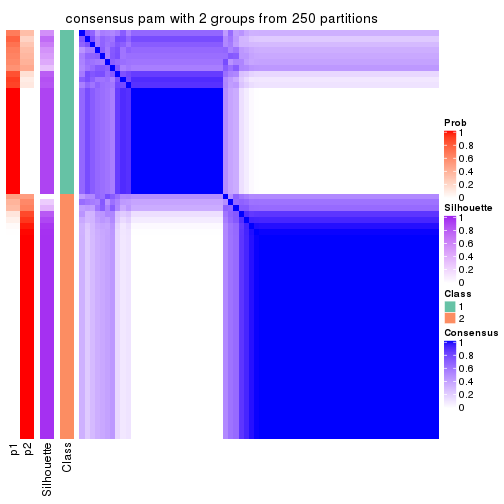
consensus_heatmap(res, k = 3)
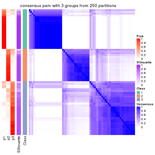
consensus_heatmap(res, k = 4)
consensus_heatmap(res, k = 5)
consensus_heatmap(res, k = 6)
Heatmaps for the membership of samples in all partitions to see how consistent they are:
membership_heatmap(res, k = 2)
membership_heatmap(res, k = 3)
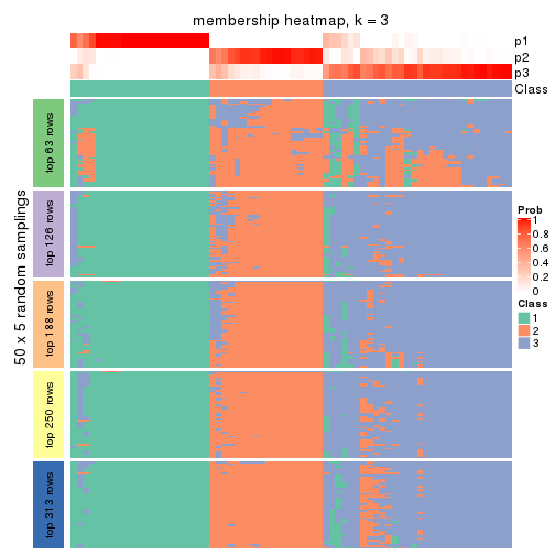
membership_heatmap(res, k = 4)
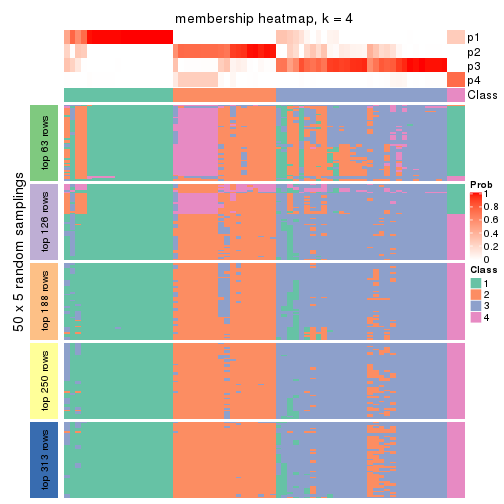
membership_heatmap(res, k = 5)
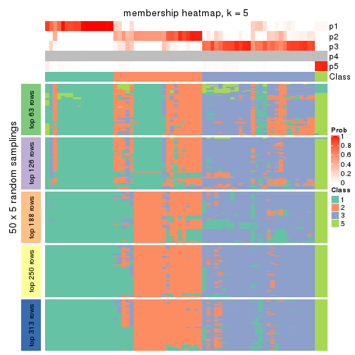
membership_heatmap(res, k = 6)
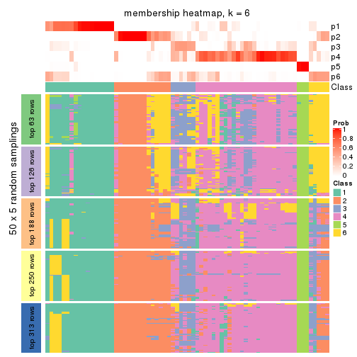
As soon as we have had the classes for columns, we can look for signatures which are significantly different between classes which can be candidate marks for certain classes. Following are the heatmaps for signatures.
Signature heatmaps where rows are scaled:
get_signatures(res, k = 2)
get_signatures(res, k = 3)
get_signatures(res, k = 4)
get_signatures(res, k = 5)
get_signatures(res, k = 6)
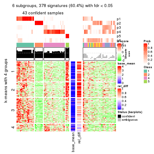
Signature heatmaps where rows are not scaled:
get_signatures(res, k = 2, scale_rows = FALSE)
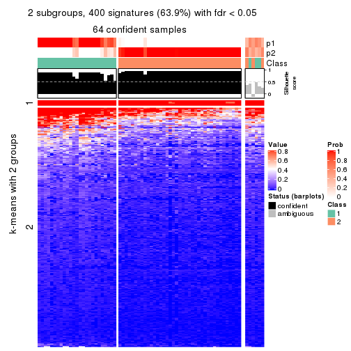
get_signatures(res, k = 3, scale_rows = FALSE)
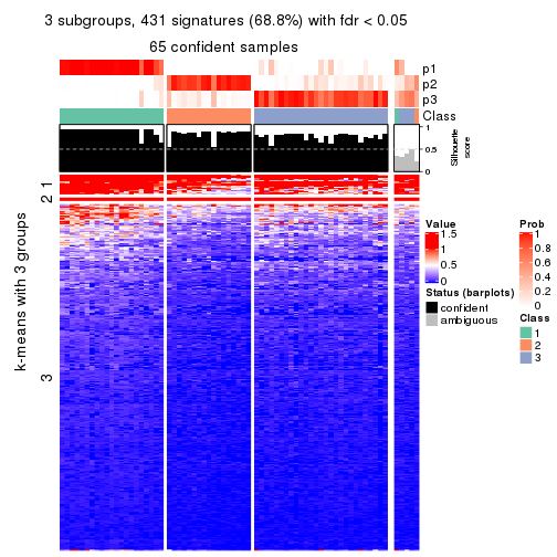
get_signatures(res, k = 4, scale_rows = FALSE)
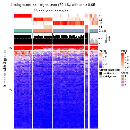
get_signatures(res, k = 5, scale_rows = FALSE)
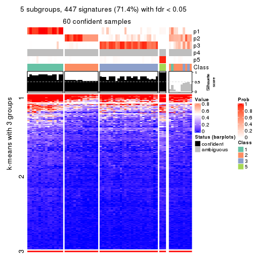
get_signatures(res, k = 6, scale_rows = FALSE)
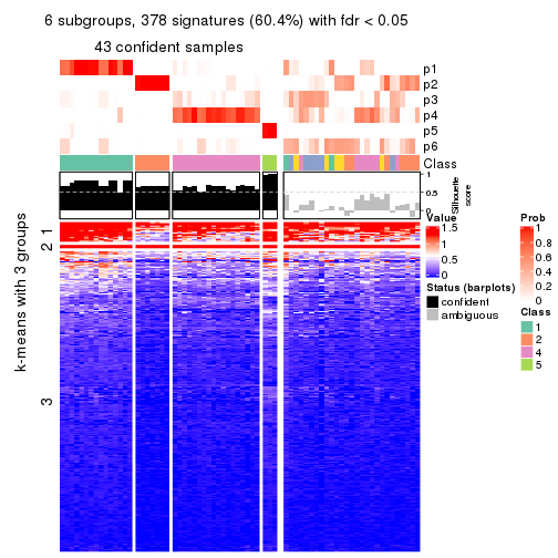
Compare the overlap of signatures from different k:
compare_signatures(res)
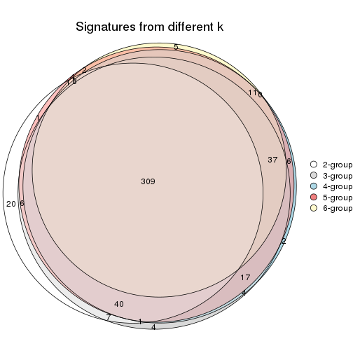
get_signature() returns a data frame invisibly. TO get the list of signatures, the function
call should be assigned to a variable explicitly. In following code, if plot argument is set
to FALSE, no heatmap is plotted while only the differential analysis is performed.
# code only for demonstration
tb = get_signature(res, k = ..., plot = FALSE)
An example of the output of tb is:
#>   which_row         fdr    mean_1    mean_2 scaled_mean_1 scaled_mean_2 km
#> 1        38 0.042760348  8.373488  9.131774    -0.5533452     0.5164555  1
#> 2        40 0.018707592  7.106213  8.469186    -0.6173731     0.5762149  1
#> 3        55 0.019134737 10.221463 11.207825    -0.6159697     0.5749050  1
#> 4        59 0.006059896  5.921854  7.869574    -0.6899429     0.6439467  1
#> 5        60 0.018055526  8.928898 10.211722    -0.6204761     0.5791110  1
#> 6        98 0.009384629 15.714769 14.887706     0.6635654    -0.6193277  2
...
The columns in tb are:
which_row: row indices corresponding to the input matrix.fdr: FDR for the differential test. mean_x: The mean value in group x.scaled_mean_x: The mean value in group x after rows are scaled.km: Row groups if k-means clustering is applied to rows.UMAP plot which shows how samples are separated.
dimension_reduction(res, k = 2, method = "UMAP")
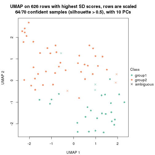
dimension_reduction(res, k = 3, method = "UMAP")

dimension_reduction(res, k = 4, method = "UMAP")
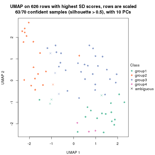
dimension_reduction(res, k = 5, method = "UMAP")
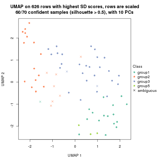
dimension_reduction(res, k = 6, method = "UMAP")
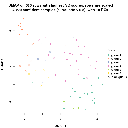
Following heatmap shows how subgroups are split when increasing k:
collect_classes(res)
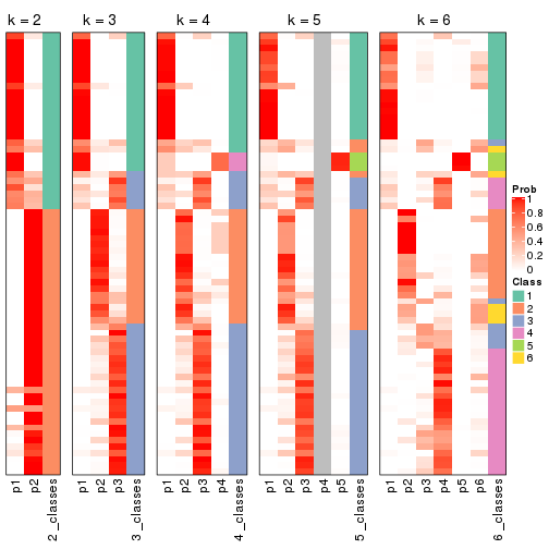
If matrix rows can be associated to genes, consider to use functional_enrichment(res,
...) to perform function enrichment for the signature genes. See this vignette for more detailed explanations.
The object with results only for a single top-value method and a single partition method can be extracted as:
res = res_list["SD", "mclust"]
# you can also extract it by
# res = res_list["SD:mclust"]
A summary of res and all the functions that can be applied to it:
res
#> A 'ConsensusPartition' object with k = 2, 3, 4, 5, 6.
#>   On a matrix with 626 rows and 70 columns.
#>   Top rows (63, 126, 188, 250, 313) are extracted by 'SD' method.
#>   Subgroups are detected by 'mclust' method.
#>   Performed in total 1250 partitions by row resampling.
#>   Best k for subgroups seems to be 2.
#>
#> Following methods can be applied to this 'ConsensusPartition' object:
#>  [1] "cola_report"             "collect_classes"         "collect_plots"
#>  [4] "collect_stats"           "colnames"                "compare_signatures"
#>  [7] "consensus_heatmap"       "dimension_reduction"     "functional_enrichment"
#> [10] "get_anno_col"            "get_anno"                "get_classes"
#> [13] "get_consensus"           "get_matrix"              "get_membership"
#> [16] "get_param"               "get_signatures"          "get_stats"
#> [19] "is_best_k"               "is_stable_k"             "membership_heatmap"
#> [22] "ncol"                    "nrow"                    "plot_ecdf"
#> [25] "rownames"                "select_partition_number" "show"
#> [28] "suggest_best_k"          "test_to_known_factors"
collect_plots() function collects all the plots made from res for all k (number of partitions)
into one single page to provide an easy and fast comparison between different k.
collect_plots(res)
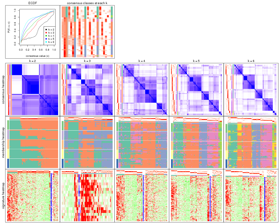
The plots are:
k and the heatmap of
predicted classes for each k.k.k.k.All the plots in panels can be made by individual functions and they are plotted later in this section.
select_partition_number() produces several plots showing different
statistics for choosing “optimized” k. There are following statistics:
k;k, the area increased is defined as \(A_k - A_{k-1}\).The detailed explanations of these statistics can be found in the cola vignette.
Generally speaking, lower PAC score, higher mean silhouette score or higher
concordance corresponds to better partition. Rand index and Jaccard index
measure how similar the current partition is compared to partition with k-1.
If they are too similar, we won't accept k is better than k-1.
select_partition_number(res)
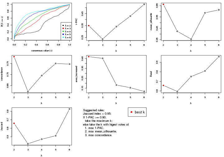
The numeric values for all these statistics can be obtained by get_stats().
get_stats(res)
#>   k 1-PAC mean_silhouette concordance area_increased  Rand Jaccard
#> 2 2 0.350           0.661       0.781         0.4179 0.658   0.658
#> 3 3 0.237           0.424       0.623         0.4013 0.595   0.418
#> 4 4 0.341           0.355       0.696         0.1321 0.751   0.472
#> 5 5 0.429           0.587       0.750         0.1047 0.810   0.512
#> 6 6 0.527           0.613       0.747         0.0672 0.959   0.826
suggest_best_k() suggests the best \(k\) based on these statistics. The rules are as follows:
suggest_best_k(res)
#> [1] 2
Following shows the table of the partitions (You need to click the show/hide
code output link to see it). The membership matrix (columns with name p*)
is inferred by
clue::cl_consensus()
function with the SE method. Basically the value in the membership matrix
represents the probability to belong to a certain group. The finall class
label for an item is determined with the group with highest probability it
belongs to.
In get_classes() function, the entropy is calculated from the membership
matrix and the silhouette score is calculated from the consensus matrix.
cbind(get_classes(res, k = 2), get_membership(res, k = 2))
#>           class entropy silhouette    p1    p2
#> SRR837437     2  0.9983      0.667 0.476 0.524
#> SRR837438     2  0.4815      0.575 0.104 0.896
#> SRR837439     2  0.6623      0.647 0.172 0.828
#> SRR837440     2  0.8861      0.676 0.304 0.696
#> SRR837441     2  0.8813      0.672 0.300 0.700
#> SRR837442     2  0.9993      0.665 0.484 0.516
#> SRR837443     2  0.9000      0.673 0.316 0.684
#> SRR837444     2  0.4562      0.615 0.096 0.904
#> SRR837445     2  0.9686      0.673 0.396 0.604
#> SRR837446     2  0.2423      0.580 0.040 0.960
#> SRR837447     1  0.9998      0.998 0.508 0.492
#> SRR837448     1  0.9998      0.998 0.508 0.492
#> SRR837449     1  0.9993      0.988 0.516 0.484
#> SRR837450     1  0.9998      0.998 0.508 0.492
#> SRR837451     2  0.9998      0.663 0.492 0.508
#> SRR837452     2  0.9815      0.670 0.420 0.580
#> SRR837453     2  0.9998      0.663 0.492 0.508
#> SRR837454     2  0.9998      0.663 0.492 0.508
#> SRR837455     1  0.9998      0.998 0.508 0.492
#> SRR837456     1  0.9998      0.998 0.508 0.492
#> SRR837457     2  0.9998      0.663 0.492 0.508
#> SRR837458     1  0.9998      0.998 0.508 0.492
#> SRR837459     2  0.9998      0.663 0.492 0.508
#> SRR837460     2  0.9998      0.663 0.492 0.508
#> SRR837461     2  0.8499      0.671 0.276 0.724
#> SRR837462     2  0.1843      0.497 0.028 0.972
#> SRR837463     2  0.5059      0.512 0.112 0.888
#> SRR837464     2  0.3879      0.600 0.076 0.924
#> SRR837465     2  0.4815      0.620 0.104 0.896
#> SRR837466     1  0.9998      0.998 0.508 0.492
#> SRR837467     2  0.9988      0.666 0.480 0.520
#> SRR837468     2  0.3274      0.430 0.060 0.940
#> SRR837469     1  0.9998      0.998 0.508 0.492
#> SRR837470     1  0.9998      0.998 0.508 0.492
#> SRR837471     2  0.9998      0.663 0.492 0.508
#> SRR837472     2  0.9998      0.663 0.492 0.508
#> SRR837473     2  0.6343      0.633 0.160 0.840
#> SRR837474     2  0.9998      0.663 0.492 0.508
#> SRR837475     2  0.9970      0.668 0.468 0.532
#> SRR837476     2  0.9998      0.663 0.492 0.508
#> SRR837477     2  0.2236      0.482 0.036 0.964
#> SRR837478     2  0.0672      0.550 0.008 0.992
#> SRR837479     2  0.0000      0.541 0.000 1.000
#> SRR837480     2  0.0938      0.555 0.012 0.988
#> SRR837481     2  0.0000      0.541 0.000 1.000
#> SRR837482     2  0.2948      0.449 0.052 0.948
#> SRR837483     2  0.9686     -0.776 0.396 0.604
#> SRR837484     2  0.2778      0.586 0.048 0.952
#> SRR837485     2  0.1633      0.566 0.024 0.976
#> SRR837486     2  0.0672      0.529 0.008 0.992
#> SRR837487     2  0.9580      0.675 0.380 0.620
#> SRR837488     2  0.9998      0.663 0.492 0.508
#> SRR837489     2  0.9998      0.663 0.492 0.508
#> SRR837490     2  0.9998      0.663 0.492 0.508
#> SRR837491     2  0.7056      0.649 0.192 0.808
#> SRR837492     2  0.1414      0.511 0.020 0.980
#> SRR837493     2  0.4815      0.550 0.104 0.896
#> SRR837494     2  0.9963      0.669 0.464 0.536
#> SRR837495     2  0.9044      0.672 0.320 0.680
#> SRR837496     1  0.9998      0.998 0.508 0.492
#> SRR837497     1  0.9998      0.998 0.508 0.492
#> SRR837498     1  0.9998      0.998 0.508 0.492
#> SRR837499     1  0.9993      0.988 0.516 0.484
#> SRR837500     2  0.6531      0.116 0.168 0.832
#> SRR837501     2  0.0000      0.541 0.000 1.000
#> SRR837502     2  0.5737      0.243 0.136 0.864
#> SRR837503     1  0.9998      0.998 0.508 0.492
#> SRR837504     2  0.3114      0.592 0.056 0.944
#> SRR837505     2  0.0000      0.541 0.000 1.000
#> SRR837506     2  0.0000      0.541 0.000 1.000
cbind(get_classes(res, k = 3), get_membership(res, k = 3))
#>           class entropy silhouette    p1    p2    p3
#> SRR837437     2  0.9423      0.361 0.304 0.492 0.204
#> SRR837438     3  0.9621      0.355 0.360 0.208 0.432
#> SRR837439     3  0.9964      0.160 0.352 0.292 0.356
#> SRR837440     1  0.9941     -0.317 0.384 0.292 0.324
#> SRR837441     1  0.9969     -0.309 0.372 0.320 0.308
#> SRR837442     2  0.6258      0.742 0.052 0.752 0.196
#> SRR837443     1  0.9974     -0.321 0.368 0.308 0.324
#> SRR837444     3  0.9797      0.346 0.324 0.252 0.424
#> SRR837445     2  0.7537      0.524 0.056 0.612 0.332
#> SRR837446     3  0.5173      0.539 0.036 0.148 0.816
#> SRR837447     1  0.5156      0.480 0.776 0.008 0.216
#> SRR837448     1  0.6260      0.382 0.552 0.000 0.448
#> SRR837449     1  0.4676      0.482 0.848 0.040 0.112
#> SRR837450     1  0.6260      0.382 0.552 0.000 0.448
#> SRR837451     2  0.1170      0.674 0.016 0.976 0.008
#> SRR837452     2  0.6445      0.614 0.020 0.672 0.308
#> SRR837453     2  0.1170      0.674 0.016 0.976 0.008
#> SRR837454     2  0.4682      0.752 0.004 0.804 0.192
#> SRR837455     1  0.4446      0.486 0.856 0.032 0.112
#> SRR837456     1  0.4324      0.486 0.860 0.028 0.112
#> SRR837457     2  0.1170      0.674 0.016 0.976 0.008
#> SRR837458     1  0.6008      0.422 0.628 0.000 0.372
#> SRR837459     2  0.1170      0.674 0.016 0.976 0.008
#> SRR837460     2  0.1170      0.674 0.016 0.976 0.008
#> SRR837461     1  0.9951     -0.324 0.380 0.296 0.324
#> SRR837462     3  0.7693      0.317 0.364 0.056 0.580
#> SRR837463     3  0.9273      0.353 0.364 0.164 0.472
#> SRR837464     3  0.9355      0.377 0.340 0.180 0.480
#> SRR837465     3  0.9846      0.338 0.352 0.252 0.396
#> SRR837466     1  0.6260      0.382 0.552 0.000 0.448
#> SRR837467     2  0.9702      0.255 0.320 0.444 0.236
#> SRR837468     3  0.1529      0.476 0.040 0.000 0.960
#> SRR837469     1  0.6280      0.381 0.540 0.000 0.460
#> SRR837470     1  0.6291      0.374 0.532 0.000 0.468
#> SRR837471     2  0.5268      0.745 0.012 0.776 0.212
#> SRR837472     2  0.4968      0.754 0.012 0.800 0.188
#> SRR837473     3  0.9969      0.199 0.308 0.320 0.372
#> SRR837474     2  0.5020      0.753 0.012 0.796 0.192
#> SRR837475     2  0.5493      0.723 0.012 0.756 0.232
#> SRR837476     2  0.5412      0.750 0.032 0.796 0.172
#> SRR837477     3  0.6393      0.498 0.112 0.120 0.768
#> SRR837478     3  0.6388      0.525 0.064 0.184 0.752
#> SRR837479     3  0.0592      0.492 0.012 0.000 0.988
#> SRR837480     3  0.5956      0.530 0.044 0.188 0.768
#> SRR837481     3  0.0892      0.492 0.020 0.000 0.980
#> SRR837482     3  0.1163      0.488 0.028 0.000 0.972
#> SRR837483     3  0.5859     -0.140 0.344 0.000 0.656
#> SRR837484     3  0.6208      0.524 0.048 0.200 0.752
#> SRR837485     3  0.4446      0.532 0.032 0.112 0.856
#> SRR837486     3  0.0892      0.490 0.020 0.000 0.980
#> SRR837487     2  0.6400      0.726 0.052 0.740 0.208
#> SRR837488     2  0.1170      0.674 0.016 0.976 0.008
#> SRR837489     2  0.5450      0.733 0.012 0.760 0.228
#> SRR837490     2  0.4968      0.754 0.012 0.800 0.188
#> SRR837491     3  0.9913      0.301 0.336 0.276 0.388
#> SRR837492     3  0.6595      0.525 0.076 0.180 0.744
#> SRR837493     3  0.9594      0.354 0.360 0.204 0.436
#> SRR837494     2  0.9553      0.303 0.272 0.484 0.244
#> SRR837495     2  0.8087      0.405 0.076 0.560 0.364
#> SRR837496     1  0.6235      0.388 0.564 0.000 0.436
#> SRR837497     1  0.5167      0.486 0.792 0.016 0.192
#> SRR837498     1  0.4779      0.479 0.840 0.036 0.124
#> SRR837499     1  0.4786      0.479 0.844 0.044 0.112
#> SRR837500     1  0.9092     -0.117 0.532 0.172 0.296
#> SRR837501     3  0.0661      0.495 0.008 0.004 0.988
#> SRR837502     1  0.8943     -0.257 0.480 0.128 0.392
#> SRR837503     1  0.4618      0.490 0.840 0.024 0.136
#> SRR837504     3  0.9767      0.278 0.328 0.244 0.428
#> SRR837505     3  0.1015      0.494 0.012 0.008 0.980
#> SRR837506     3  0.0475      0.493 0.004 0.004 0.992
cbind(get_classes(res, k = 4), get_membership(res, k = 4))
#>           class entropy silhouette    p1    p2    p3    p4
#> SRR837437     2  0.6077     0.3746 0.020 0.644 0.036 0.300
#> SRR837438     2  0.9560    -0.7077 0.200 0.336 0.136 0.328
#> SRR837439     2  0.7805     0.1564 0.096 0.568 0.068 0.268
#> SRR837440     2  0.8074     0.0773 0.056 0.488 0.108 0.348
#> SRR837441     2  0.7367     0.2625 0.068 0.588 0.060 0.284
#> SRR837442     2  0.1953     0.5957 0.004 0.940 0.012 0.044
#> SRR837443     2  0.8145     0.1463 0.064 0.516 0.116 0.304
#> SRR837444     2  0.9322    -0.2616 0.152 0.440 0.176 0.232
#> SRR837445     2  0.4147     0.5535 0.068 0.844 0.076 0.012
#> SRR837446     3  0.6338     0.3387 0.040 0.316 0.620 0.024
#> SRR837447     1  0.3702     0.6868 0.860 0.012 0.100 0.028
#> SRR837448     1  0.7226     0.4862 0.468 0.000 0.144 0.388
#> SRR837449     1  0.4247     0.6349 0.836 0.104 0.016 0.044
#> SRR837450     1  0.7226     0.4862 0.468 0.000 0.144 0.388
#> SRR837451     2  0.3625     0.5503 0.004 0.852 0.024 0.120
#> SRR837452     2  0.2944     0.5805 0.052 0.900 0.044 0.004
#> SRR837453     2  0.3681     0.5493 0.004 0.848 0.024 0.124
#> SRR837454     2  0.1271     0.5969 0.008 0.968 0.012 0.012
#> SRR837455     1  0.2597     0.6611 0.904 0.084 0.004 0.008
#> SRR837456     1  0.2528     0.6663 0.908 0.080 0.004 0.008
#> SRR837457     2  0.3681     0.5493 0.004 0.848 0.024 0.124
#> SRR837458     1  0.3874     0.6900 0.856 0.024 0.096 0.024
#> SRR837459     2  0.3681     0.5493 0.004 0.848 0.024 0.124
#> SRR837460     2  0.3681     0.5493 0.004 0.848 0.024 0.124
#> SRR837461     2  0.8029     0.0721 0.056 0.492 0.104 0.348
#> SRR837462     3  0.9855    -0.7047 0.184 0.256 0.324 0.236
#> SRR837463     4  0.9922     0.0000 0.240 0.236 0.212 0.312
#> SRR837464     2  0.9447    -0.5704 0.108 0.352 0.232 0.308
#> SRR837465     2  0.8438    -0.0328 0.168 0.544 0.092 0.196
#> SRR837466     1  0.7226     0.4862 0.468 0.000 0.144 0.388
#> SRR837467     2  0.6502     0.3577 0.028 0.624 0.048 0.300
#> SRR837468     3  0.3762     0.5632 0.072 0.036 0.868 0.024
#> SRR837469     1  0.5839     0.5621 0.648 0.000 0.292 0.060
#> SRR837470     1  0.5861     0.5578 0.644 0.000 0.296 0.060
#> SRR837471     2  0.1059     0.5983 0.016 0.972 0.012 0.000
#> SRR837472     2  0.0859     0.5978 0.008 0.980 0.008 0.004
#> SRR837473     2  0.7847     0.1100 0.276 0.560 0.096 0.068
#> SRR837474     2  0.0376     0.5984 0.004 0.992 0.004 0.000
#> SRR837475     2  0.3360     0.5671 0.084 0.876 0.036 0.004
#> SRR837476     2  0.1211     0.5947 0.000 0.960 0.000 0.040
#> SRR837477     3  0.9435     0.1489 0.284 0.252 0.360 0.104
#> SRR837478     3  0.8792     0.1459 0.200 0.364 0.380 0.056
#> SRR837479     3  0.1722     0.5950 0.000 0.048 0.944 0.008
#> SRR837480     3  0.8401     0.2011 0.176 0.352 0.432 0.040
#> SRR837481     3  0.1909     0.5948 0.004 0.048 0.940 0.008
#> SRR837482     3  0.3194     0.5779 0.044 0.040 0.896 0.020
#> SRR837483     3  0.7454    -0.0997 0.388 0.032 0.496 0.084
#> SRR837484     3  0.7176     0.0534 0.052 0.408 0.500 0.040
#> SRR837485     3  0.5955     0.4083 0.036 0.264 0.676 0.024
#> SRR837486     3  0.2262     0.5847 0.012 0.040 0.932 0.016
#> SRR837487     2  0.2594     0.5913 0.036 0.916 0.044 0.004
#> SRR837488     2  0.3681     0.5493 0.004 0.848 0.024 0.124
#> SRR837489     2  0.0524     0.5989 0.004 0.988 0.008 0.000
#> SRR837490     2  0.0564     0.5981 0.004 0.988 0.004 0.004
#> SRR837491     2  0.7075     0.3362 0.144 0.672 0.072 0.112
#> SRR837492     2  0.9314    -0.1616 0.252 0.388 0.264 0.096
#> SRR837493     2  0.9672    -0.7612 0.220 0.320 0.144 0.316
#> SRR837494     2  0.6244     0.3818 0.024 0.648 0.044 0.284
#> SRR837495     2  0.6631     0.3748 0.196 0.676 0.096 0.032
#> SRR837496     1  0.6127     0.6145 0.696 0.008 0.180 0.116
#> SRR837497     1  0.3522     0.6928 0.880 0.040 0.060 0.020
#> SRR837498     1  0.5031     0.6375 0.804 0.068 0.092 0.036
#> SRR837499     1  0.4558     0.6202 0.820 0.112 0.020 0.048
#> SRR837500     1  0.7011     0.3212 0.668 0.176 0.068 0.088
#> SRR837501     3  0.2549     0.5808 0.004 0.056 0.916 0.024
#> SRR837502     1  0.8392    -0.2337 0.508 0.292 0.092 0.108
#> SRR837503     1  0.4161     0.6829 0.852 0.060 0.032 0.056
#> SRR837504     2  0.8595    -0.0665 0.060 0.460 0.308 0.172
#> SRR837505     3  0.1489     0.5911 0.000 0.044 0.952 0.004
#> SRR837506     3  0.1798     0.5929 0.000 0.040 0.944 0.016
cbind(get_classes(res, k = 5), get_membership(res, k = 5))
#>           class entropy silhouette    p1    p2    p3    p4    p5
#> SRR837437     4   0.409     0.5507 0.000 0.368 0.000 0.632 0.000
#> SRR837438     4   0.496     0.6645 0.100 0.100 0.040 0.760 0.000
#> SRR837439     4   0.547     0.7162 0.068 0.236 0.024 0.672 0.000
#> SRR837440     4   0.359     0.7104 0.000 0.188 0.020 0.792 0.000
#> SRR837441     4   0.471     0.7016 0.052 0.256 0.000 0.692 0.000
#> SRR837442     2   0.346     0.6622 0.000 0.792 0.012 0.196 0.000
#> SRR837443     4   0.434     0.6872 0.000 0.232 0.040 0.728 0.000
#> SRR837444     4   0.636     0.6858 0.080 0.152 0.120 0.648 0.000
#> SRR837445     2   0.427     0.7310 0.064 0.812 0.028 0.092 0.004
#> SRR837446     3   0.630     0.5135 0.052 0.204 0.632 0.112 0.000
#> SRR837447     1   0.297     0.6099 0.892 0.012 0.040 0.016 0.040
#> SRR837448     5   0.179     0.5648 0.084 0.000 0.000 0.000 0.916
#> SRR837449     1   0.382     0.6414 0.824 0.084 0.000 0.084 0.008
#> SRR837450     5   0.179     0.5648 0.084 0.000 0.000 0.000 0.916
#> SRR837451     2   0.244     0.7199 0.000 0.904 0.016 0.012 0.068
#> SRR837452     2   0.402     0.7413 0.072 0.832 0.024 0.064 0.008
#> SRR837453     2   0.244     0.7199 0.000 0.904 0.016 0.012 0.068
#> SRR837454     2   0.270     0.7647 0.016 0.900 0.024 0.056 0.004
#> SRR837455     1   0.207     0.6449 0.924 0.056 0.008 0.008 0.004
#> SRR837456     1   0.207     0.6449 0.924 0.056 0.008 0.008 0.004
#> SRR837457     2   0.244     0.7199 0.000 0.904 0.016 0.012 0.068
#> SRR837458     1   0.352     0.6045 0.848 0.004 0.092 0.048 0.008
#> SRR837459     2   0.244     0.7199 0.000 0.904 0.016 0.012 0.068
#> SRR837460     2   0.244     0.7199 0.000 0.904 0.016 0.012 0.068
#> SRR837461     4   0.325     0.7129 0.004 0.168 0.008 0.820 0.000
#> SRR837462     4   0.595     0.5689 0.120 0.056 0.144 0.680 0.000
#> SRR837463     4   0.431     0.6390 0.104 0.044 0.048 0.804 0.000
#> SRR837464     4   0.512     0.7005 0.080 0.084 0.080 0.756 0.000
#> SRR837465     4   0.640     0.5994 0.128 0.236 0.036 0.600 0.000
#> SRR837466     5   0.242     0.5313 0.132 0.000 0.000 0.000 0.868
#> SRR837467     4   0.407     0.5530 0.000 0.364 0.000 0.636 0.000
#> SRR837468     3   0.184     0.7892 0.008 0.000 0.936 0.040 0.016
#> SRR837469     1   0.608     0.2032 0.496 0.000 0.420 0.044 0.040
#> SRR837470     1   0.589     0.1891 0.500 0.000 0.428 0.032 0.040
#> SRR837471     2   0.306     0.7620 0.020 0.880 0.024 0.072 0.004
#> SRR837472     2   0.255     0.7641 0.008 0.904 0.024 0.060 0.004
#> SRR837473     2   0.740     0.4254 0.228 0.544 0.036 0.160 0.032
#> SRR837474     2   0.242     0.7601 0.000 0.896 0.024 0.080 0.000
#> SRR837475     2   0.452     0.7218 0.088 0.800 0.028 0.076 0.008
#> SRR837476     2   0.313     0.6955 0.000 0.820 0.008 0.172 0.000
#> SRR837477     5   0.913     0.3569 0.140 0.204 0.140 0.100 0.416
#> SRR837478     5   0.921     0.2121 0.108 0.276 0.176 0.088 0.352
#> SRR837479     3   0.104     0.7907 0.000 0.000 0.960 0.040 0.000
#> SRR837480     2   0.921    -0.1747 0.100 0.324 0.304 0.088 0.184
#> SRR837481     3   0.149     0.7929 0.004 0.008 0.948 0.040 0.000
#> SRR837482     3   0.200     0.7922 0.012 0.000 0.928 0.048 0.012
#> SRR837483     3   0.634     0.2512 0.264 0.000 0.564 0.160 0.012
#> SRR837484     3   0.676     0.3234 0.020 0.228 0.528 0.224 0.000
#> SRR837485     3   0.623     0.5505 0.048 0.172 0.644 0.136 0.000
#> SRR837486     3   0.136     0.7959 0.000 0.000 0.948 0.048 0.004
#> SRR837487     2   0.335     0.7484 0.024 0.852 0.020 0.104 0.000
#> SRR837488     2   0.255     0.7192 0.000 0.900 0.016 0.016 0.068
#> SRR837489     2   0.236     0.7601 0.000 0.900 0.024 0.076 0.000
#> SRR837490     2   0.217     0.7620 0.000 0.912 0.024 0.064 0.000
#> SRR837491     2   0.639    -0.0177 0.100 0.516 0.024 0.360 0.000
#> SRR837492     2   0.931     0.0505 0.148 0.400 0.120 0.148 0.184
#> SRR837493     4   0.503     0.6592 0.104 0.096 0.044 0.756 0.000
#> SRR837494     4   0.472     0.5747 0.012 0.368 0.008 0.612 0.000
#> SRR837495     2   0.603     0.6489 0.124 0.704 0.032 0.104 0.036
#> SRR837496     1   0.732    -0.0396 0.432 0.036 0.056 0.060 0.416
#> SRR837497     1   0.427     0.6354 0.816 0.028 0.036 0.104 0.016
#> SRR837498     1   0.647     0.3778 0.528 0.028 0.068 0.364 0.012
#> SRR837499     1   0.398     0.6404 0.816 0.084 0.000 0.088 0.012
#> SRR837500     1   0.639     0.5106 0.648 0.112 0.032 0.188 0.020
#> SRR837501     3   0.201     0.7936 0.000 0.000 0.908 0.088 0.004
#> SRR837502     1   0.710     0.3536 0.532 0.180 0.028 0.248 0.012
#> SRR837503     1   0.487     0.5999 0.780 0.100 0.008 0.048 0.064
#> SRR837504     4   0.677     0.3793 0.012 0.208 0.292 0.488 0.000
#> SRR837505     3   0.179     0.7955 0.000 0.000 0.916 0.084 0.000
#> SRR837506     3   0.154     0.7938 0.000 0.000 0.932 0.068 0.000
cbind(get_classes(res, k = 6), get_membership(res, k = 6))
#>           class entropy silhouette    p1    p2    p3    p4    p5    p6
#> SRR837437     4  0.3499     0.7053 0.000 0.196 0.004 0.780 0.012 0.008
#> SRR837438     4  0.3862     0.7259 0.072 0.048 0.060 0.816 0.004 0.000
#> SRR837439     4  0.3540     0.7613 0.024 0.132 0.024 0.816 0.004 0.000
#> SRR837440     4  0.2732     0.7527 0.008 0.084 0.008 0.880 0.012 0.008
#> SRR837441     4  0.3118     0.7542 0.020 0.124 0.004 0.840 0.012 0.000
#> SRR837442     2  0.3772     0.4889 0.000 0.672 0.000 0.320 0.004 0.004
#> SRR837443     4  0.3639     0.7474 0.008 0.124 0.028 0.820 0.008 0.012
#> SRR837444     4  0.5171     0.6464 0.040 0.100 0.160 0.696 0.000 0.004
#> SRR837445     2  0.3407     0.6687 0.052 0.856 0.036 0.040 0.004 0.012
#> SRR837446     3  0.4698     0.5623 0.008 0.136 0.740 0.092 0.000 0.024
#> SRR837447     1  0.2797     0.6673 0.872 0.000 0.016 0.000 0.036 0.076
#> SRR837448     5  0.1204     0.9348 0.056 0.000 0.000 0.000 0.944 0.000
#> SRR837449     1  0.2014     0.6783 0.924 0.016 0.000 0.024 0.004 0.032
#> SRR837450     5  0.1141     0.9336 0.052 0.000 0.000 0.000 0.948 0.000
#> SRR837451     2  0.3672     0.6229 0.000 0.632 0.000 0.000 0.000 0.368
#> SRR837452     2  0.2101     0.6988 0.052 0.912 0.000 0.028 0.000 0.008
#> SRR837453     2  0.3647     0.6274 0.000 0.640 0.000 0.000 0.000 0.360
#> SRR837454     2  0.1592     0.7229 0.016 0.944 0.000 0.024 0.004 0.012
#> SRR837455     1  0.1405     0.6794 0.948 0.000 0.004 0.000 0.024 0.024
#> SRR837456     1  0.1405     0.6794 0.948 0.000 0.004 0.000 0.024 0.024
#> SRR837457     2  0.3807     0.6209 0.000 0.628 0.000 0.004 0.000 0.368
#> SRR837458     1  0.4099     0.6251 0.780 0.000 0.052 0.004 0.024 0.140
#> SRR837459     2  0.3647     0.6274 0.000 0.640 0.000 0.000 0.000 0.360
#> SRR837460     2  0.3672     0.6229 0.000 0.632 0.000 0.000 0.000 0.368
#> SRR837461     4  0.2394     0.7478 0.008 0.060 0.008 0.904 0.012 0.008
#> SRR837462     4  0.5401     0.5686 0.088 0.020 0.176 0.684 0.000 0.032
#> SRR837463     4  0.3575     0.7150 0.072 0.028 0.064 0.832 0.004 0.000
#> SRR837464     4  0.3455     0.7330 0.040 0.036 0.080 0.840 0.004 0.000
#> SRR837465     4  0.5768     0.5953 0.100 0.220 0.052 0.624 0.004 0.000
#> SRR837466     5  0.2362     0.8729 0.136 0.000 0.000 0.000 0.860 0.004
#> SRR837467     4  0.3577     0.7078 0.000 0.192 0.008 0.780 0.012 0.008
#> SRR837468     3  0.2925     0.7064 0.016 0.000 0.856 0.024 0.000 0.104
#> SRR837469     1  0.6539     0.3035 0.404 0.000 0.292 0.000 0.024 0.280
#> SRR837470     1  0.6539     0.3048 0.404 0.000 0.288 0.000 0.024 0.284
#> SRR837471     2  0.1223     0.7204 0.012 0.960 0.000 0.016 0.008 0.004
#> SRR837472     2  0.0862     0.7231 0.004 0.972 0.000 0.016 0.008 0.000
#> SRR837473     2  0.7008     0.0691 0.272 0.532 0.048 0.048 0.016 0.084
#> SRR837474     2  0.0806     0.7243 0.000 0.972 0.000 0.020 0.008 0.000
#> SRR837475     2  0.3385     0.6584 0.084 0.848 0.020 0.036 0.008 0.004
#> SRR837476     2  0.3071     0.6443 0.000 0.804 0.000 0.180 0.016 0.000
#> SRR837477     6  0.9067     0.6511 0.120 0.124 0.156 0.032 0.252 0.316
#> SRR837478     6  0.9146     0.7036 0.064 0.220 0.188 0.040 0.224 0.264
#> SRR837479     3  0.1053     0.7481 0.000 0.000 0.964 0.020 0.004 0.012
#> SRR837480     3  0.8749    -0.6276 0.044 0.260 0.296 0.048 0.096 0.256
#> SRR837481     3  0.1176     0.7471 0.000 0.000 0.956 0.024 0.000 0.020
#> SRR837482     3  0.2590     0.7290 0.024 0.008 0.896 0.028 0.000 0.044
#> SRR837483     3  0.6596     0.2972 0.232 0.008 0.552 0.068 0.004 0.136
#> SRR837484     3  0.5383     0.4058 0.008 0.148 0.628 0.212 0.000 0.004
#> SRR837485     3  0.4329     0.6108 0.008 0.116 0.776 0.080 0.004 0.016
#> SRR837486     3  0.1092     0.7473 0.000 0.000 0.960 0.020 0.000 0.020
#> SRR837487     2  0.3167     0.6764 0.012 0.836 0.032 0.120 0.000 0.000
#> SRR837488     2  0.3911     0.6183 0.000 0.624 0.000 0.008 0.000 0.368
#> SRR837489     2  0.0972     0.7243 0.000 0.964 0.000 0.028 0.008 0.000
#> SRR837490     2  0.0951     0.7249 0.000 0.968 0.000 0.020 0.008 0.004
#> SRR837491     4  0.5725     0.2728 0.044 0.428 0.036 0.480 0.012 0.000
#> SRR837492     6  0.8995     0.6632 0.136 0.296 0.108 0.036 0.124 0.300
#> SRR837493     4  0.4149     0.7244 0.080 0.060 0.060 0.796 0.004 0.000
#> SRR837494     4  0.3371     0.7247 0.000 0.180 0.008 0.796 0.012 0.004
#> SRR837495     2  0.5808     0.4723 0.128 0.704 0.048 0.040 0.032 0.048
#> SRR837496     1  0.7119    -0.0089 0.424 0.012 0.036 0.008 0.264 0.256
#> SRR837497     1  0.2705     0.6873 0.892 0.004 0.008 0.032 0.016 0.048
#> SRR837498     1  0.5891     0.4424 0.596 0.004 0.044 0.264 0.004 0.088
#> SRR837499     1  0.2255     0.6737 0.912 0.020 0.000 0.028 0.004 0.036
#> SRR837500     1  0.5364     0.4788 0.708 0.156 0.004 0.056 0.024 0.052
#> SRR837501     3  0.2058     0.7407 0.000 0.000 0.908 0.056 0.000 0.036
#> SRR837502     1  0.6243     0.3633 0.632 0.176 0.036 0.104 0.004 0.048
#> SRR837503     1  0.3235     0.6449 0.844 0.024 0.000 0.004 0.024 0.104
#> SRR837504     4  0.5922     0.4268 0.012 0.124 0.312 0.540 0.000 0.012
#> SRR837505     3  0.1218     0.7518 0.000 0.000 0.956 0.028 0.004 0.012
#> SRR837506     3  0.0964     0.7467 0.000 0.000 0.968 0.016 0.004 0.012
Heatmaps for the consensus matrix. It visualizes the probability of two samples to be in a same group.
consensus_heatmap(res, k = 2)
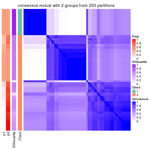
consensus_heatmap(res, k = 3)
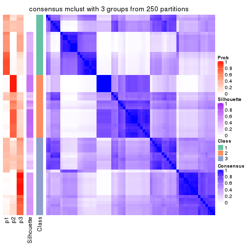
consensus_heatmap(res, k = 4)
consensus_heatmap(res, k = 5)
consensus_heatmap(res, k = 6)

Heatmaps for the membership of samples in all partitions to see how consistent they are:
membership_heatmap(res, k = 2)
membership_heatmap(res, k = 3)
membership_heatmap(res, k = 4)
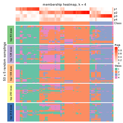
membership_heatmap(res, k = 5)
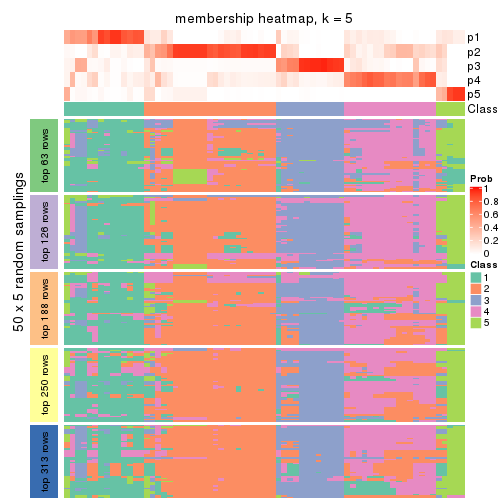
membership_heatmap(res, k = 6)
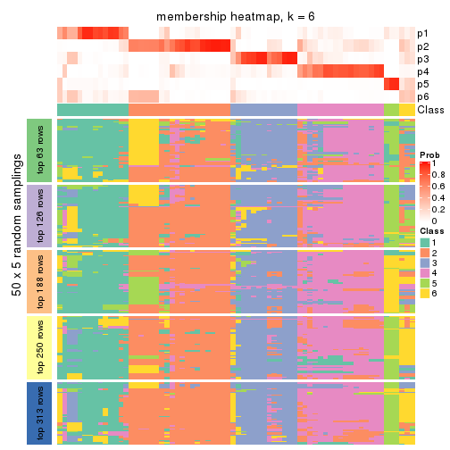
As soon as we have had the classes for columns, we can look for signatures which are significantly different between classes which can be candidate marks for certain classes. Following are the heatmaps for signatures.
Signature heatmaps where rows are scaled:
get_signatures(res, k = 2)
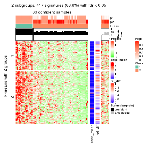
get_signatures(res, k = 3)
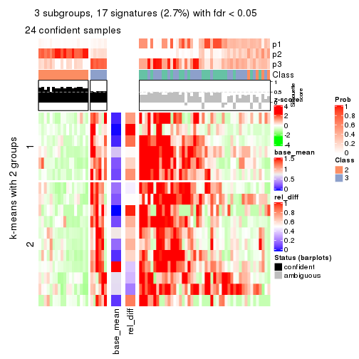
get_signatures(res, k = 4)
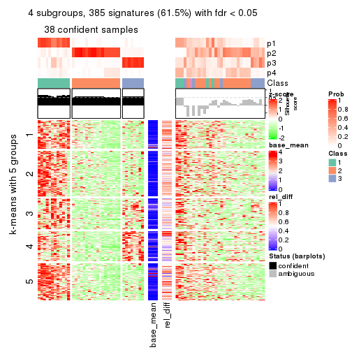
get_signatures(res, k = 5)
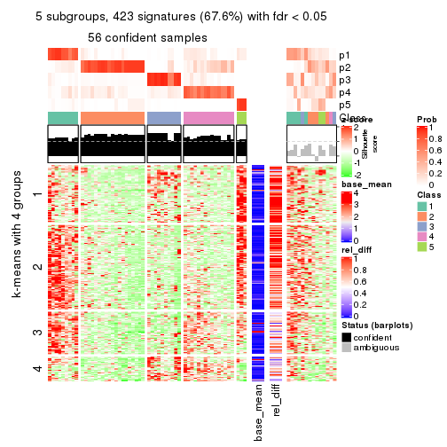
get_signatures(res, k = 6)
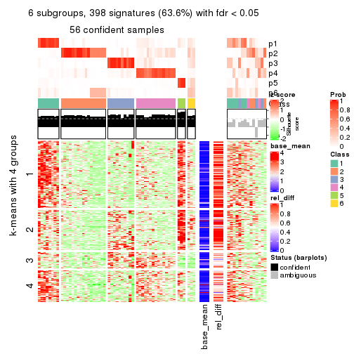
Signature heatmaps where rows are not scaled:
get_signatures(res, k = 2, scale_rows = FALSE)
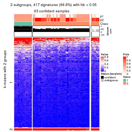
get_signatures(res, k = 3, scale_rows = FALSE)
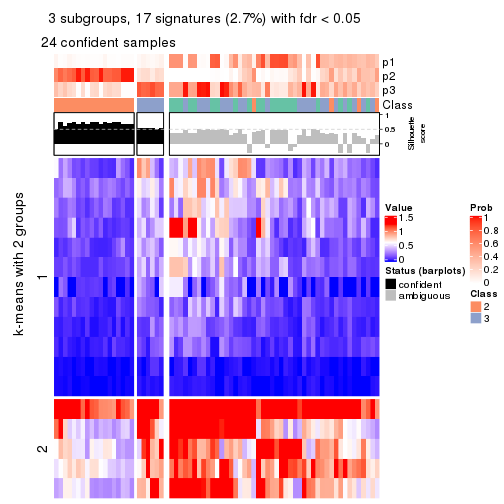
get_signatures(res, k = 4, scale_rows = FALSE)
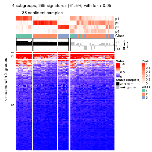
get_signatures(res, k = 5, scale_rows = FALSE)
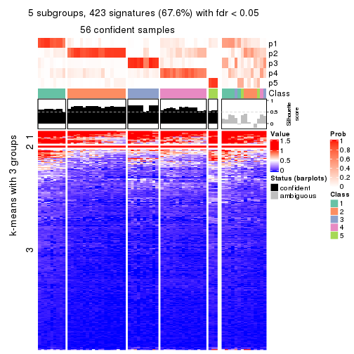
get_signatures(res, k = 6, scale_rows = FALSE)
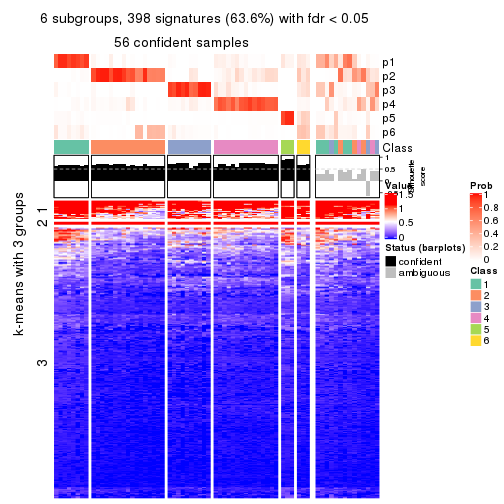
Compare the overlap of signatures from different k:
compare_signatures(res)
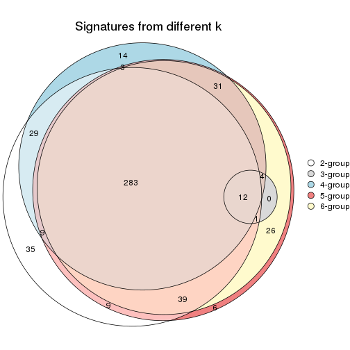
get_signature() returns a data frame invisibly. TO get the list of signatures, the function
call should be assigned to a variable explicitly. In following code, if plot argument is set
to FALSE, no heatmap is plotted while only the differential analysis is performed.
# code only for demonstration
tb = get_signature(res, k = ..., plot = FALSE)
An example of the output of tb is:
#>   which_row         fdr    mean_1    mean_2 scaled_mean_1 scaled_mean_2 km
#> 1        38 0.042760348  8.373488  9.131774    -0.5533452     0.5164555  1
#> 2        40 0.018707592  7.106213  8.469186    -0.6173731     0.5762149  1
#> 3        55 0.019134737 10.221463 11.207825    -0.6159697     0.5749050  1
#> 4        59 0.006059896  5.921854  7.869574    -0.6899429     0.6439467  1
#> 5        60 0.018055526  8.928898 10.211722    -0.6204761     0.5791110  1
#> 6        98 0.009384629 15.714769 14.887706     0.6635654    -0.6193277  2
...
The columns in tb are:
which_row: row indices corresponding to the input matrix.fdr: FDR for the differential test. mean_x: The mean value in group x.scaled_mean_x: The mean value in group x after rows are scaled.km: Row groups if k-means clustering is applied to rows.UMAP plot which shows how samples are separated.
dimension_reduction(res, k = 2, method = "UMAP")
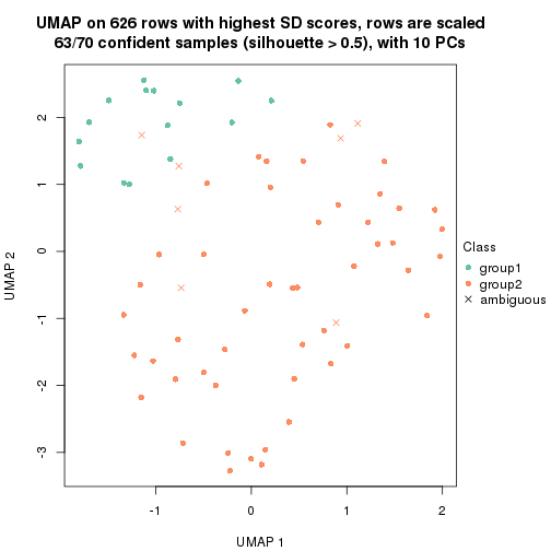
dimension_reduction(res, k = 3, method = "UMAP")
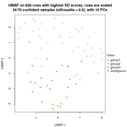
dimension_reduction(res, k = 4, method = "UMAP")
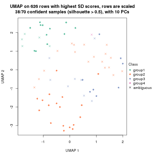
dimension_reduction(res, k = 5, method = "UMAP")
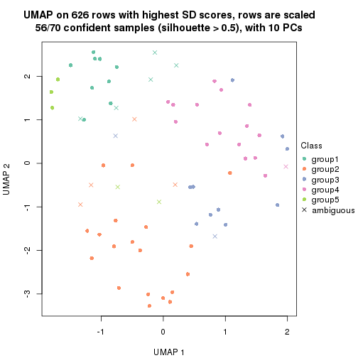
dimension_reduction(res, k = 6, method = "UMAP")
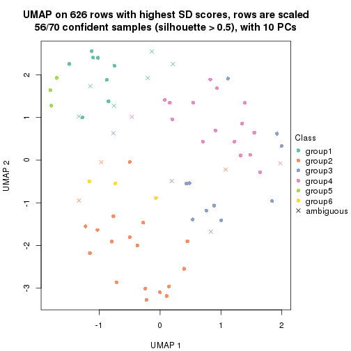
Following heatmap shows how subgroups are split when increasing k:
collect_classes(res)
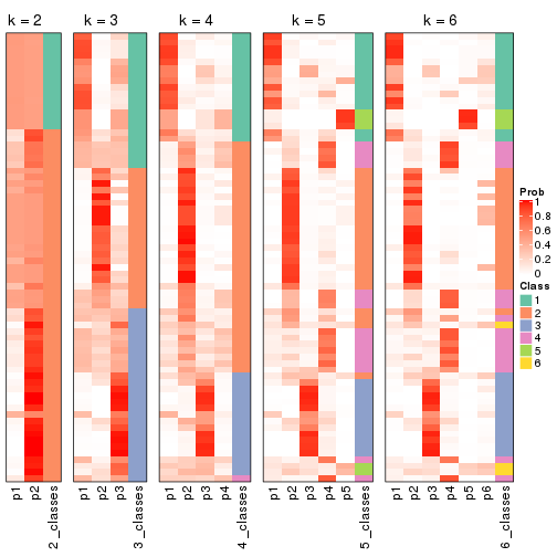
If matrix rows can be associated to genes, consider to use functional_enrichment(res,
...) to perform function enrichment for the signature genes. See this vignette for more detailed explanations.
The object with results only for a single top-value method and a single partition method can be extracted as:
res = res_list["SD", "NMF"]
# you can also extract it by
# res = res_list["SD:NMF"]
A summary of res and all the functions that can be applied to it:
res
#> A 'ConsensusPartition' object with k = 2, 3, 4, 5, 6.
#>   On a matrix with 626 rows and 70 columns.
#>   Top rows (63, 126, 188, 250, 313) are extracted by 'SD' method.
#>   Subgroups are detected by 'NMF' method.
#>   Performed in total 1250 partitions by row resampling.
#>   Best k for subgroups seems to be 2.
#>
#> Following methods can be applied to this 'ConsensusPartition' object:
#>  [1] "cola_report"             "collect_classes"         "collect_plots"
#>  [4] "collect_stats"           "colnames"                "compare_signatures"
#>  [7] "consensus_heatmap"       "dimension_reduction"     "functional_enrichment"
#> [10] "get_anno_col"            "get_anno"                "get_classes"
#> [13] "get_consensus"           "get_matrix"              "get_membership"
#> [16] "get_param"               "get_signatures"          "get_stats"
#> [19] "is_best_k"               "is_stable_k"             "membership_heatmap"
#> [22] "ncol"                    "nrow"                    "plot_ecdf"
#> [25] "rownames"                "select_partition_number" "show"
#> [28] "suggest_best_k"          "test_to_known_factors"
collect_plots() function collects all the plots made from res for all k (number of partitions)
into one single page to provide an easy and fast comparison between different k.
collect_plots(res)
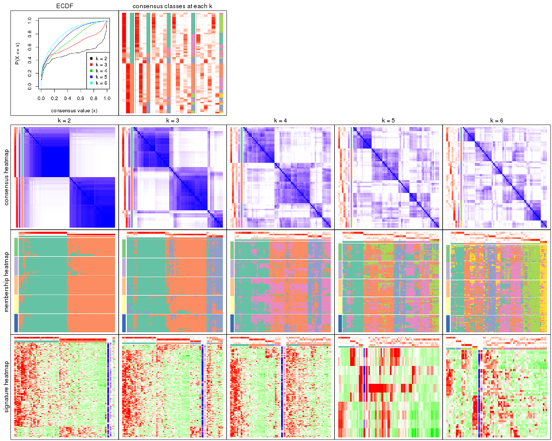
The plots are:
k and the heatmap of
predicted classes for each k.k.k.k.All the plots in panels can be made by individual functions and they are plotted later in this section.
select_partition_number() produces several plots showing different
statistics for choosing “optimized” k. There are following statistics:
k;k, the area increased is defined as \(A_k - A_{k-1}\).The detailed explanations of these statistics can be found in the cola vignette.
Generally speaking, lower PAC score, higher mean silhouette score or higher
concordance corresponds to better partition. Rand index and Jaccard index
measure how similar the current partition is compared to partition with k-1.
If they are too similar, we won't accept k is better than k-1.
select_partition_number(res)
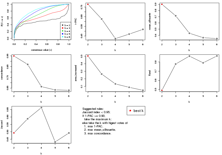
The numeric values for all these statistics can be obtained by get_stats().
get_stats(res)
#>   k 1-PAC mean_silhouette concordance area_increased  Rand Jaccard
#> 2 2 0.779           0.901       0.949         0.5032 0.493   0.493
#> 3 3 0.626           0.716       0.871         0.2631 0.778   0.588
#> 4 4 0.423           0.434       0.663         0.1320 0.864   0.663
#> 5 5 0.469           0.362       0.633         0.0870 0.791   0.432
#> 6 6 0.518           0.347       0.630         0.0478 0.865   0.492
suggest_best_k() suggests the best \(k\) based on these statistics. The rules are as follows:
suggest_best_k(res)
#> [1] 2
Following shows the table of the partitions (You need to click the show/hide
code output link to see it). The membership matrix (columns with name p*)
is inferred by
clue::cl_consensus()
function with the SE method. Basically the value in the membership matrix
represents the probability to belong to a certain group. The finall class
label for an item is determined with the group with highest probability it
belongs to.
In get_classes() function, the entropy is calculated from the membership
matrix and the silhouette score is calculated from the consensus matrix.
cbind(get_classes(res, k = 2), get_membership(res, k = 2))
#>           class entropy silhouette    p1    p2
#> SRR837437     2  0.2043      0.958 0.032 0.968
#> SRR837438     2  0.5842      0.869 0.140 0.860
#> SRR837439     2  0.4022      0.928 0.080 0.920
#> SRR837440     2  0.1414      0.962 0.020 0.980
#> SRR837441     2  0.3114      0.945 0.056 0.944
#> SRR837442     2  0.5178      0.895 0.116 0.884
#> SRR837443     2  0.0376      0.962 0.004 0.996
#> SRR837444     2  0.6343      0.828 0.160 0.840
#> SRR837445     1  0.0000      0.930 1.000 0.000
#> SRR837446     2  0.0000      0.961 0.000 1.000
#> SRR837447     1  0.0000      0.930 1.000 0.000
#> SRR837448     1  0.0938      0.925 0.988 0.012
#> SRR837449     1  0.0000      0.930 1.000 0.000
#> SRR837450     1  0.1633      0.919 0.976 0.024
#> SRR837451     2  0.1414      0.962 0.020 0.980
#> SRR837452     1  0.0000      0.930 1.000 0.000
#> SRR837453     2  0.5629      0.871 0.132 0.868
#> SRR837454     1  0.0000      0.930 1.000 0.000
#> SRR837455     1  0.0000      0.930 1.000 0.000
#> SRR837456     1  0.0000      0.930 1.000 0.000
#> SRR837457     2  0.0000      0.961 0.000 1.000
#> SRR837458     1  0.0000      0.930 1.000 0.000
#> SRR837459     2  0.0672      0.962 0.008 0.992
#> SRR837460     2  0.0376      0.962 0.004 0.996
#> SRR837461     2  0.1633      0.961 0.024 0.976
#> SRR837462     2  0.1414      0.962 0.020 0.980
#> SRR837463     2  0.2236      0.957 0.036 0.964
#> SRR837464     2  0.1633      0.961 0.024 0.976
#> SRR837465     1  0.3431      0.893 0.936 0.064
#> SRR837466     1  0.0000      0.930 1.000 0.000
#> SRR837467     2  0.2043      0.958 0.032 0.968
#> SRR837468     2  0.0000      0.961 0.000 1.000
#> SRR837469     2  0.6343      0.818 0.160 0.840
#> SRR837470     1  0.2236      0.915 0.964 0.036
#> SRR837471     1  0.0000      0.930 1.000 0.000
#> SRR837472     1  0.0000      0.930 1.000 0.000
#> SRR837473     1  0.0000      0.930 1.000 0.000
#> SRR837474     1  0.2043      0.914 0.968 0.032
#> SRR837475     1  0.0000      0.930 1.000 0.000
#> SRR837476     1  0.9661      0.380 0.608 0.392
#> SRR837477     1  0.2236      0.913 0.964 0.036
#> SRR837478     1  0.3879      0.889 0.924 0.076
#> SRR837479     2  0.0376      0.961 0.004 0.996
#> SRR837480     1  0.5946      0.834 0.856 0.144
#> SRR837481     2  0.0938      0.959 0.012 0.988
#> SRR837482     2  0.0376      0.961 0.004 0.996
#> SRR837483     1  0.7815      0.719 0.768 0.232
#> SRR837484     2  0.0000      0.961 0.000 1.000
#> SRR837485     2  0.0000      0.961 0.000 1.000
#> SRR837486     2  0.0000      0.961 0.000 1.000
#> SRR837487     2  0.3431      0.938 0.064 0.936
#> SRR837488     2  0.2043      0.959 0.032 0.968
#> SRR837489     1  0.9000      0.550 0.684 0.316
#> SRR837490     1  0.9710      0.343 0.600 0.400
#> SRR837491     1  0.9248      0.500 0.660 0.340
#> SRR837492     1  0.0000      0.930 1.000 0.000
#> SRR837493     2  0.4022      0.928 0.080 0.920
#> SRR837494     2  0.1633      0.961 0.024 0.976
#> SRR837495     1  0.0000      0.930 1.000 0.000
#> SRR837496     1  0.0000      0.930 1.000 0.000
#> SRR837497     1  0.0000      0.930 1.000 0.000
#> SRR837498     1  0.6148      0.809 0.848 0.152
#> SRR837499     1  0.0000      0.930 1.000 0.000
#> SRR837500     1  0.0000      0.930 1.000 0.000
#> SRR837501     2  0.0000      0.961 0.000 1.000
#> SRR837502     1  0.0000      0.930 1.000 0.000
#> SRR837503     1  0.0000      0.930 1.000 0.000
#> SRR837504     2  0.0000      0.961 0.000 1.000
#> SRR837505     2  0.0000      0.961 0.000 1.000
#> SRR837506     2  0.0000      0.961 0.000 1.000
cbind(get_classes(res, k = 3), get_membership(res, k = 3))
#>           class entropy silhouette    p1    p2    p3
#> SRR837437     2  0.0592     0.8400 0.012 0.988 0.000
#> SRR837438     2  0.2625     0.8084 0.084 0.916 0.000
#> SRR837439     2  0.1964     0.8261 0.056 0.944 0.000
#> SRR837440     2  0.1163     0.8360 0.000 0.972 0.028
#> SRR837441     2  0.1860     0.8276 0.052 0.948 0.000
#> SRR837442     2  0.2165     0.8243 0.064 0.936 0.000
#> SRR837443     2  0.0747     0.8397 0.000 0.984 0.016
#> SRR837444     2  0.3502     0.8057 0.084 0.896 0.020
#> SRR837445     1  0.2356     0.8497 0.928 0.072 0.000
#> SRR837446     3  0.5327     0.5815 0.000 0.272 0.728
#> SRR837447     1  0.0661     0.8694 0.988 0.004 0.008
#> SRR837448     1  0.5098     0.6383 0.752 0.000 0.248
#> SRR837449     1  0.1289     0.8711 0.968 0.032 0.000
#> SRR837450     1  0.6111     0.3441 0.604 0.000 0.396
#> SRR837451     2  0.0661     0.8408 0.008 0.988 0.004
#> SRR837452     1  0.0983     0.8719 0.980 0.016 0.004
#> SRR837453     2  0.4749     0.7720 0.076 0.852 0.072
#> SRR837454     1  0.1163     0.8718 0.972 0.028 0.000
#> SRR837455     1  0.1289     0.8708 0.968 0.032 0.000
#> SRR837456     1  0.1411     0.8697 0.964 0.036 0.000
#> SRR837457     2  0.1529     0.8317 0.000 0.960 0.040
#> SRR837458     1  0.0983     0.8670 0.980 0.004 0.016
#> SRR837459     2  0.1163     0.8377 0.000 0.972 0.028
#> SRR837460     2  0.1643     0.8285 0.000 0.956 0.044
#> SRR837461     2  0.0892     0.8381 0.000 0.980 0.020
#> SRR837462     2  0.1182     0.8417 0.012 0.976 0.012
#> SRR837463     2  0.1163     0.8364 0.028 0.972 0.000
#> SRR837464     2  0.1289     0.8342 0.000 0.968 0.032
#> SRR837465     1  0.5621     0.5484 0.692 0.308 0.000
#> SRR837466     1  0.3116     0.8091 0.892 0.000 0.108
#> SRR837467     2  0.1031     0.8376 0.024 0.976 0.000
#> SRR837468     2  0.5948     0.3695 0.000 0.640 0.360
#> SRR837469     2  0.7213     0.5135 0.060 0.668 0.272
#> SRR837470     1  0.5072     0.7135 0.792 0.012 0.196
#> SRR837471     1  0.1289     0.8711 0.968 0.032 0.000
#> SRR837472     1  0.1163     0.8714 0.972 0.028 0.000
#> SRR837473     1  0.1289     0.8592 0.968 0.000 0.032
#> SRR837474     1  0.3267     0.8095 0.884 0.116 0.000
#> SRR837475     1  0.1289     0.8592 0.968 0.000 0.032
#> SRR837476     2  0.6204     0.2554 0.424 0.576 0.000
#> SRR837477     3  0.6309    -0.1020 0.496 0.000 0.504
#> SRR837478     3  0.2261     0.7357 0.068 0.000 0.932
#> SRR837479     3  0.1529     0.7714 0.000 0.040 0.960
#> SRR837480     3  0.1529     0.7517 0.040 0.000 0.960
#> SRR837481     3  0.1289     0.7708 0.000 0.032 0.968
#> SRR837482     2  0.6204     0.2156 0.000 0.576 0.424
#> SRR837483     3  0.8065     0.4066 0.304 0.092 0.604
#> SRR837484     3  0.6291     0.1364 0.000 0.468 0.532
#> SRR837485     3  0.2448     0.7673 0.000 0.076 0.924
#> SRR837486     3  0.2625     0.7653 0.000 0.084 0.916
#> SRR837487     2  0.4558     0.7763 0.044 0.856 0.100
#> SRR837488     2  0.1964     0.8213 0.000 0.944 0.056
#> SRR837489     1  0.6286     0.0967 0.536 0.464 0.000
#> SRR837490     2  0.6062     0.3791 0.384 0.616 0.000
#> SRR837491     2  0.6280     0.1444 0.460 0.540 0.000
#> SRR837492     1  0.3340     0.7981 0.880 0.000 0.120
#> SRR837493     2  0.2537     0.8111 0.080 0.920 0.000
#> SRR837494     2  0.0424     0.8401 0.000 0.992 0.008
#> SRR837495     1  0.0475     0.8694 0.992 0.004 0.004
#> SRR837496     1  0.1964     0.8454 0.944 0.000 0.056
#> SRR837497     1  0.1289     0.8596 0.968 0.000 0.032
#> SRR837498     1  0.5859     0.4745 0.656 0.344 0.000
#> SRR837499     1  0.1753     0.8645 0.952 0.048 0.000
#> SRR837500     1  0.1529     0.8680 0.960 0.040 0.000
#> SRR837501     2  0.3686     0.7501 0.000 0.860 0.140
#> SRR837502     1  0.1860     0.8623 0.948 0.052 0.000
#> SRR837503     1  0.1163     0.8611 0.972 0.000 0.028
#> SRR837504     2  0.2066     0.8199 0.000 0.940 0.060
#> SRR837505     3  0.5859     0.4720 0.000 0.344 0.656
#> SRR837506     3  0.2448     0.7664 0.000 0.076 0.924
cbind(get_classes(res, k = 4), get_membership(res, k = 4))
#>           class entropy silhouette    p1    p2    p3    p4
#> SRR837437     2  0.4248     0.4835 0.012 0.768 0.000 0.220
#> SRR837438     2  0.5769     0.1033 0.036 0.588 0.000 0.376
#> SRR837439     2  0.5174     0.1675 0.012 0.620 0.000 0.368
#> SRR837440     2  0.3266     0.5415 0.000 0.832 0.000 0.168
#> SRR837441     2  0.5149     0.2835 0.016 0.648 0.000 0.336
#> SRR837442     2  0.5288     0.4569 0.056 0.720 0.000 0.224
#> SRR837443     2  0.4522     0.3739 0.000 0.680 0.000 0.320
#> SRR837444     4  0.7773     0.5362 0.068 0.320 0.076 0.536
#> SRR837445     4  0.8174     0.6208 0.208 0.208 0.048 0.536
#> SRR837446     3  0.5756     0.5183 0.000 0.084 0.692 0.224
#> SRR837447     1  0.5721     0.4810 0.584 0.024 0.004 0.388
#> SRR837448     1  0.4635     0.5132 0.756 0.000 0.216 0.028
#> SRR837449     1  0.4936     0.5810 0.672 0.012 0.000 0.316
#> SRR837450     1  0.5682     0.2693 0.612 0.000 0.352 0.036
#> SRR837451     2  0.3356     0.5194 0.000 0.824 0.000 0.176
#> SRR837452     1  0.6686     0.4358 0.560 0.076 0.008 0.356
#> SRR837453     2  0.7062     0.1430 0.028 0.584 0.080 0.308
#> SRR837454     1  0.7085     0.1852 0.468 0.096 0.008 0.428
#> SRR837455     1  0.4008     0.6304 0.756 0.000 0.000 0.244
#> SRR837456     1  0.3907     0.6353 0.768 0.000 0.000 0.232
#> SRR837457     2  0.3032     0.5700 0.000 0.868 0.008 0.124
#> SRR837458     1  0.2125     0.6563 0.932 0.012 0.004 0.052
#> SRR837459     2  0.3808     0.5453 0.004 0.824 0.012 0.160
#> SRR837460     2  0.2401     0.5843 0.000 0.904 0.004 0.092
#> SRR837461     2  0.1302     0.5800 0.000 0.956 0.000 0.044
#> SRR837462     2  0.4454     0.3269 0.000 0.692 0.000 0.308
#> SRR837463     2  0.1389     0.5767 0.000 0.952 0.000 0.048
#> SRR837464     2  0.1716     0.5785 0.000 0.936 0.000 0.064
#> SRR837465     4  0.7902     0.4345 0.300 0.260 0.004 0.436
#> SRR837466     1  0.2385     0.6465 0.920 0.000 0.052 0.028
#> SRR837467     2  0.2149     0.5637 0.000 0.912 0.000 0.088
#> SRR837468     2  0.7427     0.0693 0.000 0.500 0.200 0.300
#> SRR837469     4  0.8498     0.3598 0.060 0.316 0.156 0.468
#> SRR837470     1  0.8797     0.2638 0.392 0.064 0.180 0.364
#> SRR837471     1  0.1389     0.6622 0.952 0.000 0.000 0.048
#> SRR837472     1  0.1042     0.6567 0.972 0.008 0.000 0.020
#> SRR837473     1  0.0376     0.6588 0.992 0.000 0.004 0.004
#> SRR837474     1  0.5113     0.5795 0.760 0.088 0.000 0.152
#> SRR837475     1  0.1042     0.6640 0.972 0.000 0.008 0.020
#> SRR837476     2  0.7253    -0.4079 0.152 0.484 0.000 0.364
#> SRR837477     3  0.5453     0.3971 0.320 0.000 0.648 0.032
#> SRR837478     3  0.3958     0.6526 0.144 0.000 0.824 0.032
#> SRR837479     3  0.1543     0.6986 0.004 0.008 0.956 0.032
#> SRR837480     3  0.3278     0.6716 0.116 0.000 0.864 0.020
#> SRR837481     3  0.1174     0.6968 0.000 0.012 0.968 0.020
#> SRR837482     3  0.7024     0.2275 0.000 0.360 0.512 0.128
#> SRR837483     1  0.8696    -0.0885 0.476 0.072 0.180 0.272
#> SRR837484     2  0.7630     0.0948 0.000 0.460 0.228 0.312
#> SRR837485     3  0.5976     0.6471 0.004 0.096 0.692 0.208
#> SRR837486     3  0.8529     0.4601 0.044 0.228 0.464 0.264
#> SRR837487     2  0.7012     0.4130 0.036 0.604 0.072 0.288
#> SRR837488     2  0.4778     0.5111 0.004 0.732 0.016 0.248
#> SRR837489     4  0.7387     0.4886 0.144 0.384 0.004 0.468
#> SRR837490     4  0.7250     0.5962 0.160 0.336 0.000 0.504
#> SRR837491     2  0.7502    -0.3825 0.188 0.456 0.000 0.356
#> SRR837492     1  0.2773     0.6319 0.900 0.000 0.072 0.028
#> SRR837493     2  0.5536    -0.0465 0.024 0.592 0.000 0.384
#> SRR837494     2  0.2081     0.5782 0.000 0.916 0.000 0.084
#> SRR837495     1  0.7335     0.2642 0.496 0.028 0.080 0.396
#> SRR837496     1  0.7337     0.4446 0.524 0.000 0.204 0.272
#> SRR837497     1  0.5802     0.4195 0.568 0.020 0.008 0.404
#> SRR837498     4  0.7369     0.6210 0.196 0.292 0.000 0.512
#> SRR837499     1  0.5856     0.3035 0.556 0.036 0.000 0.408
#> SRR837500     1  0.4008     0.6165 0.756 0.000 0.000 0.244
#> SRR837501     2  0.5578     0.3988 0.000 0.648 0.040 0.312
#> SRR837502     1  0.4917     0.4995 0.656 0.008 0.000 0.336
#> SRR837503     1  0.2831     0.6529 0.876 0.000 0.004 0.120
#> SRR837504     2  0.3895     0.5429 0.000 0.804 0.012 0.184
#> SRR837505     2  0.7869    -0.2042 0.000 0.392 0.296 0.312
#> SRR837506     3  0.7118     0.5168 0.000 0.156 0.536 0.308
cbind(get_classes(res, k = 5), get_membership(res, k = 5))
#>           class entropy silhouette    p1    p2    p3    p4    p5
#> SRR837437     2  0.3297    0.48626 0.000 0.860 0.012 0.048 0.080
#> SRR837438     2  0.5426    0.36737 0.012 0.688 0.048 0.232 0.020
#> SRR837439     2  0.4556    0.35558 0.000 0.680 0.024 0.292 0.004
#> SRR837440     2  0.4141    0.51220 0.000 0.788 0.008 0.152 0.052
#> SRR837441     2  0.3815    0.48870 0.000 0.764 0.012 0.220 0.004
#> SRR837442     2  0.5108    0.41458 0.096 0.760 0.012 0.028 0.104
#> SRR837443     2  0.4636    0.49341 0.000 0.756 0.060 0.168 0.016
#> SRR837444     4  0.7644    0.11341 0.020 0.336 0.264 0.364 0.016
#> SRR837445     4  0.8662    0.14817 0.124 0.296 0.244 0.320 0.016
#> SRR837446     3  0.6300    0.40149 0.000 0.148 0.644 0.152 0.056
#> SRR837447     4  0.3430    0.46431 0.220 0.000 0.004 0.776 0.000
#> SRR837448     1  0.4809    0.48185 0.704 0.000 0.240 0.048 0.008
#> SRR837449     4  0.4181    0.36600 0.316 0.004 0.000 0.676 0.004
#> SRR837450     1  0.5894    0.25489 0.584 0.000 0.328 0.028 0.060
#> SRR837451     2  0.6514    0.29377 0.000 0.480 0.008 0.356 0.156
#> SRR837452     4  0.4871    0.43125 0.256 0.016 0.012 0.700 0.016
#> SRR837453     4  0.7553   -0.08697 0.012 0.308 0.092 0.488 0.100
#> SRR837454     4  0.3381    0.50314 0.160 0.000 0.004 0.820 0.016
#> SRR837455     4  0.4554    0.32292 0.340 0.004 0.004 0.644 0.008
#> SRR837456     4  0.4480    0.22756 0.400 0.004 0.000 0.592 0.004
#> SRR837457     2  0.6434    0.16575 0.000 0.444 0.004 0.152 0.400
#> SRR837458     1  0.1282    0.68635 0.952 0.000 0.000 0.044 0.004
#> SRR837459     2  0.6787    0.23589 0.000 0.380 0.000 0.332 0.288
#> SRR837460     2  0.6516    0.22771 0.000 0.492 0.012 0.144 0.352
#> SRR837461     2  0.5345    0.37670 0.000 0.632 0.000 0.088 0.280
#> SRR837462     4  0.6640   -0.13207 0.000 0.312 0.004 0.472 0.212
#> SRR837463     2  0.5180    0.44005 0.004 0.696 0.000 0.112 0.188
#> SRR837464     2  0.5523    0.32966 0.000 0.592 0.000 0.088 0.320
#> SRR837465     4  0.5486    0.52667 0.132 0.092 0.020 0.732 0.024
#> SRR837466     1  0.1310    0.69005 0.956 0.000 0.020 0.024 0.000
#> SRR837467     2  0.4971    0.45473 0.000 0.708 0.000 0.116 0.176
#> SRR837468     5  0.5126    0.55743 0.000 0.128 0.064 0.060 0.748
#> SRR837469     4  0.6431    0.43495 0.020 0.072 0.140 0.672 0.096
#> SRR837470     4  0.7069    0.43921 0.156 0.008 0.104 0.600 0.132
#> SRR837471     1  0.1197    0.69109 0.952 0.000 0.000 0.048 0.000
#> SRR837472     1  0.0324    0.69417 0.992 0.004 0.000 0.004 0.000
#> SRR837473     1  0.0566    0.69445 0.984 0.000 0.004 0.012 0.000
#> SRR837474     1  0.4981    0.50284 0.740 0.156 0.012 0.088 0.004
#> SRR837475     1  0.1341    0.68561 0.944 0.000 0.000 0.056 0.000
#> SRR837476     4  0.7209    0.18716 0.060 0.308 0.024 0.528 0.080
#> SRR837477     3  0.4135    0.41471 0.340 0.000 0.656 0.004 0.000
#> SRR837478     3  0.2921    0.59836 0.124 0.000 0.856 0.000 0.020
#> SRR837479     3  0.2890    0.53539 0.000 0.000 0.836 0.004 0.160
#> SRR837480     3  0.3340    0.60119 0.124 0.004 0.840 0.000 0.032
#> SRR837481     3  0.2037    0.57326 0.000 0.004 0.920 0.012 0.064
#> SRR837482     3  0.6105    0.29766 0.000 0.248 0.620 0.032 0.100
#> SRR837483     1  0.6979    0.32757 0.636 0.096 0.096 0.032 0.140
#> SRR837484     5  0.7377    0.30670 0.000 0.356 0.204 0.040 0.400
#> SRR837485     3  0.5720    0.03184 0.000 0.036 0.536 0.028 0.400
#> SRR837486     5  0.7955    0.25559 0.040 0.180 0.304 0.036 0.440
#> SRR837487     2  0.7339    0.07097 0.072 0.560 0.072 0.040 0.256
#> SRR837488     2  0.5553    0.30421 0.016 0.684 0.028 0.040 0.232
#> SRR837489     2  0.6709    0.33385 0.056 0.592 0.052 0.272 0.028
#> SRR837490     2  0.6558    0.02405 0.052 0.488 0.036 0.408 0.016
#> SRR837491     2  0.6600    0.37137 0.136 0.636 0.028 0.172 0.028
#> SRR837492     1  0.1455    0.68686 0.952 0.000 0.032 0.008 0.008
#> SRR837493     2  0.5565    0.20746 0.000 0.544 0.020 0.400 0.036
#> SRR837494     2  0.4042    0.43687 0.000 0.756 0.000 0.032 0.212
#> SRR837495     4  0.8775    0.19336 0.236 0.172 0.224 0.352 0.016
#> SRR837496     3  0.8459   -0.00452 0.308 0.108 0.364 0.204 0.016
#> SRR837497     4  0.7214    0.31132 0.240 0.128 0.064 0.556 0.012
#> SRR837498     4  0.4945    0.44824 0.032 0.188 0.032 0.740 0.008
#> SRR837499     1  0.7786   -0.11504 0.408 0.168 0.052 0.356 0.016
#> SRR837500     1  0.5961    0.15291 0.548 0.076 0.016 0.360 0.000
#> SRR837501     5  0.4353    0.51467 0.000 0.224 0.024 0.012 0.740
#> SRR837502     1  0.7552   -0.01850 0.444 0.160 0.040 0.340 0.016
#> SRR837503     1  0.4826    0.57274 0.784 0.048 0.040 0.112 0.016
#> SRR837504     5  0.5811    0.08839 0.000 0.348 0.004 0.092 0.556
#> SRR837505     5  0.3216    0.58707 0.000 0.068 0.048 0.016 0.868
#> SRR837506     5  0.3550    0.32280 0.000 0.000 0.236 0.004 0.760
cbind(get_classes(res, k = 6), get_membership(res, k = 6))
#>           class entropy silhouette    p1    p2    p3    p4    p5    p6
#> SRR837437     4  0.4406   -0.18223 0.000 0.476 0.000 0.500 0.000 0.024
#> SRR837438     4  0.3470    0.34384 0.020 0.148 0.000 0.812 0.012 0.008
#> SRR837439     4  0.3078    0.34775 0.032 0.104 0.000 0.848 0.000 0.016
#> SRR837440     4  0.4122    0.18468 0.008 0.172 0.000 0.752 0.000 0.068
#> SRR837441     4  0.3141    0.30682 0.012 0.140 0.000 0.828 0.000 0.020
#> SRR837442     2  0.5443    0.26119 0.000 0.556 0.000 0.324 0.112 0.008
#> SRR837443     4  0.3859    0.21080 0.000 0.204 0.024 0.756 0.000 0.016
#> SRR837444     4  0.4122    0.36206 0.068 0.000 0.172 0.752 0.008 0.000
#> SRR837445     4  0.6498    0.24339 0.060 0.020 0.156 0.580 0.184 0.000
#> SRR837446     3  0.4104    0.42894 0.000 0.008 0.664 0.316 0.004 0.008
#> SRR837447     1  0.2448    0.70001 0.884 0.000 0.000 0.052 0.064 0.000
#> SRR837448     5  0.6166    0.35624 0.080 0.064 0.272 0.000 0.572 0.012
#> SRR837449     1  0.2670    0.70238 0.872 0.004 0.000 0.040 0.084 0.000
#> SRR837450     5  0.7014    0.23237 0.064 0.076 0.300 0.000 0.496 0.064
#> SRR837451     2  0.7152    0.27175 0.308 0.408 0.000 0.156 0.000 0.128
#> SRR837452     1  0.2800    0.68629 0.880 0.060 0.012 0.008 0.040 0.000
#> SRR837453     1  0.7155   -0.01946 0.452 0.320 0.072 0.124 0.000 0.032
#> SRR837454     1  0.2577    0.69996 0.888 0.016 0.000 0.056 0.040 0.000
#> SRR837455     1  0.2588    0.70030 0.860 0.004 0.000 0.012 0.124 0.000
#> SRR837456     1  0.3320    0.60431 0.772 0.000 0.000 0.016 0.212 0.000
#> SRR837457     2  0.7573    0.15297 0.124 0.308 0.004 0.268 0.000 0.296
#> SRR837458     5  0.2249    0.67665 0.064 0.032 0.000 0.000 0.900 0.004
#> SRR837459     4  0.7670   -0.26852 0.204 0.176 0.004 0.340 0.000 0.276
#> SRR837460     2  0.7536    0.24394 0.148 0.404 0.008 0.192 0.000 0.248
#> SRR837461     4  0.6827   -0.33275 0.052 0.340 0.000 0.384 0.000 0.224
#> SRR837462     4  0.7532   -0.11676 0.296 0.164 0.004 0.364 0.000 0.172
#> SRR837463     2  0.7172    0.34034 0.160 0.388 0.000 0.328 0.000 0.124
#> SRR837464     2  0.7338    0.24530 0.112 0.364 0.000 0.268 0.000 0.256
#> SRR837465     1  0.5910    0.56346 0.680 0.068 0.012 0.152 0.048 0.040
#> SRR837466     5  0.2659    0.66525 0.020 0.032 0.028 0.000 0.896 0.024
#> SRR837467     2  0.7188    0.33792 0.124 0.404 0.000 0.328 0.004 0.140
#> SRR837468     6  0.5033    0.62905 0.040 0.116 0.024 0.084 0.000 0.736
#> SRR837469     1  0.7485    0.42781 0.532 0.052 0.120 0.180 0.012 0.104
#> SRR837470     1  0.8592    0.33110 0.444 0.064 0.112 0.112 0.076 0.192
#> SRR837471     5  0.1577    0.68955 0.036 0.008 0.000 0.016 0.940 0.000
#> SRR837472     5  0.1269    0.68638 0.012 0.020 0.000 0.012 0.956 0.000
#> SRR837473     5  0.0717    0.68808 0.016 0.008 0.000 0.000 0.976 0.000
#> SRR837474     5  0.5561    0.48585 0.060 0.064 0.000 0.204 0.660 0.012
#> SRR837475     5  0.1707    0.68914 0.056 0.004 0.000 0.012 0.928 0.000
#> SRR837476     4  0.6746    0.16070 0.312 0.228 0.000 0.424 0.020 0.016
#> SRR837477     3  0.4040    0.40874 0.004 0.000 0.676 0.012 0.304 0.004
#> SRR837478     3  0.1734    0.61492 0.004 0.008 0.932 0.008 0.048 0.000
#> SRR837479     3  0.1787    0.58052 0.004 0.000 0.920 0.008 0.000 0.068
#> SRR837480     3  0.2723    0.61316 0.008 0.000 0.872 0.016 0.096 0.008
#> SRR837481     3  0.2773    0.58258 0.004 0.128 0.852 0.000 0.004 0.012
#> SRR837482     3  0.5063    0.19556 0.004 0.456 0.484 0.052 0.000 0.004
#> SRR837483     5  0.4633    0.39982 0.000 0.320 0.016 0.004 0.636 0.024
#> SRR837484     2  0.4767    0.28969 0.012 0.752 0.104 0.044 0.000 0.088
#> SRR837485     3  0.6499    0.18905 0.016 0.384 0.404 0.012 0.000 0.184
#> SRR837486     2  0.5568    0.07172 0.000 0.660 0.156 0.008 0.036 0.140
#> SRR837487     2  0.4337    0.36311 0.000 0.796 0.028 0.076 0.052 0.048
#> SRR837488     2  0.3058    0.41123 0.000 0.836 0.004 0.136 0.008 0.016
#> SRR837489     2  0.6746    0.11567 0.164 0.396 0.020 0.392 0.028 0.000
#> SRR837490     4  0.6922    0.12315 0.224 0.240 0.024 0.476 0.036 0.000
#> SRR837491     2  0.6676    0.11652 0.100 0.412 0.008 0.404 0.076 0.000
#> SRR837492     5  0.1427    0.67567 0.004 0.024 0.012 0.004 0.952 0.004
#> SRR837493     4  0.4654    0.35370 0.152 0.104 0.000 0.724 0.000 0.020
#> SRR837494     2  0.5682    0.26617 0.016 0.448 0.000 0.436 0.000 0.100
#> SRR837495     4  0.7106    0.04462 0.100 0.000 0.216 0.428 0.256 0.000
#> SRR837496     3  0.6792    0.08470 0.044 0.000 0.360 0.352 0.244 0.000
#> SRR837497     4  0.6418   -0.01625 0.376 0.008 0.020 0.444 0.148 0.004
#> SRR837498     4  0.4891    0.04587 0.420 0.016 0.004 0.536 0.024 0.000
#> SRR837499     4  0.6271    0.02871 0.232 0.004 0.008 0.444 0.312 0.000
#> SRR837500     5  0.5903   -0.03329 0.396 0.000 0.000 0.204 0.400 0.000
#> SRR837501     6  0.4140    0.69618 0.024 0.072 0.004 0.116 0.000 0.784
#> SRR837502     5  0.7087    0.00731 0.296 0.024 0.016 0.328 0.332 0.004
#> SRR837503     5  0.4473    0.53651 0.072 0.000 0.008 0.212 0.708 0.000
#> SRR837504     6  0.5127    0.46229 0.004 0.096 0.008 0.252 0.000 0.640
#> SRR837505     6  0.1370    0.72178 0.004 0.036 0.000 0.012 0.000 0.948
#> SRR837506     6  0.2463    0.63280 0.004 0.024 0.080 0.000 0.004 0.888
Heatmaps for the consensus matrix. It visualizes the probability of two samples to be in a same group.
consensus_heatmap(res, k = 2)
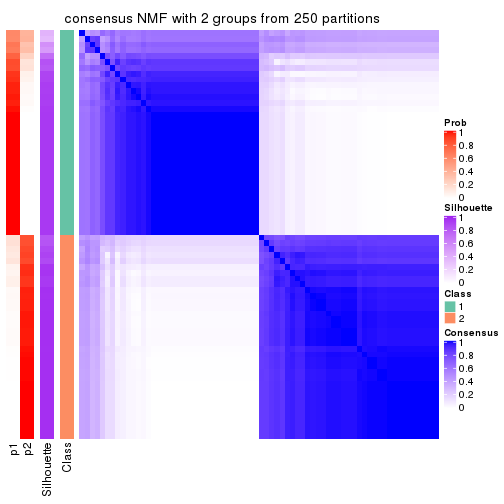
consensus_heatmap(res, k = 3)
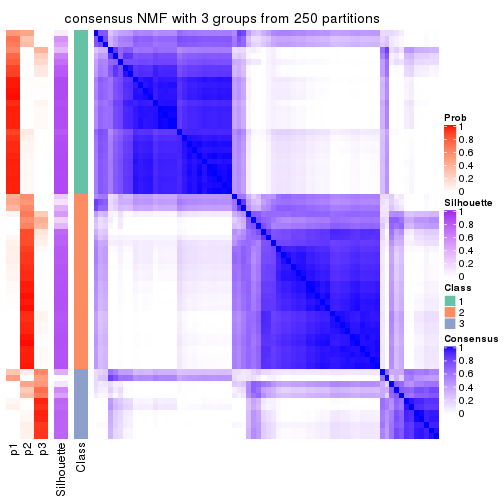
consensus_heatmap(res, k = 4)
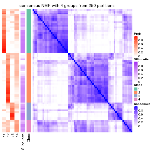
consensus_heatmap(res, k = 5)
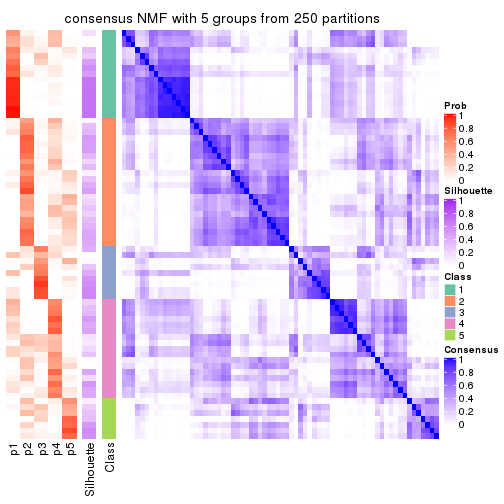
consensus_heatmap(res, k = 6)
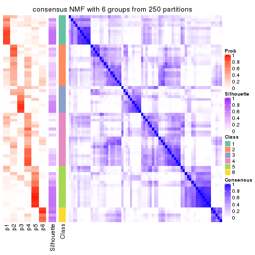
Heatmaps for the membership of samples in all partitions to see how consistent they are:
membership_heatmap(res, k = 2)

membership_heatmap(res, k = 3)
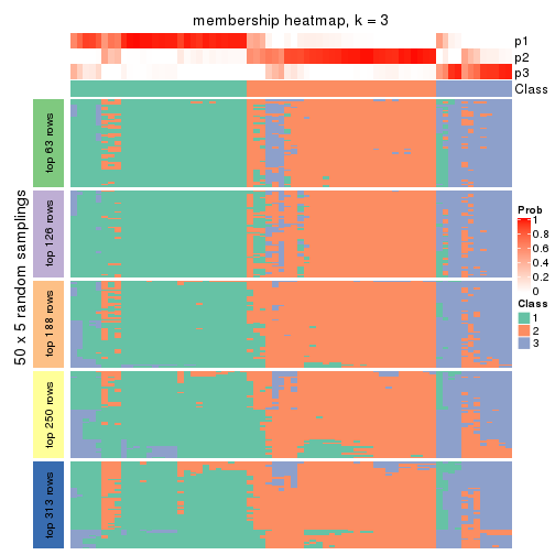
membership_heatmap(res, k = 4)
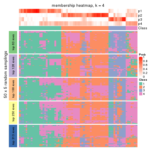
membership_heatmap(res, k = 5)
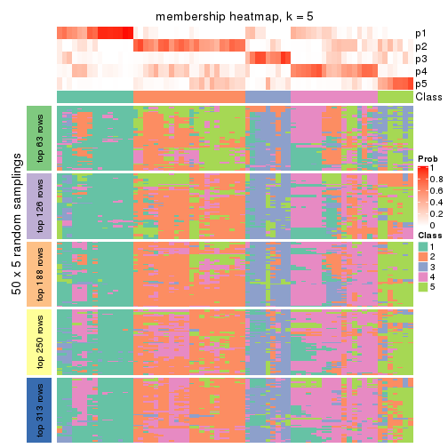
membership_heatmap(res, k = 6)
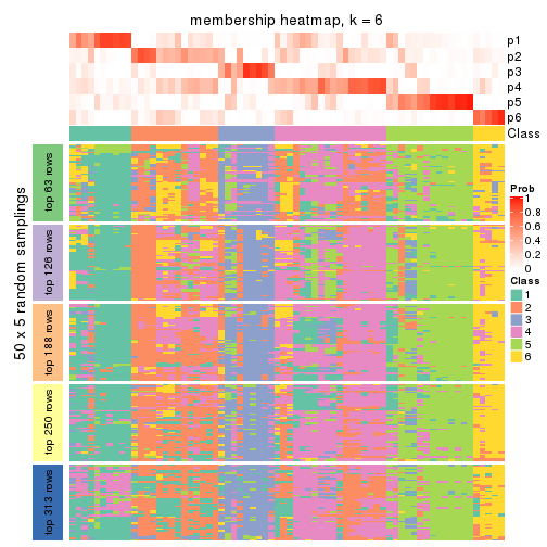
As soon as we have had the classes for columns, we can look for signatures which are significantly different between classes which can be candidate marks for certain classes. Following are the heatmaps for signatures.
Signature heatmaps where rows are scaled:
get_signatures(res, k = 2)
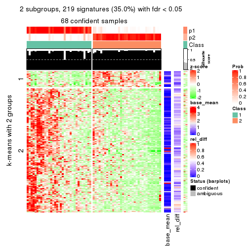
get_signatures(res, k = 3)
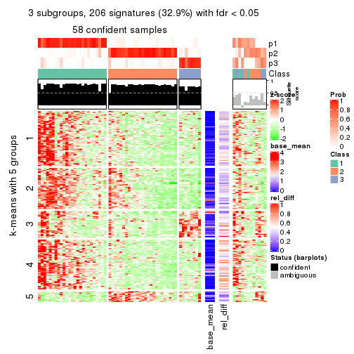
get_signatures(res, k = 4)
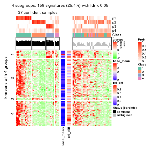
get_signatures(res, k = 5)
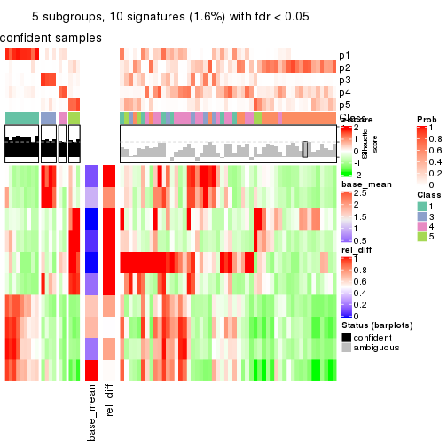
get_signatures(res, k = 6)
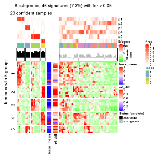
Signature heatmaps where rows are not scaled:
get_signatures(res, k = 2, scale_rows = FALSE)
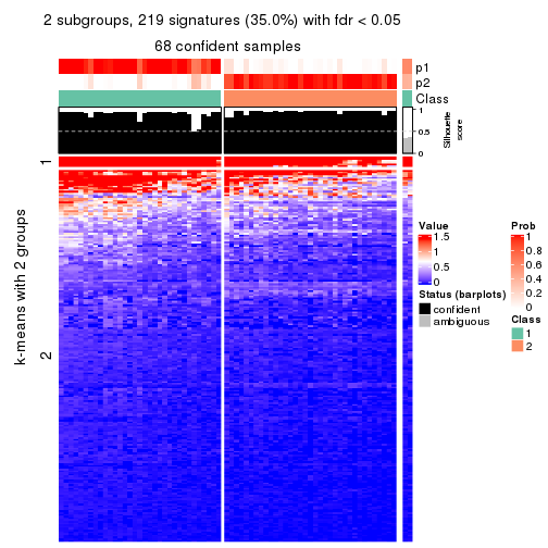
get_signatures(res, k = 3, scale_rows = FALSE)
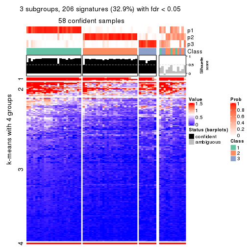
get_signatures(res, k = 4, scale_rows = FALSE)
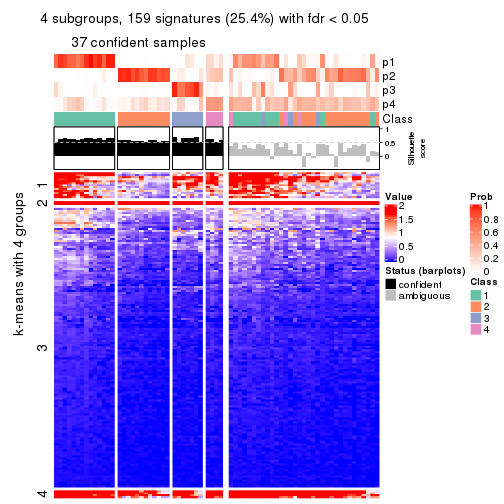
get_signatures(res, k = 5, scale_rows = FALSE)
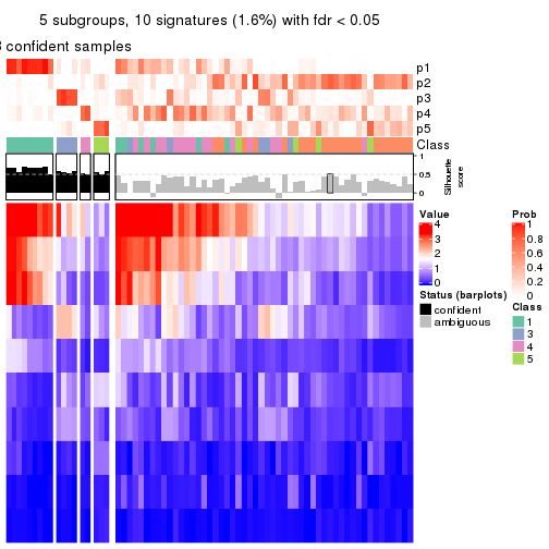
get_signatures(res, k = 6, scale_rows = FALSE)
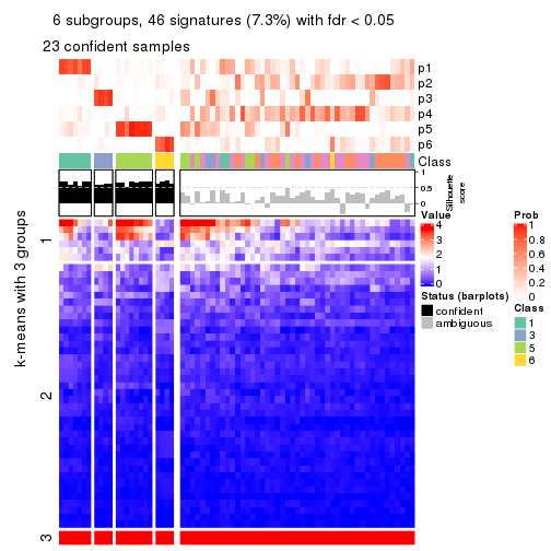
Compare the overlap of signatures from different k:
compare_signatures(res)
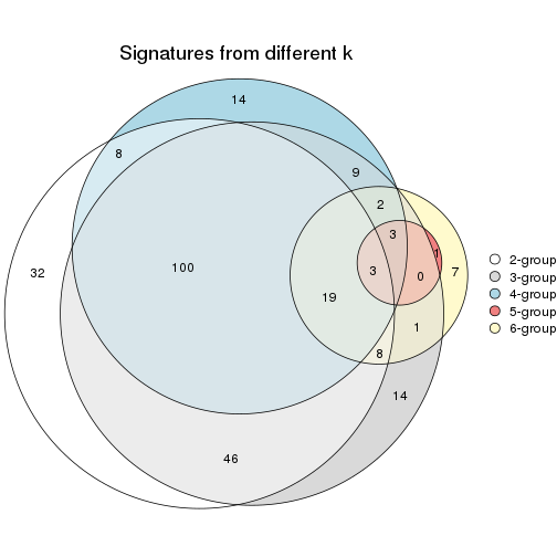
get_signature() returns a data frame invisibly. TO get the list of signatures, the function
call should be assigned to a variable explicitly. In following code, if plot argument is set
to FALSE, no heatmap is plotted while only the differential analysis is performed.
# code only for demonstration
tb = get_signature(res, k = ..., plot = FALSE)
An example of the output of tb is:
#>   which_row         fdr    mean_1    mean_2 scaled_mean_1 scaled_mean_2 km
#> 1        38 0.042760348  8.373488  9.131774    -0.5533452     0.5164555  1
#> 2        40 0.018707592  7.106213  8.469186    -0.6173731     0.5762149  1
#> 3        55 0.019134737 10.221463 11.207825    -0.6159697     0.5749050  1
#> 4        59 0.006059896  5.921854  7.869574    -0.6899429     0.6439467  1
#> 5        60 0.018055526  8.928898 10.211722    -0.6204761     0.5791110  1
#> 6        98 0.009384629 15.714769 14.887706     0.6635654    -0.6193277  2
...
The columns in tb are:
which_row: row indices corresponding to the input matrix.fdr: FDR for the differential test. mean_x: The mean value in group x.scaled_mean_x: The mean value in group x after rows are scaled.km: Row groups if k-means clustering is applied to rows.UMAP plot which shows how samples are separated.
dimension_reduction(res, k = 2, method = "UMAP")
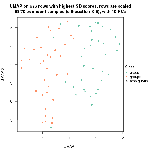
dimension_reduction(res, k = 3, method = "UMAP")
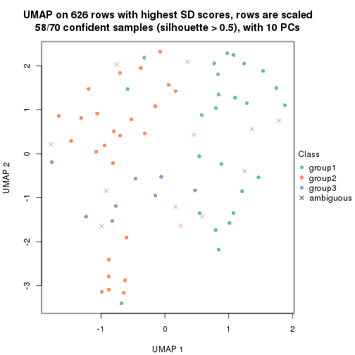
dimension_reduction(res, k = 4, method = "UMAP")
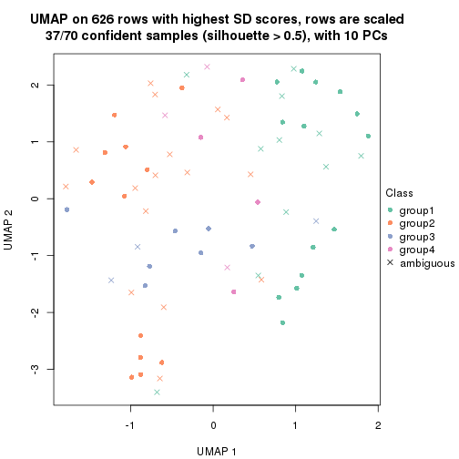
dimension_reduction(res, k = 5, method = "UMAP")
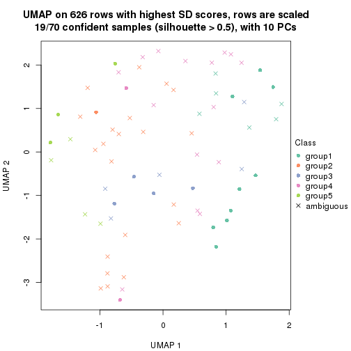
dimension_reduction(res, k = 6, method = "UMAP")
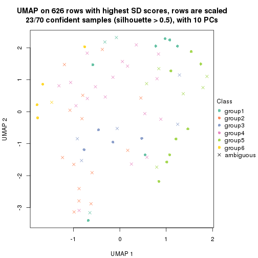
Following heatmap shows how subgroups are split when increasing k:
collect_classes(res)
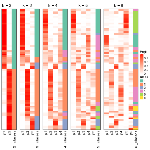
If matrix rows can be associated to genes, consider to use functional_enrichment(res,
...) to perform function enrichment for the signature genes. See this vignette for more detailed explanations.
The object with results only for a single top-value method and a single partition method can be extracted as:
res = res_list["CV", "hclust"]
# you can also extract it by
# res = res_list["CV:hclust"]
A summary of res and all the functions that can be applied to it:
res
#> A 'ConsensusPartition' object with k = 2, 3, 4, 5, 6.
#>   On a matrix with 626 rows and 70 columns.
#>   Top rows (63, 126, 188, 250, 313) are extracted by 'CV' method.
#>   Subgroups are detected by 'hclust' method.
#>   Performed in total 1250 partitions by row resampling.
#>   Best k for subgroups seems to be 3.
#>
#> Following methods can be applied to this 'ConsensusPartition' object:
#>  [1] "cola_report"             "collect_classes"         "collect_plots"
#>  [4] "collect_stats"           "colnames"                "compare_signatures"
#>  [7] "consensus_heatmap"       "dimension_reduction"     "functional_enrichment"
#> [10] "get_anno_col"            "get_anno"                "get_classes"
#> [13] "get_consensus"           "get_matrix"              "get_membership"
#> [16] "get_param"               "get_signatures"          "get_stats"
#> [19] "is_best_k"               "is_stable_k"             "membership_heatmap"
#> [22] "ncol"                    "nrow"                    "plot_ecdf"
#> [25] "rownames"                "select_partition_number" "show"
#> [28] "suggest_best_k"          "test_to_known_factors"
collect_plots() function collects all the plots made from res for all k (number of partitions)
into one single page to provide an easy and fast comparison between different k.
collect_plots(res)
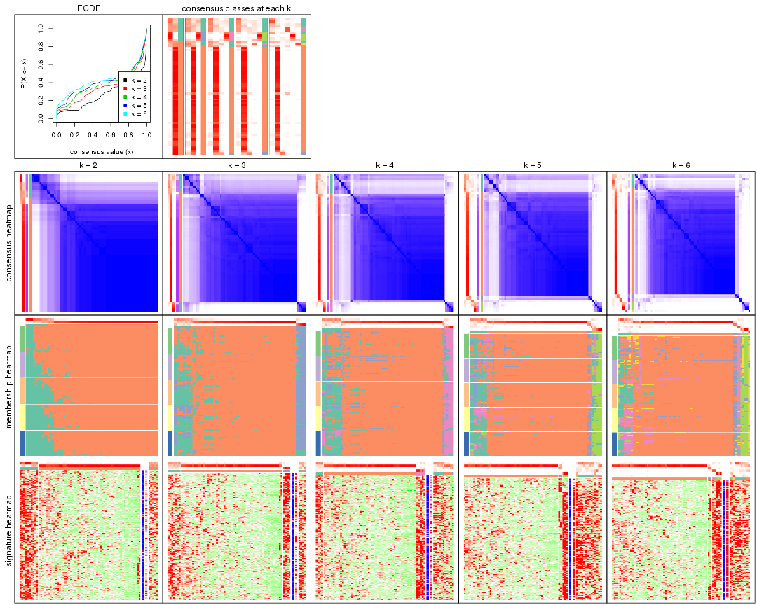
The plots are:
k and the heatmap of
predicted classes for each k.k.k.k.All the plots in panels can be made by individual functions and they are plotted later in this section.
select_partition_number() produces several plots showing different
statistics for choosing “optimized” k. There are following statistics:
k;k, the area increased is defined as \(A_k - A_{k-1}\).The detailed explanations of these statistics can be found in the cola vignette.
Generally speaking, lower PAC score, higher mean silhouette score or higher
concordance corresponds to better partition. Rand index and Jaccard index
measure how similar the current partition is compared to partition with k-1.
If they are too similar, we won't accept k is better than k-1.
select_partition_number(res)
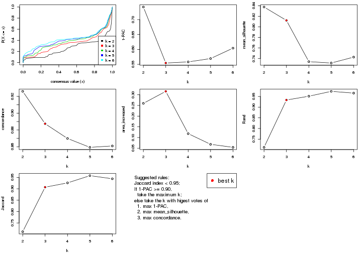
The numeric values for all these statistics can be obtained by get_stats().
get_stats(res)
#>   k 1-PAC mean_silhouette concordance area_increased  Rand Jaccard
#> 2 2 0.742           0.838       0.926         0.2597 0.712   0.712
#> 3 3 0.554           0.812       0.887         0.3159 0.933   0.907
#> 4 4 0.558           0.734       0.870         0.1181 0.951   0.926
#> 5 5 0.569           0.732       0.859         0.0682 0.974   0.958
#> 6 6 0.604           0.743       0.861         0.0541 0.966   0.944
suggest_best_k() suggests the best \(k\) based on these statistics. The rules are as follows:
suggest_best_k(res)
#> [1] 3
Following shows the table of the partitions (You need to click the show/hide
code output link to see it). The membership matrix (columns with name p*)
is inferred by
clue::cl_consensus()
function with the SE method. Basically the value in the membership matrix
represents the probability to belong to a certain group. The finall class
label for an item is determined with the group with highest probability it
belongs to.
In get_classes() function, the entropy is calculated from the membership
matrix and the silhouette score is calculated from the consensus matrix.
cbind(get_classes(res, k = 2), get_membership(res, k = 2))
#>           class entropy silhouette    p1    p2
#> SRR837437     2  0.0000     0.9483 0.000 1.000
#> SRR837438     2  0.4161     0.8658 0.084 0.916
#> SRR837439     2  0.0000     0.9483 0.000 1.000
#> SRR837440     2  0.0000     0.9483 0.000 1.000
#> SRR837441     2  0.0000     0.9483 0.000 1.000
#> SRR837442     2  0.0000     0.9483 0.000 1.000
#> SRR837443     2  0.0000     0.9483 0.000 1.000
#> SRR837444     2  0.0938     0.9429 0.012 0.988
#> SRR837445     2  0.0938     0.9432 0.012 0.988
#> SRR837446     2  0.0000     0.9483 0.000 1.000
#> SRR837447     1  0.9087     0.7018 0.676 0.324
#> SRR837448     1  0.0000     0.6972 1.000 0.000
#> SRR837449     2  0.9970    -0.3444 0.468 0.532
#> SRR837450     1  0.0000     0.6972 1.000 0.000
#> SRR837451     2  0.0000     0.9483 0.000 1.000
#> SRR837452     2  0.0376     0.9471 0.004 0.996
#> SRR837453     2  0.0000     0.9483 0.000 1.000
#> SRR837454     2  0.0000     0.9483 0.000 1.000
#> SRR837455     1  0.8555     0.7312 0.720 0.280
#> SRR837456     1  0.8555     0.7312 0.720 0.280
#> SRR837457     2  0.0000     0.9483 0.000 1.000
#> SRR837458     1  0.1843     0.7063 0.972 0.028
#> SRR837459     2  0.0000     0.9483 0.000 1.000
#> SRR837460     2  0.0000     0.9483 0.000 1.000
#> SRR837461     2  0.0000     0.9483 0.000 1.000
#> SRR837462     2  0.0938     0.9430 0.012 0.988
#> SRR837463     2  0.1633     0.9329 0.024 0.976
#> SRR837464     2  0.0376     0.9470 0.004 0.996
#> SRR837465     2  0.0938     0.9427 0.012 0.988
#> SRR837466     1  0.0376     0.6990 0.996 0.004
#> SRR837467     2  0.0000     0.9483 0.000 1.000
#> SRR837468     2  0.4161     0.8621 0.084 0.916
#> SRR837469     1  0.9983     0.4676 0.524 0.476
#> SRR837470     1  0.9954     0.5058 0.540 0.460
#> SRR837471     2  0.0376     0.9470 0.004 0.996
#> SRR837472     2  0.0000     0.9483 0.000 1.000
#> SRR837473     2  0.2948     0.9055 0.052 0.948
#> SRR837474     2  0.0000     0.9483 0.000 1.000
#> SRR837475     2  0.0000     0.9483 0.000 1.000
#> SRR837476     2  0.0000     0.9483 0.000 1.000
#> SRR837477     2  0.0376     0.9470 0.004 0.996
#> SRR837478     2  0.0376     0.9470 0.004 0.996
#> SRR837479     2  0.0000     0.9483 0.000 1.000
#> SRR837480     2  0.0376     0.9470 0.004 0.996
#> SRR837481     2  0.0376     0.9470 0.004 0.996
#> SRR837482     2  0.0376     0.9470 0.004 0.996
#> SRR837483     1  0.8144     0.7318 0.748 0.252
#> SRR837484     2  0.0000     0.9483 0.000 1.000
#> SRR837485     2  0.0000     0.9483 0.000 1.000
#> SRR837486     2  0.4298     0.8600 0.088 0.912
#> SRR837487     2  0.0000     0.9483 0.000 1.000
#> SRR837488     2  0.0000     0.9483 0.000 1.000
#> SRR837489     2  0.1633     0.9324 0.024 0.976
#> SRR837490     2  0.0938     0.9423 0.012 0.988
#> SRR837491     2  0.3584     0.8872 0.068 0.932
#> SRR837492     2  0.3584     0.8881 0.068 0.932
#> SRR837493     2  0.4022     0.8727 0.080 0.920
#> SRR837494     2  0.0000     0.9483 0.000 1.000
#> SRR837495     2  0.1184     0.9405 0.016 0.984
#> SRR837496     1  0.9833     0.5751 0.576 0.424
#> SRR837497     2  0.9732    -0.0662 0.404 0.596
#> SRR837498     2  0.9608     0.0187 0.384 0.616
#> SRR837499     2  0.4939     0.8338 0.108 0.892
#> SRR837500     2  0.4939     0.8338 0.108 0.892
#> SRR837501     2  0.0000     0.9483 0.000 1.000
#> SRR837502     2  0.0938     0.9426 0.012 0.988
#> SRR837503     1  0.9996     0.4342 0.512 0.488
#> SRR837504     2  0.0000     0.9483 0.000 1.000
#> SRR837505     2  0.0000     0.9483 0.000 1.000
#> SRR837506     2  0.0000     0.9483 0.000 1.000
cbind(get_classes(res, k = 3), get_membership(res, k = 3))
#>           class entropy silhouette    p1    p2    p3
#> SRR837437     2  0.0000      0.926 0.000 1.000 0.000
#> SRR837438     2  0.3267      0.822 0.116 0.884 0.000
#> SRR837439     2  0.0000      0.926 0.000 1.000 0.000
#> SRR837440     2  0.0000      0.926 0.000 1.000 0.000
#> SRR837441     2  0.0000      0.926 0.000 1.000 0.000
#> SRR837442     2  0.0000      0.926 0.000 1.000 0.000
#> SRR837443     2  0.0000      0.926 0.000 1.000 0.000
#> SRR837444     2  0.0829      0.925 0.012 0.984 0.004
#> SRR837445     2  0.0747      0.923 0.016 0.984 0.000
#> SRR837446     2  0.0592      0.923 0.012 0.988 0.000
#> SRR837447     1  0.9083      0.556 0.548 0.196 0.256
#> SRR837448     3  0.0237      0.847 0.004 0.000 0.996
#> SRR837449     1  0.8876      0.637 0.468 0.412 0.120
#> SRR837450     3  0.0237      0.847 0.004 0.000 0.996
#> SRR837451     2  0.0000      0.926 0.000 1.000 0.000
#> SRR837452     2  0.0424      0.925 0.008 0.992 0.000
#> SRR837453     2  0.0000      0.926 0.000 1.000 0.000
#> SRR837454     2  0.0000      0.926 0.000 1.000 0.000
#> SRR837455     1  0.9202      0.295 0.460 0.152 0.388
#> SRR837456     1  0.9202      0.295 0.460 0.152 0.388
#> SRR837457     2  0.0237      0.926 0.004 0.996 0.000
#> SRR837458     3  0.3715      0.810 0.128 0.004 0.868
#> SRR837459     2  0.0000      0.926 0.000 1.000 0.000
#> SRR837460     2  0.0237      0.926 0.004 0.996 0.000
#> SRR837461     2  0.0592      0.925 0.012 0.988 0.000
#> SRR837462     2  0.1529      0.915 0.040 0.960 0.000
#> SRR837463     2  0.1964      0.905 0.056 0.944 0.000
#> SRR837464     2  0.1411      0.916 0.036 0.964 0.000
#> SRR837465     2  0.1031      0.922 0.024 0.976 0.000
#> SRR837466     3  0.1964      0.844 0.056 0.000 0.944
#> SRR837467     2  0.0237      0.926 0.004 0.996 0.000
#> SRR837468     2  0.5315      0.618 0.216 0.772 0.012
#> SRR837469     1  0.8698      0.695 0.564 0.300 0.136
#> SRR837470     1  0.8825      0.692 0.560 0.288 0.152
#> SRR837471     2  0.0237      0.926 0.004 0.996 0.000
#> SRR837472     2  0.0000      0.926 0.000 1.000 0.000
#> SRR837473     2  0.3454      0.825 0.104 0.888 0.008
#> SRR837474     2  0.0000      0.926 0.000 1.000 0.000
#> SRR837475     2  0.0592      0.924 0.012 0.988 0.000
#> SRR837476     2  0.0000      0.926 0.000 1.000 0.000
#> SRR837477     2  0.0892      0.924 0.020 0.980 0.000
#> SRR837478     2  0.1031      0.923 0.024 0.976 0.000
#> SRR837479     2  0.1031      0.922 0.024 0.976 0.000
#> SRR837480     2  0.0892      0.924 0.020 0.980 0.000
#> SRR837481     2  0.1411      0.917 0.036 0.964 0.000
#> SRR837482     2  0.1289      0.919 0.032 0.968 0.000
#> SRR837483     3  0.8138      0.285 0.232 0.132 0.636
#> SRR837484     2  0.1529      0.915 0.040 0.960 0.000
#> SRR837485     2  0.1411      0.917 0.036 0.964 0.000
#> SRR837486     2  0.4873      0.736 0.152 0.824 0.024
#> SRR837487     2  0.0237      0.926 0.004 0.996 0.000
#> SRR837488     2  0.0237      0.926 0.004 0.996 0.000
#> SRR837489     2  0.1753      0.898 0.048 0.952 0.000
#> SRR837490     2  0.1411      0.910 0.036 0.964 0.000
#> SRR837491     2  0.3038      0.839 0.104 0.896 0.000
#> SRR837492     2  0.4345      0.770 0.136 0.848 0.016
#> SRR837493     2  0.3267      0.824 0.116 0.884 0.000
#> SRR837494     2  0.0000      0.926 0.000 1.000 0.000
#> SRR837495     2  0.1267      0.920 0.024 0.972 0.004
#> SRR837496     1  0.9431      0.676 0.500 0.280 0.220
#> SRR837497     1  0.6819      0.621 0.644 0.328 0.028
#> SRR837498     2  0.7581     -0.474 0.464 0.496 0.040
#> SRR837499     2  0.4047      0.770 0.148 0.848 0.004
#> SRR837500     2  0.4047      0.770 0.148 0.848 0.004
#> SRR837501     2  0.5098      0.576 0.248 0.752 0.000
#> SRR837502     2  0.1031      0.918 0.024 0.976 0.000
#> SRR837503     1  0.9507      0.661 0.432 0.380 0.188
#> SRR837504     2  0.0237      0.926 0.004 0.996 0.000
#> SRR837505     2  0.2796      0.853 0.092 0.908 0.000
#> SRR837506     2  0.5363      0.520 0.276 0.724 0.000
cbind(get_classes(res, k = 4), get_membership(res, k = 4))
#>           class entropy silhouette    p1    p2    p3    p4
#> SRR837437     2  0.0188     0.8955 0.000 0.996 0.004 0.000
#> SRR837438     2  0.2888     0.7179 0.124 0.872 0.004 0.000
#> SRR837439     2  0.0188     0.8955 0.000 0.996 0.004 0.000
#> SRR837440     2  0.0188     0.8955 0.000 0.996 0.004 0.000
#> SRR837441     2  0.0188     0.8955 0.000 0.996 0.004 0.000
#> SRR837442     2  0.0188     0.8955 0.000 0.996 0.004 0.000
#> SRR837443     2  0.0188     0.8955 0.000 0.996 0.004 0.000
#> SRR837444     2  0.0672     0.8941 0.008 0.984 0.008 0.000
#> SRR837445     2  0.0779     0.8901 0.016 0.980 0.004 0.000
#> SRR837446     2  0.0469     0.8905 0.000 0.988 0.012 0.000
#> SRR837447     1  0.6528     0.5480 0.692 0.168 0.032 0.108
#> SRR837448     4  0.0469     0.8379 0.012 0.000 0.000 0.988
#> SRR837449     1  0.6592     0.3434 0.556 0.380 0.028 0.036
#> SRR837450     4  0.0469     0.8379 0.012 0.000 0.000 0.988
#> SRR837451     2  0.0188     0.8955 0.000 0.996 0.004 0.000
#> SRR837452     2  0.0336     0.8944 0.008 0.992 0.000 0.000
#> SRR837453     2  0.0188     0.8955 0.000 0.996 0.004 0.000
#> SRR837454     2  0.0188     0.8955 0.000 0.996 0.004 0.000
#> SRR837455     1  0.7872     0.3387 0.608 0.124 0.100 0.168
#> SRR837456     1  0.7872     0.3387 0.608 0.124 0.100 0.168
#> SRR837457     2  0.0336     0.8953 0.000 0.992 0.008 0.000
#> SRR837458     4  0.6134     0.7372 0.216 0.000 0.116 0.668
#> SRR837459     2  0.0188     0.8955 0.000 0.996 0.004 0.000
#> SRR837460     2  0.0336     0.8953 0.000 0.992 0.008 0.000
#> SRR837461     2  0.0657     0.8943 0.004 0.984 0.012 0.000
#> SRR837462     2  0.1724     0.8651 0.020 0.948 0.032 0.000
#> SRR837463     2  0.2032     0.8549 0.036 0.936 0.028 0.000
#> SRR837464     2  0.1488     0.8711 0.012 0.956 0.032 0.000
#> SRR837465     2  0.0927     0.8887 0.016 0.976 0.008 0.000
#> SRR837466     4  0.3056     0.8331 0.072 0.000 0.040 0.888
#> SRR837467     2  0.0188     0.8951 0.004 0.996 0.000 0.000
#> SRR837468     2  0.5744     0.0938 0.184 0.708 0.108 0.000
#> SRR837469     1  0.7398     0.5730 0.608 0.208 0.152 0.032
#> SRR837470     1  0.7535     0.5638 0.608 0.200 0.148 0.044
#> SRR837471     2  0.0336     0.8955 0.000 0.992 0.008 0.000
#> SRR837472     2  0.0188     0.8955 0.000 0.996 0.004 0.000
#> SRR837473     2  0.3670     0.6923 0.100 0.860 0.032 0.008
#> SRR837474     2  0.0188     0.8955 0.000 0.996 0.004 0.000
#> SRR837475     2  0.0937     0.8887 0.012 0.976 0.012 0.000
#> SRR837476     2  0.0000     0.8943 0.000 1.000 0.000 0.000
#> SRR837477     2  0.1059     0.8881 0.016 0.972 0.012 0.000
#> SRR837478     2  0.1182     0.8852 0.016 0.968 0.016 0.000
#> SRR837479     2  0.1406     0.8769 0.016 0.960 0.024 0.000
#> SRR837480     2  0.0927     0.8899 0.008 0.976 0.016 0.000
#> SRR837481     2  0.1520     0.8752 0.020 0.956 0.024 0.000
#> SRR837482     2  0.1411     0.8782 0.020 0.960 0.020 0.000
#> SRR837483     4  0.7865     0.6102 0.228 0.028 0.200 0.544
#> SRR837484     2  0.1733     0.8664 0.028 0.948 0.024 0.000
#> SRR837485     2  0.1510     0.8743 0.016 0.956 0.028 0.000
#> SRR837486     2  0.4992     0.4900 0.104 0.788 0.100 0.008
#> SRR837487     2  0.0376     0.8957 0.004 0.992 0.004 0.000
#> SRR837488     2  0.0376     0.8957 0.004 0.992 0.004 0.000
#> SRR837489     2  0.1474     0.8493 0.052 0.948 0.000 0.000
#> SRR837490     2  0.1305     0.8687 0.036 0.960 0.004 0.000
#> SRR837491     2  0.2799     0.7442 0.108 0.884 0.008 0.000
#> SRR837492     2  0.5172     0.4342 0.136 0.776 0.076 0.012
#> SRR837493     2  0.2976     0.7200 0.120 0.872 0.008 0.000
#> SRR837494     2  0.0188     0.8955 0.000 0.996 0.004 0.000
#> SRR837495     2  0.1182     0.8845 0.016 0.968 0.016 0.000
#> SRR837496     1  0.7529     0.5804 0.624 0.200 0.084 0.092
#> SRR837497     1  0.7720     0.3322 0.476 0.164 0.348 0.012
#> SRR837498     1  0.5833     0.1389 0.528 0.440 0.032 0.000
#> SRR837499     2  0.3529     0.6362 0.152 0.836 0.012 0.000
#> SRR837500     2  0.3529     0.6362 0.152 0.836 0.012 0.000
#> SRR837501     2  0.4843    -0.7166 0.000 0.604 0.396 0.000
#> SRR837502     2  0.1174     0.8829 0.020 0.968 0.012 0.000
#> SRR837503     1  0.7671     0.4709 0.536 0.328 0.056 0.080
#> SRR837504     2  0.0336     0.8953 0.000 0.992 0.008 0.000
#> SRR837505     2  0.2773     0.7044 0.004 0.880 0.116 0.000
#> SRR837506     3  0.5000     0.0000 0.000 0.500 0.500 0.000
cbind(get_classes(res, k = 5), get_membership(res, k = 5))
#>           class entropy silhouette    p1    p2    p3    p4    p5
#> SRR837437     2  0.0162     0.9152 0.000 0.996 0.004 0.000 0.000
#> SRR837438     2  0.2733     0.7723 0.112 0.872 0.004 0.012 0.000
#> SRR837439     2  0.0162     0.9152 0.000 0.996 0.004 0.000 0.000
#> SRR837440     2  0.0162     0.9152 0.000 0.996 0.004 0.000 0.000
#> SRR837441     2  0.0162     0.9152 0.000 0.996 0.004 0.000 0.000
#> SRR837442     2  0.0162     0.9152 0.000 0.996 0.004 0.000 0.000
#> SRR837443     2  0.0162     0.9152 0.000 0.996 0.004 0.000 0.000
#> SRR837444     2  0.0579     0.9143 0.008 0.984 0.000 0.008 0.000
#> SRR837445     2  0.0693     0.9112 0.012 0.980 0.000 0.008 0.000
#> SRR837446     2  0.0451     0.9118 0.000 0.988 0.008 0.004 0.000
#> SRR837447     1  0.5007     0.3365 0.752 0.148 0.016 0.012 0.072
#> SRR837448     5  0.0000     0.6922 0.000 0.000 0.000 0.000 1.000
#> SRR837449     1  0.6010     0.2420 0.552 0.372 0.012 0.040 0.024
#> SRR837450     5  0.0000     0.6922 0.000 0.000 0.000 0.000 1.000
#> SRR837451     2  0.0162     0.9152 0.000 0.996 0.004 0.000 0.000
#> SRR837452     2  0.0324     0.9144 0.004 0.992 0.000 0.004 0.000
#> SRR837453     2  0.0162     0.9152 0.000 0.996 0.004 0.000 0.000
#> SRR837454     2  0.0162     0.9152 0.000 0.996 0.004 0.000 0.000
#> SRR837455     1  0.7343     0.1758 0.608 0.112 0.088 0.148 0.044
#> SRR837456     1  0.7343     0.1758 0.608 0.112 0.088 0.148 0.044
#> SRR837457     2  0.0324     0.9152 0.000 0.992 0.004 0.004 0.000
#> SRR837458     5  0.7984     0.4538 0.220 0.000 0.140 0.192 0.448
#> SRR837459     2  0.0162     0.9152 0.000 0.996 0.004 0.000 0.000
#> SRR837460     2  0.0451     0.9146 0.004 0.988 0.008 0.000 0.000
#> SRR837461     2  0.0727     0.9134 0.004 0.980 0.012 0.004 0.000
#> SRR837462     2  0.1893     0.8787 0.024 0.936 0.028 0.012 0.000
#> SRR837463     2  0.2104     0.8706 0.044 0.924 0.024 0.008 0.000
#> SRR837464     2  0.1686     0.8850 0.020 0.944 0.028 0.008 0.000
#> SRR837465     2  0.0960     0.9088 0.016 0.972 0.008 0.004 0.000
#> SRR837466     5  0.4488     0.6815 0.088 0.000 0.072 0.044 0.796
#> SRR837467     2  0.0162     0.9150 0.000 0.996 0.000 0.004 0.000
#> SRR837468     2  0.6050    -0.0289 0.156 0.640 0.180 0.024 0.000
#> SRR837469     1  0.7588     0.0773 0.540 0.120 0.208 0.120 0.012
#> SRR837470     1  0.7600     0.0562 0.552 0.112 0.200 0.116 0.020
#> SRR837471     2  0.0324     0.9152 0.000 0.992 0.004 0.004 0.000
#> SRR837472     2  0.0162     0.9152 0.000 0.996 0.004 0.000 0.000
#> SRR837473     2  0.3418     0.7345 0.084 0.852 0.004 0.056 0.004
#> SRR837474     2  0.0162     0.9152 0.000 0.996 0.004 0.000 0.000
#> SRR837475     2  0.0968     0.9075 0.012 0.972 0.004 0.012 0.000
#> SRR837476     2  0.0000     0.9143 0.000 1.000 0.000 0.000 0.000
#> SRR837477     2  0.1087     0.9071 0.008 0.968 0.008 0.016 0.000
#> SRR837478     2  0.1200     0.9047 0.008 0.964 0.012 0.016 0.000
#> SRR837479     2  0.1393     0.8982 0.008 0.956 0.024 0.012 0.000
#> SRR837480     2  0.0960     0.9091 0.004 0.972 0.008 0.016 0.000
#> SRR837481     2  0.1597     0.8933 0.024 0.948 0.020 0.008 0.000
#> SRR837482     2  0.1471     0.8960 0.024 0.952 0.020 0.004 0.000
#> SRR837483     5  0.6588     0.3542 0.088 0.000 0.040 0.384 0.488
#> SRR837484     2  0.1854     0.8806 0.036 0.936 0.020 0.008 0.000
#> SRR837485     2  0.1471     0.8953 0.020 0.952 0.024 0.004 0.000
#> SRR837486     2  0.5143     0.4995 0.060 0.756 0.048 0.128 0.008
#> SRR837487     2  0.0324     0.9154 0.004 0.992 0.004 0.000 0.000
#> SRR837488     2  0.0324     0.9154 0.004 0.992 0.004 0.000 0.000
#> SRR837489     2  0.1408     0.8795 0.044 0.948 0.000 0.008 0.000
#> SRR837490     2  0.1243     0.8943 0.028 0.960 0.004 0.008 0.000
#> SRR837491     2  0.2623     0.7931 0.096 0.884 0.004 0.016 0.000
#> SRR837492     2  0.4702     0.5061 0.112 0.764 0.004 0.112 0.008
#> SRR837493     2  0.2784     0.7734 0.108 0.872 0.004 0.016 0.000
#> SRR837494     2  0.0162     0.9152 0.000 0.996 0.004 0.000 0.000
#> SRR837495     2  0.1012     0.9070 0.012 0.968 0.000 0.020 0.000
#> SRR837496     1  0.7238     0.2714 0.564 0.168 0.008 0.188 0.072
#> SRR837497     4  0.4843     0.0000 0.204 0.048 0.020 0.728 0.000
#> SRR837498     1  0.6451     0.1421 0.500 0.388 0.028 0.080 0.004
#> SRR837499     2  0.3264     0.7051 0.140 0.836 0.004 0.020 0.000
#> SRR837500     2  0.3264     0.7051 0.140 0.836 0.004 0.020 0.000
#> SRR837501     3  0.4744     0.6730 0.000 0.476 0.508 0.016 0.000
#> SRR837502     2  0.1278     0.9000 0.016 0.960 0.004 0.020 0.000
#> SRR837503     1  0.7123     0.3914 0.504 0.304 0.000 0.128 0.064
#> SRR837504     2  0.0324     0.9152 0.000 0.992 0.004 0.004 0.000
#> SRR837505     2  0.2942     0.7219 0.008 0.856 0.128 0.008 0.000
#> SRR837506     3  0.4555     0.6165 0.000 0.344 0.636 0.020 0.000
cbind(get_classes(res, k = 6), get_membership(res, k = 6))
#>           class entropy silhouette    p1    p2    p3    p4    p5    p6
#> SRR837437     2  0.0146     0.9158 0.000 0.996 0.004 0.000 0.000 0.000
#> SRR837438     2  0.2862     0.8174 0.056 0.872 0.000 0.052 0.000 0.020
#> SRR837439     2  0.0146     0.9158 0.000 0.996 0.004 0.000 0.000 0.000
#> SRR837440     2  0.0146     0.9158 0.000 0.996 0.004 0.000 0.000 0.000
#> SRR837441     2  0.0146     0.9158 0.000 0.996 0.004 0.000 0.000 0.000
#> SRR837442     2  0.0146     0.9158 0.000 0.996 0.004 0.000 0.000 0.000
#> SRR837443     2  0.0146     0.9158 0.000 0.996 0.004 0.000 0.000 0.000
#> SRR837444     2  0.0508     0.9156 0.000 0.984 0.004 0.012 0.000 0.000
#> SRR837445     2  0.0665     0.9135 0.004 0.980 0.000 0.008 0.000 0.008
#> SRR837446     2  0.0405     0.9138 0.000 0.988 0.008 0.004 0.000 0.000
#> SRR837447     1  0.6884     0.2780 0.580 0.132 0.012 0.180 0.060 0.036
#> SRR837448     5  0.0000     0.6914 0.000 0.000 0.000 0.000 1.000 0.000
#> SRR837449     1  0.7512     0.1696 0.400 0.364 0.024 0.120 0.020 0.072
#> SRR837450     5  0.0000     0.6914 0.000 0.000 0.000 0.000 1.000 0.000
#> SRR837451     2  0.0146     0.9158 0.000 0.996 0.004 0.000 0.000 0.000
#> SRR837452     2  0.0291     0.9155 0.004 0.992 0.000 0.000 0.000 0.004
#> SRR837453     2  0.0146     0.9158 0.000 0.996 0.004 0.000 0.000 0.000
#> SRR837454     2  0.0146     0.9158 0.000 0.996 0.004 0.000 0.000 0.000
#> SRR837455     1  0.3462     0.2900 0.840 0.100 0.016 0.028 0.008 0.008
#> SRR837456     1  0.3462     0.2900 0.840 0.100 0.016 0.028 0.008 0.008
#> SRR837457     2  0.0260     0.9161 0.000 0.992 0.008 0.000 0.000 0.000
#> SRR837458     1  0.7141    -0.4870 0.492 0.000 0.136 0.060 0.268 0.044
#> SRR837459     2  0.0146     0.9158 0.000 0.996 0.004 0.000 0.000 0.000
#> SRR837460     2  0.0520     0.9147 0.000 0.984 0.008 0.008 0.000 0.000
#> SRR837461     2  0.0717     0.9136 0.000 0.976 0.008 0.016 0.000 0.000
#> SRR837462     2  0.1644     0.8878 0.000 0.932 0.028 0.040 0.000 0.000
#> SRR837463     2  0.1989     0.8785 0.004 0.916 0.028 0.052 0.000 0.000
#> SRR837464     2  0.1575     0.8895 0.000 0.936 0.032 0.032 0.000 0.000
#> SRR837465     2  0.0806     0.9119 0.000 0.972 0.008 0.020 0.000 0.000
#> SRR837466     5  0.5872     0.5914 0.144 0.000 0.112 0.048 0.664 0.032
#> SRR837467     2  0.0146     0.9158 0.000 0.996 0.000 0.000 0.000 0.004
#> SRR837468     2  0.5029     0.0274 0.016 0.568 0.048 0.368 0.000 0.000
#> SRR837469     4  0.2957     0.9486 0.120 0.032 0.000 0.844 0.004 0.000
#> SRR837470     4  0.3225     0.9483 0.136 0.024 0.000 0.828 0.008 0.004
#> SRR837471     2  0.0291     0.9159 0.000 0.992 0.004 0.000 0.000 0.004
#> SRR837472     2  0.0146     0.9158 0.000 0.996 0.004 0.000 0.000 0.000
#> SRR837473     2  0.3458     0.7764 0.084 0.840 0.016 0.012 0.000 0.048
#> SRR837474     2  0.0146     0.9158 0.000 0.996 0.004 0.000 0.000 0.000
#> SRR837475     2  0.0951     0.9095 0.020 0.968 0.004 0.000 0.000 0.008
#> SRR837476     2  0.0000     0.9151 0.000 1.000 0.000 0.000 0.000 0.000
#> SRR837477     2  0.1235     0.9066 0.008 0.960 0.008 0.016 0.000 0.008
#> SRR837478     2  0.1337     0.9047 0.008 0.956 0.012 0.016 0.000 0.008
#> SRR837479     2  0.1553     0.8964 0.008 0.944 0.032 0.012 0.000 0.004
#> SRR837480     2  0.1026     0.9105 0.004 0.968 0.012 0.008 0.000 0.008
#> SRR837481     2  0.1578     0.8996 0.012 0.944 0.012 0.028 0.000 0.004
#> SRR837482     2  0.1332     0.9035 0.008 0.952 0.012 0.028 0.000 0.000
#> SRR837483     5  0.7773     0.2607 0.120 0.000 0.080 0.088 0.424 0.288
#> SRR837484     2  0.1766     0.8932 0.016 0.936 0.016 0.028 0.000 0.004
#> SRR837485     2  0.1350     0.9030 0.008 0.952 0.020 0.020 0.000 0.000
#> SRR837486     2  0.5019     0.6266 0.040 0.748 0.044 0.088 0.000 0.080
#> SRR837487     2  0.0291     0.9161 0.004 0.992 0.004 0.000 0.000 0.000
#> SRR837488     2  0.0291     0.9161 0.004 0.992 0.004 0.000 0.000 0.000
#> SRR837489     2  0.1570     0.8907 0.028 0.944 0.004 0.008 0.000 0.016
#> SRR837490     2  0.1173     0.9021 0.016 0.960 0.000 0.008 0.000 0.016
#> SRR837491     2  0.2688     0.8316 0.044 0.884 0.000 0.048 0.000 0.024
#> SRR837492     2  0.4721     0.6204 0.116 0.752 0.024 0.020 0.000 0.088
#> SRR837493     2  0.2880     0.8181 0.056 0.872 0.000 0.048 0.000 0.024
#> SRR837494     2  0.0146     0.9158 0.000 0.996 0.004 0.000 0.000 0.000
#> SRR837495     2  0.1007     0.9109 0.004 0.968 0.004 0.016 0.000 0.008
#> SRR837496     1  0.8641     0.2729 0.392 0.144 0.032 0.164 0.060 0.208
#> SRR837497     6  0.2781     0.0000 0.048 0.008 0.004 0.064 0.000 0.876
#> SRR837498     2  0.7602    -0.5413 0.264 0.360 0.016 0.264 0.000 0.096
#> SRR837499     2  0.3478     0.7714 0.084 0.836 0.004 0.052 0.000 0.024
#> SRR837500     2  0.3478     0.7714 0.084 0.836 0.004 0.052 0.000 0.024
#> SRR837501     3  0.3405     0.7244 0.000 0.272 0.724 0.004 0.000 0.000
#> SRR837502     2  0.1312     0.9038 0.008 0.956 0.012 0.004 0.000 0.020
#> SRR837503     1  0.8479     0.2899 0.368 0.288 0.032 0.116 0.052 0.144
#> SRR837504     2  0.0260     0.9161 0.000 0.992 0.008 0.000 0.000 0.000
#> SRR837505     2  0.2945     0.7386 0.000 0.824 0.156 0.020 0.000 0.000
#> SRR837506     3  0.5348     0.6717 0.004 0.188 0.676 0.076 0.000 0.056
Heatmaps for the consensus matrix. It visualizes the probability of two samples to be in a same group.
consensus_heatmap(res, k = 2)
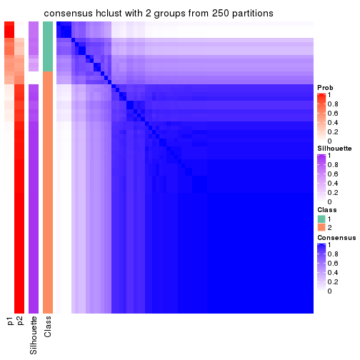
consensus_heatmap(res, k = 3)
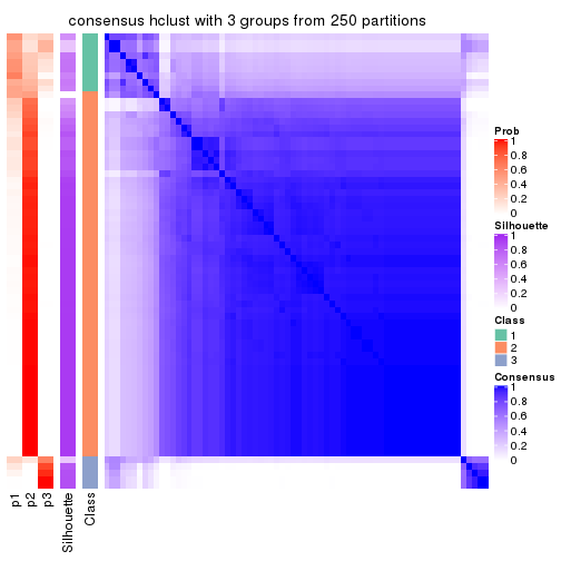
consensus_heatmap(res, k = 4)
consensus_heatmap(res, k = 5)
consensus_heatmap(res, k = 6)
Heatmaps for the membership of samples in all partitions to see how consistent they are:
membership_heatmap(res, k = 2)
membership_heatmap(res, k = 3)
membership_heatmap(res, k = 4)
membership_heatmap(res, k = 5)
membership_heatmap(res, k = 6)
As soon as we have had the classes for columns, we can look for signatures which are significantly different between classes which can be candidate marks for certain classes. Following are the heatmaps for signatures.
Signature heatmaps where rows are scaled:
get_signatures(res, k = 2)
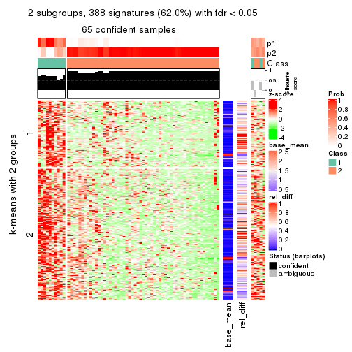
get_signatures(res, k = 3)
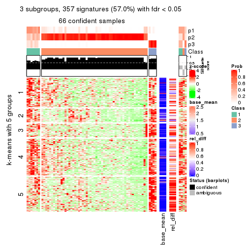
get_signatures(res, k = 4)
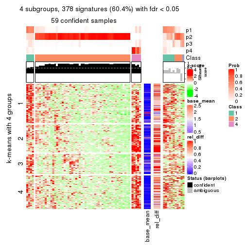
get_signatures(res, k = 5)
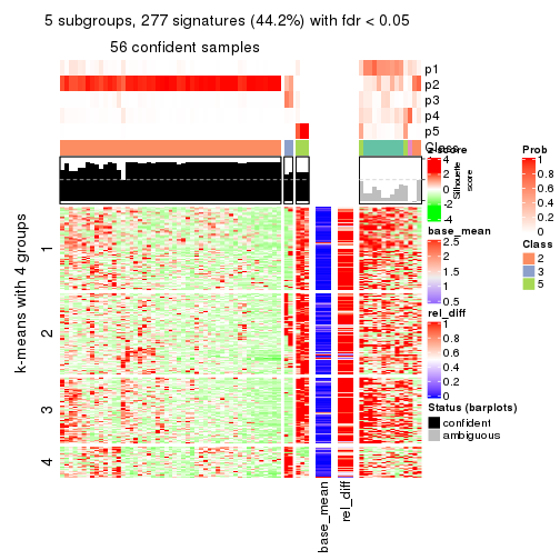
get_signatures(res, k = 6)
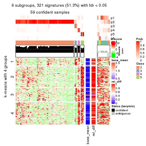
Signature heatmaps where rows are not scaled:
get_signatures(res, k = 2, scale_rows = FALSE)
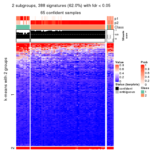
get_signatures(res, k = 3, scale_rows = FALSE)
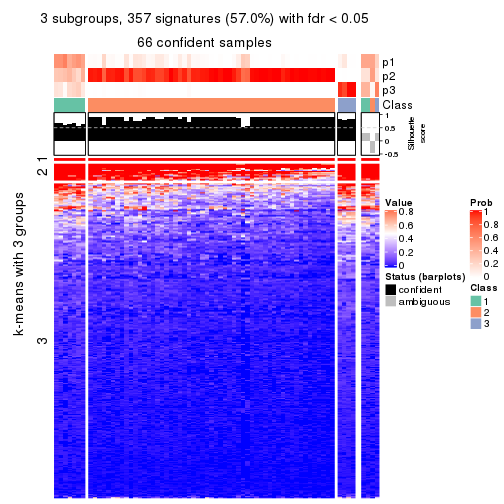
get_signatures(res, k = 4, scale_rows = FALSE)
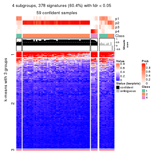
get_signatures(res, k = 5, scale_rows = FALSE)
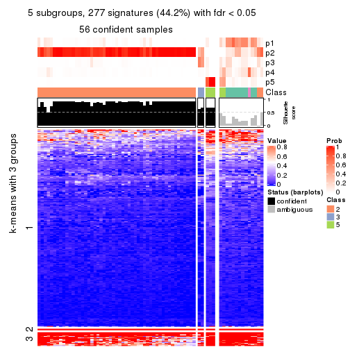
get_signatures(res, k = 6, scale_rows = FALSE)
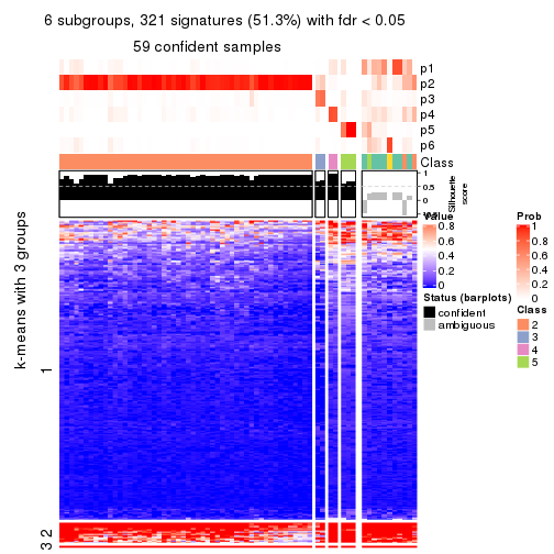
Compare the overlap of signatures from different k:
compare_signatures(res)
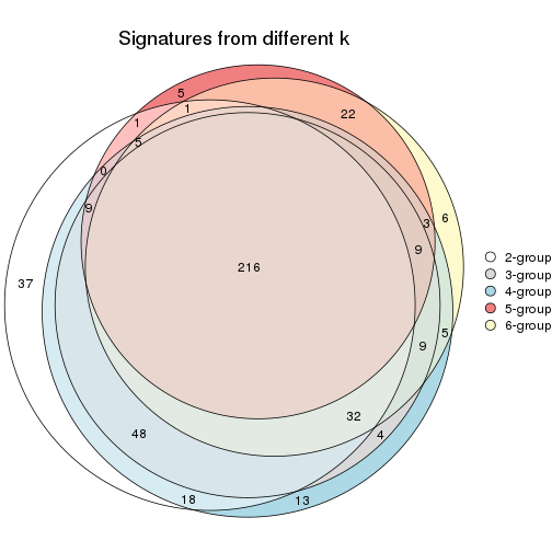
get_signature() returns a data frame invisibly. TO get the list of signatures, the function
call should be assigned to a variable explicitly. In following code, if plot argument is set
to FALSE, no heatmap is plotted while only the differential analysis is performed.
# code only for demonstration
tb = get_signature(res, k = ..., plot = FALSE)
An example of the output of tb is:
#>   which_row         fdr    mean_1    mean_2 scaled_mean_1 scaled_mean_2 km
#> 1        38 0.042760348  8.373488  9.131774    -0.5533452     0.5164555  1
#> 2        40 0.018707592  7.106213  8.469186    -0.6173731     0.5762149  1
#> 3        55 0.019134737 10.221463 11.207825    -0.6159697     0.5749050  1
#> 4        59 0.006059896  5.921854  7.869574    -0.6899429     0.6439467  1
#> 5        60 0.018055526  8.928898 10.211722    -0.6204761     0.5791110  1
#> 6        98 0.009384629 15.714769 14.887706     0.6635654    -0.6193277  2
...
The columns in tb are:
which_row: row indices corresponding to the input matrix.fdr: FDR for the differential test. mean_x: The mean value in group x.scaled_mean_x: The mean value in group x after rows are scaled.km: Row groups if k-means clustering is applied to rows.UMAP plot which shows how samples are separated.
dimension_reduction(res, k = 2, method = "UMAP")
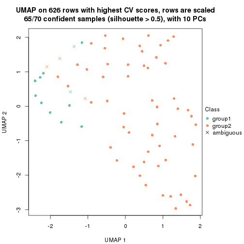
dimension_reduction(res, k = 3, method = "UMAP")

dimension_reduction(res, k = 4, method = "UMAP")
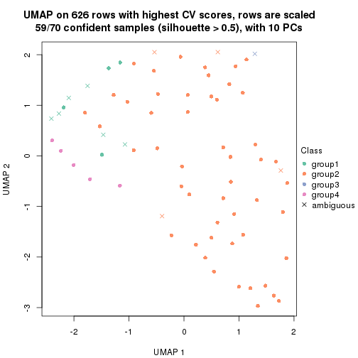
dimension_reduction(res, k = 5, method = "UMAP")
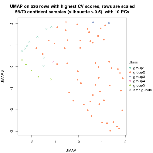
dimension_reduction(res, k = 6, method = "UMAP")
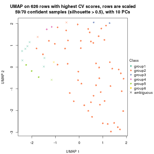
Following heatmap shows how subgroups are split when increasing k:
collect_classes(res)
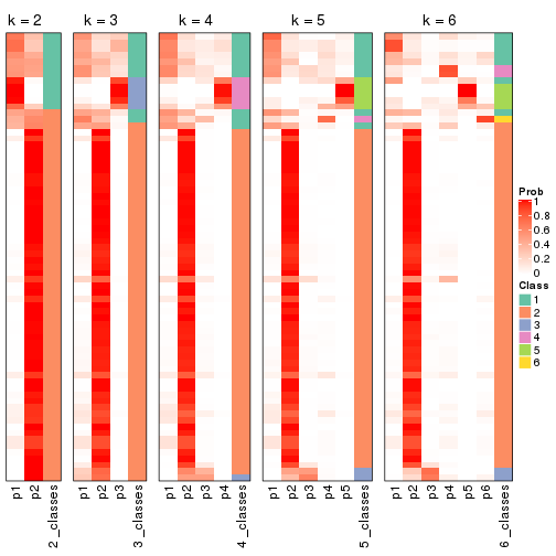
If matrix rows can be associated to genes, consider to use functional_enrichment(res,
...) to perform function enrichment for the signature genes. See this vignette for more detailed explanations.
The object with results only for a single top-value method and a single partition method can be extracted as:
res = res_list["CV", "kmeans"]
# you can also extract it by
# res = res_list["CV:kmeans"]
A summary of res and all the functions that can be applied to it:
res
#> A 'ConsensusPartition' object with k = 2, 3, 4, 5, 6.
#>   On a matrix with 626 rows and 70 columns.
#>   Top rows (63, 126, 188, 250, 313) are extracted by 'CV' method.
#>   Subgroups are detected by 'kmeans' method.
#>   Performed in total 1250 partitions by row resampling.
#>   Best k for subgroups seems to be 3.
#>
#> Following methods can be applied to this 'ConsensusPartition' object:
#>  [1] "cola_report"             "collect_classes"         "collect_plots"
#>  [4] "collect_stats"           "colnames"                "compare_signatures"
#>  [7] "consensus_heatmap"       "dimension_reduction"     "functional_enrichment"
#> [10] "get_anno_col"            "get_anno"                "get_classes"
#> [13] "get_consensus"           "get_matrix"              "get_membership"
#> [16] "get_param"               "get_signatures"          "get_stats"
#> [19] "is_best_k"               "is_stable_k"             "membership_heatmap"
#> [22] "ncol"                    "nrow"                    "plot_ecdf"
#> [25] "rownames"                "select_partition_number" "show"
#> [28] "suggest_best_k"          "test_to_known_factors"
collect_plots() function collects all the plots made from res for all k (number of partitions)
into one single page to provide an easy and fast comparison between different k.
collect_plots(res)
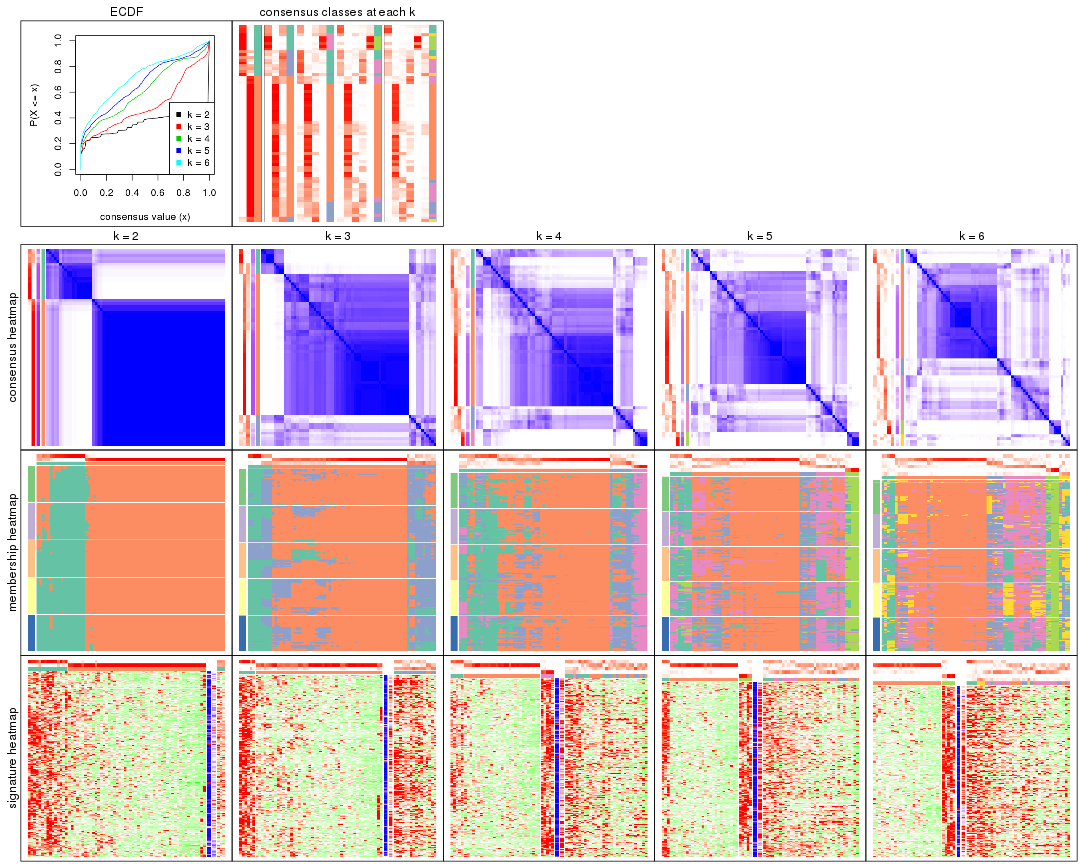
The plots are:
k and the heatmap of
predicted classes for each k.k.k.k.All the plots in panels can be made by individual functions and they are plotted later in this section.
select_partition_number() produces several plots showing different
statistics for choosing “optimized” k. There are following statistics:
k;k, the area increased is defined as \(A_k - A_{k-1}\).The detailed explanations of these statistics can be found in the cola vignette.
Generally speaking, lower PAC score, higher mean silhouette score or higher
concordance corresponds to better partition. Rand index and Jaccard index
measure how similar the current partition is compared to partition with k-1.
If they are too similar, we won't accept k is better than k-1.
select_partition_number(res)
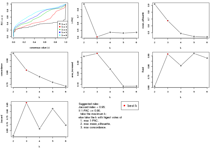
The numeric values for all these statistics can be obtained by get_stats().
get_stats(res)
#>   k 1-PAC mean_silhouette concordance area_increased  Rand Jaccard
#> 2 2 0.881           0.918       0.960         0.3588 0.612   0.612
#> 3 3 0.405           0.676       0.820         0.3857 0.918   0.867
#> 4 4 0.471           0.489       0.765         0.2414 0.807   0.665
#> 5 5 0.460           0.444       0.718         0.0839 0.923   0.821
#> 6 6 0.470           0.439       0.685         0.0846 0.879   0.693
suggest_best_k() suggests the best \(k\) based on these statistics. The rules are as follows:
suggest_best_k(res)
#> [1] 3
Following shows the table of the partitions (You need to click the show/hide
code output link to see it). The membership matrix (columns with name p*)
is inferred by
clue::cl_consensus()
function with the SE method. Basically the value in the membership matrix
represents the probability to belong to a certain group. The finall class
label for an item is determined with the group with highest probability it
belongs to.
In get_classes() function, the entropy is calculated from the membership
matrix and the silhouette score is calculated from the consensus matrix.
cbind(get_classes(res, k = 2), get_membership(res, k = 2))
#>           class entropy silhouette    p1    p2
#> SRR837437     2  0.0000      0.989 0.000 1.000
#> SRR837438     2  0.0000      0.989 0.000 1.000
#> SRR837439     2  0.0000      0.989 0.000 1.000
#> SRR837440     2  0.0000      0.989 0.000 1.000
#> SRR837441     2  0.0000      0.989 0.000 1.000
#> SRR837442     2  0.0000      0.989 0.000 1.000
#> SRR837443     2  0.0000      0.989 0.000 1.000
#> SRR837444     2  0.0000      0.989 0.000 1.000
#> SRR837445     2  0.0000      0.989 0.000 1.000
#> SRR837446     2  0.0000      0.989 0.000 1.000
#> SRR837447     1  0.4022      0.840 0.920 0.080
#> SRR837448     1  0.0000      0.859 1.000 0.000
#> SRR837449     1  0.9393      0.576 0.644 0.356
#> SRR837450     1  0.0000      0.859 1.000 0.000
#> SRR837451     2  0.0000      0.989 0.000 1.000
#> SRR837452     2  0.0000      0.989 0.000 1.000
#> SRR837453     2  0.0000      0.989 0.000 1.000
#> SRR837454     2  0.0000      0.989 0.000 1.000
#> SRR837455     1  0.2236      0.859 0.964 0.036
#> SRR837456     1  0.2043      0.860 0.968 0.032
#> SRR837457     2  0.0000      0.989 0.000 1.000
#> SRR837458     1  0.0000      0.859 1.000 0.000
#> SRR837459     2  0.0000      0.989 0.000 1.000
#> SRR837460     2  0.0000      0.989 0.000 1.000
#> SRR837461     2  0.0000      0.989 0.000 1.000
#> SRR837462     2  0.0000      0.989 0.000 1.000
#> SRR837463     2  0.0000      0.989 0.000 1.000
#> SRR837464     2  0.0000      0.989 0.000 1.000
#> SRR837465     2  0.0000      0.989 0.000 1.000
#> SRR837466     1  0.0000      0.859 1.000 0.000
#> SRR837467     2  0.0000      0.989 0.000 1.000
#> SRR837468     2  0.5842      0.810 0.140 0.860
#> SRR837469     1  0.1184      0.861 0.984 0.016
#> SRR837470     1  0.0000      0.859 1.000 0.000
#> SRR837471     2  0.0000      0.989 0.000 1.000
#> SRR837472     2  0.0000      0.989 0.000 1.000
#> SRR837473     2  0.2603      0.942 0.044 0.956
#> SRR837474     2  0.0000      0.989 0.000 1.000
#> SRR837475     2  0.0000      0.989 0.000 1.000
#> SRR837476     2  0.0000      0.989 0.000 1.000
#> SRR837477     2  0.0376      0.985 0.004 0.996
#> SRR837478     2  0.0000      0.989 0.000 1.000
#> SRR837479     2  0.0000      0.989 0.000 1.000
#> SRR837480     2  0.0000      0.989 0.000 1.000
#> SRR837481     2  0.0000      0.989 0.000 1.000
#> SRR837482     2  0.0000      0.989 0.000 1.000
#> SRR837483     1  0.0000      0.859 1.000 0.000
#> SRR837484     2  0.0000      0.989 0.000 1.000
#> SRR837485     2  0.0000      0.989 0.000 1.000
#> SRR837486     2  0.8081      0.619 0.248 0.752
#> SRR837487     2  0.0000      0.989 0.000 1.000
#> SRR837488     2  0.0000      0.989 0.000 1.000
#> SRR837489     2  0.0000      0.989 0.000 1.000
#> SRR837490     2  0.0000      0.989 0.000 1.000
#> SRR837491     2  0.0000      0.989 0.000 1.000
#> SRR837492     1  0.6247      0.778 0.844 0.156
#> SRR837493     2  0.0000      0.989 0.000 1.000
#> SRR837494     2  0.0000      0.989 0.000 1.000
#> SRR837495     2  0.0000      0.989 0.000 1.000
#> SRR837496     1  0.0672      0.861 0.992 0.008
#> SRR837497     1  0.2043      0.858 0.968 0.032
#> SRR837498     1  0.9881      0.417 0.564 0.436
#> SRR837499     1  0.9732      0.491 0.596 0.404
#> SRR837500     1  0.9998      0.259 0.508 0.492
#> SRR837501     2  0.0000      0.989 0.000 1.000
#> SRR837502     2  0.2778      0.935 0.048 0.952
#> SRR837503     1  0.8608      0.673 0.716 0.284
#> SRR837504     2  0.0000      0.989 0.000 1.000
#> SRR837505     2  0.0000      0.989 0.000 1.000
#> SRR837506     2  0.0000      0.989 0.000 1.000
cbind(get_classes(res, k = 3), get_membership(res, k = 3))
#>           class entropy silhouette    p1    p2    p3
#> SRR837437     2  0.0000     0.8652 0.000 1.000 0.000
#> SRR837438     2  0.5098     0.6770 0.000 0.752 0.248
#> SRR837439     2  0.0000     0.8652 0.000 1.000 0.000
#> SRR837440     2  0.0424     0.8657 0.000 0.992 0.008
#> SRR837441     2  0.0000     0.8652 0.000 1.000 0.000
#> SRR837442     2  0.0000     0.8652 0.000 1.000 0.000
#> SRR837443     2  0.0000     0.8652 0.000 1.000 0.000
#> SRR837444     2  0.2959     0.8297 0.000 0.900 0.100
#> SRR837445     2  0.3619     0.7985 0.000 0.864 0.136
#> SRR837446     2  0.4346     0.7887 0.000 0.816 0.184
#> SRR837447     1  0.6936     0.4667 0.524 0.016 0.460
#> SRR837448     1  0.0237     0.6978 0.996 0.000 0.004
#> SRR837449     3  0.9326     0.4110 0.284 0.204 0.512
#> SRR837450     1  0.0237     0.6978 0.996 0.000 0.004
#> SRR837451     2  0.0424     0.8649 0.000 0.992 0.008
#> SRR837452     2  0.0424     0.8649 0.000 0.992 0.008
#> SRR837453     2  0.0424     0.8649 0.000 0.992 0.008
#> SRR837454     2  0.0000     0.8652 0.000 1.000 0.000
#> SRR837455     1  0.6809     0.4688 0.524 0.012 0.464
#> SRR837456     1  0.6809     0.4688 0.524 0.012 0.464
#> SRR837457     2  0.0424     0.8649 0.000 0.992 0.008
#> SRR837458     1  0.2165     0.7072 0.936 0.000 0.064
#> SRR837459     2  0.0424     0.8649 0.000 0.992 0.008
#> SRR837460     2  0.0237     0.8650 0.000 0.996 0.004
#> SRR837461     2  0.1860     0.8532 0.000 0.948 0.052
#> SRR837462     2  0.5363     0.7101 0.000 0.724 0.276
#> SRR837463     2  0.5497     0.6832 0.000 0.708 0.292
#> SRR837464     2  0.4750     0.7672 0.000 0.784 0.216
#> SRR837465     2  0.4654     0.7510 0.000 0.792 0.208
#> SRR837466     1  0.0237     0.6978 0.996 0.000 0.004
#> SRR837467     2  0.0237     0.8650 0.000 0.996 0.004
#> SRR837468     3  0.6422     0.2979 0.016 0.324 0.660
#> SRR837469     3  0.6168    -0.3665 0.412 0.000 0.588
#> SRR837470     1  0.6126     0.5504 0.600 0.000 0.400
#> SRR837471     2  0.1031     0.8597 0.000 0.976 0.024
#> SRR837472     2  0.0424     0.8636 0.000 0.992 0.008
#> SRR837473     2  0.6252     0.4885 0.008 0.648 0.344
#> SRR837474     2  0.0237     0.8646 0.000 0.996 0.004
#> SRR837475     2  0.0237     0.8646 0.000 0.996 0.004
#> SRR837476     2  0.0000     0.8652 0.000 1.000 0.000
#> SRR837477     2  0.5968     0.5484 0.000 0.636 0.364
#> SRR837478     2  0.3116     0.8332 0.000 0.892 0.108
#> SRR837479     2  0.5327     0.7124 0.000 0.728 0.272
#> SRR837480     2  0.2356     0.8498 0.000 0.928 0.072
#> SRR837481     2  0.5560     0.6676 0.000 0.700 0.300
#> SRR837482     2  0.5497     0.6882 0.000 0.708 0.292
#> SRR837483     1  0.2356     0.7054 0.928 0.000 0.072
#> SRR837484     2  0.4504     0.7542 0.000 0.804 0.196
#> SRR837485     2  0.4504     0.7553 0.000 0.804 0.196
#> SRR837486     3  0.6651     0.3239 0.024 0.320 0.656
#> SRR837487     2  0.0424     0.8649 0.000 0.992 0.008
#> SRR837488     2  0.0424     0.8649 0.000 0.992 0.008
#> SRR837489     2  0.1163     0.8598 0.000 0.972 0.028
#> SRR837490     2  0.0000     0.8652 0.000 1.000 0.000
#> SRR837491     2  0.4750     0.7123 0.000 0.784 0.216
#> SRR837492     3  0.7974     0.2820 0.312 0.084 0.604
#> SRR837493     2  0.4796     0.7051 0.000 0.780 0.220
#> SRR837494     2  0.0000     0.8652 0.000 1.000 0.000
#> SRR837495     2  0.5098     0.6783 0.000 0.752 0.248
#> SRR837496     3  0.6598    -0.2436 0.428 0.008 0.564
#> SRR837497     3  0.5733     0.0471 0.324 0.000 0.676
#> SRR837498     3  0.5608     0.3906 0.120 0.072 0.808
#> SRR837499     3  0.9034     0.4640 0.200 0.244 0.556
#> SRR837500     3  0.8886     0.4266 0.132 0.352 0.516
#> SRR837501     2  0.5254     0.6793 0.000 0.736 0.264
#> SRR837502     2  0.6566     0.4118 0.012 0.612 0.376
#> SRR837503     3  0.8625     0.4249 0.252 0.156 0.592
#> SRR837504     2  0.1031     0.8617 0.000 0.976 0.024
#> SRR837505     2  0.5254     0.6786 0.000 0.736 0.264
#> SRR837506     2  0.4399     0.7592 0.000 0.812 0.188
cbind(get_classes(res, k = 4), get_membership(res, k = 4))
#>           class entropy silhouette    p1    p2    p3    p4
#> SRR837437     2  0.0000     0.7593 0.000 1.000 0.000 0.000
#> SRR837438     2  0.6993     0.2387 0.336 0.532 0.132 0.000
#> SRR837439     2  0.0000     0.7593 0.000 1.000 0.000 0.000
#> SRR837440     2  0.1716     0.7267 0.000 0.936 0.064 0.000
#> SRR837441     2  0.0000     0.7593 0.000 1.000 0.000 0.000
#> SRR837442     2  0.0524     0.7594 0.008 0.988 0.004 0.000
#> SRR837443     2  0.0000     0.7593 0.000 1.000 0.000 0.000
#> SRR837444     2  0.6509     0.4177 0.228 0.632 0.140 0.000
#> SRR837445     2  0.5756     0.5047 0.224 0.692 0.084 0.000
#> SRR837446     2  0.7296    -0.0974 0.172 0.508 0.320 0.000
#> SRR837447     1  0.7228     0.0305 0.524 0.004 0.140 0.332
#> SRR837448     4  0.0469     0.8342 0.012 0.000 0.000 0.988
#> SRR837449     1  0.6021     0.5144 0.744 0.128 0.068 0.060
#> SRR837450     4  0.0469     0.8342 0.012 0.000 0.000 0.988
#> SRR837451     2  0.0469     0.7579 0.000 0.988 0.012 0.000
#> SRR837452     2  0.1042     0.7573 0.008 0.972 0.020 0.000
#> SRR837453     2  0.0469     0.7580 0.000 0.988 0.012 0.000
#> SRR837454     2  0.0336     0.7588 0.000 0.992 0.008 0.000
#> SRR837455     1  0.7282     0.0051 0.512 0.000 0.172 0.316
#> SRR837456     1  0.7282     0.0051 0.512 0.000 0.172 0.316
#> SRR837457     2  0.0469     0.7579 0.000 0.988 0.012 0.000
#> SRR837458     4  0.3071     0.8141 0.044 0.000 0.068 0.888
#> SRR837459     2  0.0469     0.7579 0.000 0.988 0.012 0.000
#> SRR837460     2  0.0336     0.7588 0.000 0.992 0.008 0.000
#> SRR837461     2  0.3569     0.5815 0.000 0.804 0.196 0.000
#> SRR837462     2  0.6253     0.0404 0.060 0.544 0.396 0.000
#> SRR837463     2  0.6968     0.1339 0.140 0.552 0.308 0.000
#> SRR837464     2  0.5560     0.1283 0.024 0.584 0.392 0.000
#> SRR837465     2  0.6522     0.3887 0.144 0.632 0.224 0.000
#> SRR837466     4  0.0376     0.8329 0.004 0.000 0.004 0.992
#> SRR837467     2  0.0188     0.7589 0.000 0.996 0.004 0.000
#> SRR837468     3  0.3761     0.3211 0.080 0.068 0.852 0.000
#> SRR837469     3  0.7618    -0.4348 0.308 0.000 0.464 0.228
#> SRR837470     4  0.7827     0.2643 0.276 0.000 0.316 0.408
#> SRR837471     2  0.2319     0.7340 0.036 0.924 0.040 0.000
#> SRR837472     2  0.1913     0.7420 0.020 0.940 0.040 0.000
#> SRR837473     1  0.6773     0.0887 0.532 0.364 0.104 0.000
#> SRR837474     2  0.1610     0.7463 0.016 0.952 0.032 0.000
#> SRR837475     2  0.2408     0.7344 0.036 0.920 0.044 0.000
#> SRR837476     2  0.1042     0.7560 0.008 0.972 0.020 0.000
#> SRR837477     1  0.7681    -0.0847 0.456 0.292 0.252 0.000
#> SRR837478     2  0.7023     0.2535 0.232 0.576 0.192 0.000
#> SRR837479     3  0.7558     0.3913 0.196 0.360 0.444 0.000
#> SRR837480     2  0.6846     0.3332 0.184 0.600 0.216 0.000
#> SRR837481     3  0.7511     0.4739 0.196 0.336 0.468 0.000
#> SRR837482     3  0.7210     0.4550 0.148 0.360 0.492 0.000
#> SRR837483     4  0.4888     0.7689 0.096 0.000 0.124 0.780
#> SRR837484     2  0.5368     0.1819 0.024 0.636 0.340 0.000
#> SRR837485     2  0.5628    -0.1038 0.024 0.556 0.420 0.000
#> SRR837486     3  0.4906     0.3254 0.136 0.076 0.784 0.004
#> SRR837487     2  0.0592     0.7561 0.000 0.984 0.016 0.000
#> SRR837488     2  0.0336     0.7588 0.000 0.992 0.008 0.000
#> SRR837489     2  0.2443     0.7289 0.060 0.916 0.024 0.000
#> SRR837490     2  0.0524     0.7595 0.004 0.988 0.008 0.000
#> SRR837491     2  0.5288     0.5471 0.224 0.720 0.056 0.000
#> SRR837492     1  0.6173     0.4958 0.712 0.036 0.184 0.068
#> SRR837493     2  0.5565     0.5235 0.232 0.700 0.068 0.000
#> SRR837494     2  0.0188     0.7592 0.000 0.996 0.004 0.000
#> SRR837495     2  0.6944     0.1440 0.404 0.484 0.112 0.000
#> SRR837496     1  0.4337     0.4523 0.808 0.000 0.052 0.140
#> SRR837497     1  0.4746     0.4510 0.776 0.000 0.168 0.056
#> SRR837498     1  0.4364     0.5254 0.792 0.024 0.180 0.004
#> SRR837499     1  0.3474     0.5664 0.872 0.092 0.024 0.012
#> SRR837500     1  0.3840     0.5515 0.848 0.116 0.024 0.012
#> SRR837501     3  0.5427     0.3892 0.016 0.416 0.568 0.000
#> SRR837502     1  0.6785     0.0966 0.540 0.352 0.108 0.000
#> SRR837503     1  0.3116     0.5642 0.900 0.044 0.032 0.024
#> SRR837504     2  0.1118     0.7489 0.000 0.964 0.036 0.000
#> SRR837505     3  0.5724     0.3686 0.028 0.424 0.548 0.000
#> SRR837506     2  0.4605     0.2885 0.000 0.664 0.336 0.000
cbind(get_classes(res, k = 5), get_membership(res, k = 5))
#>           class entropy silhouette    p1    p2    p3    p4    p5
#> SRR837437     2  0.0451    0.73044 0.000 0.988 0.004 0.008 0.000
#> SRR837438     4  0.5743    0.15668 0.032 0.412 0.032 0.524 0.000
#> SRR837439     2  0.0451    0.73044 0.000 0.988 0.004 0.008 0.000
#> SRR837440     2  0.2012    0.70300 0.000 0.920 0.060 0.020 0.000
#> SRR837441     2  0.0451    0.73044 0.000 0.988 0.004 0.008 0.000
#> SRR837442     2  0.0703    0.73011 0.000 0.976 0.000 0.024 0.000
#> SRR837443     2  0.0451    0.73044 0.000 0.988 0.004 0.008 0.000
#> SRR837444     2  0.4650    0.14060 0.000 0.520 0.012 0.468 0.000
#> SRR837445     2  0.4555    0.13223 0.000 0.520 0.008 0.472 0.000
#> SRR837446     2  0.6621   -0.18204 0.000 0.428 0.224 0.348 0.000
#> SRR837447     1  0.4978    0.55929 0.752 0.000 0.036 0.076 0.136
#> SRR837448     5  0.0324    0.85690 0.004 0.000 0.000 0.004 0.992
#> SRR837449     1  0.6782    0.25235 0.576 0.108 0.040 0.264 0.012
#> SRR837450     5  0.0324    0.85690 0.004 0.000 0.000 0.004 0.992
#> SRR837451     2  0.0794    0.72543 0.000 0.972 0.028 0.000 0.000
#> SRR837452     2  0.1341    0.72632 0.000 0.944 0.000 0.056 0.000
#> SRR837453     2  0.0794    0.72543 0.000 0.972 0.028 0.000 0.000
#> SRR837454     2  0.0794    0.72543 0.000 0.972 0.028 0.000 0.000
#> SRR837455     1  0.3620    0.53958 0.828 0.000 0.012 0.032 0.128
#> SRR837456     1  0.3620    0.53958 0.828 0.000 0.012 0.032 0.128
#> SRR837457     2  0.0794    0.72543 0.000 0.972 0.028 0.000 0.000
#> SRR837458     5  0.4483    0.73920 0.216 0.000 0.024 0.020 0.740
#> SRR837459     2  0.0794    0.72543 0.000 0.972 0.028 0.000 0.000
#> SRR837460     2  0.0794    0.72543 0.000 0.972 0.028 0.000 0.000
#> SRR837461     2  0.3920    0.59626 0.004 0.796 0.156 0.044 0.000
#> SRR837462     2  0.6782    0.06943 0.040 0.512 0.328 0.120 0.000
#> SRR837463     2  0.7429    0.04559 0.068 0.484 0.268 0.180 0.000
#> SRR837464     2  0.6584   -0.00374 0.028 0.500 0.360 0.112 0.000
#> SRR837465     2  0.7426    0.15315 0.076 0.496 0.172 0.256 0.000
#> SRR837466     5  0.0324    0.85523 0.004 0.000 0.004 0.000 0.992
#> SRR837467     2  0.0290    0.73012 0.000 0.992 0.000 0.008 0.000
#> SRR837468     3  0.5175    0.21590 0.128 0.024 0.740 0.104 0.004
#> SRR837469     1  0.7009    0.30619 0.464 0.000 0.376 0.084 0.076
#> SRR837470     1  0.7505    0.27034 0.488 0.000 0.240 0.076 0.196
#> SRR837471     2  0.2806    0.67813 0.000 0.844 0.004 0.152 0.000
#> SRR837472     2  0.2358    0.70376 0.000 0.888 0.008 0.104 0.000
#> SRR837473     4  0.5433    0.45252 0.064 0.216 0.032 0.688 0.000
#> SRR837474     2  0.2358    0.70551 0.000 0.888 0.008 0.104 0.000
#> SRR837475     2  0.2727    0.69596 0.000 0.868 0.016 0.116 0.000
#> SRR837476     2  0.1410    0.72410 0.000 0.940 0.000 0.060 0.000
#> SRR837477     4  0.3981    0.39814 0.004 0.136 0.060 0.800 0.000
#> SRR837478     2  0.5689    0.10052 0.000 0.480 0.080 0.440 0.000
#> SRR837479     4  0.6752   -0.33074 0.000 0.316 0.280 0.404 0.000
#> SRR837480     2  0.5814    0.12882 0.000 0.472 0.092 0.436 0.000
#> SRR837481     3  0.7106    0.41358 0.016 0.244 0.400 0.340 0.000
#> SRR837482     3  0.7014    0.44926 0.012 0.272 0.428 0.288 0.000
#> SRR837483     5  0.6231    0.67311 0.176 0.000 0.104 0.068 0.652
#> SRR837484     2  0.5216    0.13364 0.004 0.604 0.344 0.048 0.000
#> SRR837485     2  0.5803   -0.19873 0.004 0.508 0.408 0.080 0.000
#> SRR837486     3  0.5429    0.34723 0.068 0.032 0.708 0.188 0.004
#> SRR837487     2  0.1041    0.72212 0.000 0.964 0.032 0.004 0.000
#> SRR837488     2  0.0955    0.72405 0.000 0.968 0.028 0.004 0.000
#> SRR837489     2  0.3250    0.65601 0.008 0.820 0.004 0.168 0.000
#> SRR837490     2  0.1043    0.72899 0.000 0.960 0.000 0.040 0.000
#> SRR837491     2  0.5087    0.26510 0.016 0.572 0.016 0.396 0.000
#> SRR837492     4  0.5216    0.25839 0.176 0.020 0.036 0.736 0.032
#> SRR837493     2  0.5230    0.27365 0.020 0.576 0.020 0.384 0.000
#> SRR837494     2  0.0510    0.72793 0.000 0.984 0.016 0.000 0.000
#> SRR837495     4  0.4291    0.41730 0.016 0.276 0.004 0.704 0.000
#> SRR837496     4  0.6258   -0.27927 0.432 0.000 0.040 0.472 0.056
#> SRR837497     1  0.6152    0.30940 0.524 0.000 0.112 0.356 0.008
#> SRR837498     1  0.6195    0.29118 0.552 0.028 0.080 0.340 0.000
#> SRR837499     4  0.5562    0.13072 0.408 0.072 0.000 0.520 0.000
#> SRR837500     4  0.5654    0.18500 0.380 0.084 0.000 0.536 0.000
#> SRR837501     3  0.5471    0.53352 0.016 0.308 0.628 0.044 0.004
#> SRR837502     4  0.5575    0.43953 0.068 0.268 0.020 0.644 0.000
#> SRR837503     4  0.4949   -0.00284 0.396 0.008 0.004 0.580 0.012
#> SRR837504     2  0.1282    0.71999 0.000 0.952 0.044 0.004 0.000
#> SRR837505     3  0.5056    0.46970 0.000 0.360 0.596 0.044 0.000
#> SRR837506     2  0.5234    0.16821 0.012 0.608 0.344 0.036 0.000
cbind(get_classes(res, k = 6), get_membership(res, k = 6))
#>           class entropy silhouette    p1    p2    p3    p4    p5    p6
#> SRR837437     2  0.1555    0.76224 0.000 0.940 0.008 0.040 0.000 0.012
#> SRR837438     4  0.5886    0.33836 0.012 0.316 0.048 0.564 0.000 0.060
#> SRR837439     2  0.1370    0.76345 0.000 0.948 0.004 0.036 0.000 0.012
#> SRR837440     2  0.2351    0.75014 0.000 0.900 0.052 0.036 0.000 0.012
#> SRR837441     2  0.1555    0.76224 0.000 0.940 0.008 0.040 0.000 0.012
#> SRR837442     2  0.1542    0.76388 0.000 0.936 0.004 0.052 0.000 0.008
#> SRR837443     2  0.1793    0.76123 0.000 0.928 0.012 0.048 0.000 0.012
#> SRR837444     4  0.4519    0.39349 0.000 0.296 0.036 0.656 0.000 0.012
#> SRR837445     4  0.4119    0.37112 0.000 0.336 0.016 0.644 0.000 0.004
#> SRR837446     4  0.6610    0.08752 0.000 0.204 0.268 0.476 0.000 0.052
#> SRR837447     1  0.5696    0.43207 0.684 0.000 0.020 0.080 0.112 0.104
#> SRR837448     5  0.0000    0.78828 0.000 0.000 0.000 0.000 1.000 0.000
#> SRR837449     1  0.7994    0.30518 0.472 0.080 0.104 0.204 0.012 0.128
#> SRR837450     5  0.0000    0.78828 0.000 0.000 0.000 0.000 1.000 0.000
#> SRR837451     2  0.1049    0.75547 0.000 0.960 0.032 0.000 0.000 0.008
#> SRR837452     2  0.2058    0.75810 0.000 0.908 0.012 0.072 0.000 0.008
#> SRR837453     2  0.0935    0.75533 0.000 0.964 0.032 0.000 0.000 0.004
#> SRR837454     2  0.0935    0.75533 0.000 0.964 0.032 0.000 0.000 0.004
#> SRR837455     1  0.2405    0.48741 0.892 0.000 0.016 0.008 0.080 0.004
#> SRR837456     1  0.2405    0.48741 0.892 0.000 0.016 0.008 0.080 0.004
#> SRR837457     2  0.0935    0.75533 0.000 0.964 0.032 0.000 0.000 0.004
#> SRR837458     5  0.5673    0.55392 0.316 0.000 0.024 0.020 0.580 0.060
#> SRR837459     2  0.0935    0.75533 0.000 0.964 0.032 0.000 0.000 0.004
#> SRR837460     2  0.1049    0.75547 0.000 0.960 0.032 0.000 0.000 0.008
#> SRR837461     2  0.4683    0.57525 0.000 0.728 0.164 0.040 0.000 0.068
#> SRR837462     2  0.7233   -0.02786 0.000 0.408 0.240 0.112 0.000 0.240
#> SRR837463     2  0.7739    0.01460 0.016 0.396 0.168 0.192 0.000 0.228
#> SRR837464     2  0.6922   -0.00393 0.000 0.436 0.292 0.080 0.000 0.192
#> SRR837465     2  0.7626   -0.07359 0.020 0.372 0.096 0.280 0.000 0.232
#> SRR837466     5  0.0653    0.78523 0.004 0.000 0.004 0.000 0.980 0.012
#> SRR837467     2  0.1149    0.76529 0.000 0.960 0.008 0.024 0.000 0.008
#> SRR837468     6  0.5201    0.09509 0.040 0.012 0.388 0.012 0.000 0.548
#> SRR837469     6  0.5245    0.33587 0.296 0.000 0.060 0.000 0.032 0.612
#> SRR837470     6  0.5741    0.19307 0.340 0.000 0.012 0.000 0.132 0.516
#> SRR837471     2  0.3642    0.65754 0.008 0.776 0.020 0.192 0.000 0.004
#> SRR837472     2  0.2890    0.72241 0.000 0.844 0.024 0.128 0.000 0.004
#> SRR837473     4  0.5759    0.42482 0.036 0.144 0.060 0.680 0.000 0.080
#> SRR837474     2  0.2714    0.72000 0.000 0.848 0.012 0.136 0.000 0.004
#> SRR837475     2  0.3527    0.69266 0.000 0.792 0.040 0.164 0.000 0.004
#> SRR837476     2  0.1556    0.75410 0.000 0.920 0.000 0.080 0.000 0.000
#> SRR837477     4  0.3935    0.39442 0.012 0.028 0.128 0.800 0.000 0.032
#> SRR837478     4  0.5693    0.26947 0.000 0.244 0.132 0.596 0.000 0.028
#> SRR837479     4  0.6060    0.02356 0.000 0.104 0.292 0.548 0.000 0.056
#> SRR837480     4  0.5452    0.30926 0.000 0.228 0.140 0.616 0.000 0.016
#> SRR837481     3  0.6156    0.35056 0.004 0.084 0.508 0.348 0.000 0.056
#> SRR837482     3  0.6233    0.40870 0.004 0.128 0.520 0.308 0.000 0.040
#> SRR837483     5  0.7035    0.53723 0.188 0.000 0.088 0.028 0.532 0.164
#> SRR837484     2  0.5193   -0.24323 0.000 0.488 0.444 0.052 0.000 0.016
#> SRR837485     3  0.5376    0.43809 0.000 0.372 0.528 0.092 0.000 0.008
#> SRR837486     3  0.5324    0.24823 0.020 0.004 0.668 0.112 0.004 0.192
#> SRR837487     2  0.1204    0.74846 0.000 0.944 0.056 0.000 0.000 0.000
#> SRR837488     2  0.1010    0.75400 0.000 0.960 0.036 0.000 0.000 0.004
#> SRR837489     2  0.4321    0.57924 0.004 0.712 0.024 0.240 0.000 0.020
#> SRR837490     2  0.1888    0.75967 0.000 0.916 0.012 0.068 0.000 0.004
#> SRR837491     2  0.5664    0.15186 0.016 0.504 0.028 0.408 0.000 0.044
#> SRR837492     4  0.5837    0.27240 0.092 0.004 0.088 0.680 0.020 0.116
#> SRR837493     2  0.5415    0.26019 0.012 0.544 0.024 0.380 0.000 0.040
#> SRR837494     2  0.0881    0.76322 0.000 0.972 0.008 0.008 0.000 0.012
#> SRR837495     4  0.2673    0.49828 0.008 0.128 0.004 0.856 0.000 0.004
#> SRR837496     4  0.7250   -0.32788 0.340 0.000 0.024 0.392 0.056 0.188
#> SRR837497     1  0.7211    0.26838 0.408 0.000 0.084 0.192 0.008 0.308
#> SRR837498     6  0.7182   -0.27837 0.320 0.024 0.032 0.276 0.000 0.348
#> SRR837499     4  0.6221    0.07079 0.292 0.036 0.008 0.548 0.004 0.112
#> SRR837500     4  0.6184    0.08339 0.296 0.044 0.008 0.544 0.000 0.108
#> SRR837501     3  0.5296    0.43400 0.012 0.160 0.688 0.028 0.000 0.112
#> SRR837502     4  0.5898    0.45554 0.068 0.156 0.032 0.664 0.000 0.080
#> SRR837503     4  0.6092   -0.06068 0.300 0.000 0.028 0.540 0.008 0.124
#> SRR837504     2  0.1606    0.74728 0.000 0.932 0.056 0.004 0.000 0.008
#> SRR837505     3  0.5224    0.47121 0.012 0.220 0.668 0.020 0.000 0.080
#> SRR837506     2  0.5415   -0.16376 0.012 0.484 0.424 0.000 0.000 0.080
Heatmaps for the consensus matrix. It visualizes the probability of two samples to be in a same group.
consensus_heatmap(res, k = 2)
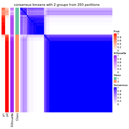
consensus_heatmap(res, k = 3)
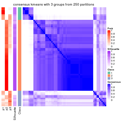
consensus_heatmap(res, k = 4)
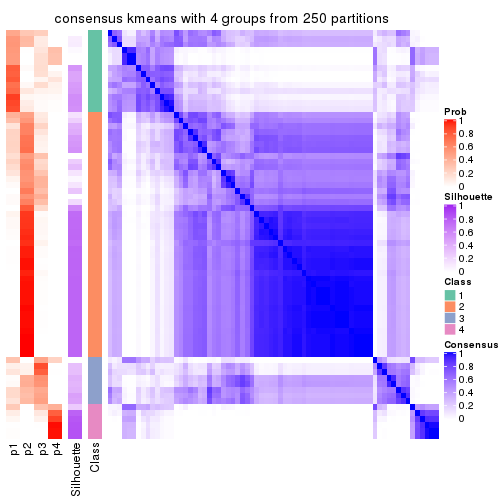
consensus_heatmap(res, k = 5)
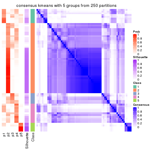
consensus_heatmap(res, k = 6)
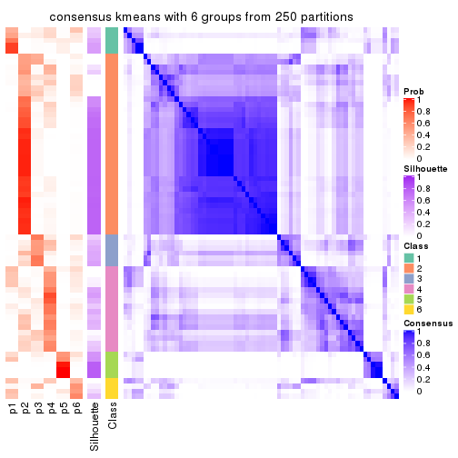
Heatmaps for the membership of samples in all partitions to see how consistent they are:
membership_heatmap(res, k = 2)
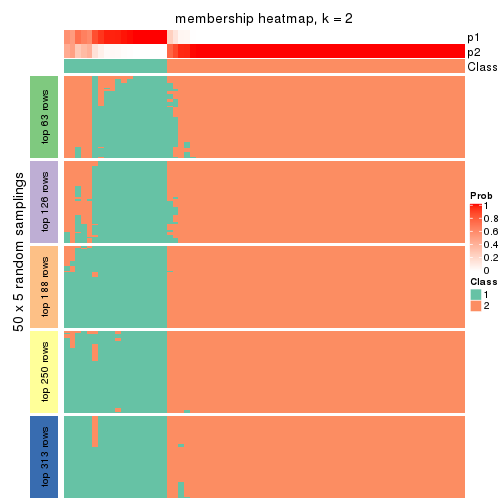
membership_heatmap(res, k = 3)
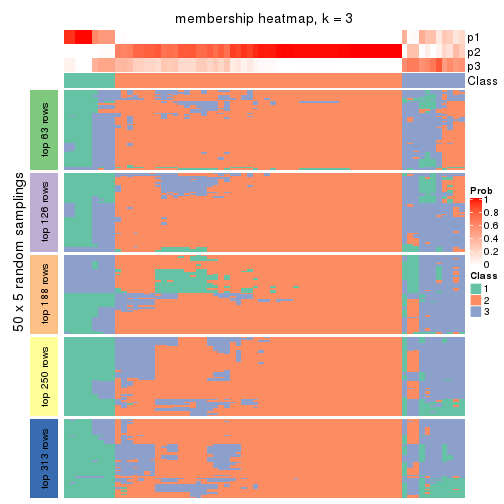
membership_heatmap(res, k = 4)
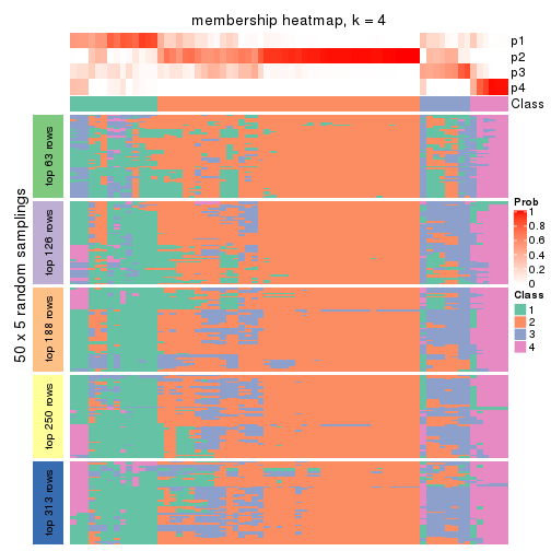
membership_heatmap(res, k = 5)
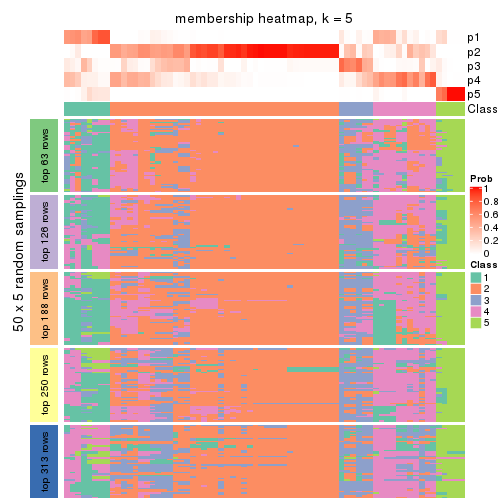
membership_heatmap(res, k = 6)
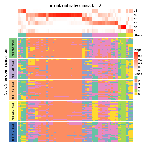
As soon as we have had the classes for columns, we can look for signatures which are significantly different between classes which can be candidate marks for certain classes. Following are the heatmaps for signatures.
Signature heatmaps where rows are scaled:
get_signatures(res, k = 2)
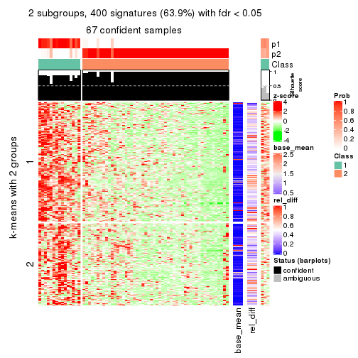
get_signatures(res, k = 3)
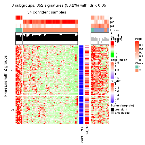
get_signatures(res, k = 4)
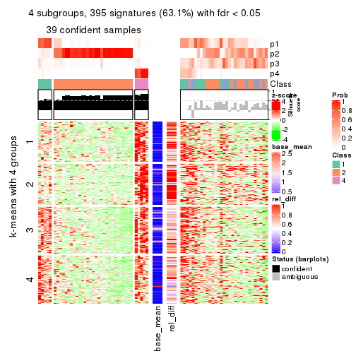
get_signatures(res, k = 5)
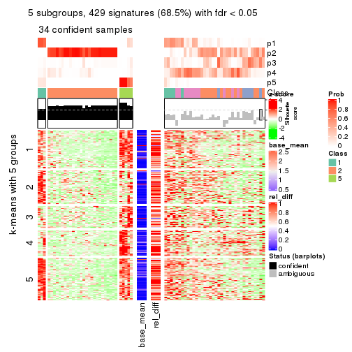
get_signatures(res, k = 6)
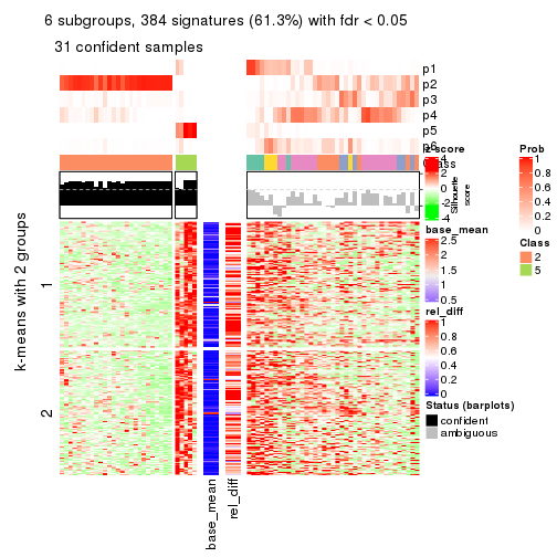
Signature heatmaps where rows are not scaled:
get_signatures(res, k = 2, scale_rows = FALSE)
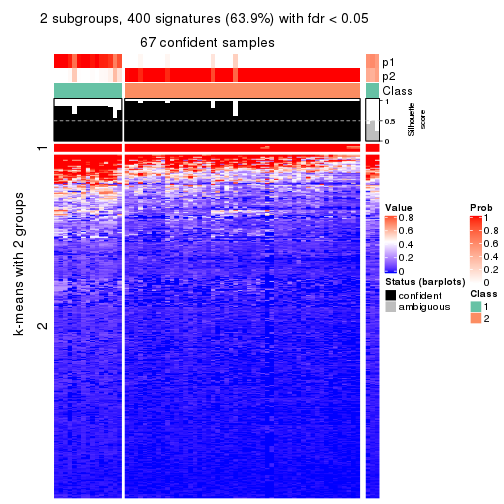
get_signatures(res, k = 3, scale_rows = FALSE)
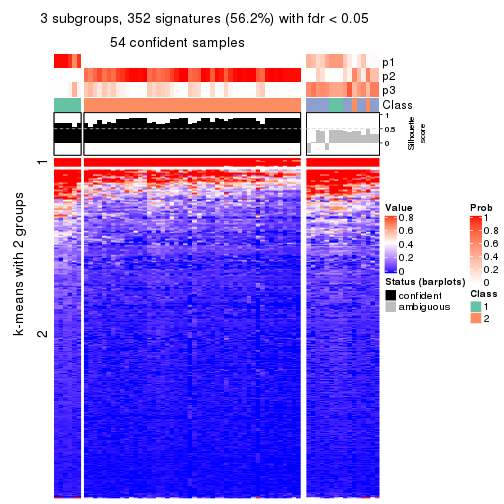
get_signatures(res, k = 4, scale_rows = FALSE)
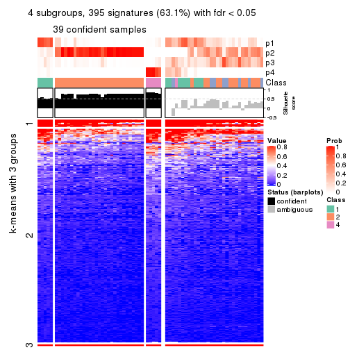
get_signatures(res, k = 5, scale_rows = FALSE)
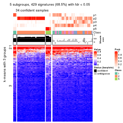
get_signatures(res, k = 6, scale_rows = FALSE)
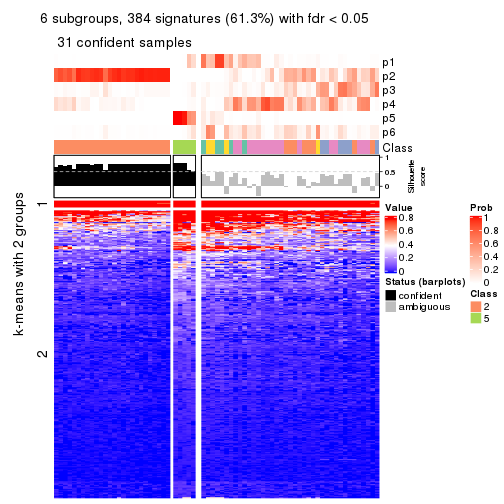
Compare the overlap of signatures from different k:
compare_signatures(res)
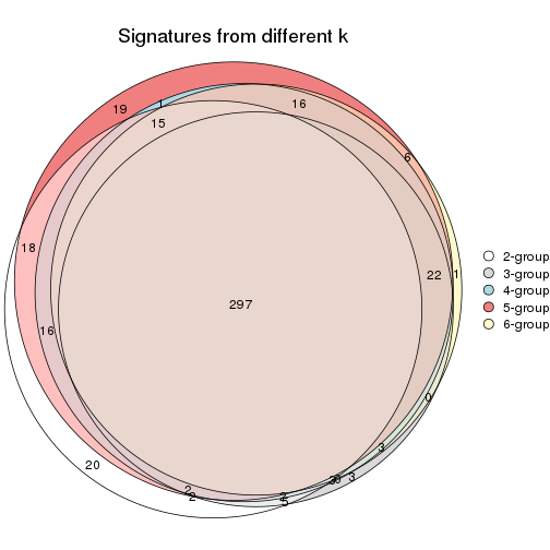
get_signature() returns a data frame invisibly. TO get the list of signatures, the function
call should be assigned to a variable explicitly. In following code, if plot argument is set
to FALSE, no heatmap is plotted while only the differential analysis is performed.
# code only for demonstration
tb = get_signature(res, k = ..., plot = FALSE)
An example of the output of tb is:
#>   which_row         fdr    mean_1    mean_2 scaled_mean_1 scaled_mean_2 km
#> 1        38 0.042760348  8.373488  9.131774    -0.5533452     0.5164555  1
#> 2        40 0.018707592  7.106213  8.469186    -0.6173731     0.5762149  1
#> 3        55 0.019134737 10.221463 11.207825    -0.6159697     0.5749050  1
#> 4        59 0.006059896  5.921854  7.869574    -0.6899429     0.6439467  1
#> 5        60 0.018055526  8.928898 10.211722    -0.6204761     0.5791110  1
#> 6        98 0.009384629 15.714769 14.887706     0.6635654    -0.6193277  2
...
The columns in tb are:
which_row: row indices corresponding to the input matrix.fdr: FDR for the differential test. mean_x: The mean value in group x.scaled_mean_x: The mean value in group x after rows are scaled.km: Row groups if k-means clustering is applied to rows.UMAP plot which shows how samples are separated.
dimension_reduction(res, k = 2, method = "UMAP")
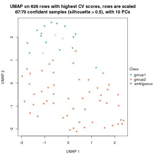
dimension_reduction(res, k = 3, method = "UMAP")
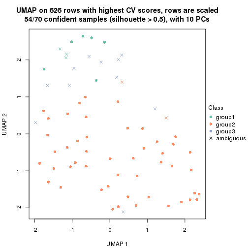
dimension_reduction(res, k = 4, method = "UMAP")
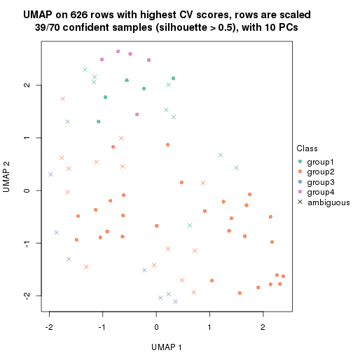
dimension_reduction(res, k = 5, method = "UMAP")
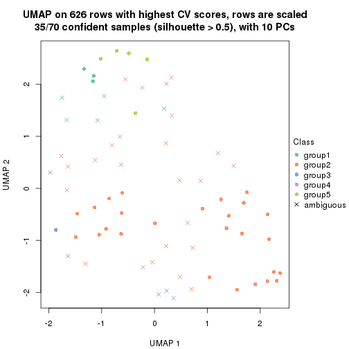
dimension_reduction(res, k = 6, method = "UMAP")
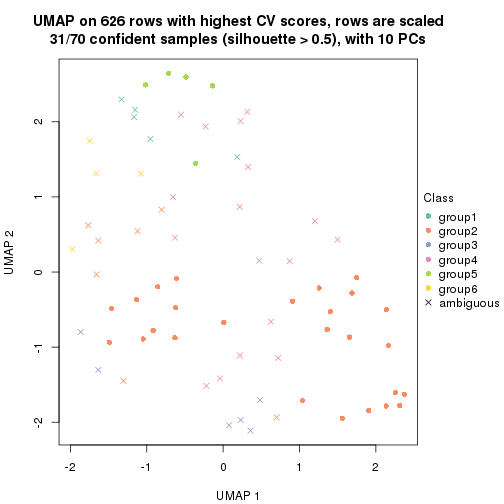
Following heatmap shows how subgroups are split when increasing k:
collect_classes(res)
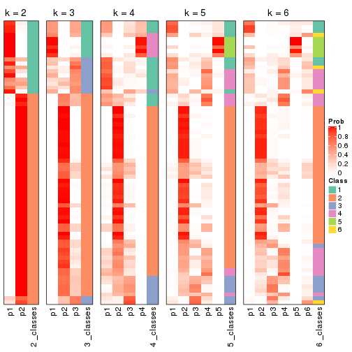
If matrix rows can be associated to genes, consider to use functional_enrichment(res,
...) to perform function enrichment for the signature genes. See this vignette for more detailed explanations.
The object with results only for a single top-value method and a single partition method can be extracted as:
res = res_list["CV", "skmeans"]
# you can also extract it by
# res = res_list["CV:skmeans"]
A summary of res and all the functions that can be applied to it:
res
#> A 'ConsensusPartition' object with k = 2, 3, 4, 5, 6.
#>   On a matrix with 626 rows and 70 columns.
#>   Top rows (63, 126, 188, 250, 313) are extracted by 'CV' method.
#>   Subgroups are detected by 'skmeans' method.
#>   Performed in total 1250 partitions by row resampling.
#>   Best k for subgroups seems to be 2.
#>
#> Following methods can be applied to this 'ConsensusPartition' object:
#>  [1] "cola_report"             "collect_classes"         "collect_plots"
#>  [4] "collect_stats"           "colnames"                "compare_signatures"
#>  [7] "consensus_heatmap"       "dimension_reduction"     "functional_enrichment"
#> [10] "get_anno_col"            "get_anno"                "get_classes"
#> [13] "get_consensus"           "get_matrix"              "get_membership"
#> [16] "get_param"               "get_signatures"          "get_stats"
#> [19] "is_best_k"               "is_stable_k"             "membership_heatmap"
#> [22] "ncol"                    "nrow"                    "plot_ecdf"
#> [25] "rownames"                "select_partition_number" "show"
#> [28] "suggest_best_k"          "test_to_known_factors"
collect_plots() function collects all the plots made from res for all k (number of partitions)
into one single page to provide an easy and fast comparison between different k.
collect_plots(res)
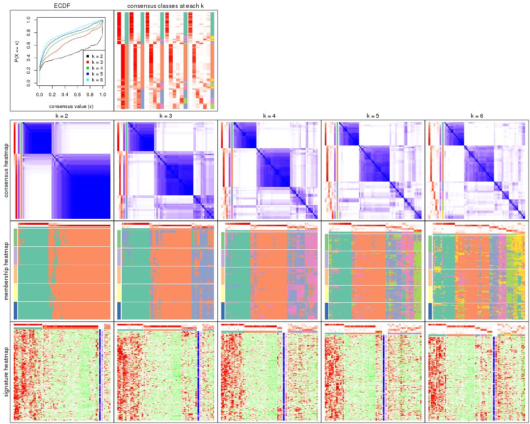
The plots are:
k and the heatmap of
predicted classes for each k.k.k.k.All the plots in panels can be made by individual functions and they are plotted later in this section.
select_partition_number() produces several plots showing different
statistics for choosing “optimized” k. There are following statistics:
k;k, the area increased is defined as \(A_k - A_{k-1}\).The detailed explanations of these statistics can be found in the cola vignette.
Generally speaking, lower PAC score, higher mean silhouette score or higher
concordance corresponds to better partition. Rand index and Jaccard index
measure how similar the current partition is compared to partition with k-1.
If they are too similar, we won't accept k is better than k-1.
select_partition_number(res)
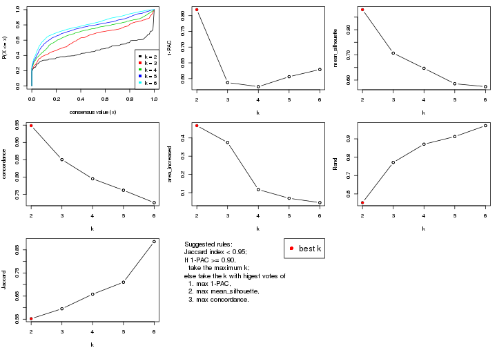
The numeric values for all these statistics can be obtained by get_stats().
get_stats(res)
#>   k 1-PAC mean_silhouette concordance area_increased  Rand Jaccard
#> 2 2 0.819           0.880       0.949         0.4674 0.552   0.552
#> 3 3 0.587           0.707       0.850         0.3752 0.771   0.595
#> 4 4 0.574           0.647       0.795         0.1170 0.871   0.658
#> 5 5 0.606           0.585       0.762         0.0695 0.912   0.710
#> 6 6 0.629           0.574       0.726         0.0452 0.972   0.885
suggest_best_k() suggests the best \(k\) based on these statistics. The rules are as follows:
suggest_best_k(res)
#> [1] 2
Following shows the table of the partitions (You need to click the show/hide
code output link to see it). The membership matrix (columns with name p*)
is inferred by
clue::cl_consensus()
function with the SE method. Basically the value in the membership matrix
represents the probability to belong to a certain group. The finall class
label for an item is determined with the group with highest probability it
belongs to.
In get_classes() function, the entropy is calculated from the membership
matrix and the silhouette score is calculated from the consensus matrix.
cbind(get_classes(res, k = 2), get_membership(res, k = 2))
#>           class entropy silhouette    p1    p2
#> SRR837437     2  0.0000      0.933 0.000 1.000
#> SRR837438     2  0.9522      0.421 0.372 0.628
#> SRR837439     2  0.0000      0.933 0.000 1.000
#> SRR837440     2  0.0000      0.933 0.000 1.000
#> SRR837441     2  0.0000      0.933 0.000 1.000
#> SRR837442     2  0.0000      0.933 0.000 1.000
#> SRR837443     2  0.0000      0.933 0.000 1.000
#> SRR837444     2  0.1184      0.925 0.016 0.984
#> SRR837445     2  0.0000      0.933 0.000 1.000
#> SRR837446     2  0.0000      0.933 0.000 1.000
#> SRR837447     1  0.0000      0.966 1.000 0.000
#> SRR837448     1  0.0000      0.966 1.000 0.000
#> SRR837449     1  0.2423      0.939 0.960 0.040
#> SRR837450     1  0.0000      0.966 1.000 0.000
#> SRR837451     2  0.0000      0.933 0.000 1.000
#> SRR837452     2  0.0000      0.933 0.000 1.000
#> SRR837453     2  0.0000      0.933 0.000 1.000
#> SRR837454     2  0.0000      0.933 0.000 1.000
#> SRR837455     1  0.0000      0.966 1.000 0.000
#> SRR837456     1  0.0000      0.966 1.000 0.000
#> SRR837457     2  0.0000      0.933 0.000 1.000
#> SRR837458     1  0.0000      0.966 1.000 0.000
#> SRR837459     2  0.0000      0.933 0.000 1.000
#> SRR837460     2  0.0000      0.933 0.000 1.000
#> SRR837461     2  0.0000      0.933 0.000 1.000
#> SRR837462     2  0.8555      0.613 0.280 0.720
#> SRR837463     2  0.9983      0.112 0.476 0.524
#> SRR837464     2  0.0000      0.933 0.000 1.000
#> SRR837465     2  0.2948      0.902 0.052 0.948
#> SRR837466     1  0.0000      0.966 1.000 0.000
#> SRR837467     2  0.0000      0.933 0.000 1.000
#> SRR837468     1  0.0938      0.960 0.988 0.012
#> SRR837469     1  0.0000      0.966 1.000 0.000
#> SRR837470     1  0.0000      0.966 1.000 0.000
#> SRR837471     2  0.0000      0.933 0.000 1.000
#> SRR837472     2  0.0000      0.933 0.000 1.000
#> SRR837473     1  0.2948      0.926 0.948 0.052
#> SRR837474     2  0.0000      0.933 0.000 1.000
#> SRR837475     2  0.0000      0.933 0.000 1.000
#> SRR837476     2  0.0000      0.933 0.000 1.000
#> SRR837477     1  0.0000      0.966 1.000 0.000
#> SRR837478     2  0.7139      0.760 0.196 0.804
#> SRR837479     2  0.7674      0.721 0.224 0.776
#> SRR837480     2  0.3431      0.893 0.064 0.936
#> SRR837481     2  0.9358      0.498 0.352 0.648
#> SRR837482     2  0.2043      0.916 0.032 0.968
#> SRR837483     1  0.0000      0.966 1.000 0.000
#> SRR837484     2  0.2236      0.913 0.036 0.964
#> SRR837485     2  0.0376      0.931 0.004 0.996
#> SRR837486     1  0.0000      0.966 1.000 0.000
#> SRR837487     2  0.0000      0.933 0.000 1.000
#> SRR837488     2  0.0000      0.933 0.000 1.000
#> SRR837489     2  0.0000      0.933 0.000 1.000
#> SRR837490     2  0.0000      0.933 0.000 1.000
#> SRR837491     2  0.3733      0.884 0.072 0.928
#> SRR837492     1  0.0000      0.966 1.000 0.000
#> SRR837493     2  0.7219      0.743 0.200 0.800
#> SRR837494     2  0.0000      0.933 0.000 1.000
#> SRR837495     2  0.9909      0.224 0.444 0.556
#> SRR837496     1  0.0000      0.966 1.000 0.000
#> SRR837497     1  0.0000      0.966 1.000 0.000
#> SRR837498     1  0.0672      0.962 0.992 0.008
#> SRR837499     1  0.2236      0.942 0.964 0.036
#> SRR837500     1  0.5737      0.831 0.864 0.136
#> SRR837501     2  0.0672      0.929 0.008 0.992
#> SRR837502     1  0.9686      0.318 0.604 0.396
#> SRR837503     1  0.0376      0.964 0.996 0.004
#> SRR837504     2  0.0000      0.933 0.000 1.000
#> SRR837505     2  0.4298      0.871 0.088 0.912
#> SRR837506     2  0.0000      0.933 0.000 1.000
cbind(get_classes(res, k = 3), get_membership(res, k = 3))
#>           class entropy silhouette    p1    p2    p3
#> SRR837437     2  0.1031     0.8385 0.000 0.976 0.024
#> SRR837438     2  0.9953    -0.1736 0.288 0.368 0.344
#> SRR837439     2  0.0892     0.8388 0.000 0.980 0.020
#> SRR837440     2  0.5138     0.5072 0.000 0.748 0.252
#> SRR837441     2  0.1031     0.8382 0.000 0.976 0.024
#> SRR837442     2  0.0592     0.8383 0.000 0.988 0.012
#> SRR837443     2  0.0747     0.8388 0.000 0.984 0.016
#> SRR837444     2  0.5919     0.5126 0.012 0.712 0.276
#> SRR837445     2  0.4750     0.6127 0.000 0.784 0.216
#> SRR837446     3  0.3038     0.6781 0.000 0.104 0.896
#> SRR837447     1  0.0592     0.9122 0.988 0.000 0.012
#> SRR837448     1  0.0000     0.9140 1.000 0.000 0.000
#> SRR837449     1  0.2926     0.8698 0.924 0.036 0.040
#> SRR837450     1  0.0000     0.9140 1.000 0.000 0.000
#> SRR837451     2  0.1031     0.8393 0.000 0.976 0.024
#> SRR837452     2  0.1411     0.8330 0.000 0.964 0.036
#> SRR837453     2  0.1031     0.8393 0.000 0.976 0.024
#> SRR837454     2  0.1031     0.8393 0.000 0.976 0.024
#> SRR837455     1  0.0237     0.9133 0.996 0.000 0.004
#> SRR837456     1  0.0237     0.9133 0.996 0.000 0.004
#> SRR837457     2  0.1031     0.8393 0.000 0.976 0.024
#> SRR837458     1  0.0000     0.9140 1.000 0.000 0.000
#> SRR837459     2  0.1031     0.8393 0.000 0.976 0.024
#> SRR837460     2  0.1031     0.8393 0.000 0.976 0.024
#> SRR837461     2  0.6308    -0.3099 0.000 0.508 0.492
#> SRR837462     3  0.6984     0.6201 0.040 0.304 0.656
#> SRR837463     3  0.8771     0.5595 0.140 0.304 0.556
#> SRR837464     3  0.5621     0.6248 0.000 0.308 0.692
#> SRR837465     3  0.6919     0.2161 0.016 0.448 0.536
#> SRR837466     1  0.0000     0.9140 1.000 0.000 0.000
#> SRR837467     2  0.1031     0.8391 0.000 0.976 0.024
#> SRR837468     3  0.5058     0.5299 0.244 0.000 0.756
#> SRR837469     1  0.3340     0.8309 0.880 0.000 0.120
#> SRR837470     1  0.0000     0.9140 1.000 0.000 0.000
#> SRR837471     2  0.0237     0.8404 0.000 0.996 0.004
#> SRR837472     2  0.0592     0.8403 0.000 0.988 0.012
#> SRR837473     1  0.2492     0.8802 0.936 0.048 0.016
#> SRR837474     2  0.0592     0.8384 0.000 0.988 0.012
#> SRR837475     2  0.0747     0.8361 0.000 0.984 0.016
#> SRR837476     2  0.0892     0.8394 0.000 0.980 0.020
#> SRR837477     1  0.5327     0.7076 0.728 0.000 0.272
#> SRR837478     3  0.7755     0.1539 0.048 0.460 0.492
#> SRR837479     3  0.3406     0.6790 0.028 0.068 0.904
#> SRR837480     3  0.6769     0.3582 0.016 0.392 0.592
#> SRR837481     3  0.3253     0.6812 0.036 0.052 0.912
#> SRR837482     3  0.1860     0.6900 0.000 0.052 0.948
#> SRR837483     1  0.0000     0.9140 1.000 0.000 0.000
#> SRR837484     3  0.6427     0.6144 0.012 0.348 0.640
#> SRR837485     3  0.5591     0.6509 0.000 0.304 0.696
#> SRR837486     3  0.5529     0.4679 0.296 0.000 0.704
#> SRR837487     2  0.1860     0.8217 0.000 0.948 0.052
#> SRR837488     2  0.1411     0.8330 0.000 0.964 0.036
#> SRR837489     2  0.3038     0.7611 0.000 0.896 0.104
#> SRR837490     2  0.0592     0.8387 0.000 0.988 0.012
#> SRR837491     2  0.5207     0.6958 0.052 0.824 0.124
#> SRR837492     1  0.0000     0.9140 1.000 0.000 0.000
#> SRR837493     2  0.5913     0.6338 0.144 0.788 0.068
#> SRR837494     2  0.1163     0.8399 0.000 0.972 0.028
#> SRR837495     2  0.9757    -0.0879 0.384 0.388 0.228
#> SRR837496     1  0.0592     0.9113 0.988 0.000 0.012
#> SRR837497     1  0.0000     0.9140 1.000 0.000 0.000
#> SRR837498     1  0.3941     0.8259 0.844 0.000 0.156
#> SRR837499     1  0.4921     0.8028 0.816 0.020 0.164
#> SRR837500     1  0.5581     0.7777 0.788 0.036 0.176
#> SRR837501     3  0.5201     0.6857 0.004 0.236 0.760
#> SRR837502     1  0.9034     0.4127 0.556 0.200 0.244
#> SRR837503     1  0.3043     0.8721 0.908 0.008 0.084
#> SRR837504     2  0.4504     0.6276 0.000 0.804 0.196
#> SRR837505     3  0.6159     0.6979 0.048 0.196 0.756
#> SRR837506     3  0.6267     0.4331 0.000 0.452 0.548
cbind(get_classes(res, k = 4), get_membership(res, k = 4))
#>           class entropy silhouette    p1    p2    p3    p4
#> SRR837437     2  0.1488      0.870 0.000 0.956 0.012 0.032
#> SRR837438     4  0.8896      0.234 0.140 0.160 0.196 0.504
#> SRR837439     2  0.1256      0.872 0.000 0.964 0.008 0.028
#> SRR837440     2  0.4525      0.716 0.000 0.804 0.116 0.080
#> SRR837441     2  0.1356      0.871 0.000 0.960 0.008 0.032
#> SRR837442     2  0.1004      0.875 0.000 0.972 0.004 0.024
#> SRR837443     2  0.1151      0.874 0.000 0.968 0.008 0.024
#> SRR837444     4  0.5446      0.456 0.000 0.276 0.044 0.680
#> SRR837445     4  0.4643      0.404 0.000 0.344 0.000 0.656
#> SRR837446     4  0.5392      0.279 0.000 0.040 0.280 0.680
#> SRR837447     1  0.1635      0.877 0.948 0.000 0.008 0.044
#> SRR837448     1  0.0000      0.885 1.000 0.000 0.000 0.000
#> SRR837449     1  0.4371      0.813 0.836 0.020 0.080 0.064
#> SRR837450     1  0.0000      0.885 1.000 0.000 0.000 0.000
#> SRR837451     2  0.0188      0.875 0.000 0.996 0.004 0.000
#> SRR837452     2  0.1706      0.867 0.000 0.948 0.036 0.016
#> SRR837453     2  0.0000      0.874 0.000 1.000 0.000 0.000
#> SRR837454     2  0.0188      0.874 0.000 0.996 0.000 0.004
#> SRR837455     1  0.1722      0.874 0.944 0.000 0.008 0.048
#> SRR837456     1  0.1635      0.876 0.948 0.000 0.008 0.044
#> SRR837457     2  0.0000      0.874 0.000 1.000 0.000 0.000
#> SRR837458     1  0.0000      0.885 1.000 0.000 0.000 0.000
#> SRR837459     2  0.0000      0.874 0.000 1.000 0.000 0.000
#> SRR837460     2  0.0188      0.875 0.000 0.996 0.004 0.000
#> SRR837461     3  0.5808      0.248 0.000 0.424 0.544 0.032
#> SRR837462     3  0.4687      0.523 0.032 0.132 0.808 0.028
#> SRR837463     3  0.6652      0.426 0.064 0.124 0.704 0.108
#> SRR837464     3  0.3907      0.520 0.000 0.140 0.828 0.032
#> SRR837465     3  0.7846      0.161 0.012 0.236 0.500 0.252
#> SRR837466     1  0.0000      0.885 1.000 0.000 0.000 0.000
#> SRR837467     2  0.0336      0.875 0.000 0.992 0.008 0.000
#> SRR837468     3  0.3342      0.489 0.100 0.000 0.868 0.032
#> SRR837469     1  0.3933      0.724 0.792 0.000 0.200 0.008
#> SRR837470     1  0.0000      0.885 1.000 0.000 0.000 0.000
#> SRR837471     2  0.2654      0.828 0.000 0.888 0.004 0.108
#> SRR837472     2  0.1978      0.855 0.000 0.928 0.004 0.068
#> SRR837473     1  0.4322      0.752 0.828 0.060 0.008 0.104
#> SRR837474     2  0.2124      0.854 0.000 0.924 0.008 0.068
#> SRR837475     2  0.2011      0.850 0.000 0.920 0.000 0.080
#> SRR837476     2  0.1743      0.864 0.000 0.940 0.004 0.056
#> SRR837477     4  0.5599      0.408 0.316 0.000 0.040 0.644
#> SRR837478     4  0.5992      0.471 0.016 0.176 0.092 0.716
#> SRR837479     4  0.6174      0.214 0.024 0.032 0.316 0.628
#> SRR837480     4  0.5280      0.458 0.000 0.128 0.120 0.752
#> SRR837481     3  0.5669      0.130 0.004 0.016 0.516 0.464
#> SRR837482     3  0.5345      0.211 0.000 0.012 0.560 0.428
#> SRR837483     1  0.0000      0.885 1.000 0.000 0.000 0.000
#> SRR837484     3  0.6933      0.422 0.000 0.300 0.560 0.140
#> SRR837485     3  0.6977      0.447 0.000 0.204 0.584 0.212
#> SRR837486     3  0.6796      0.337 0.252 0.000 0.596 0.152
#> SRR837487     2  0.2125      0.836 0.000 0.920 0.076 0.004
#> SRR837488     2  0.0921      0.869 0.000 0.972 0.028 0.000
#> SRR837489     2  0.4789      0.696 0.000 0.772 0.056 0.172
#> SRR837490     2  0.2773      0.835 0.000 0.900 0.028 0.072
#> SRR837491     2  0.7346      0.298 0.012 0.544 0.136 0.308
#> SRR837492     1  0.0469      0.882 0.988 0.000 0.000 0.012
#> SRR837493     2  0.8324      0.251 0.064 0.520 0.152 0.264
#> SRR837494     2  0.0469      0.875 0.000 0.988 0.000 0.012
#> SRR837495     4  0.4849      0.515 0.080 0.116 0.008 0.796
#> SRR837496     1  0.0817      0.881 0.976 0.000 0.000 0.024
#> SRR837497     1  0.0524      0.885 0.988 0.000 0.004 0.008
#> SRR837498     1  0.6013      0.651 0.684 0.000 0.196 0.120
#> SRR837499     1  0.5038      0.563 0.652 0.000 0.012 0.336
#> SRR837500     1  0.5376      0.437 0.588 0.000 0.016 0.396
#> SRR837501     3  0.5902      0.531 0.000 0.140 0.700 0.160
#> SRR837502     4  0.7875      0.137 0.380 0.076 0.064 0.480
#> SRR837503     1  0.2799      0.829 0.884 0.000 0.008 0.108
#> SRR837504     2  0.4888      0.577 0.000 0.740 0.224 0.036
#> SRR837505     3  0.5628      0.535 0.000 0.132 0.724 0.144
#> SRR837506     2  0.6949     -0.195 0.000 0.480 0.408 0.112
cbind(get_classes(res, k = 5), get_membership(res, k = 5))
#>           class entropy silhouette    p1    p2    p3    p4    p5
#> SRR837437     2  0.1901     0.8389 0.000 0.928 0.004 0.056 0.012
#> SRR837438     4  0.6170     0.3736 0.044 0.076 0.052 0.704 0.124
#> SRR837439     2  0.1626     0.8387 0.000 0.940 0.000 0.044 0.016
#> SRR837440     2  0.5510     0.6193 0.000 0.696 0.196 0.056 0.052
#> SRR837441     2  0.2437     0.8318 0.000 0.904 0.004 0.060 0.032
#> SRR837442     2  0.1862     0.8437 0.000 0.932 0.004 0.048 0.016
#> SRR837443     2  0.1956     0.8373 0.000 0.928 0.008 0.052 0.012
#> SRR837444     4  0.6433     0.2153 0.000 0.156 0.224 0.592 0.028
#> SRR837445     4  0.6105     0.2332 0.000 0.212 0.196 0.588 0.004
#> SRR837446     3  0.6104     0.4195 0.000 0.032 0.616 0.256 0.096
#> SRR837447     1  0.3372     0.7844 0.852 0.000 0.008 0.088 0.052
#> SRR837448     1  0.0162     0.8298 0.996 0.000 0.004 0.000 0.000
#> SRR837449     1  0.6038     0.6607 0.700 0.012 0.080 0.124 0.084
#> SRR837450     1  0.0162     0.8298 0.996 0.000 0.004 0.000 0.000
#> SRR837451     2  0.1082     0.8440 0.000 0.964 0.000 0.008 0.028
#> SRR837452     2  0.4215     0.7942 0.000 0.816 0.064 0.052 0.068
#> SRR837453     2  0.0854     0.8443 0.000 0.976 0.004 0.008 0.012
#> SRR837454     2  0.0162     0.8415 0.000 0.996 0.000 0.004 0.000
#> SRR837455     1  0.4046     0.7543 0.804 0.000 0.008 0.120 0.068
#> SRR837456     1  0.4046     0.7532 0.804 0.000 0.008 0.120 0.068
#> SRR837457     2  0.0671     0.8434 0.000 0.980 0.004 0.000 0.016
#> SRR837458     1  0.0290     0.8304 0.992 0.000 0.000 0.000 0.008
#> SRR837459     2  0.0404     0.8417 0.000 0.988 0.000 0.000 0.012
#> SRR837460     2  0.0794     0.8445 0.000 0.972 0.000 0.000 0.028
#> SRR837461     5  0.5349     0.4499 0.000 0.300 0.048 0.016 0.636
#> SRR837462     5  0.2227     0.7268 0.004 0.048 0.032 0.000 0.916
#> SRR837463     5  0.3370     0.7008 0.012 0.044 0.012 0.064 0.868
#> SRR837464     5  0.3209     0.7122 0.000 0.060 0.068 0.008 0.864
#> SRR837465     5  0.5694     0.6068 0.004 0.096 0.048 0.144 0.708
#> SRR837466     1  0.0000     0.8300 1.000 0.000 0.000 0.000 0.000
#> SRR837467     2  0.2086     0.8376 0.000 0.924 0.008 0.020 0.048
#> SRR837468     5  0.3995     0.5710 0.060 0.000 0.152 0.000 0.788
#> SRR837469     1  0.5091     0.5243 0.648 0.000 0.016 0.032 0.304
#> SRR837470     1  0.1300     0.8260 0.956 0.000 0.000 0.016 0.028
#> SRR837471     2  0.4015     0.7221 0.000 0.768 0.012 0.204 0.016
#> SRR837472     2  0.3154     0.7890 0.000 0.836 0.004 0.148 0.012
#> SRR837473     1  0.6164     0.4555 0.664 0.052 0.064 0.204 0.016
#> SRR837474     2  0.2920     0.7973 0.000 0.852 0.000 0.132 0.016
#> SRR837475     2  0.3059     0.8000 0.000 0.856 0.008 0.120 0.016
#> SRR837476     2  0.3169     0.7959 0.000 0.840 0.004 0.140 0.016
#> SRR837477     3  0.6771     0.1346 0.232 0.000 0.432 0.332 0.004
#> SRR837478     3  0.6707     0.3378 0.052 0.092 0.560 0.292 0.004
#> SRR837479     3  0.6012     0.4498 0.044 0.032 0.676 0.208 0.040
#> SRR837480     3  0.6122     0.2863 0.004 0.084 0.536 0.364 0.012
#> SRR837481     3  0.4296     0.4748 0.004 0.008 0.792 0.068 0.128
#> SRR837482     3  0.4004     0.4424 0.000 0.004 0.784 0.040 0.172
#> SRR837483     1  0.0290     0.8297 0.992 0.000 0.008 0.000 0.000
#> SRR837484     3  0.6023     0.2638 0.000 0.260 0.572 0.000 0.168
#> SRR837485     3  0.5038     0.3888 0.000 0.164 0.704 0.000 0.132
#> SRR837486     3  0.6132     0.2475 0.224 0.000 0.564 0.000 0.212
#> SRR837487     2  0.3289     0.7960 0.000 0.860 0.088 0.016 0.036
#> SRR837488     2  0.2095     0.8270 0.000 0.920 0.060 0.008 0.012
#> SRR837489     2  0.6152     0.2745 0.000 0.536 0.012 0.348 0.104
#> SRR837490     2  0.3997     0.7123 0.000 0.776 0.004 0.188 0.032
#> SRR837491     4  0.6795     0.2845 0.004 0.304 0.020 0.516 0.156
#> SRR837492     1  0.1074     0.8223 0.968 0.000 0.012 0.016 0.004
#> SRR837493     4  0.7321     0.2293 0.028 0.336 0.020 0.472 0.144
#> SRR837494     2  0.1372     0.8432 0.000 0.956 0.004 0.024 0.016
#> SRR837495     4  0.4266     0.2436 0.012 0.028 0.184 0.772 0.004
#> SRR837496     1  0.0854     0.8296 0.976 0.000 0.008 0.012 0.004
#> SRR837497     1  0.1329     0.8289 0.956 0.000 0.008 0.032 0.004
#> SRR837498     1  0.7077     0.1925 0.428 0.000 0.020 0.216 0.336
#> SRR837499     4  0.5379    -0.1266 0.460 0.000 0.004 0.492 0.044
#> SRR837500     4  0.5633    -0.0315 0.424 0.000 0.008 0.512 0.056
#> SRR837501     3  0.6164     0.0722 0.000 0.116 0.472 0.004 0.408
#> SRR837502     4  0.8439     0.3545 0.280 0.072 0.072 0.448 0.128
#> SRR837503     1  0.3093     0.7272 0.824 0.000 0.000 0.168 0.008
#> SRR837504     2  0.5580     0.5976 0.000 0.692 0.172 0.028 0.108
#> SRR837505     3  0.6387     0.1790 0.004 0.112 0.520 0.012 0.352
#> SRR837506     2  0.6905    -0.0208 0.000 0.456 0.300 0.012 0.232
cbind(get_classes(res, k = 6), get_membership(res, k = 6))
#>           class entropy silhouette    p1    p2    p3    p4    p5    p6
#> SRR837437     2  0.3112     0.7575 0.000 0.856 0.028 0.016 0.008 0.092
#> SRR837438     6  0.6955     0.1652 0.044 0.036 0.056 0.116 0.140 0.608
#> SRR837439     2  0.2728     0.7650 0.000 0.888 0.024 0.016 0.016 0.056
#> SRR837440     2  0.6089     0.5564 0.000 0.628 0.200 0.060 0.028 0.084
#> SRR837441     2  0.3071     0.7574 0.000 0.864 0.024 0.016 0.016 0.080
#> SRR837442     2  0.3108     0.7674 0.000 0.860 0.036 0.024 0.004 0.076
#> SRR837443     2  0.3670     0.7513 0.000 0.836 0.040 0.024 0.028 0.072
#> SRR837444     5  0.6661     0.4634 0.000 0.096 0.068 0.028 0.540 0.268
#> SRR837445     5  0.5785     0.4872 0.000 0.144 0.016 0.016 0.616 0.208
#> SRR837446     5  0.7385     0.3910 0.000 0.040 0.236 0.108 0.488 0.128
#> SRR837447     1  0.3161     0.7210 0.828 0.000 0.000 0.028 0.008 0.136
#> SRR837448     1  0.0458     0.7670 0.984 0.000 0.000 0.000 0.016 0.000
#> SRR837449     1  0.5516     0.5139 0.644 0.004 0.080 0.036 0.004 0.232
#> SRR837450     1  0.0458     0.7670 0.984 0.000 0.000 0.000 0.016 0.000
#> SRR837451     2  0.1946     0.7693 0.000 0.928 0.020 0.024 0.004 0.024
#> SRR837452     2  0.5179     0.6908 0.000 0.728 0.092 0.060 0.020 0.100
#> SRR837453     2  0.2457     0.7668 0.000 0.900 0.036 0.016 0.004 0.044
#> SRR837454     2  0.1059     0.7711 0.000 0.964 0.016 0.004 0.000 0.016
#> SRR837455     1  0.3590     0.6814 0.776 0.000 0.000 0.032 0.004 0.188
#> SRR837456     1  0.3517     0.6824 0.780 0.000 0.000 0.028 0.004 0.188
#> SRR837457     2  0.1294     0.7705 0.000 0.956 0.024 0.008 0.004 0.008
#> SRR837458     1  0.0260     0.7673 0.992 0.000 0.000 0.000 0.000 0.008
#> SRR837459     2  0.1067     0.7695 0.000 0.964 0.024 0.004 0.004 0.004
#> SRR837460     2  0.1226     0.7734 0.000 0.952 0.004 0.040 0.000 0.004
#> SRR837461     4  0.5576     0.4222 0.000 0.284 0.064 0.608 0.012 0.032
#> SRR837462     4  0.3241     0.7194 0.004 0.044 0.096 0.844 0.000 0.012
#> SRR837463     4  0.3802     0.7134 0.016 0.036 0.044 0.832 0.004 0.068
#> SRR837464     4  0.3657     0.7105 0.000 0.036 0.128 0.808 0.000 0.028
#> SRR837465     4  0.4195     0.6272 0.000 0.040 0.016 0.788 0.032 0.124
#> SRR837466     1  0.0363     0.7667 0.988 0.000 0.000 0.000 0.012 0.000
#> SRR837467     2  0.2532     0.7640 0.000 0.884 0.004 0.060 0.000 0.052
#> SRR837468     4  0.4141     0.5750 0.040 0.000 0.204 0.740 0.000 0.016
#> SRR837469     1  0.5078     0.3635 0.592 0.000 0.032 0.344 0.004 0.028
#> SRR837470     1  0.1700     0.7554 0.928 0.000 0.000 0.048 0.000 0.024
#> SRR837471     2  0.6280     0.4987 0.000 0.572 0.036 0.016 0.148 0.228
#> SRR837472     2  0.5537     0.6056 0.000 0.660 0.032 0.012 0.108 0.188
#> SRR837473     1  0.7675     0.0686 0.472 0.036 0.084 0.016 0.148 0.244
#> SRR837474     2  0.5703     0.6135 0.000 0.656 0.044 0.016 0.100 0.184
#> SRR837475     2  0.5714     0.5907 0.000 0.644 0.036 0.016 0.100 0.204
#> SRR837476     2  0.4309     0.7039 0.000 0.760 0.016 0.008 0.060 0.156
#> SRR837477     5  0.3053     0.5988 0.100 0.000 0.036 0.004 0.852 0.008
#> SRR837478     5  0.4037     0.6327 0.024 0.056 0.096 0.004 0.808 0.012
#> SRR837479     5  0.4677     0.5160 0.008 0.008 0.220 0.036 0.712 0.016
#> SRR837480     5  0.3838     0.6475 0.000 0.056 0.096 0.004 0.812 0.032
#> SRR837481     3  0.5083     0.4155 0.000 0.004 0.640 0.068 0.272 0.016
#> SRR837482     3  0.5340     0.4883 0.000 0.008 0.664 0.092 0.208 0.028
#> SRR837483     1  0.0964     0.7659 0.968 0.000 0.016 0.000 0.012 0.004
#> SRR837484     3  0.3425     0.6071 0.000 0.164 0.800 0.028 0.000 0.008
#> SRR837485     3  0.2872     0.6600 0.000 0.088 0.868 0.016 0.024 0.004
#> SRR837486     3  0.5021     0.5189 0.184 0.000 0.704 0.068 0.036 0.008
#> SRR837487     2  0.4052     0.6962 0.000 0.764 0.176 0.008 0.008 0.044
#> SRR837488     2  0.2642     0.7542 0.000 0.864 0.116 0.004 0.004 0.012
#> SRR837489     2  0.6983     0.2514 0.000 0.484 0.044 0.100 0.060 0.312
#> SRR837490     2  0.4489     0.6737 0.000 0.752 0.020 0.060 0.012 0.156
#> SRR837491     6  0.6623     0.2369 0.000 0.240 0.036 0.140 0.036 0.548
#> SRR837492     1  0.2206     0.7285 0.904 0.000 0.008 0.000 0.064 0.024
#> SRR837493     6  0.7166     0.2189 0.020 0.252 0.028 0.160 0.036 0.504
#> SRR837494     2  0.2316     0.7671 0.000 0.908 0.020 0.024 0.004 0.044
#> SRR837495     5  0.4421     0.4229 0.000 0.012 0.004 0.012 0.620 0.352
#> SRR837496     1  0.1492     0.7636 0.940 0.000 0.000 0.000 0.036 0.024
#> SRR837497     1  0.2312     0.7539 0.896 0.000 0.008 0.004 0.012 0.080
#> SRR837498     1  0.6711     0.1534 0.432 0.000 0.028 0.296 0.008 0.236
#> SRR837499     6  0.5829     0.0893 0.408 0.000 0.000 0.016 0.120 0.456
#> SRR837500     6  0.5983     0.1411 0.388 0.000 0.000 0.024 0.124 0.464
#> SRR837501     3  0.6167     0.4879 0.000 0.088 0.616 0.212 0.032 0.052
#> SRR837502     6  0.8953     0.2020 0.244 0.052 0.076 0.084 0.232 0.312
#> SRR837503     1  0.4193     0.6005 0.736 0.000 0.000 0.004 0.072 0.188
#> SRR837504     2  0.5652     0.4105 0.000 0.596 0.284 0.076 0.004 0.040
#> SRR837505     3  0.5396     0.5549 0.000 0.076 0.684 0.184 0.032 0.024
#> SRR837506     2  0.7620    -0.1624 0.000 0.380 0.344 0.148 0.048 0.080
Heatmaps for the consensus matrix. It visualizes the probability of two samples to be in a same group.
consensus_heatmap(res, k = 2)
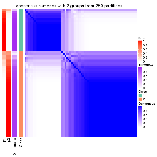
consensus_heatmap(res, k = 3)
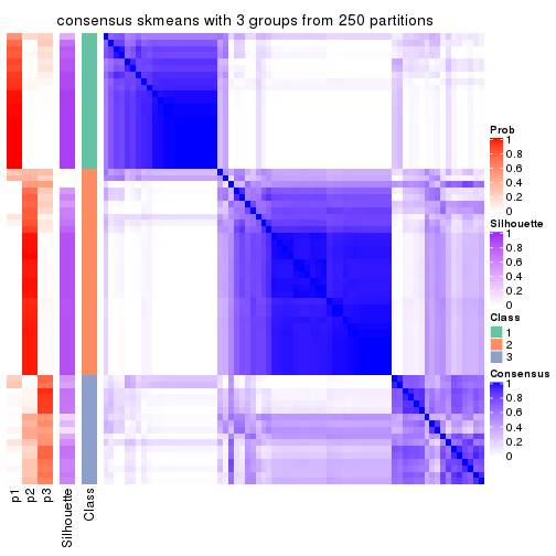
consensus_heatmap(res, k = 4)
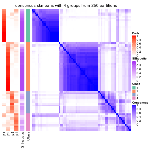
consensus_heatmap(res, k = 5)
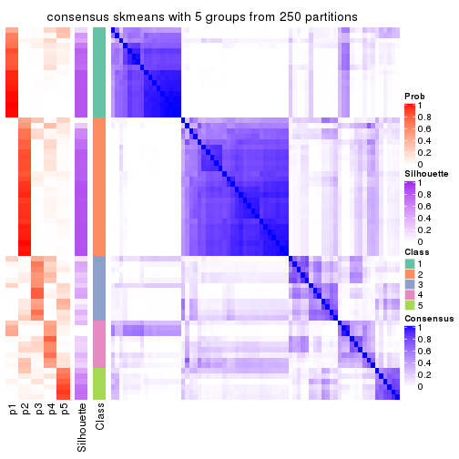
consensus_heatmap(res, k = 6)
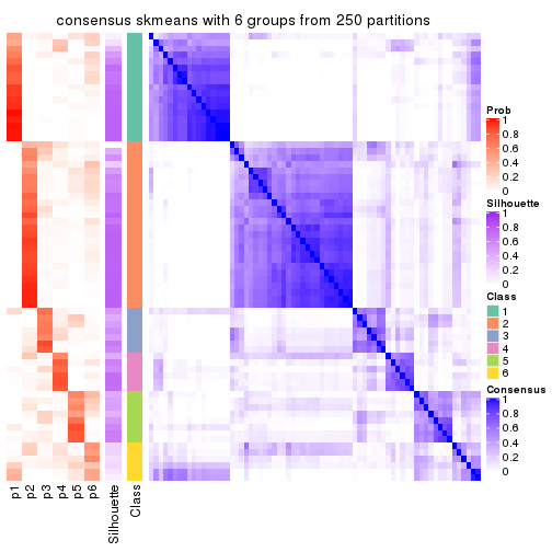
Heatmaps for the membership of samples in all partitions to see how consistent they are:
membership_heatmap(res, k = 2)
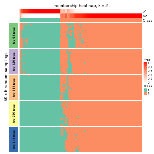
membership_heatmap(res, k = 3)
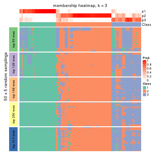
membership_heatmap(res, k = 4)
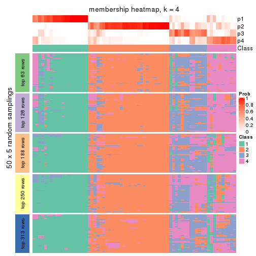
membership_heatmap(res, k = 5)
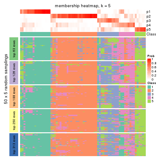
membership_heatmap(res, k = 6)
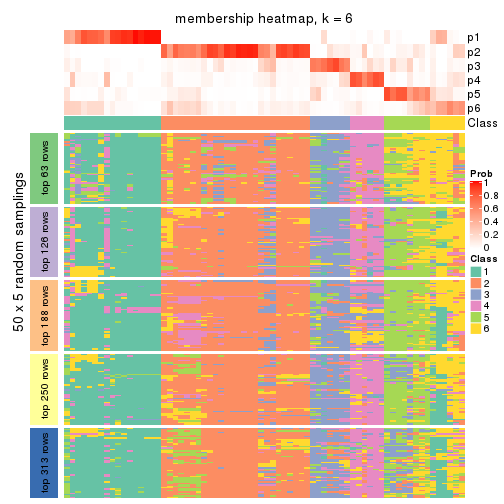
As soon as we have had the classes for columns, we can look for signatures which are significantly different between classes which can be candidate marks for certain classes. Following are the heatmaps for signatures.
Signature heatmaps where rows are scaled:
get_signatures(res, k = 2)
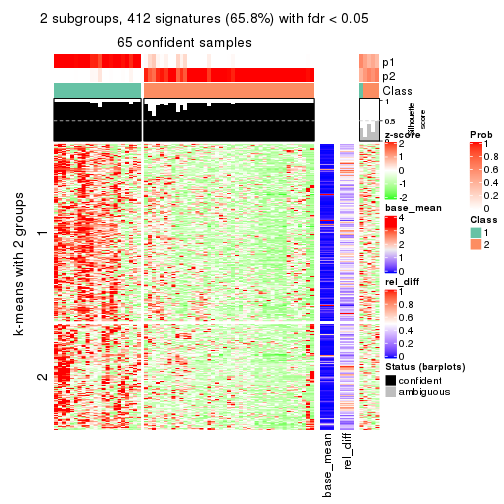
get_signatures(res, k = 3)
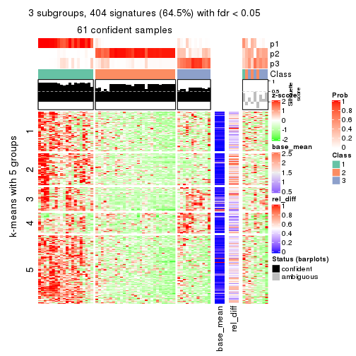
get_signatures(res, k = 4)
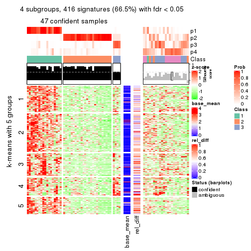
get_signatures(res, k = 5)
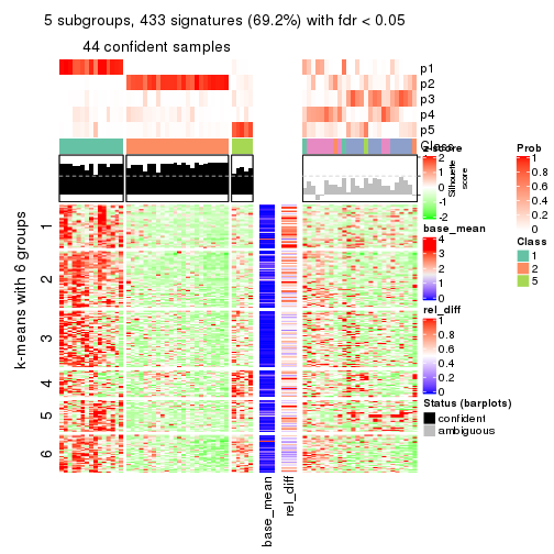
get_signatures(res, k = 6)
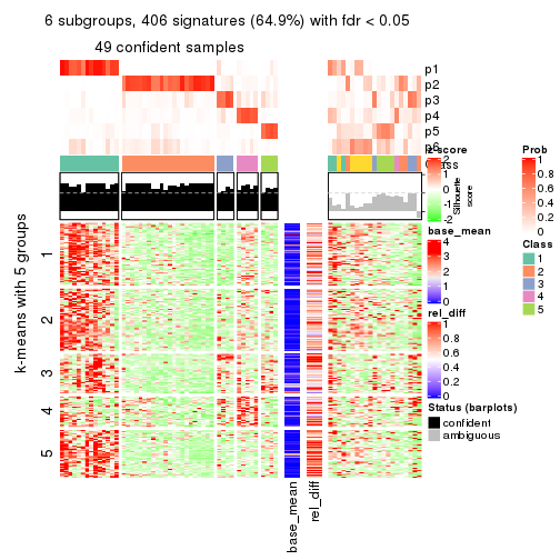
Signature heatmaps where rows are not scaled:
get_signatures(res, k = 2, scale_rows = FALSE)
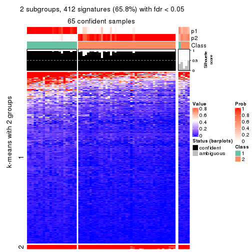
get_signatures(res, k = 3, scale_rows = FALSE)
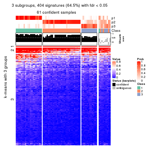
get_signatures(res, k = 4, scale_rows = FALSE)
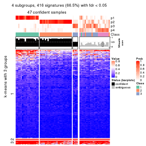
get_signatures(res, k = 5, scale_rows = FALSE)
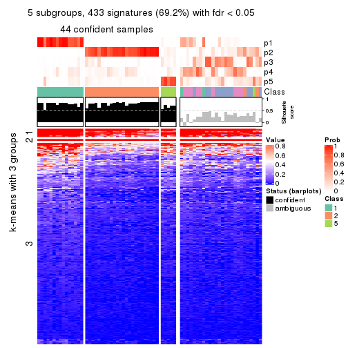
get_signatures(res, k = 6, scale_rows = FALSE)
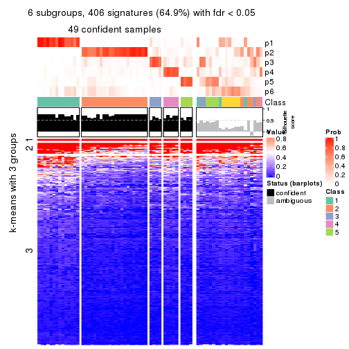
Compare the overlap of signatures from different k:
compare_signatures(res)
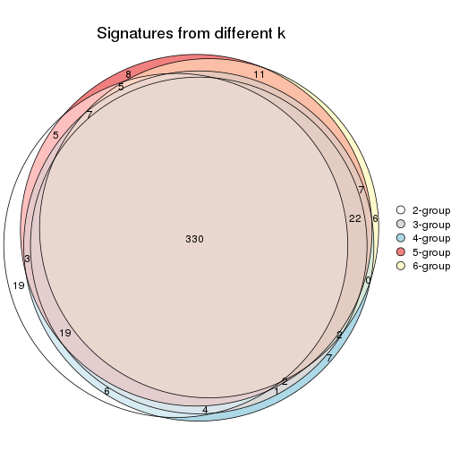
get_signature() returns a data frame invisibly. TO get the list of signatures, the function
call should be assigned to a variable explicitly. In following code, if plot argument is set
to FALSE, no heatmap is plotted while only the differential analysis is performed.
# code only for demonstration
tb = get_signature(res, k = ..., plot = FALSE)
An example of the output of tb is:
#>   which_row         fdr    mean_1    mean_2 scaled_mean_1 scaled_mean_2 km
#> 1        38 0.042760348  8.373488  9.131774    -0.5533452     0.5164555  1
#> 2        40 0.018707592  7.106213  8.469186    -0.6173731     0.5762149  1
#> 3        55 0.019134737 10.221463 11.207825    -0.6159697     0.5749050  1
#> 4        59 0.006059896  5.921854  7.869574    -0.6899429     0.6439467  1
#> 5        60 0.018055526  8.928898 10.211722    -0.6204761     0.5791110  1
#> 6        98 0.009384629 15.714769 14.887706     0.6635654    -0.6193277  2
...
The columns in tb are:
which_row: row indices corresponding to the input matrix.fdr: FDR for the differential test. mean_x: The mean value in group x.scaled_mean_x: The mean value in group x after rows are scaled.km: Row groups if k-means clustering is applied to rows.UMAP plot which shows how samples are separated.
dimension_reduction(res, k = 2, method = "UMAP")
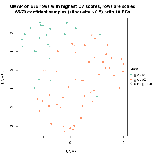
dimension_reduction(res, k = 3, method = "UMAP")
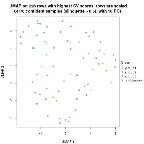
dimension_reduction(res, k = 4, method = "UMAP")
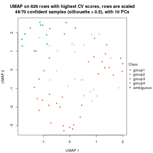
dimension_reduction(res, k = 5, method = "UMAP")
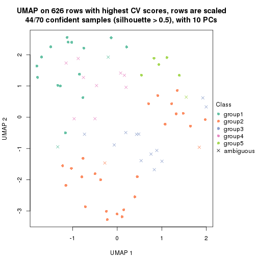
dimension_reduction(res, k = 6, method = "UMAP")
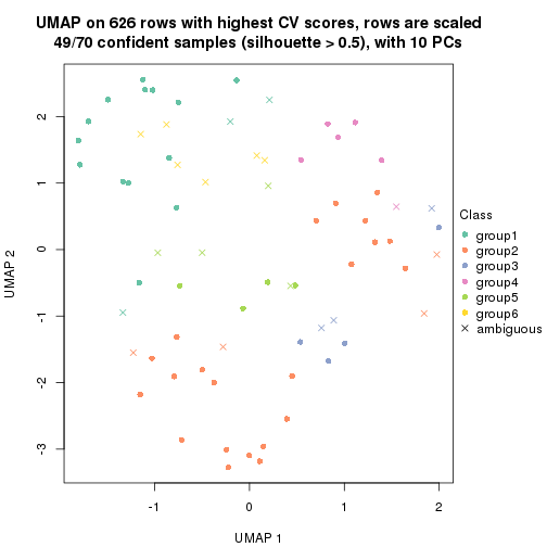
Following heatmap shows how subgroups are split when increasing k:
collect_classes(res)
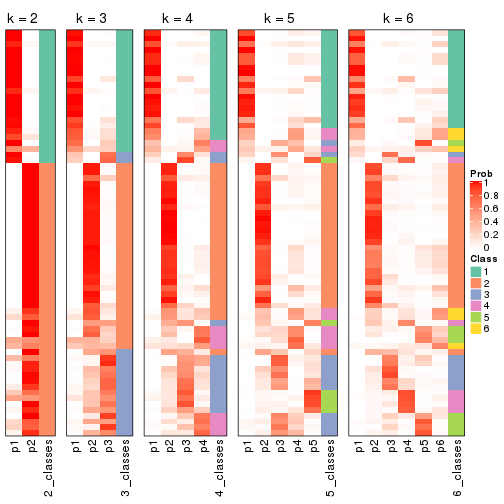
If matrix rows can be associated to genes, consider to use functional_enrichment(res,
...) to perform function enrichment for the signature genes. See this vignette for more detailed explanations.
The object with results only for a single top-value method and a single partition method can be extracted as:
res = res_list["CV", "pam"]
# you can also extract it by
# res = res_list["CV:pam"]
A summary of res and all the functions that can be applied to it:
res
#> A 'ConsensusPartition' object with k = 2, 3, 4, 5, 6.
#>   On a matrix with 626 rows and 70 columns.
#>   Top rows (63, 126, 188, 250, 313) are extracted by 'CV' method.
#>   Subgroups are detected by 'pam' method.
#>   Performed in total 1250 partitions by row resampling.
#>   Best k for subgroups seems to be 2.
#>
#> Following methods can be applied to this 'ConsensusPartition' object:
#>  [1] "cola_report"             "collect_classes"         "collect_plots"
#>  [4] "collect_stats"           "colnames"                "compare_signatures"
#>  [7] "consensus_heatmap"       "dimension_reduction"     "functional_enrichment"
#> [10] "get_anno_col"            "get_anno"                "get_classes"
#> [13] "get_consensus"           "get_matrix"              "get_membership"
#> [16] "get_param"               "get_signatures"          "get_stats"
#> [19] "is_best_k"               "is_stable_k"             "membership_heatmap"
#> [22] "ncol"                    "nrow"                    "plot_ecdf"
#> [25] "rownames"                "select_partition_number" "show"
#> [28] "suggest_best_k"          "test_to_known_factors"
collect_plots() function collects all the plots made from res for all k (number of partitions)
into one single page to provide an easy and fast comparison between different k.
collect_plots(res)
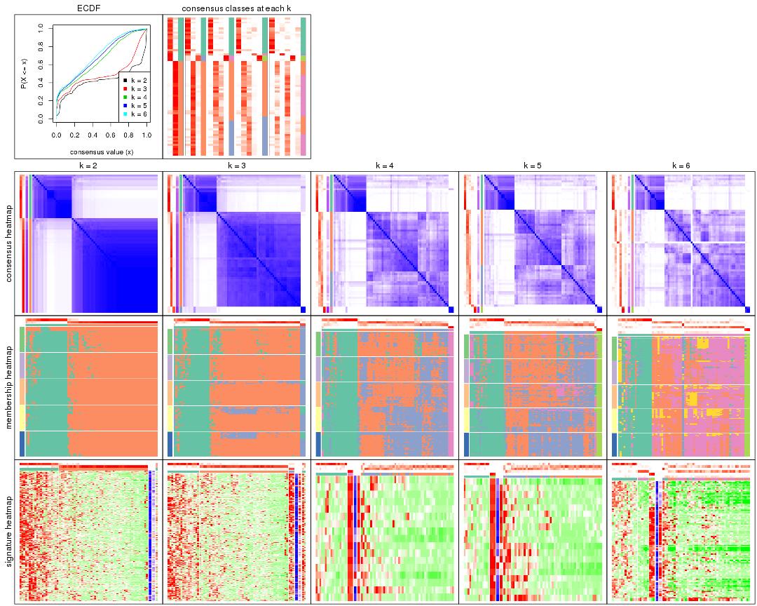
The plots are:
k and the heatmap of
predicted classes for each k.k.k.k.All the plots in panels can be made by individual functions and they are plotted later in this section.
select_partition_number() produces several plots showing different
statistics for choosing “optimized” k. There are following statistics:
k;k, the area increased is defined as \(A_k - A_{k-1}\).The detailed explanations of these statistics can be found in the cola vignette.
Generally speaking, lower PAC score, higher mean silhouette score or higher
concordance corresponds to better partition. Rand index and Jaccard index
measure how similar the current partition is compared to partition with k-1.
If they are too similar, we won't accept k is better than k-1.
select_partition_number(res)
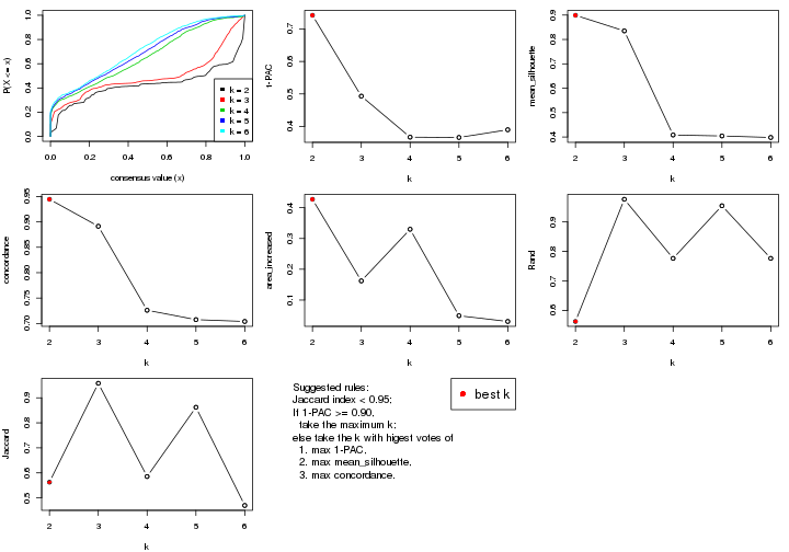
The numeric values for all these statistics can be obtained by get_stats().
get_stats(res)
#>   k 1-PAC mean_silhouette concordance area_increased  Rand Jaccard
#> 2 2 0.742           0.899       0.944         0.4273 0.563   0.563
#> 3 3 0.493           0.835       0.891         0.1622 0.976   0.958
#> 4 4 0.367           0.408       0.726         0.3299 0.776   0.585
#> 5 5 0.366           0.404       0.708         0.0490 0.954   0.862
#> 6 6 0.390           0.398       0.704         0.0304 0.776   0.470
suggest_best_k() suggests the best \(k\) based on these statistics. The rules are as follows:
suggest_best_k(res)
#> [1] 2
Following shows the table of the partitions (You need to click the show/hide
code output link to see it). The membership matrix (columns with name p*)
is inferred by
clue::cl_consensus()
function with the SE method. Basically the value in the membership matrix
represents the probability to belong to a certain group. The finall class
label for an item is determined with the group with highest probability it
belongs to.
In get_classes() function, the entropy is calculated from the membership
matrix and the silhouette score is calculated from the consensus matrix.
cbind(get_classes(res, k = 2), get_membership(res, k = 2))
#>           class entropy silhouette    p1    p2
#> SRR837437     2  0.0000      0.958 0.000 1.000
#> SRR837438     1  0.8713      0.679 0.708 0.292
#> SRR837439     2  0.0000      0.958 0.000 1.000
#> SRR837440     2  0.0000      0.958 0.000 1.000
#> SRR837441     2  0.0000      0.958 0.000 1.000
#> SRR837442     2  0.0000      0.958 0.000 1.000
#> SRR837443     2  0.0000      0.958 0.000 1.000
#> SRR837444     2  0.6973      0.778 0.188 0.812
#> SRR837445     2  0.2423      0.938 0.040 0.960
#> SRR837446     2  0.3274      0.925 0.060 0.940
#> SRR837447     1  0.2236      0.916 0.964 0.036
#> SRR837448     1  0.0000      0.898 1.000 0.000
#> SRR837449     1  0.6623      0.835 0.828 0.172
#> SRR837450     1  0.0672      0.901 0.992 0.008
#> SRR837451     2  0.0000      0.958 0.000 1.000
#> SRR837452     2  0.0376      0.957 0.004 0.996
#> SRR837453     2  0.0000      0.958 0.000 1.000
#> SRR837454     2  0.0000      0.958 0.000 1.000
#> SRR837455     1  0.2236      0.916 0.964 0.036
#> SRR837456     1  0.2236      0.916 0.964 0.036
#> SRR837457     2  0.0000      0.958 0.000 1.000
#> SRR837458     1  0.0000      0.898 1.000 0.000
#> SRR837459     2  0.0000      0.958 0.000 1.000
#> SRR837460     2  0.0000      0.958 0.000 1.000
#> SRR837461     2  0.0000      0.958 0.000 1.000
#> SRR837462     2  0.1633      0.948 0.024 0.976
#> SRR837463     2  0.6623      0.800 0.172 0.828
#> SRR837464     2  0.1184      0.953 0.016 0.984
#> SRR837465     2  0.2778      0.935 0.048 0.952
#> SRR837466     1  0.0000      0.898 1.000 0.000
#> SRR837467     2  0.0000      0.958 0.000 1.000
#> SRR837468     2  0.2948      0.929 0.052 0.948
#> SRR837469     1  0.5059      0.882 0.888 0.112
#> SRR837470     1  0.2043      0.915 0.968 0.032
#> SRR837471     2  0.0000      0.958 0.000 1.000
#> SRR837472     2  0.0000      0.958 0.000 1.000
#> SRR837473     1  0.7376      0.797 0.792 0.208
#> SRR837474     2  0.0000      0.958 0.000 1.000
#> SRR837475     2  0.0938      0.955 0.012 0.988
#> SRR837476     2  0.0000      0.958 0.000 1.000
#> SRR837477     2  0.9044      0.527 0.320 0.680
#> SRR837478     2  0.2778      0.933 0.048 0.952
#> SRR837479     2  0.0376      0.957 0.004 0.996
#> SRR837480     2  0.2423      0.939 0.040 0.960
#> SRR837481     2  0.3274      0.922 0.060 0.940
#> SRR837482     2  0.0376      0.957 0.004 0.996
#> SRR837483     1  0.1633      0.910 0.976 0.024
#> SRR837484     2  0.0376      0.958 0.004 0.996
#> SRR837485     2  0.0672      0.957 0.008 0.992
#> SRR837486     2  0.6438      0.809 0.164 0.836
#> SRR837487     2  0.0000      0.958 0.000 1.000
#> SRR837488     2  0.0000      0.958 0.000 1.000
#> SRR837489     2  0.1633      0.950 0.024 0.976
#> SRR837490     2  0.1184      0.953 0.016 0.984
#> SRR837491     2  0.7219      0.753 0.200 0.800
#> SRR837492     1  0.6623      0.830 0.828 0.172
#> SRR837493     2  0.8386      0.594 0.268 0.732
#> SRR837494     2  0.0000      0.958 0.000 1.000
#> SRR837495     1  0.7815      0.747 0.768 0.232
#> SRR837496     1  0.2236      0.916 0.964 0.036
#> SRR837497     1  0.2423      0.915 0.960 0.040
#> SRR837498     1  0.4298      0.895 0.912 0.088
#> SRR837499     1  0.2236      0.916 0.964 0.036
#> SRR837500     1  0.2236      0.916 0.964 0.036
#> SRR837501     2  0.0376      0.957 0.004 0.996
#> SRR837502     1  0.9963      0.238 0.536 0.464
#> SRR837503     1  0.2236      0.916 0.964 0.036
#> SRR837504     2  0.0000      0.958 0.000 1.000
#> SRR837505     2  0.0938      0.955 0.012 0.988
#> SRR837506     2  0.0000      0.958 0.000 1.000
cbind(get_classes(res, k = 3), get_membership(res, k = 3))
#>           class entropy silhouette    p1    p2    p3
#> SRR837437     2  0.1529      0.913 0.000 0.960 0.040
#> SRR837438     1  0.5728      0.523 0.720 0.272 0.008
#> SRR837439     2  0.2261      0.918 0.000 0.932 0.068
#> SRR837440     2  0.3644      0.915 0.004 0.872 0.124
#> SRR837441     2  0.0747      0.914 0.000 0.984 0.016
#> SRR837442     2  0.1860      0.918 0.000 0.948 0.052
#> SRR837443     2  0.2165      0.918 0.000 0.936 0.064
#> SRR837444     2  0.5728      0.741 0.196 0.772 0.032
#> SRR837445     2  0.2269      0.905 0.040 0.944 0.016
#> SRR837446     2  0.5174      0.887 0.076 0.832 0.092
#> SRR837447     1  0.0592      0.797 0.988 0.012 0.000
#> SRR837448     3  0.3941      1.000 0.156 0.000 0.844
#> SRR837449     1  0.4062      0.679 0.836 0.164 0.000
#> SRR837450     3  0.3941      1.000 0.156 0.000 0.844
#> SRR837451     2  0.3038      0.906 0.000 0.896 0.104
#> SRR837452     2  0.0848      0.912 0.008 0.984 0.008
#> SRR837453     2  0.3267      0.904 0.000 0.884 0.116
#> SRR837454     2  0.3267      0.904 0.000 0.884 0.116
#> SRR837455     1  0.0000      0.794 1.000 0.000 0.000
#> SRR837456     1  0.0424      0.796 0.992 0.008 0.000
#> SRR837457     2  0.3755      0.902 0.008 0.872 0.120
#> SRR837458     1  0.5621      0.338 0.692 0.000 0.308
#> SRR837459     2  0.3755      0.903 0.008 0.872 0.120
#> SRR837460     2  0.3038      0.905 0.000 0.896 0.104
#> SRR837461     2  0.1031      0.912 0.000 0.976 0.024
#> SRR837462     2  0.2982      0.909 0.024 0.920 0.056
#> SRR837463     2  0.5470      0.787 0.168 0.796 0.036
#> SRR837464     2  0.2443      0.912 0.028 0.940 0.032
#> SRR837465     2  0.3028      0.898 0.048 0.920 0.032
#> SRR837466     3  0.3941      1.000 0.156 0.000 0.844
#> SRR837467     2  0.0424      0.912 0.000 0.992 0.008
#> SRR837468     2  0.3375      0.900 0.048 0.908 0.044
#> SRR837469     1  0.3207      0.756 0.904 0.084 0.012
#> SRR837470     1  0.0237      0.793 0.996 0.000 0.004
#> SRR837471     2  0.0892      0.916 0.000 0.980 0.020
#> SRR837472     2  0.2448      0.913 0.000 0.924 0.076
#> SRR837473     1  0.4953      0.666 0.808 0.176 0.016
#> SRR837474     2  0.3192      0.910 0.000 0.888 0.112
#> SRR837475     2  0.3695      0.905 0.012 0.880 0.108
#> SRR837476     2  0.2878      0.908 0.000 0.904 0.096
#> SRR837477     2  0.6800      0.530 0.308 0.660 0.032
#> SRR837478     2  0.4281      0.898 0.072 0.872 0.056
#> SRR837479     2  0.1832      0.908 0.008 0.956 0.036
#> SRR837480     2  0.3369      0.893 0.052 0.908 0.040
#> SRR837481     2  0.3993      0.890 0.064 0.884 0.052
#> SRR837482     2  0.2269      0.908 0.016 0.944 0.040
#> SRR837483     1  0.0592      0.796 0.988 0.012 0.000
#> SRR837484     2  0.3459      0.912 0.012 0.892 0.096
#> SRR837485     2  0.3502      0.917 0.020 0.896 0.084
#> SRR837486     2  0.6402      0.740 0.200 0.744 0.056
#> SRR837487     2  0.3682      0.909 0.008 0.876 0.116
#> SRR837488     2  0.3454      0.905 0.008 0.888 0.104
#> SRR837489     2  0.1711      0.908 0.032 0.960 0.008
#> SRR837490     2  0.1781      0.915 0.020 0.960 0.020
#> SRR837491     2  0.5633      0.726 0.208 0.768 0.024
#> SRR837492     1  0.4228      0.693 0.844 0.148 0.008
#> SRR837493     2  0.6067      0.663 0.236 0.736 0.028
#> SRR837494     2  0.1163      0.917 0.000 0.972 0.028
#> SRR837495     1  0.4796      0.602 0.780 0.220 0.000
#> SRR837496     1  0.0424      0.796 0.992 0.008 0.000
#> SRR837497     1  0.0000      0.794 1.000 0.000 0.000
#> SRR837498     1  0.2400      0.779 0.932 0.064 0.004
#> SRR837499     1  0.0592      0.795 0.988 0.012 0.000
#> SRR837500     1  0.0424      0.796 0.992 0.008 0.000
#> SRR837501     2  0.3845      0.915 0.012 0.872 0.116
#> SRR837502     1  0.7169      0.134 0.520 0.456 0.024
#> SRR837503     1  0.0000      0.794 1.000 0.000 0.000
#> SRR837504     2  0.3965      0.903 0.008 0.860 0.132
#> SRR837505     2  0.3587      0.916 0.020 0.892 0.088
#> SRR837506     2  0.4164      0.905 0.008 0.848 0.144
cbind(get_classes(res, k = 4), get_membership(res, k = 4))
#>           class entropy silhouette    p1    p2    p3    p4
#> SRR837437     3  0.4998  -0.041621 0.000 0.488 0.512 0.000
#> SRR837438     1  0.5772   0.548492 0.672 0.260 0.068 0.000
#> SRR837439     2  0.4661   0.293047 0.000 0.652 0.348 0.000
#> SRR837440     3  0.4985   0.210667 0.000 0.468 0.532 0.000
#> SRR837441     2  0.4877   0.221382 0.000 0.592 0.408 0.000
#> SRR837442     2  0.4605   0.306140 0.000 0.664 0.336 0.000
#> SRR837443     2  0.4888   0.174929 0.000 0.588 0.412 0.000
#> SRR837444     3  0.7012   0.297947 0.156 0.284 0.560 0.000
#> SRR837445     2  0.5691   0.173430 0.028 0.564 0.408 0.000
#> SRR837446     2  0.5929   0.146297 0.048 0.596 0.356 0.000
#> SRR837447     1  0.0376   0.814532 0.992 0.004 0.004 0.000
#> SRR837448     4  0.0000   0.995764 0.000 0.000 0.000 1.000
#> SRR837449     1  0.4633   0.695353 0.780 0.172 0.048 0.000
#> SRR837450     4  0.0000   0.995764 0.000 0.000 0.000 1.000
#> SRR837451     2  0.1637   0.392371 0.000 0.940 0.060 0.000
#> SRR837452     2  0.4585   0.304155 0.000 0.668 0.332 0.000
#> SRR837453     2  0.2469   0.360019 0.000 0.892 0.108 0.000
#> SRR837454     2  0.3074   0.320792 0.000 0.848 0.152 0.000
#> SRR837455     1  0.0000   0.812576 1.000 0.000 0.000 0.000
#> SRR837456     1  0.0000   0.812576 1.000 0.000 0.000 0.000
#> SRR837457     2  0.4830  -0.014155 0.000 0.608 0.392 0.000
#> SRR837458     1  0.6316   0.360604 0.596 0.000 0.080 0.324
#> SRR837459     2  0.3801   0.244120 0.000 0.780 0.220 0.000
#> SRR837460     2  0.1118   0.393609 0.000 0.964 0.036 0.000
#> SRR837461     2  0.4888   0.200843 0.000 0.588 0.412 0.000
#> SRR837462     3  0.3751   0.493598 0.004 0.196 0.800 0.000
#> SRR837463     3  0.6453   0.234359 0.080 0.360 0.560 0.000
#> SRR837464     3  0.5004   0.270758 0.004 0.392 0.604 0.000
#> SRR837465     2  0.5780  -0.000784 0.028 0.496 0.476 0.000
#> SRR837466     4  0.0469   0.991516 0.000 0.000 0.012 0.988
#> SRR837467     2  0.4643   0.286775 0.000 0.656 0.344 0.000
#> SRR837468     3  0.2589   0.490921 0.000 0.116 0.884 0.000
#> SRR837469     1  0.4891   0.630002 0.680 0.012 0.308 0.000
#> SRR837470     1  0.2466   0.773861 0.900 0.000 0.096 0.004
#> SRR837471     2  0.4605   0.321021 0.000 0.664 0.336 0.000
#> SRR837472     2  0.3024   0.410220 0.000 0.852 0.148 0.000
#> SRR837473     1  0.5657   0.611795 0.688 0.068 0.244 0.000
#> SRR837474     2  0.2704   0.395669 0.000 0.876 0.124 0.000
#> SRR837475     2  0.3257   0.301454 0.004 0.844 0.152 0.000
#> SRR837476     2  0.2408   0.409212 0.000 0.896 0.104 0.000
#> SRR837477     3  0.7436   0.289263 0.236 0.252 0.512 0.000
#> SRR837478     3  0.5744   0.253894 0.028 0.436 0.536 0.000
#> SRR837479     3  0.4888   0.178400 0.000 0.412 0.588 0.000
#> SRR837480     3  0.5699   0.251957 0.032 0.380 0.588 0.000
#> SRR837481     3  0.4323   0.502754 0.028 0.184 0.788 0.000
#> SRR837482     3  0.4406   0.428752 0.000 0.300 0.700 0.000
#> SRR837483     1  0.1584   0.807410 0.952 0.000 0.036 0.012
#> SRR837484     3  0.4994   0.195504 0.000 0.480 0.520 0.000
#> SRR837485     3  0.4454   0.375655 0.000 0.308 0.692 0.000
#> SRR837486     3  0.3557   0.451329 0.108 0.036 0.856 0.000
#> SRR837487     2  0.4830  -0.018732 0.000 0.608 0.392 0.000
#> SRR837488     2  0.3172   0.346959 0.000 0.840 0.160 0.000
#> SRR837489     2  0.5339   0.250394 0.020 0.624 0.356 0.000
#> SRR837490     2  0.4632   0.339274 0.004 0.688 0.308 0.000
#> SRR837491     2  0.7092   0.108221 0.148 0.532 0.320 0.000
#> SRR837492     1  0.4155   0.737210 0.828 0.100 0.072 0.000
#> SRR837493     2  0.7250   0.093178 0.220 0.544 0.236 0.000
#> SRR837494     2  0.4103   0.368012 0.000 0.744 0.256 0.000
#> SRR837495     1  0.4589   0.651589 0.784 0.048 0.168 0.000
#> SRR837496     1  0.0188   0.813680 0.996 0.000 0.004 0.000
#> SRR837497     1  0.0707   0.813034 0.980 0.000 0.020 0.000
#> SRR837498     1  0.1854   0.802215 0.940 0.048 0.012 0.000
#> SRR837499     1  0.0188   0.813680 0.996 0.000 0.004 0.000
#> SRR837500     1  0.0188   0.813680 0.996 0.000 0.004 0.000
#> SRR837501     3  0.4661   0.292537 0.000 0.348 0.652 0.000
#> SRR837502     1  0.7657   0.044692 0.464 0.256 0.280 0.000
#> SRR837503     1  0.0188   0.813680 0.996 0.000 0.004 0.000
#> SRR837504     2  0.4999  -0.148490 0.000 0.508 0.492 0.000
#> SRR837505     3  0.4304   0.398828 0.000 0.284 0.716 0.000
#> SRR837506     2  0.4996  -0.137006 0.000 0.516 0.484 0.000
cbind(get_classes(res, k = 5), get_membership(res, k = 5))
#>           class entropy silhouette    p1    p2    p3    p4    p5
#> SRR837437     3  0.4781    -0.2033 0.000 0.428 0.552 0.020 0.000
#> SRR837438     1  0.5532     0.4343 0.644 0.256 0.092 0.008 0.000
#> SRR837439     2  0.4610     0.3890 0.000 0.596 0.388 0.016 0.000
#> SRR837440     3  0.4630     0.2455 0.000 0.396 0.588 0.016 0.000
#> SRR837441     2  0.4723     0.3516 0.000 0.536 0.448 0.016 0.000
#> SRR837442     2  0.4551     0.4234 0.000 0.616 0.368 0.016 0.000
#> SRR837443     2  0.4723     0.2689 0.000 0.536 0.448 0.016 0.000
#> SRR837444     3  0.6389     0.2145 0.160 0.224 0.592 0.024 0.000
#> SRR837445     2  0.5552     0.3196 0.028 0.516 0.432 0.024 0.000
#> SRR837446     2  0.6283     0.2493 0.048 0.548 0.344 0.060 0.000
#> SRR837447     1  0.0162     0.7480 0.996 0.004 0.000 0.000 0.000
#> SRR837448     5  0.0000     0.9654 0.000 0.000 0.000 0.000 1.000
#> SRR837449     1  0.4345     0.5933 0.764 0.172 0.060 0.004 0.000
#> SRR837450     5  0.0162     0.9646 0.000 0.000 0.000 0.004 0.996
#> SRR837451     2  0.1697     0.4125 0.000 0.932 0.060 0.008 0.000
#> SRR837452     2  0.4592     0.4263 0.000 0.644 0.332 0.024 0.000
#> SRR837453     2  0.2304     0.3752 0.000 0.892 0.100 0.008 0.000
#> SRR837454     2  0.2605     0.3208 0.000 0.852 0.148 0.000 0.000
#> SRR837455     1  0.0963     0.7398 0.964 0.000 0.000 0.036 0.000
#> SRR837456     1  0.0963     0.7398 0.964 0.000 0.000 0.036 0.000
#> SRR837457     2  0.4210    -0.1562 0.000 0.588 0.412 0.000 0.000
#> SRR837458     4  0.4216     0.0000 0.120 0.000 0.000 0.780 0.100
#> SRR837459     2  0.3424     0.1853 0.000 0.760 0.240 0.000 0.000
#> SRR837460     2  0.1485     0.4136 0.000 0.948 0.032 0.020 0.000
#> SRR837461     2  0.5369     0.3469 0.000 0.552 0.388 0.060 0.000
#> SRR837462     3  0.3936     0.4614 0.004 0.144 0.800 0.052 0.000
#> SRR837463     3  0.6502     0.0672 0.076 0.328 0.544 0.052 0.000
#> SRR837464     3  0.5291     0.1645 0.004 0.348 0.596 0.052 0.000
#> SRR837465     2  0.5997     0.2122 0.024 0.468 0.452 0.056 0.000
#> SRR837466     5  0.1270     0.9350 0.000 0.000 0.000 0.052 0.948
#> SRR837467     2  0.4608     0.4190 0.000 0.640 0.336 0.024 0.000
#> SRR837468     3  0.3857     0.4728 0.000 0.084 0.808 0.108 0.000
#> SRR837469     1  0.6096     0.2626 0.560 0.008 0.120 0.312 0.000
#> SRR837470     1  0.4620     0.3772 0.652 0.000 0.028 0.320 0.000
#> SRR837471     2  0.4687     0.4375 0.000 0.636 0.336 0.028 0.000
#> SRR837472     2  0.3123     0.4831 0.000 0.828 0.160 0.012 0.000
#> SRR837473     1  0.4969     0.5001 0.676 0.056 0.264 0.004 0.000
#> SRR837474     2  0.2798     0.4262 0.000 0.852 0.140 0.008 0.000
#> SRR837475     2  0.3123     0.2850 0.004 0.812 0.184 0.000 0.000
#> SRR837476     2  0.2612     0.4521 0.000 0.868 0.124 0.008 0.000
#> SRR837477     3  0.7632     0.2499 0.208 0.208 0.488 0.096 0.000
#> SRR837478     3  0.6397     0.2542 0.028 0.348 0.528 0.096 0.000
#> SRR837479     3  0.5815     0.0587 0.000 0.356 0.540 0.104 0.000
#> SRR837480     3  0.6505     0.1020 0.020 0.344 0.512 0.124 0.000
#> SRR837481     3  0.4480     0.4699 0.020 0.116 0.784 0.080 0.000
#> SRR837482     3  0.5102     0.3972 0.000 0.216 0.684 0.100 0.000
#> SRR837483     1  0.3219     0.6956 0.872 0.000 0.032 0.060 0.036
#> SRR837484     3  0.4930     0.3160 0.000 0.388 0.580 0.032 0.000
#> SRR837485     3  0.3977     0.4434 0.000 0.204 0.764 0.032 0.000
#> SRR837486     3  0.3429     0.4739 0.040 0.012 0.848 0.100 0.000
#> SRR837487     2  0.4517    -0.1123 0.000 0.556 0.436 0.008 0.000
#> SRR837488     2  0.3171     0.3430 0.000 0.816 0.176 0.008 0.000
#> SRR837489     2  0.5555     0.3803 0.028 0.580 0.360 0.032 0.000
#> SRR837490     2  0.4853     0.4525 0.008 0.652 0.312 0.028 0.000
#> SRR837491     2  0.6852     0.2868 0.128 0.504 0.328 0.040 0.000
#> SRR837492     1  0.4996     0.6039 0.764 0.092 0.072 0.072 0.000
#> SRR837493     2  0.6798     0.2269 0.204 0.516 0.260 0.020 0.000
#> SRR837494     2  0.4063     0.4721 0.000 0.708 0.280 0.012 0.000
#> SRR837495     1  0.4087     0.5482 0.784 0.040 0.168 0.008 0.000
#> SRR837496     1  0.0000     0.7472 1.000 0.000 0.000 0.000 0.000
#> SRR837497     1  0.0703     0.7456 0.976 0.000 0.024 0.000 0.000
#> SRR837498     1  0.1408     0.7377 0.948 0.044 0.008 0.000 0.000
#> SRR837499     1  0.0000     0.7472 1.000 0.000 0.000 0.000 0.000
#> SRR837500     1  0.0000     0.7472 1.000 0.000 0.000 0.000 0.000
#> SRR837501     3  0.4428     0.3939 0.000 0.268 0.700 0.032 0.000
#> SRR837502     1  0.7091     0.1135 0.464 0.232 0.280 0.024 0.000
#> SRR837503     1  0.0000     0.7472 1.000 0.000 0.000 0.000 0.000
#> SRR837504     3  0.4410     0.2568 0.000 0.440 0.556 0.004 0.000
#> SRR837505     3  0.4114     0.4365 0.000 0.244 0.732 0.024 0.000
#> SRR837506     3  0.4815     0.2382 0.000 0.456 0.524 0.020 0.000
cbind(get_classes(res, k = 6), get_membership(res, k = 6))
#>           class entropy silhouette    p1    p2    p3    p4    p5    p6
#> SRR837437     4  0.4062     0.4468 0.000 0.176 0.000 0.744 0.000 0.080
#> SRR837438     1  0.4539     0.4819 0.644 0.048 0.000 0.304 0.000 0.004
#> SRR837439     4  0.4187     0.4323 0.000 0.168 0.000 0.736 0.000 0.096
#> SRR837440     2  0.5285     0.1587 0.000 0.480 0.000 0.420 0.000 0.100
#> SRR837441     4  0.2608     0.5095 0.000 0.048 0.000 0.872 0.000 0.080
#> SRR837442     4  0.3458     0.4938 0.000 0.112 0.000 0.808 0.000 0.080
#> SRR837443     4  0.4707     0.3302 0.000 0.252 0.000 0.656 0.000 0.092
#> SRR837444     4  0.6673     0.2362 0.160 0.192 0.000 0.532 0.000 0.116
#> SRR837445     4  0.3329     0.5176 0.032 0.052 0.000 0.844 0.000 0.072
#> SRR837446     4  0.6151     0.3403 0.036 0.200 0.000 0.548 0.000 0.216
#> SRR837447     1  0.0291     0.7377 0.992 0.000 0.000 0.004 0.000 0.004
#> SRR837448     5  0.0146     0.9551 0.000 0.000 0.004 0.000 0.996 0.000
#> SRR837449     1  0.3992     0.6155 0.756 0.052 0.000 0.184 0.000 0.008
#> SRR837450     5  0.0000     0.9541 0.000 0.000 0.000 0.000 1.000 0.000
#> SRR837451     4  0.4089    -0.0993 0.000 0.468 0.000 0.524 0.000 0.008
#> SRR837452     4  0.2651     0.5041 0.000 0.112 0.000 0.860 0.000 0.028
#> SRR837453     2  0.4177     0.1100 0.000 0.520 0.000 0.468 0.000 0.012
#> SRR837454     2  0.3804     0.2209 0.000 0.576 0.000 0.424 0.000 0.000
#> SRR837455     1  0.1866     0.7180 0.908 0.000 0.084 0.000 0.000 0.008
#> SRR837456     1  0.1866     0.7180 0.908 0.000 0.084 0.000 0.000 0.008
#> SRR837457     2  0.2730     0.4475 0.000 0.808 0.000 0.192 0.000 0.000
#> SRR837458     3  0.0717     0.0000 0.008 0.000 0.976 0.000 0.016 0.000
#> SRR837459     2  0.3833     0.3140 0.000 0.648 0.000 0.344 0.000 0.008
#> SRR837460     4  0.5226    -0.0727 0.000 0.444 0.000 0.464 0.000 0.092
#> SRR837461     4  0.3268     0.4960 0.000 0.044 0.000 0.812 0.000 0.144
#> SRR837462     4  0.5907    -0.0533 0.004 0.396 0.000 0.424 0.000 0.176
#> SRR837463     4  0.5593     0.3894 0.056 0.144 0.000 0.652 0.000 0.148
#> SRR837464     4  0.5330     0.3146 0.004 0.208 0.000 0.612 0.000 0.176
#> SRR837465     4  0.4002     0.4779 0.012 0.076 0.000 0.776 0.000 0.136
#> SRR837466     5  0.1700     0.9093 0.000 0.000 0.080 0.000 0.916 0.004
#> SRR837467     4  0.2509     0.5068 0.000 0.088 0.000 0.876 0.000 0.036
#> SRR837468     2  0.6005     0.0268 0.000 0.388 0.000 0.376 0.000 0.236
#> SRR837469     1  0.6381     0.0647 0.416 0.020 0.220 0.000 0.000 0.344
#> SRR837470     1  0.5830     0.2799 0.520 0.004 0.224 0.000 0.000 0.252
#> SRR837471     4  0.3054     0.4960 0.000 0.136 0.000 0.828 0.000 0.036
#> SRR837472     4  0.3445     0.3202 0.000 0.260 0.000 0.732 0.000 0.008
#> SRR837473     1  0.4855     0.5409 0.672 0.236 0.000 0.076 0.000 0.016
#> SRR837474     4  0.4707     0.0569 0.000 0.360 0.000 0.584 0.000 0.056
#> SRR837475     2  0.3966     0.2102 0.004 0.552 0.000 0.444 0.000 0.000
#> SRR837476     4  0.4301     0.0655 0.000 0.392 0.000 0.584 0.000 0.024
#> SRR837477     4  0.6910     0.2149 0.192 0.136 0.004 0.516 0.000 0.152
#> SRR837478     4  0.6479     0.1508 0.032 0.292 0.004 0.480 0.000 0.192
#> SRR837479     4  0.5067     0.3948 0.000 0.136 0.004 0.644 0.000 0.216
#> SRR837480     4  0.5438     0.3649 0.020 0.168 0.004 0.648 0.000 0.160
#> SRR837481     4  0.6216    -0.0746 0.016 0.396 0.000 0.400 0.000 0.188
#> SRR837482     4  0.5542     0.1011 0.000 0.384 0.004 0.492 0.000 0.120
#> SRR837483     1  0.5087     0.5859 0.724 0.032 0.056 0.000 0.036 0.152
#> SRR837484     2  0.3855     0.3410 0.000 0.704 0.000 0.272 0.000 0.024
#> SRR837485     2  0.4682     0.3263 0.000 0.680 0.004 0.224 0.000 0.092
#> SRR837486     2  0.6374     0.1545 0.028 0.504 0.004 0.260 0.000 0.204
#> SRR837487     2  0.3695     0.3119 0.000 0.624 0.000 0.376 0.000 0.000
#> SRR837488     2  0.4333     0.1085 0.000 0.512 0.000 0.468 0.000 0.020
#> SRR837489     4  0.3044     0.5195 0.028 0.076 0.000 0.860 0.000 0.036
#> SRR837490     4  0.3314     0.4926 0.008 0.144 0.000 0.816 0.000 0.032
#> SRR837491     4  0.3483     0.5018 0.100 0.028 0.000 0.828 0.000 0.044
#> SRR837492     1  0.4842     0.5924 0.716 0.020 0.004 0.148 0.000 0.112
#> SRR837493     4  0.4714     0.3723 0.188 0.052 0.000 0.716 0.000 0.044
#> SRR837494     4  0.2887     0.4871 0.000 0.120 0.000 0.844 0.000 0.036
#> SRR837495     1  0.3409     0.5846 0.780 0.000 0.000 0.192 0.000 0.028
#> SRR837496     1  0.0000     0.7363 1.000 0.000 0.000 0.000 0.000 0.000
#> SRR837497     1  0.1777     0.7241 0.928 0.024 0.004 0.000 0.000 0.044
#> SRR837498     1  0.1410     0.7329 0.944 0.008 0.000 0.044 0.000 0.004
#> SRR837499     1  0.0000     0.7363 1.000 0.000 0.000 0.000 0.000 0.000
#> SRR837500     1  0.0000     0.7363 1.000 0.000 0.000 0.000 0.000 0.000
#> SRR837501     2  0.5357     0.3741 0.000 0.588 0.000 0.180 0.000 0.232
#> SRR837502     1  0.6275     0.1089 0.440 0.176 0.000 0.360 0.000 0.024
#> SRR837503     1  0.0000     0.7363 1.000 0.000 0.000 0.000 0.000 0.000
#> SRR837504     2  0.3385     0.4682 0.000 0.788 0.000 0.180 0.000 0.032
#> SRR837505     2  0.4527     0.3405 0.000 0.660 0.000 0.272 0.000 0.068
#> SRR837506     2  0.3493     0.4689 0.000 0.800 0.000 0.136 0.000 0.064
Heatmaps for the consensus matrix. It visualizes the probability of two samples to be in a same group.
consensus_heatmap(res, k = 2)
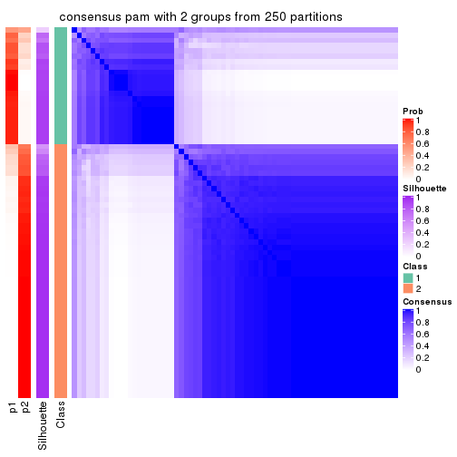
consensus_heatmap(res, k = 3)
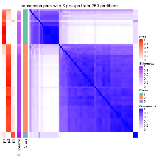
consensus_heatmap(res, k = 4)
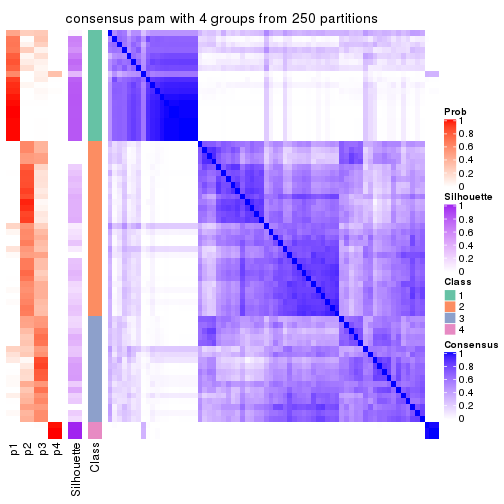
consensus_heatmap(res, k = 5)
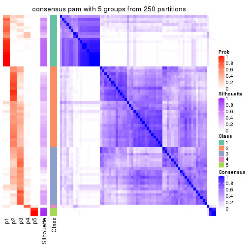
consensus_heatmap(res, k = 6)
Heatmaps for the membership of samples in all partitions to see how consistent they are:
membership_heatmap(res, k = 2)
membership_heatmap(res, k = 3)
membership_heatmap(res, k = 4)
membership_heatmap(res, k = 5)
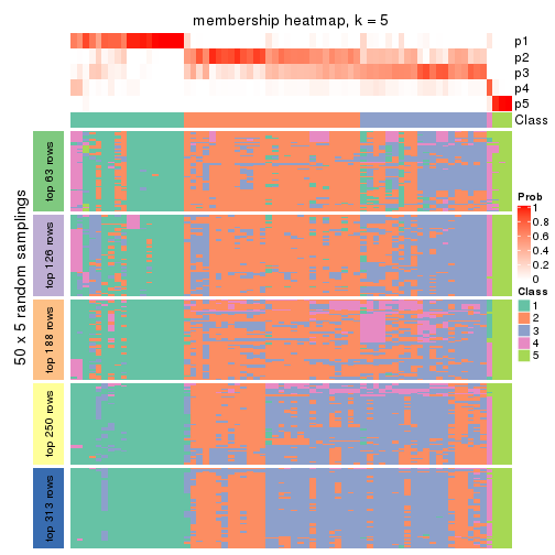
membership_heatmap(res, k = 6)
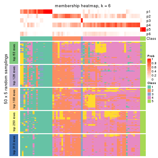
As soon as we have had the classes for columns, we can look for signatures which are significantly different between classes which can be candidate marks for certain classes. Following are the heatmaps for signatures.
Signature heatmaps where rows are scaled:
get_signatures(res, k = 2)
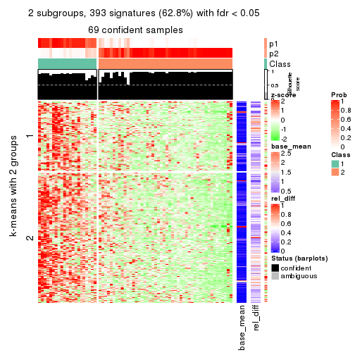
get_signatures(res, k = 3)
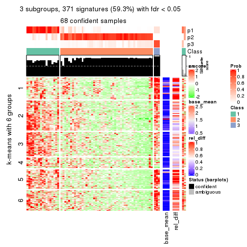
get_signatures(res, k = 4)
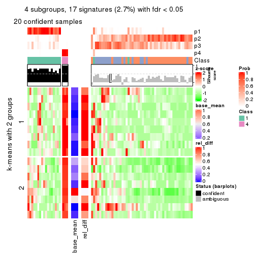
get_signatures(res, k = 5)
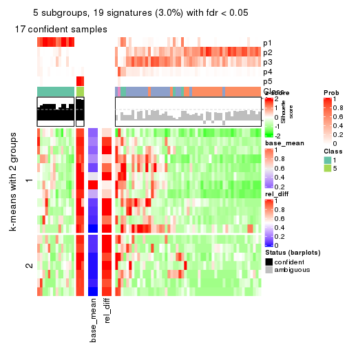
get_signatures(res, k = 6)
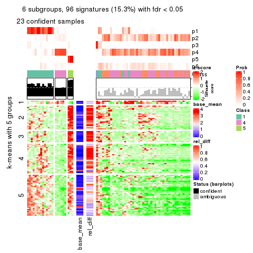
Signature heatmaps where rows are not scaled:
get_signatures(res, k = 2, scale_rows = FALSE)
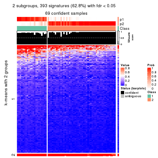
get_signatures(res, k = 3, scale_rows = FALSE)
get_signatures(res, k = 4, scale_rows = FALSE)
get_signatures(res, k = 5, scale_rows = FALSE)
get_signatures(res, k = 6, scale_rows = FALSE)
Compare the overlap of signatures from different k:
compare_signatures(res)
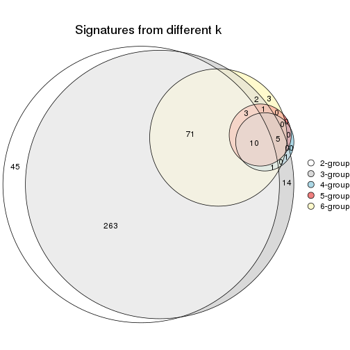
get_signature() returns a data frame invisibly. TO get the list of signatures, the function
call should be assigned to a variable explicitly. In following code, if plot argument is set
to FALSE, no heatmap is plotted while only the differential analysis is performed.
# code only for demonstration
tb = get_signature(res, k = ..., plot = FALSE)
An example of the output of tb is:
#>   which_row         fdr    mean_1    mean_2 scaled_mean_1 scaled_mean_2 km
#> 1        38 0.042760348  8.373488  9.131774    -0.5533452     0.5164555  1
#> 2        40 0.018707592  7.106213  8.469186    -0.6173731     0.5762149  1
#> 3        55 0.019134737 10.221463 11.207825    -0.6159697     0.5749050  1
#> 4        59 0.006059896  5.921854  7.869574    -0.6899429     0.6439467  1
#> 5        60 0.018055526  8.928898 10.211722    -0.6204761     0.5791110  1
#> 6        98 0.009384629 15.714769 14.887706     0.6635654    -0.6193277  2
...
The columns in tb are:
which_row: row indices corresponding to the input matrix.fdr: FDR for the differential test. mean_x: The mean value in group x.scaled_mean_x: The mean value in group x after rows are scaled.km: Row groups if k-means clustering is applied to rows.UMAP plot which shows how samples are separated.
dimension_reduction(res, k = 2, method = "UMAP")
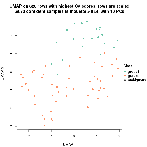
dimension_reduction(res, k = 3, method = "UMAP")
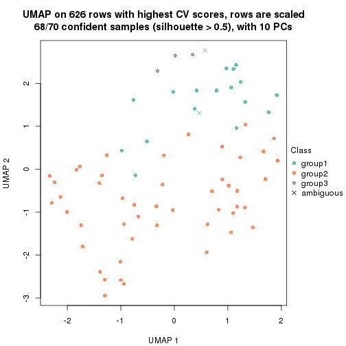
dimension_reduction(res, k = 4, method = "UMAP")
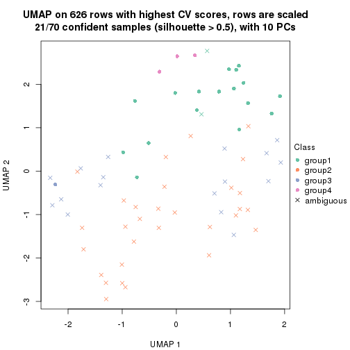
dimension_reduction(res, k = 5, method = "UMAP")
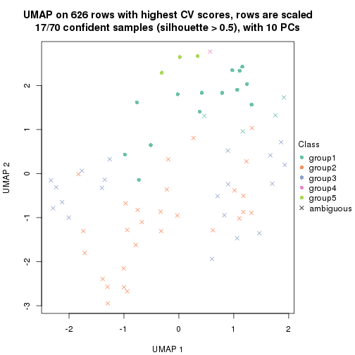
dimension_reduction(res, k = 6, method = "UMAP")
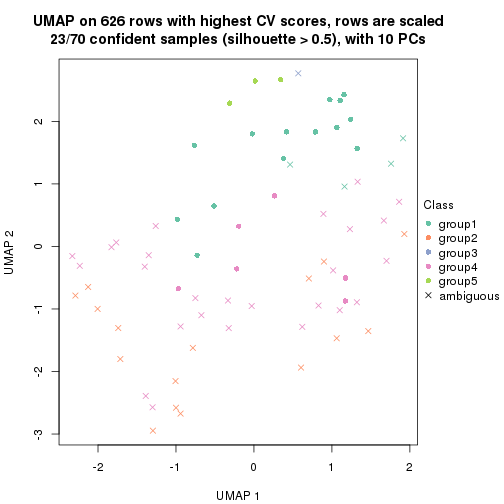
Following heatmap shows how subgroups are split when increasing k:
collect_classes(res)
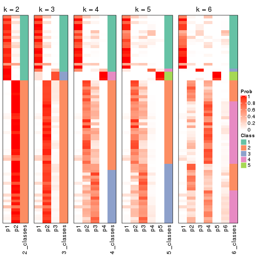
If matrix rows can be associated to genes, consider to use functional_enrichment(res,
...) to perform function enrichment for the signature genes. See this vignette for more detailed explanations.
The object with results only for a single top-value method and a single partition method can be extracted as:
res = res_list["CV", "mclust"]
# you can also extract it by
# res = res_list["CV:mclust"]
A summary of res and all the functions that can be applied to it:
res
#> A 'ConsensusPartition' object with k = 2, 3, 4, 5, 6.
#>   On a matrix with 626 rows and 70 columns.
#>   Top rows (63, 126, 188, 250, 313) are extracted by 'CV' method.
#>   Subgroups are detected by 'mclust' method.
#>   Performed in total 1250 partitions by row resampling.
#>   Best k for subgroups seems to be 2.
#>
#> Following methods can be applied to this 'ConsensusPartition' object:
#>  [1] "cola_report"             "collect_classes"         "collect_plots"
#>  [4] "collect_stats"           "colnames"                "compare_signatures"
#>  [7] "consensus_heatmap"       "dimension_reduction"     "functional_enrichment"
#> [10] "get_anno_col"            "get_anno"                "get_classes"
#> [13] "get_consensus"           "get_matrix"              "get_membership"
#> [16] "get_param"               "get_signatures"          "get_stats"
#> [19] "is_best_k"               "is_stable_k"             "membership_heatmap"
#> [22] "ncol"                    "nrow"                    "plot_ecdf"
#> [25] "rownames"                "select_partition_number" "show"
#> [28] "suggest_best_k"          "test_to_known_factors"
collect_plots() function collects all the plots made from res for all k (number of partitions)
into one single page to provide an easy and fast comparison between different k.
collect_plots(res)
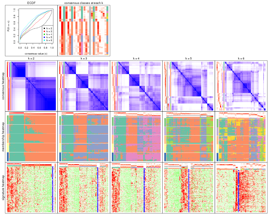
The plots are:
k and the heatmap of
predicted classes for each k.k.k.k.All the plots in panels can be made by individual functions and they are plotted later in this section.
select_partition_number() produces several plots showing different
statistics for choosing “optimized” k. There are following statistics:
k;k, the area increased is defined as \(A_k - A_{k-1}\).The detailed explanations of these statistics can be found in the cola vignette.
Generally speaking, lower PAC score, higher mean silhouette score or higher
concordance corresponds to better partition. Rand index and Jaccard index
measure how similar the current partition is compared to partition with k-1.
If they are too similar, we won't accept k is better than k-1.
select_partition_number(res)

The numeric values for all these statistics can be obtained by get_stats().
get_stats(res)
#>   k 1-PAC mean_silhouette concordance area_increased  Rand Jaccard
#> 2 2 0.533           0.841       0.908         0.4482 0.563   0.563
#> 3 3 0.311           0.605       0.728         0.3049 0.692   0.494
#> 4 4 0.281           0.537       0.653         0.1325 0.865   0.640
#> 5 5 0.340           0.394       0.596         0.0424 0.735   0.419
#> 6 6 0.421           0.389       0.612         0.0636 0.841   0.609
suggest_best_k() suggests the best \(k\) based on these statistics. The rules are as follows:
suggest_best_k(res)
#> [1] 2
Following shows the table of the partitions (You need to click the show/hide
code output link to see it). The membership matrix (columns with name p*)
is inferred by
clue::cl_consensus()
function with the SE method. Basically the value in the membership matrix
represents the probability to belong to a certain group. The finall class
label for an item is determined with the group with highest probability it
belongs to.
In get_classes() function, the entropy is calculated from the membership
matrix and the silhouette score is calculated from the consensus matrix.
cbind(get_classes(res, k = 2), get_membership(res, k = 2))
#>           class entropy silhouette    p1    p2
#> SRR837437     2  0.0000      0.886 0.000 1.000
#> SRR837438     2  0.3879      0.884 0.076 0.924
#> SRR837439     2  0.0000      0.886 0.000 1.000
#> SRR837440     2  0.0672      0.887 0.008 0.992
#> SRR837441     2  0.0000      0.886 0.000 1.000
#> SRR837442     2  0.0000      0.886 0.000 1.000
#> SRR837443     2  0.0000      0.886 0.000 1.000
#> SRR837444     2  0.2423      0.890 0.040 0.960
#> SRR837445     2  0.2948      0.888 0.052 0.948
#> SRR837446     2  0.4431      0.878 0.092 0.908
#> SRR837447     1  0.0938      0.928 0.988 0.012
#> SRR837448     1  0.0000      0.932 1.000 0.000
#> SRR837449     1  0.6343      0.811 0.840 0.160
#> SRR837450     1  0.0000      0.932 1.000 0.000
#> SRR837451     2  0.0000      0.886 0.000 1.000
#> SRR837452     2  0.1414      0.888 0.020 0.980
#> SRR837453     2  0.0000      0.886 0.000 1.000
#> SRR837454     2  0.0000      0.886 0.000 1.000
#> SRR837455     1  0.0000      0.932 1.000 0.000
#> SRR837456     1  0.0000      0.932 1.000 0.000
#> SRR837457     2  0.0000      0.886 0.000 1.000
#> SRR837458     1  0.0000      0.932 1.000 0.000
#> SRR837459     2  0.0000      0.886 0.000 1.000
#> SRR837460     2  0.0376      0.887 0.004 0.996
#> SRR837461     2  0.4562      0.879 0.096 0.904
#> SRR837462     2  0.8555      0.725 0.280 0.720
#> SRR837463     2  0.9954      0.322 0.460 0.540
#> SRR837464     2  0.8386      0.739 0.268 0.732
#> SRR837465     2  0.7883      0.781 0.236 0.764
#> SRR837466     1  0.0000      0.932 1.000 0.000
#> SRR837467     2  0.0376      0.885 0.004 0.996
#> SRR837468     1  0.0000      0.932 1.000 0.000
#> SRR837469     1  0.0000      0.932 1.000 0.000
#> SRR837470     1  0.0000      0.932 1.000 0.000
#> SRR837471     2  0.3584      0.885 0.068 0.932
#> SRR837472     2  0.4298      0.879 0.088 0.912
#> SRR837473     1  0.8909      0.523 0.692 0.308
#> SRR837474     2  0.1843      0.889 0.028 0.972
#> SRR837475     2  0.4161      0.881 0.084 0.916
#> SRR837476     2  0.0000      0.886 0.000 1.000
#> SRR837477     1  0.8608      0.554 0.716 0.284
#> SRR837478     2  0.8555      0.725 0.280 0.720
#> SRR837479     2  0.7602      0.792 0.220 0.780
#> SRR837480     2  0.7376      0.802 0.208 0.792
#> SRR837481     2  0.6712      0.830 0.176 0.824
#> SRR837482     2  0.5737      0.855 0.136 0.864
#> SRR837483     1  0.0000      0.932 1.000 0.000
#> SRR837484     2  0.5629      0.860 0.132 0.868
#> SRR837485     2  0.6712      0.831 0.176 0.824
#> SRR837486     1  0.1843      0.920 0.972 0.028
#> SRR837487     2  0.0376      0.887 0.004 0.996
#> SRR837488     2  0.0376      0.887 0.004 0.996
#> SRR837489     2  0.2603      0.889 0.044 0.956
#> SRR837490     2  0.0000      0.886 0.000 1.000
#> SRR837491     2  0.4939      0.871 0.108 0.892
#> SRR837492     1  0.0000      0.932 1.000 0.000
#> SRR837493     2  0.3431      0.886 0.064 0.936
#> SRR837494     2  0.0000      0.886 0.000 1.000
#> SRR837495     2  0.8207      0.752 0.256 0.744
#> SRR837496     1  0.0000      0.932 1.000 0.000
#> SRR837497     1  0.0938      0.928 0.988 0.012
#> SRR837498     1  0.3879      0.890 0.924 0.076
#> SRR837499     1  0.5629      0.842 0.868 0.132
#> SRR837500     1  0.6712      0.791 0.824 0.176
#> SRR837501     2  0.9866      0.424 0.432 0.568
#> SRR837502     2  0.7815      0.735 0.232 0.768
#> SRR837503     1  0.2778      0.910 0.952 0.048
#> SRR837504     2  0.2423      0.889 0.040 0.960
#> SRR837505     2  0.9710      0.517 0.400 0.600
#> SRR837506     2  0.9552      0.565 0.376 0.624
cbind(get_classes(res, k = 3), get_membership(res, k = 3))
#>           class entropy silhouette    p1    p2    p3
#> SRR837437     2  0.1860      0.798 0.000 0.948 0.052
#> SRR837438     3  0.7271      0.654 0.040 0.352 0.608
#> SRR837439     2  0.1860      0.797 0.000 0.948 0.052
#> SRR837440     2  0.6235     -0.185 0.000 0.564 0.436
#> SRR837441     2  0.1753      0.797 0.000 0.952 0.048
#> SRR837442     2  0.1860      0.797 0.000 0.948 0.052
#> SRR837443     2  0.2165      0.795 0.000 0.936 0.064
#> SRR837444     3  0.5810      0.631 0.000 0.336 0.664
#> SRR837445     3  0.6204      0.539 0.000 0.424 0.576
#> SRR837446     3  0.6501      0.656 0.020 0.316 0.664
#> SRR837447     1  0.2939      0.800 0.916 0.012 0.072
#> SRR837448     1  0.1753      0.800 0.952 0.000 0.048
#> SRR837449     1  0.8020      0.419 0.604 0.088 0.308
#> SRR837450     1  0.1753      0.800 0.952 0.000 0.048
#> SRR837451     2  0.0424      0.780 0.000 0.992 0.008
#> SRR837452     3  0.6483      0.506 0.004 0.452 0.544
#> SRR837453     2  0.0592      0.782 0.000 0.988 0.012
#> SRR837454     2  0.0747      0.787 0.000 0.984 0.016
#> SRR837455     1  0.2269      0.802 0.944 0.016 0.040
#> SRR837456     1  0.1950      0.804 0.952 0.008 0.040
#> SRR837457     2  0.0892      0.786 0.000 0.980 0.020
#> SRR837458     1  0.1753      0.800 0.952 0.000 0.048
#> SRR837459     2  0.2711      0.760 0.000 0.912 0.088
#> SRR837460     2  0.1163      0.784 0.000 0.972 0.028
#> SRR837461     3  0.7346      0.643 0.040 0.368 0.592
#> SRR837462     3  0.8513      0.691 0.140 0.264 0.596
#> SRR837463     3  0.8595      0.680 0.180 0.216 0.604
#> SRR837464     3  0.8561      0.690 0.156 0.244 0.600
#> SRR837465     3  0.8435      0.696 0.132 0.268 0.600
#> SRR837466     1  0.1753      0.800 0.952 0.000 0.048
#> SRR837467     2  0.5325      0.564 0.004 0.748 0.248
#> SRR837468     1  0.5435      0.714 0.808 0.048 0.144
#> SRR837469     1  0.1289      0.804 0.968 0.000 0.032
#> SRR837470     1  0.1289      0.804 0.968 0.000 0.032
#> SRR837471     3  0.6565      0.552 0.008 0.416 0.576
#> SRR837472     3  0.6489      0.476 0.004 0.456 0.540
#> SRR837473     3  0.7106      0.463 0.232 0.072 0.696
#> SRR837474     2  0.6280     -0.255 0.000 0.540 0.460
#> SRR837475     3  0.6386      0.540 0.004 0.412 0.584
#> SRR837476     2  0.4062      0.704 0.000 0.836 0.164
#> SRR837477     3  0.7246      0.408 0.276 0.060 0.664
#> SRR837478     3  0.6354      0.676 0.056 0.196 0.748
#> SRR837479     3  0.5777      0.676 0.052 0.160 0.788
#> SRR837480     3  0.6319      0.677 0.040 0.228 0.732
#> SRR837481     3  0.5688      0.681 0.044 0.168 0.788
#> SRR837482     3  0.6264      0.680 0.032 0.244 0.724
#> SRR837483     1  0.1753      0.802 0.952 0.000 0.048
#> SRR837484     3  0.7580      0.644 0.056 0.340 0.604
#> SRR837485     3  0.7015      0.683 0.064 0.240 0.696
#> SRR837486     1  0.7699      0.277 0.560 0.052 0.388
#> SRR837487     2  0.5216      0.568 0.000 0.740 0.260
#> SRR837488     2  0.2959      0.767 0.000 0.900 0.100
#> SRR837489     3  0.6754      0.539 0.012 0.432 0.556
#> SRR837490     2  0.4654      0.652 0.000 0.792 0.208
#> SRR837491     3  0.7299      0.585 0.032 0.412 0.556
#> SRR837492     1  0.7379      0.472 0.616 0.048 0.336
#> SRR837493     3  0.7080      0.598 0.024 0.412 0.564
#> SRR837494     2  0.1289      0.794 0.000 0.968 0.032
#> SRR837495     3  0.6443      0.658 0.040 0.240 0.720
#> SRR837496     1  0.2066      0.802 0.940 0.000 0.060
#> SRR837497     1  0.5431      0.642 0.716 0.000 0.284
#> SRR837498     1  0.8326      0.031 0.488 0.080 0.432
#> SRR837499     3  0.7828     -0.210 0.448 0.052 0.500
#> SRR837500     3  0.8350      0.123 0.380 0.088 0.532
#> SRR837501     3  0.7695      0.608 0.200 0.124 0.676
#> SRR837502     3  0.7059      0.668 0.092 0.192 0.716
#> SRR837503     1  0.6398      0.491 0.580 0.004 0.416
#> SRR837504     2  0.6451     -0.147 0.004 0.560 0.436
#> SRR837505     3  0.7413      0.589 0.204 0.104 0.692
#> SRR837506     3  0.7999      0.634 0.196 0.148 0.656
cbind(get_classes(res, k = 4), get_membership(res, k = 4))
#>           class entropy silhouette    p1    p2    p3    p4
#> SRR837437     2   0.461     0.8437 0.000 0.692 0.004 0.304
#> SRR837438     4   0.288     0.5514 0.008 0.060 0.028 0.904
#> SRR837439     2   0.453     0.8512 0.000 0.704 0.004 0.292
#> SRR837440     4   0.756    -0.1266 0.000 0.328 0.208 0.464
#> SRR837441     2   0.453     0.8461 0.000 0.704 0.004 0.292
#> SRR837442     2   0.465     0.8434 0.000 0.684 0.004 0.312
#> SRR837443     2   0.491     0.8397 0.000 0.676 0.012 0.312
#> SRR837444     4   0.362     0.5395 0.000 0.076 0.064 0.860
#> SRR837445     4   0.376     0.5393 0.000 0.152 0.020 0.828
#> SRR837446     3   0.672     0.5176 0.004 0.076 0.476 0.444
#> SRR837447     1   0.319     0.7382 0.896 0.040 0.020 0.044
#> SRR837448     1   0.411     0.7274 0.812 0.032 0.156 0.000
#> SRR837449     1   0.741     0.2146 0.472 0.008 0.132 0.388
#> SRR837450     1   0.415     0.7285 0.812 0.036 0.152 0.000
#> SRR837451     2   0.505     0.8527 0.000 0.704 0.028 0.268
#> SRR837452     4   0.538     0.4635 0.000 0.120 0.136 0.744
#> SRR837453     2   0.539     0.8523 0.000 0.688 0.044 0.268
#> SRR837454     2   0.474     0.8579 0.000 0.704 0.012 0.284
#> SRR837455     1   0.320     0.7295 0.888 0.032 0.008 0.072
#> SRR837456     1   0.295     0.7326 0.900 0.028 0.008 0.064
#> SRR837457     2   0.537     0.8487 0.000 0.692 0.044 0.264
#> SRR837458     1   0.346     0.7408 0.860 0.020 0.116 0.004
#> SRR837459     2   0.544     0.8478 0.000 0.672 0.040 0.288
#> SRR837460     2   0.550     0.8430 0.000 0.680 0.048 0.272
#> SRR837461     4   0.764     0.0827 0.036 0.124 0.280 0.560
#> SRR837462     4   0.721    -0.0738 0.096 0.020 0.336 0.548
#> SRR837463     4   0.697     0.1594 0.108 0.020 0.256 0.616
#> SRR837464     4   0.736    -0.0667 0.104 0.024 0.324 0.548
#> SRR837465     4   0.659     0.2550 0.092 0.020 0.232 0.656
#> SRR837466     1   0.411     0.7274 0.812 0.032 0.156 0.000
#> SRR837467     2   0.678     0.5779 0.004 0.464 0.080 0.452
#> SRR837468     1   0.676     0.6566 0.676 0.148 0.144 0.032
#> SRR837469     1   0.443     0.7253 0.796 0.168 0.032 0.004
#> SRR837470     1   0.433     0.7272 0.800 0.168 0.028 0.004
#> SRR837471     4   0.397     0.5148 0.000 0.180 0.016 0.804
#> SRR837472     4   0.434     0.5103 0.000 0.168 0.036 0.796
#> SRR837473     4   0.582     0.3681 0.136 0.032 0.084 0.748
#> SRR837474     4   0.453     0.3710 0.000 0.240 0.016 0.744
#> SRR837475     4   0.362     0.5489 0.000 0.112 0.036 0.852
#> SRR837476     2   0.541     0.7371 0.000 0.576 0.016 0.408
#> SRR837477     4   0.777     0.1215 0.240 0.032 0.168 0.560
#> SRR837478     4   0.681    -0.1362 0.056 0.028 0.336 0.580
#> SRR837479     3   0.639     0.6587 0.044 0.012 0.552 0.392
#> SRR837480     4   0.578     0.2265 0.020 0.044 0.232 0.704
#> SRR837481     3   0.593     0.6679 0.020 0.012 0.560 0.408
#> SRR837482     3   0.620     0.6508 0.008 0.040 0.560 0.392
#> SRR837483     1   0.361     0.7394 0.844 0.024 0.132 0.000
#> SRR837484     3   0.657     0.6221 0.012 0.056 0.552 0.380
#> SRR837485     3   0.599     0.7121 0.020 0.024 0.620 0.336
#> SRR837486     1   0.767     0.2121 0.548 0.020 0.252 0.180
#> SRR837487     2   0.758     0.4476 0.000 0.424 0.196 0.380
#> SRR837488     2   0.630     0.8020 0.000 0.600 0.080 0.320
#> SRR837489     4   0.423     0.5417 0.004 0.124 0.048 0.824
#> SRR837490     2   0.559     0.6070 0.000 0.520 0.020 0.460
#> SRR837491     4   0.443     0.5419 0.008 0.156 0.032 0.804
#> SRR837492     1   0.671     0.4322 0.580 0.020 0.060 0.340
#> SRR837493     4   0.402     0.5455 0.004 0.104 0.052 0.840
#> SRR837494     2   0.486     0.8586 0.000 0.700 0.016 0.284
#> SRR837495     4   0.364     0.5148 0.024 0.052 0.048 0.876
#> SRR837496     1   0.356     0.7345 0.876 0.020 0.072 0.032
#> SRR837497     1   0.607     0.5934 0.684 0.020 0.056 0.240
#> SRR837498     1   0.669     0.2319 0.508 0.004 0.076 0.412
#> SRR837499     4   0.674     0.1081 0.332 0.020 0.064 0.584
#> SRR837500     4   0.629     0.2025 0.308 0.012 0.056 0.624
#> SRR837501     3   0.649     0.6714 0.144 0.000 0.636 0.220
#> SRR837502     4   0.352     0.4968 0.060 0.020 0.040 0.880
#> SRR837503     1   0.729     0.4078 0.528 0.032 0.076 0.364
#> SRR837504     4   0.762    -0.2041 0.000 0.208 0.360 0.432
#> SRR837505     3   0.663     0.6569 0.160 0.000 0.624 0.216
#> SRR837506     3   0.689     0.6816 0.144 0.008 0.616 0.232
cbind(get_classes(res, k = 5), get_membership(res, k = 5))
#>           class entropy silhouette    p1    p2    p3 p4    p5
#> SRR837437     2   0.460     0.5402 0.000 0.600 0.016 NA 0.000
#> SRR837438     2   0.464     0.4301 0.152 0.764 0.020 NA 0.000
#> SRR837439     2   0.452     0.5377 0.000 0.600 0.012 NA 0.000
#> SRR837440     2   0.555     0.4360 0.016 0.680 0.188 NA 0.000
#> SRR837441     2   0.459     0.5409 0.000 0.604 0.016 NA 0.000
#> SRR837442     2   0.405     0.5489 0.000 0.644 0.000 NA 0.000
#> SRR837443     2   0.454     0.5456 0.000 0.620 0.016 NA 0.000
#> SRR837444     2   0.468     0.4171 0.172 0.756 0.040 NA 0.000
#> SRR837445     2   0.377     0.4793 0.104 0.828 0.012 NA 0.000
#> SRR837446     2   0.648    -0.2661 0.076 0.480 0.404 NA 0.000
#> SRR837447     5   0.742     0.5457 0.184 0.004 0.040 NA 0.420
#> SRR837448     5   0.137     0.5393 0.008 0.000 0.008 NA 0.956
#> SRR837449     1   0.824     0.5319 0.528 0.172 0.120 NA 0.080
#> SRR837450     5   0.235     0.5540 0.060 0.000 0.004 NA 0.908
#> SRR837451     2   0.433     0.5260 0.000 0.596 0.004 NA 0.000
#> SRR837452     2   0.347     0.4551 0.040 0.840 0.112 NA 0.000
#> SRR837453     2   0.434     0.5229 0.000 0.592 0.004 NA 0.000
#> SRR837454     2   0.420     0.5275 0.000 0.592 0.000 NA 0.000
#> SRR837455     5   0.781     0.5343 0.184 0.016 0.048 NA 0.408
#> SRR837456     5   0.774     0.5355 0.188 0.012 0.048 NA 0.408
#> SRR837457     2   0.444     0.5241 0.000 0.596 0.008 NA 0.000
#> SRR837458     5   0.605     0.6198 0.144 0.000 0.028 NA 0.644
#> SRR837459     2   0.432     0.5275 0.000 0.600 0.004 NA 0.000
#> SRR837460     2   0.434     0.5241 0.000 0.592 0.004 NA 0.000
#> SRR837461     2   0.651     0.2552 0.060 0.604 0.232 NA 0.000
#> SRR837462     2   0.803    -0.1629 0.200 0.400 0.312 NA 0.008
#> SRR837463     2   0.837    -0.1364 0.228 0.396 0.264 NA 0.016
#> SRR837464     2   0.821    -0.1651 0.180 0.408 0.316 NA 0.028
#> SRR837465     2   0.826     0.0329 0.216 0.472 0.188 NA 0.032
#> SRR837466     5   0.115     0.5453 0.008 0.000 0.004 NA 0.964
#> SRR837467     2   0.446     0.5470 0.004 0.748 0.056 NA 0.000
#> SRR837468     3   0.732    -0.5940 0.128 0.000 0.424 NA 0.380
#> SRR837469     5   0.789     0.5453 0.144 0.000 0.256 NA 0.452
#> SRR837470     5   0.784     0.5589 0.148 0.000 0.244 NA 0.464
#> SRR837471     2   0.375     0.4838 0.072 0.832 0.012 NA 0.000
#> SRR837472     2   0.318     0.4880 0.068 0.872 0.024 NA 0.000
#> SRR837473     1   0.544     0.5581 0.688 0.232 0.012 NA 0.044
#> SRR837474     2   0.299     0.5259 0.024 0.872 0.012 NA 0.000
#> SRR837475     2   0.439     0.4354 0.132 0.784 0.016 NA 0.000
#> SRR837476     2   0.377     0.5624 0.000 0.728 0.004 NA 0.000
#> SRR837477     1   0.650     0.5353 0.660 0.164 0.076 NA 0.080
#> SRR837478     2   0.707    -0.2349 0.288 0.404 0.296 NA 0.000
#> SRR837479     3   0.649     0.4592 0.124 0.348 0.512 NA 0.004
#> SRR837480     2   0.679     0.0223 0.240 0.532 0.208 NA 0.004
#> SRR837481     3   0.641     0.4811 0.124 0.356 0.508 NA 0.004
#> SRR837482     3   0.586     0.4437 0.068 0.400 0.520 NA 0.000
#> SRR837483     5   0.534     0.5373 0.244 0.000 0.056 NA 0.676
#> SRR837484     3   0.569     0.2988 0.036 0.452 0.492 NA 0.004
#> SRR837485     3   0.494     0.4797 0.016 0.376 0.596 NA 0.000
#> SRR837486     3   0.820    -0.1937 0.120 0.088 0.444 NA 0.308
#> SRR837487     2   0.598     0.4533 0.012 0.628 0.188 NA 0.000
#> SRR837488     2   0.502     0.5355 0.004 0.628 0.040 NA 0.000
#> SRR837489     2   0.284     0.4921 0.092 0.876 0.004 NA 0.000
#> SRR837490     2   0.340     0.5546 0.000 0.780 0.004 NA 0.000
#> SRR837491     2   0.418     0.4836 0.112 0.796 0.008 NA 0.000
#> SRR837492     1   0.594     0.3956 0.636 0.036 0.040 NA 0.272
#> SRR837493     2   0.364     0.4777 0.100 0.840 0.036 NA 0.000
#> SRR837494     2   0.452     0.5310 0.000 0.600 0.012 NA 0.000
#> SRR837495     2   0.501     0.2741 0.332 0.632 0.008 NA 0.004
#> SRR837496     1   0.547     0.0150 0.564 0.000 0.028 NA 0.384
#> SRR837497     1   0.616     0.2681 0.592 0.024 0.044 NA 0.316
#> SRR837498     1   0.896     0.3337 0.448 0.140 0.136 NA 0.176
#> SRR837499     1   0.618     0.5934 0.664 0.184 0.008 NA 0.052
#> SRR837500     1   0.631     0.5900 0.648 0.200 0.008 NA 0.052
#> SRR837501     3   0.496     0.5669 0.020 0.176 0.740 NA 0.060
#> SRR837502     2   0.550     0.0841 0.372 0.572 0.008 NA 0.004
#> SRR837503     1   0.444     0.5644 0.796 0.056 0.020 NA 0.120
#> SRR837504     2   0.542     0.2045 0.024 0.616 0.324 NA 0.000
#> SRR837505     3   0.542     0.5798 0.028 0.212 0.696 NA 0.060
#> SRR837506     3   0.566     0.5740 0.028 0.248 0.660 NA 0.060
cbind(get_classes(res, k = 6), get_membership(res, k = 6))
#>           class entropy silhouette    p1    p2    p3    p4    p5    p6
#> SRR837437     2  0.2312     0.6572 0.000 0.876 0.012 0.000 0.000 0.112
#> SRR837438     2  0.6854     0.4274 0.140 0.416 0.032 0.032 0.000 0.380
#> SRR837439     2  0.1657     0.6511 0.000 0.928 0.016 0.000 0.000 0.056
#> SRR837440     2  0.5294     0.4998 0.020 0.652 0.232 0.008 0.000 0.088
#> SRR837441     2  0.2006     0.6530 0.000 0.904 0.016 0.000 0.000 0.080
#> SRR837442     2  0.2006     0.6664 0.000 0.892 0.004 0.000 0.000 0.104
#> SRR837443     2  0.2218     0.6609 0.000 0.884 0.012 0.000 0.000 0.104
#> SRR837444     2  0.6642     0.4847 0.208 0.464 0.032 0.008 0.000 0.288
#> SRR837445     2  0.5805     0.5230 0.168 0.484 0.004 0.000 0.000 0.344
#> SRR837446     3  0.6932     0.3059 0.068 0.308 0.484 0.028 0.000 0.112
#> SRR837447     6  0.8044     0.1184 0.172 0.008 0.012 0.288 0.204 0.316
#> SRR837448     5  0.0260     0.6800 0.008 0.000 0.000 0.000 0.992 0.000
#> SRR837449     1  0.7171     0.2387 0.512 0.040 0.096 0.052 0.020 0.280
#> SRR837450     5  0.1760     0.6890 0.048 0.000 0.004 0.020 0.928 0.000
#> SRR837451     2  0.1536     0.6399 0.000 0.940 0.004 0.016 0.000 0.040
#> SRR837452     2  0.6537     0.5430 0.108 0.540 0.100 0.004 0.000 0.248
#> SRR837453     2  0.1332     0.6457 0.000 0.952 0.012 0.008 0.000 0.028
#> SRR837454     2  0.1332     0.6460 0.000 0.952 0.008 0.012 0.000 0.028
#> SRR837455     6  0.7336     0.2628 0.108 0.000 0.008 0.280 0.188 0.416
#> SRR837456     6  0.7354     0.2576 0.108 0.000 0.008 0.280 0.192 0.412
#> SRR837457     2  0.1894     0.6432 0.004 0.928 0.016 0.012 0.000 0.040
#> SRR837458     5  0.7184     0.2127 0.108 0.000 0.008 0.216 0.468 0.200
#> SRR837459     2  0.1908     0.6416 0.000 0.924 0.020 0.012 0.000 0.044
#> SRR837460     2  0.1932     0.6386 0.000 0.924 0.016 0.020 0.000 0.040
#> SRR837461     2  0.7304     0.2411 0.028 0.504 0.228 0.124 0.004 0.112
#> SRR837462     3  0.8090     0.1872 0.048 0.232 0.316 0.296 0.000 0.108
#> SRR837463     4  0.8298    -0.3478 0.060 0.224 0.236 0.340 0.000 0.140
#> SRR837464     3  0.8088     0.2041 0.052 0.244 0.328 0.276 0.000 0.100
#> SRR837465     2  0.8165    -0.1049 0.056 0.328 0.156 0.312 0.000 0.148
#> SRR837466     5  0.0951     0.6854 0.008 0.000 0.000 0.020 0.968 0.004
#> SRR837467     2  0.4763     0.6444 0.028 0.744 0.064 0.020 0.000 0.144
#> SRR837468     4  0.6853     0.2550 0.112 0.000 0.200 0.500 0.188 0.000
#> SRR837469     4  0.5044     0.2747 0.120 0.000 0.012 0.664 0.204 0.000
#> SRR837470     4  0.5327     0.2467 0.120 0.000 0.012 0.636 0.228 0.004
#> SRR837471     2  0.6053     0.5169 0.152 0.476 0.008 0.008 0.000 0.356
#> SRR837472     2  0.6295     0.5371 0.148 0.516 0.024 0.012 0.000 0.300
#> SRR837473     1  0.2843     0.4055 0.860 0.028 0.004 0.004 0.000 0.104
#> SRR837474     2  0.5258     0.5932 0.080 0.584 0.008 0.004 0.000 0.324
#> SRR837475     2  0.6727     0.4484 0.216 0.412 0.024 0.012 0.000 0.336
#> SRR837476     2  0.2605     0.6739 0.020 0.876 0.012 0.000 0.000 0.092
#> SRR837477     1  0.2883     0.4105 0.888 0.024 0.032 0.008 0.036 0.012
#> SRR837478     1  0.7032    -0.2532 0.388 0.256 0.304 0.000 0.012 0.040
#> SRR837479     3  0.5912     0.4862 0.204 0.100 0.636 0.016 0.004 0.040
#> SRR837480     1  0.7509    -0.1635 0.360 0.292 0.212 0.000 0.004 0.132
#> SRR837481     3  0.6664     0.5290 0.168 0.148 0.584 0.060 0.000 0.040
#> SRR837482     3  0.5833     0.5573 0.036 0.172 0.664 0.072 0.000 0.056
#> SRR837483     5  0.5937     0.4040 0.240 0.000 0.024 0.144 0.584 0.008
#> SRR837484     3  0.6011     0.3457 0.044 0.328 0.552 0.028 0.000 0.048
#> SRR837485     3  0.5128     0.5338 0.040 0.240 0.672 0.008 0.004 0.036
#> SRR837486     3  0.7017    -0.3393 0.120 0.000 0.456 0.264 0.160 0.000
#> SRR837487     2  0.4762     0.5834 0.012 0.716 0.172 0.008 0.000 0.092
#> SRR837488     2  0.2898     0.6505 0.016 0.868 0.056 0.000 0.000 0.060
#> SRR837489     2  0.6025     0.5535 0.124 0.524 0.020 0.008 0.000 0.324
#> SRR837490     2  0.3861     0.6558 0.028 0.744 0.008 0.000 0.000 0.220
#> SRR837491     2  0.5808     0.5355 0.088 0.496 0.004 0.024 0.000 0.388
#> SRR837492     1  0.3950     0.2821 0.780 0.004 0.004 0.056 0.152 0.004
#> SRR837493     2  0.6457     0.5266 0.096 0.512 0.048 0.020 0.000 0.324
#> SRR837494     2  0.1173     0.6482 0.000 0.960 0.008 0.016 0.000 0.016
#> SRR837495     1  0.6170    -0.2120 0.420 0.348 0.008 0.000 0.000 0.224
#> SRR837496     1  0.4937     0.1465 0.684 0.000 0.004 0.116 0.188 0.008
#> SRR837497     1  0.5794     0.2146 0.672 0.004 0.040 0.100 0.156 0.028
#> SRR837498     1  0.8902    -0.0841 0.348 0.072 0.076 0.260 0.072 0.172
#> SRR837499     1  0.5248     0.3364 0.636 0.036 0.004 0.028 0.012 0.284
#> SRR837500     1  0.5575     0.3297 0.616 0.060 0.004 0.028 0.012 0.280
#> SRR837501     3  0.3528     0.4129 0.028 0.028 0.852 0.052 0.036 0.004
#> SRR837502     6  0.6839    -0.3458 0.368 0.220 0.020 0.020 0.000 0.372
#> SRR837503     1  0.1514     0.3954 0.944 0.000 0.004 0.004 0.036 0.012
#> SRR837504     2  0.5711     0.2689 0.016 0.536 0.356 0.012 0.000 0.080
#> SRR837505     3  0.3548     0.4412 0.036 0.032 0.856 0.028 0.036 0.012
#> SRR837506     3  0.5225     0.5070 0.052 0.140 0.728 0.028 0.044 0.008
Heatmaps for the consensus matrix. It visualizes the probability of two samples to be in a same group.
consensus_heatmap(res, k = 2)
consensus_heatmap(res, k = 3)
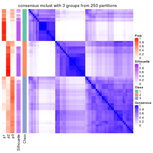
consensus_heatmap(res, k = 4)
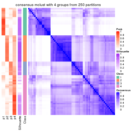
consensus_heatmap(res, k = 5)
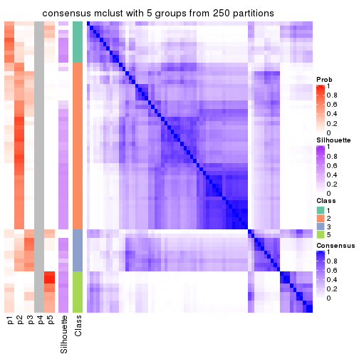
consensus_heatmap(res, k = 6)
Heatmaps for the membership of samples in all partitions to see how consistent they are:
membership_heatmap(res, k = 2)
membership_heatmap(res, k = 3)
membership_heatmap(res, k = 4)
membership_heatmap(res, k = 5)
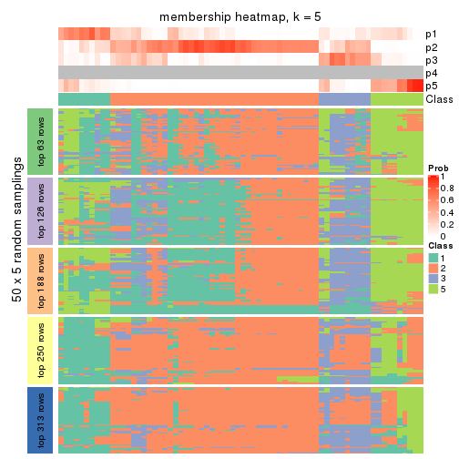
membership_heatmap(res, k = 6)
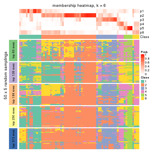
As soon as we have had the classes for columns, we can look for signatures which are significantly different between classes which can be candidate marks for certain classes. Following are the heatmaps for signatures.
Signature heatmaps where rows are scaled:
get_signatures(res, k = 2)
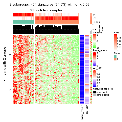
get_signatures(res, k = 3)
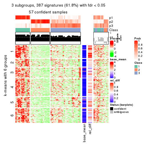
get_signatures(res, k = 4)
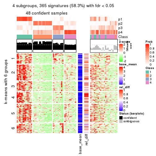
get_signatures(res, k = 5)
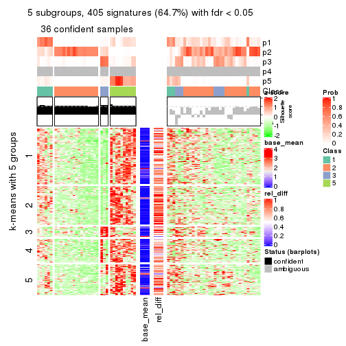
get_signatures(res, k = 6)
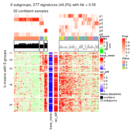
Signature heatmaps where rows are not scaled:
get_signatures(res, k = 2, scale_rows = FALSE)
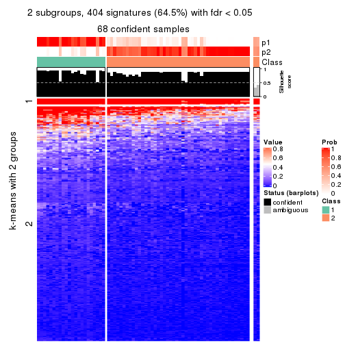
get_signatures(res, k = 3, scale_rows = FALSE)
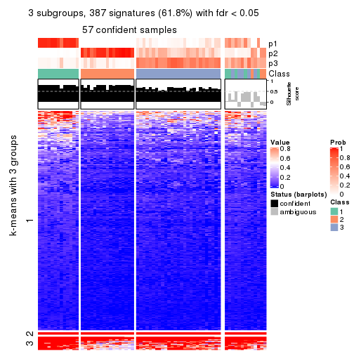
get_signatures(res, k = 4, scale_rows = FALSE)
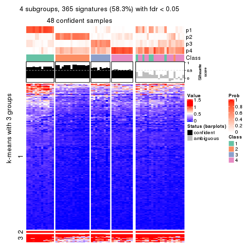
get_signatures(res, k = 5, scale_rows = FALSE)
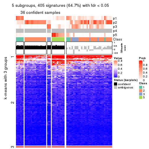
get_signatures(res, k = 6, scale_rows = FALSE)
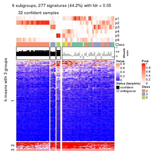
Compare the overlap of signatures from different k:
compare_signatures(res)
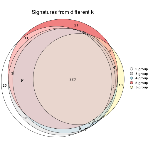
get_signature() returns a data frame invisibly. TO get the list of signatures, the function
call should be assigned to a variable explicitly. In following code, if plot argument is set
to FALSE, no heatmap is plotted while only the differential analysis is performed.
# code only for demonstration
tb = get_signature(res, k = ..., plot = FALSE)
An example of the output of tb is:
#>   which_row         fdr    mean_1    mean_2 scaled_mean_1 scaled_mean_2 km
#> 1        38 0.042760348  8.373488  9.131774    -0.5533452     0.5164555  1
#> 2        40 0.018707592  7.106213  8.469186    -0.6173731     0.5762149  1
#> 3        55 0.019134737 10.221463 11.207825    -0.6159697     0.5749050  1
#> 4        59 0.006059896  5.921854  7.869574    -0.6899429     0.6439467  1
#> 5        60 0.018055526  8.928898 10.211722    -0.6204761     0.5791110  1
#> 6        98 0.009384629 15.714769 14.887706     0.6635654    -0.6193277  2
...
The columns in tb are:
which_row: row indices corresponding to the input matrix.fdr: FDR for the differential test. mean_x: The mean value in group x.scaled_mean_x: The mean value in group x after rows are scaled.km: Row groups if k-means clustering is applied to rows.UMAP plot which shows how samples are separated.
dimension_reduction(res, k = 2, method = "UMAP")

dimension_reduction(res, k = 3, method = "UMAP")
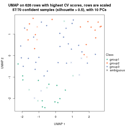
dimension_reduction(res, k = 4, method = "UMAP")
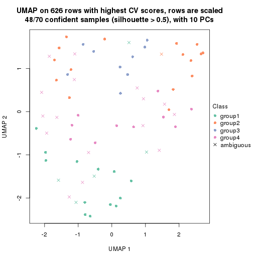
dimension_reduction(res, k = 5, method = "UMAP")
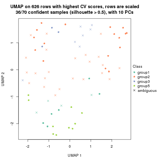
dimension_reduction(res, k = 6, method = "UMAP")
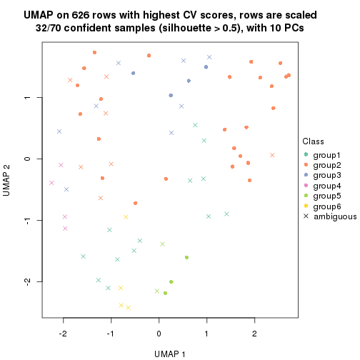
Following heatmap shows how subgroups are split when increasing k:
collect_classes(res)
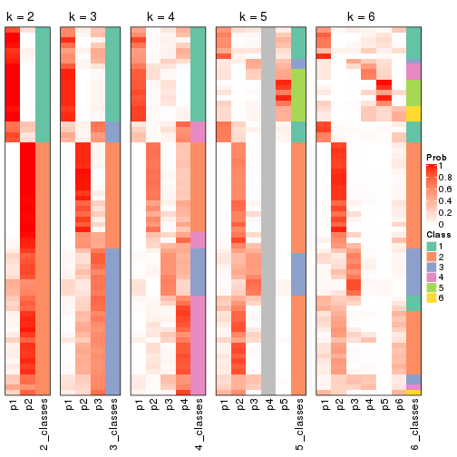
If matrix rows can be associated to genes, consider to use functional_enrichment(res,
...) to perform function enrichment for the signature genes. See this vignette for more detailed explanations.
The object with results only for a single top-value method and a single partition method can be extracted as:
res = res_list["CV", "NMF"]
# you can also extract it by
# res = res_list["CV:NMF"]
A summary of res and all the functions that can be applied to it:
res
#> A 'ConsensusPartition' object with k = 2, 3, 4, 5, 6.
#>   On a matrix with 626 rows and 70 columns.
#>   Top rows (63, 126, 188, 250, 313) are extracted by 'CV' method.
#>   Subgroups are detected by 'NMF' method.
#>   Performed in total 1250 partitions by row resampling.
#>   Best k for subgroups seems to be 2.
#>
#> Following methods can be applied to this 'ConsensusPartition' object:
#>  [1] "cola_report"             "collect_classes"         "collect_plots"
#>  [4] "collect_stats"           "colnames"                "compare_signatures"
#>  [7] "consensus_heatmap"       "dimension_reduction"     "functional_enrichment"
#> [10] "get_anno_col"            "get_anno"                "get_classes"
#> [13] "get_consensus"           "get_matrix"              "get_membership"
#> [16] "get_param"               "get_signatures"          "get_stats"
#> [19] "is_best_k"               "is_stable_k"             "membership_heatmap"
#> [22] "ncol"                    "nrow"                    "plot_ecdf"
#> [25] "rownames"                "select_partition_number" "show"
#> [28] "suggest_best_k"          "test_to_known_factors"
collect_plots() function collects all the plots made from res for all k (number of partitions)
into one single page to provide an easy and fast comparison between different k.
collect_plots(res)
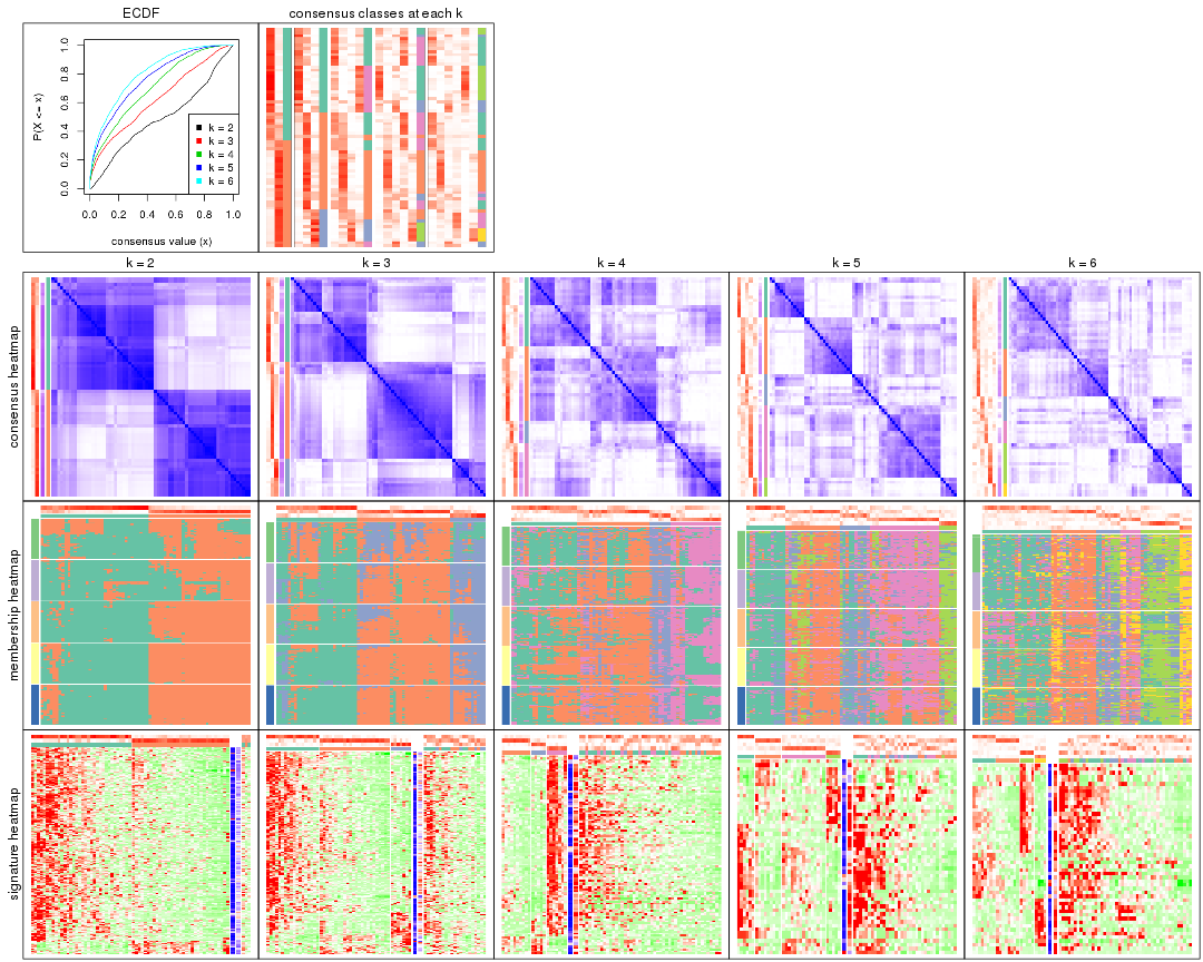
The plots are:
k and the heatmap of
predicted classes for each k.k.k.k.All the plots in panels can be made by individual functions and they are plotted later in this section.
select_partition_number() produces several plots showing different
statistics for choosing “optimized” k. There are following statistics:
k;k, the area increased is defined as \(A_k - A_{k-1}\).The detailed explanations of these statistics can be found in the cola vignette.
Generally speaking, lower PAC score, higher mean silhouette score or higher
concordance corresponds to better partition. Rand index and Jaccard index
measure how similar the current partition is compared to partition with k-1.
If they are too similar, we won't accept k is better than k-1.
select_partition_number(res)
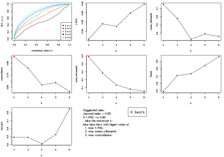
The numeric values for all these statistics can be obtained by get_stats().
get_stats(res)
#>   k 1-PAC mean_silhouette concordance area_increased  Rand Jaccard
#> 2 2 0.258           0.749       0.853         0.4930 0.493   0.493
#> 3 3 0.341           0.579       0.759         0.2839 0.708   0.492
#> 4 4 0.327           0.328       0.620         0.1321 0.733   0.412
#> 5 5 0.399           0.390       0.637         0.0794 0.845   0.527
#> 6 6 0.447           0.361       0.565         0.0497 0.965   0.848
suggest_best_k() suggests the best \(k\) based on these statistics. The rules are as follows:
suggest_best_k(res)
#> [1] 2
Following shows the table of the partitions (You need to click the show/hide
code output link to see it). The membership matrix (columns with name p*)
is inferred by
clue::cl_consensus()
function with the SE method. Basically the value in the membership matrix
represents the probability to belong to a certain group. The finall class
label for an item is determined with the group with highest probability it
belongs to.
In get_classes() function, the entropy is calculated from the membership
matrix and the silhouette score is calculated from the consensus matrix.
cbind(get_classes(res, k = 2), get_membership(res, k = 2))
#>           class entropy silhouette    p1    p2
#> SRR837437     2  0.8661    0.68616 0.288 0.712
#> SRR837438     1  0.9993   -0.00966 0.516 0.484
#> SRR837439     2  0.9286    0.58111 0.344 0.656
#> SRR837440     2  0.5408    0.81894 0.124 0.876
#> SRR837441     2  0.8861    0.64864 0.304 0.696
#> SRR837442     2  0.9896    0.29710 0.440 0.560
#> SRR837443     2  0.8555    0.68301 0.280 0.720
#> SRR837444     1  0.9286    0.50339 0.656 0.344
#> SRR837445     1  0.4298    0.82327 0.912 0.088
#> SRR837446     2  0.5737    0.81485 0.136 0.864
#> SRR837447     1  0.5408    0.81759 0.876 0.124
#> SRR837448     1  0.2043    0.81678 0.968 0.032
#> SRR837449     1  0.5946    0.77672 0.856 0.144
#> SRR837450     1  0.5519    0.75739 0.872 0.128
#> SRR837451     2  0.5408    0.81637 0.124 0.876
#> SRR837452     1  0.8661    0.61039 0.712 0.288
#> SRR837453     2  0.5737    0.84085 0.136 0.864
#> SRR837454     2  0.6887    0.78211 0.184 0.816
#> SRR837455     1  0.5842    0.81219 0.860 0.140
#> SRR837456     1  0.5178    0.81845 0.884 0.116
#> SRR837457     2  0.2948    0.84193 0.052 0.948
#> SRR837458     1  0.0938    0.83314 0.988 0.012
#> SRR837459     2  0.2423    0.84048 0.040 0.960
#> SRR837460     2  0.3879    0.83632 0.076 0.924
#> SRR837461     2  0.3431    0.83890 0.064 0.936
#> SRR837462     2  0.2603    0.83989 0.044 0.956
#> SRR837463     2  0.5408    0.81701 0.124 0.876
#> SRR837464     2  0.2603    0.83989 0.044 0.956
#> SRR837465     2  0.7056    0.76826 0.192 0.808
#> SRR837466     1  0.0000    0.83054 1.000 0.000
#> SRR837467     2  0.7453    0.74026 0.212 0.788
#> SRR837468     2  0.3114    0.82755 0.056 0.944
#> SRR837469     2  0.2603    0.84208 0.044 0.956
#> SRR837470     1  0.9491    0.56940 0.632 0.368
#> SRR837471     1  0.0376    0.83175 0.996 0.004
#> SRR837472     1  0.0376    0.83153 0.996 0.004
#> SRR837473     1  0.0376    0.82968 0.996 0.004
#> SRR837474     1  0.5059    0.81860 0.888 0.112
#> SRR837475     1  0.0000    0.83054 1.000 0.000
#> SRR837476     1  0.6623    0.79472 0.828 0.172
#> SRR837477     1  0.3274    0.80611 0.940 0.060
#> SRR837478     1  0.6148    0.73851 0.848 0.152
#> SRR837479     2  0.8081    0.72839 0.248 0.752
#> SRR837480     1  0.5294    0.78051 0.880 0.120
#> SRR837481     2  0.6438    0.82565 0.164 0.836
#> SRR837482     2  0.3733    0.84513 0.072 0.928
#> SRR837483     1  0.3274    0.80784 0.940 0.060
#> SRR837484     2  0.3584    0.82786 0.068 0.932
#> SRR837485     2  0.4690    0.81357 0.100 0.900
#> SRR837486     2  0.4562    0.81777 0.096 0.904
#> SRR837487     2  0.4431    0.82000 0.092 0.908
#> SRR837488     2  0.4562    0.82403 0.096 0.904
#> SRR837489     1  0.8386    0.68708 0.732 0.268
#> SRR837490     1  1.0000   -0.04723 0.500 0.500
#> SRR837491     1  0.9393    0.51308 0.644 0.356
#> SRR837492     1  0.1633    0.82136 0.976 0.024
#> SRR837493     1  0.9044    0.60366 0.680 0.320
#> SRR837494     2  0.7056    0.77557 0.192 0.808
#> SRR837495     1  0.3879    0.82596 0.924 0.076
#> SRR837496     1  0.3274    0.83351 0.940 0.060
#> SRR837497     1  0.1843    0.82988 0.972 0.028
#> SRR837498     1  0.9522    0.52002 0.628 0.372
#> SRR837499     1  0.4431    0.82239 0.908 0.092
#> SRR837500     1  0.4562    0.82087 0.904 0.096
#> SRR837501     2  0.4815    0.81396 0.104 0.896
#> SRR837502     1  0.4298    0.82640 0.912 0.088
#> SRR837503     1  0.1184    0.83151 0.984 0.016
#> SRR837504     2  0.5178    0.81057 0.116 0.884
#> SRR837505     2  0.4690    0.81427 0.100 0.900
#> SRR837506     2  0.4815    0.81396 0.104 0.896
cbind(get_classes(res, k = 3), get_membership(res, k = 3))
#>           class entropy silhouette    p1    p2    p3
#> SRR837437     2   0.383      0.729 0.100 0.880 0.020
#> SRR837438     2   0.520      0.627 0.220 0.772 0.008
#> SRR837439     2   0.303      0.727 0.092 0.904 0.004
#> SRR837440     2   0.807      0.208 0.080 0.576 0.344
#> SRR837441     2   0.319      0.727 0.100 0.896 0.004
#> SRR837442     2   0.375      0.709 0.144 0.856 0.000
#> SRR837443     2   0.406      0.729 0.076 0.880 0.044
#> SRR837444     2   0.581      0.495 0.304 0.692 0.004
#> SRR837445     1   0.652      0.216 0.516 0.480 0.004
#> SRR837446     2   0.785      0.330 0.076 0.608 0.316
#> SRR837447     1   0.667      0.383 0.524 0.468 0.008
#> SRR837448     1   0.312      0.675 0.892 0.000 0.108
#> SRR837449     1   0.845      0.597 0.616 0.220 0.164
#> SRR837450     1   0.565      0.492 0.688 0.000 0.312
#> SRR837451     2   0.335      0.705 0.004 0.888 0.108
#> SRR837452     2   0.956      0.189 0.308 0.472 0.220
#> SRR837453     2   0.592      0.532 0.016 0.724 0.260
#> SRR837454     2   0.232      0.737 0.028 0.944 0.028
#> SRR837455     1   0.688      0.471 0.556 0.428 0.016
#> SRR837456     1   0.623      0.558 0.624 0.372 0.004
#> SRR837457     2   0.581      0.470 0.004 0.692 0.304
#> SRR837458     1   0.269      0.711 0.932 0.036 0.032
#> SRR837459     2   0.518      0.538 0.000 0.744 0.256
#> SRR837460     2   0.394      0.669 0.000 0.844 0.156
#> SRR837461     2   0.378      0.689 0.004 0.864 0.132
#> SRR837462     2   0.473      0.641 0.004 0.800 0.196
#> SRR837463     2   0.129      0.731 0.000 0.968 0.032
#> SRR837464     2   0.445      0.633 0.000 0.808 0.192
#> SRR837465     2   0.195      0.731 0.008 0.952 0.040
#> SRR837466     1   0.216      0.694 0.936 0.000 0.064
#> SRR837467     2   0.304      0.716 0.008 0.908 0.084
#> SRR837468     3   0.627      0.310 0.000 0.456 0.544
#> SRR837469     2   0.489      0.582 0.000 0.772 0.228
#> SRR837470     1   0.920      0.236 0.476 0.368 0.156
#> SRR837471     1   0.321      0.713 0.904 0.084 0.012
#> SRR837472     1   0.347      0.711 0.904 0.040 0.056
#> SRR837473     1   0.188      0.702 0.952 0.004 0.044
#> SRR837474     1   0.590      0.578 0.648 0.352 0.000
#> SRR837475     1   0.244      0.713 0.940 0.028 0.032
#> SRR837476     2   0.679      0.266 0.324 0.648 0.028
#> SRR837477     1   0.288      0.681 0.904 0.000 0.096
#> SRR837478     1   0.622      0.244 0.568 0.000 0.432
#> SRR837479     3   0.667      0.411 0.264 0.040 0.696
#> SRR837480     1   0.627      0.397 0.644 0.008 0.348
#> SRR837481     3   0.840      0.538 0.104 0.328 0.568
#> SRR837482     2   0.650      0.351 0.020 0.664 0.316
#> SRR837483     1   0.546      0.526 0.712 0.000 0.288
#> SRR837484     3   0.614      0.606 0.012 0.304 0.684
#> SRR837485     3   0.164      0.674 0.020 0.016 0.964
#> SRR837486     3   0.408      0.676 0.048 0.072 0.880
#> SRR837487     3   0.680      0.446 0.016 0.400 0.584
#> SRR837488     3   0.740      0.464 0.036 0.412 0.552
#> SRR837489     2   0.375      0.698 0.144 0.856 0.000
#> SRR837490     2   0.341      0.716 0.124 0.876 0.000
#> SRR837491     2   0.355      0.709 0.132 0.868 0.000
#> SRR837492     1   0.271      0.687 0.912 0.000 0.088
#> SRR837493     2   0.528      0.704 0.128 0.820 0.052
#> SRR837494     2   0.337      0.737 0.040 0.908 0.052
#> SRR837495     1   0.483      0.672 0.792 0.204 0.004
#> SRR837496     1   0.295      0.710 0.920 0.060 0.020
#> SRR837497     1   0.554      0.687 0.808 0.060 0.132
#> SRR837498     2   0.399      0.684 0.124 0.864 0.012
#> SRR837499     1   0.579      0.562 0.668 0.332 0.000
#> SRR837500     1   0.608      0.490 0.612 0.388 0.000
#> SRR837501     3   0.134      0.678 0.012 0.016 0.972
#> SRR837502     1   0.642      0.377 0.572 0.424 0.004
#> SRR837503     1   0.238      0.711 0.940 0.044 0.016
#> SRR837504     3   0.713      0.429 0.028 0.392 0.580
#> SRR837505     3   0.433      0.685 0.012 0.144 0.844
#> SRR837506     3   0.134      0.676 0.016 0.012 0.972
cbind(get_classes(res, k = 4), get_membership(res, k = 4))
#>           class entropy silhouette    p1    p2    p3    p4
#> SRR837437     2   0.585     0.1593 0.428 0.544 0.020 0.008
#> SRR837438     1   0.575     0.3264 0.628 0.336 0.008 0.028
#> SRR837439     1   0.570    -0.0423 0.496 0.484 0.008 0.012
#> SRR837440     2   0.806     0.3699 0.264 0.536 0.152 0.048
#> SRR837441     1   0.558    -0.0495 0.496 0.488 0.012 0.004
#> SRR837442     1   0.585     0.0568 0.512 0.460 0.004 0.024
#> SRR837443     2   0.634     0.1657 0.420 0.532 0.024 0.024
#> SRR837444     1   0.702     0.2427 0.568 0.316 0.012 0.104
#> SRR837445     1   0.514     0.4558 0.744 0.192 0.000 0.064
#> SRR837446     2   0.888     0.2031 0.344 0.424 0.120 0.112
#> SRR837447     1   0.556     0.4903 0.724 0.196 0.004 0.076
#> SRR837448     4   0.382     0.5883 0.120 0.000 0.040 0.840
#> SRR837449     1   0.817     0.1100 0.572 0.092 0.136 0.200
#> SRR837450     4   0.507     0.5193 0.088 0.000 0.148 0.764
#> SRR837451     2   0.372     0.5810 0.096 0.852 0.052 0.000
#> SRR837452     2   0.913     0.1855 0.212 0.472 0.164 0.152
#> SRR837453     2   0.672     0.5096 0.088 0.644 0.244 0.024
#> SRR837454     2   0.623    -0.0303 0.460 0.496 0.036 0.008
#> SRR837455     1   0.665     0.3274 0.620 0.224 0.000 0.156
#> SRR837456     1   0.682     0.1709 0.612 0.148 0.004 0.236
#> SRR837457     2   0.561     0.1907 0.028 0.592 0.380 0.000
#> SRR837458     4   0.543     0.5066 0.392 0.004 0.012 0.592
#> SRR837459     2   0.438     0.4860 0.032 0.788 0.180 0.000
#> SRR837460     2   0.281     0.5910 0.080 0.896 0.024 0.000
#> SRR837461     2   0.361     0.5711 0.140 0.840 0.020 0.000
#> SRR837462     2   0.406     0.5927 0.060 0.832 0.108 0.000
#> SRR837463     2   0.326     0.5413 0.152 0.844 0.004 0.000
#> SRR837464     2   0.248     0.5972 0.032 0.916 0.052 0.000
#> SRR837465     2   0.321     0.5402 0.148 0.848 0.000 0.004
#> SRR837466     4   0.389     0.6068 0.184 0.000 0.012 0.804
#> SRR837467     2   0.309     0.5581 0.128 0.864 0.008 0.000
#> SRR837468     2   0.542     0.0188 0.000 0.572 0.412 0.016
#> SRR837469     2   0.392     0.5667 0.040 0.864 0.036 0.060
#> SRR837470     4   0.797     0.0333 0.092 0.356 0.060 0.492
#> SRR837471     4   0.557     0.3987 0.476 0.004 0.012 0.508
#> SRR837472     4   0.597     0.4528 0.420 0.004 0.032 0.544
#> SRR837473     4   0.508     0.5144 0.376 0.000 0.008 0.616
#> SRR837474     1   0.628     0.2348 0.660 0.104 0.004 0.232
#> SRR837475     4   0.523     0.4658 0.428 0.000 0.008 0.564
#> SRR837476     1   0.582     0.4364 0.652 0.300 0.008 0.040
#> SRR837477     4   0.438     0.5691 0.128 0.012 0.040 0.820
#> SRR837478     4   0.574     0.3520 0.076 0.024 0.156 0.744
#> SRR837479     4   0.889    -0.0484 0.172 0.104 0.240 0.484
#> SRR837480     4   0.635     0.3501 0.164 0.008 0.148 0.680
#> SRR837481     4   0.942    -0.3565 0.108 0.324 0.220 0.348
#> SRR837482     2   0.831     0.3158 0.156 0.572 0.136 0.136
#> SRR837483     4   0.628     0.3859 0.088 0.004 0.264 0.644
#> SRR837484     2   0.758    -0.3915 0.012 0.432 0.420 0.136
#> SRR837485     3   0.551     0.6558 0.004 0.080 0.732 0.184
#> SRR837486     3   0.763     0.4997 0.000 0.228 0.460 0.312
#> SRR837487     3   0.724     0.3556 0.008 0.408 0.472 0.112
#> SRR837488     2   0.791    -0.3009 0.020 0.440 0.384 0.156
#> SRR837489     1   0.499     0.1372 0.532 0.468 0.000 0.000
#> SRR837490     1   0.520     0.2233 0.592 0.400 0.004 0.004
#> SRR837491     1   0.500     0.2821 0.604 0.392 0.000 0.004
#> SRR837492     4   0.451     0.6008 0.224 0.000 0.020 0.756
#> SRR837493     1   0.646     0.2704 0.544 0.400 0.036 0.020
#> SRR837494     2   0.558     0.4661 0.248 0.696 0.052 0.004
#> SRR837495     1   0.374     0.3630 0.824 0.016 0.000 0.160
#> SRR837496     1   0.589    -0.2721 0.528 0.016 0.012 0.444
#> SRR837497     1   0.771    -0.1745 0.504 0.012 0.180 0.304
#> SRR837498     2   0.544     0.0237 0.456 0.532 0.004 0.008
#> SRR837499     1   0.267     0.4782 0.908 0.040 0.000 0.052
#> SRR837500     1   0.435     0.4769 0.816 0.080 0.000 0.104
#> SRR837501     3   0.358     0.6826 0.008 0.060 0.872 0.060
#> SRR837502     1   0.519     0.5169 0.780 0.128 0.016 0.076
#> SRR837503     4   0.541     0.3784 0.492 0.000 0.012 0.496
#> SRR837504     3   0.524     0.5544 0.012 0.260 0.708 0.020
#> SRR837505     3   0.390     0.6890 0.000 0.164 0.816 0.020
#> SRR837506     3   0.438     0.6512 0.020 0.068 0.836 0.076
cbind(get_classes(res, k = 5), get_membership(res, k = 5))
#>           class entropy silhouette    p1    p2    p3    p4    p5
#> SRR837437     4   0.595     0.2706 0.012 0.356 0.056 0.564 0.012
#> SRR837438     4   0.426     0.6365 0.064 0.080 0.036 0.816 0.004
#> SRR837439     4   0.560     0.5081 0.012 0.216 0.080 0.680 0.012
#> SRR837440     2   0.828     0.1226 0.008 0.352 0.188 0.340 0.112
#> SRR837441     4   0.465     0.4989 0.004 0.248 0.028 0.712 0.008
#> SRR837442     4   0.714     0.4078 0.088 0.268 0.088 0.548 0.008
#> SRR837443     4   0.610     0.2725 0.000 0.324 0.116 0.552 0.008
#> SRR837444     4   0.441     0.5657 0.008 0.052 0.180 0.760 0.000
#> SRR837445     4   0.391     0.6196 0.024 0.064 0.084 0.828 0.000
#> SRR837446     3   0.678    -0.0771 0.000 0.176 0.412 0.400 0.012
#> SRR837447     4   0.709     0.5104 0.148 0.176 0.072 0.592 0.012
#> SRR837448     1   0.458     0.2904 0.608 0.004 0.380 0.004 0.004
#> SRR837449     4   0.830     0.2500 0.272 0.112 0.036 0.456 0.124
#> SRR837450     1   0.539     0.1924 0.544 0.008 0.412 0.004 0.032
#> SRR837451     2   0.526     0.5966 0.008 0.740 0.044 0.152 0.056
#> SRR837452     2   0.928     0.2125 0.188 0.392 0.156 0.172 0.092
#> SRR837453     2   0.730     0.2975 0.004 0.480 0.056 0.140 0.320
#> SRR837454     4   0.621     0.5232 0.008 0.232 0.068 0.640 0.052
#> SRR837455     4   0.760     0.0998 0.348 0.248 0.036 0.364 0.004
#> SRR837456     1   0.718     0.1177 0.492 0.140 0.040 0.320 0.008
#> SRR837457     2   0.590     0.0862 0.004 0.500 0.024 0.040 0.432
#> SRR837458     1   0.315     0.6186 0.880 0.032 0.028 0.056 0.004
#> SRR837459     2   0.464     0.4718 0.000 0.728 0.012 0.040 0.220
#> SRR837460     2   0.337     0.6222 0.000 0.836 0.000 0.120 0.044
#> SRR837461     2   0.440     0.5895 0.000 0.768 0.032 0.176 0.024
#> SRR837462     2   0.437     0.6162 0.004 0.788 0.008 0.124 0.076
#> SRR837463     2   0.405     0.5941 0.008 0.788 0.016 0.176 0.012
#> SRR837464     2   0.304     0.6135 0.000 0.872 0.020 0.088 0.020
#> SRR837465     2   0.492     0.5242 0.008 0.712 0.052 0.224 0.004
#> SRR837466     1   0.422     0.4486 0.704 0.000 0.280 0.012 0.004
#> SRR837467     2   0.490     0.5289 0.012 0.728 0.032 0.212 0.016
#> SRR837468     2   0.564     0.2991 0.004 0.636 0.056 0.020 0.284
#> SRR837469     2   0.487     0.5420 0.012 0.756 0.156 0.064 0.012
#> SRR837470     3   0.725     0.2795 0.152 0.324 0.480 0.032 0.012
#> SRR837471     1   0.332     0.6159 0.832 0.000 0.032 0.136 0.000
#> SRR837472     1   0.291     0.6302 0.880 0.004 0.016 0.088 0.012
#> SRR837473     1   0.214     0.6298 0.916 0.000 0.016 0.064 0.004
#> SRR837474     1   0.661    -0.0639 0.452 0.068 0.044 0.432 0.004
#> SRR837475     1   0.301     0.6253 0.868 0.008 0.016 0.104 0.004
#> SRR837476     4   0.632     0.5704 0.176 0.104 0.056 0.656 0.008
#> SRR837477     3   0.455    -0.1474 0.472 0.000 0.520 0.008 0.000
#> SRR837478     3   0.402     0.2511 0.272 0.000 0.716 0.012 0.000
#> SRR837479     3   0.484     0.4077 0.040 0.068 0.796 0.064 0.032
#> SRR837480     3   0.630     0.2639 0.248 0.008 0.620 0.088 0.036
#> SRR837481     3   0.656     0.2370 0.016 0.232 0.612 0.032 0.108
#> SRR837482     3   0.708    -0.0485 0.000 0.404 0.432 0.080 0.084
#> SRR837483     1   0.496     0.4394 0.736 0.016 0.088 0.000 0.160
#> SRR837484     2   0.722    -0.2300 0.020 0.416 0.212 0.004 0.348
#> SRR837485     5   0.593     0.5553 0.052 0.088 0.192 0.000 0.668
#> SRR837486     3   0.772    -0.2735 0.056 0.252 0.348 0.000 0.344
#> SRR837487     5   0.752     0.3244 0.064 0.336 0.124 0.012 0.464
#> SRR837488     2   0.786    -0.1654 0.028 0.408 0.228 0.028 0.308
#> SRR837489     4   0.439     0.5407 0.008 0.264 0.012 0.712 0.004
#> SRR837490     4   0.336     0.6153 0.008 0.132 0.016 0.840 0.004
#> SRR837491     4   0.375     0.6044 0.008 0.180 0.012 0.796 0.004
#> SRR837492     1   0.362     0.5296 0.788 0.004 0.196 0.012 0.000
#> SRR837493     4   0.518     0.5955 0.032 0.132 0.032 0.760 0.044
#> SRR837494     2   0.664     0.2095 0.008 0.500 0.052 0.384 0.056
#> SRR837495     4   0.483     0.5011 0.200 0.000 0.088 0.712 0.000
#> SRR837496     3   0.680     0.0536 0.264 0.004 0.440 0.292 0.000
#> SRR837497     4   0.891     0.1181 0.196 0.040 0.172 0.400 0.192
#> SRR837498     4   0.607     0.3999 0.020 0.284 0.088 0.604 0.004
#> SRR837499     4   0.340     0.5707 0.172 0.004 0.012 0.812 0.000
#> SRR837500     4   0.400     0.5496 0.204 0.008 0.020 0.768 0.000
#> SRR837501     5   0.420     0.6629 0.036 0.068 0.072 0.004 0.820
#> SRR837502     4   0.517     0.6272 0.100 0.072 0.036 0.768 0.024
#> SRR837503     1   0.598     0.4240 0.584 0.000 0.176 0.240 0.000
#> SRR837504     5   0.491     0.6547 0.024 0.160 0.024 0.032 0.760
#> SRR837505     5   0.352     0.6962 0.000 0.144 0.024 0.008 0.824
#> SRR837506     5   0.500     0.6067 0.016 0.076 0.132 0.016 0.760
cbind(get_classes(res, k = 6), get_membership(res, k = 6))
#>           class entropy silhouette    p1    p2    p3    p4    p5    p6
#> SRR837437     1   0.707     0.2820 0.500 0.284 0.048 0.128 0.012 0.028
#> SRR837438     1   0.599     0.5666 0.688 0.092 0.044 0.064 0.100 0.012
#> SRR837439     1   0.646     0.4946 0.624 0.196 0.060 0.064 0.032 0.024
#> SRR837440     4   0.835     0.0267 0.256 0.228 0.092 0.340 0.004 0.080
#> SRR837441     1   0.564     0.4667 0.660 0.224 0.028 0.040 0.012 0.036
#> SRR837442     1   0.834     0.2866 0.416 0.260 0.056 0.128 0.104 0.036
#> SRR837443     1   0.700     0.3299 0.520 0.236 0.100 0.120 0.000 0.024
#> SRR837444     1   0.585     0.4771 0.664 0.076 0.188 0.032 0.016 0.024
#> SRR837445     1   0.450     0.5347 0.768 0.056 0.136 0.020 0.012 0.008
#> SRR837446     3   0.746    -0.0953 0.380 0.100 0.380 0.080 0.000 0.060
#> SRR837447     1   0.784     0.4287 0.508 0.208 0.084 0.056 0.104 0.040
#> SRR837448     5   0.432     0.2323 0.000 0.000 0.400 0.012 0.580 0.008
#> SRR837449     1   0.874     0.3150 0.396 0.184 0.040 0.124 0.184 0.072
#> SRR837450     5   0.504     0.1512 0.000 0.000 0.420 0.028 0.524 0.028
#> SRR837451     2   0.555     0.5282 0.124 0.668 0.008 0.156 0.000 0.044
#> SRR837452     2   0.930     0.1295 0.144 0.352 0.116 0.176 0.140 0.072
#> SRR837453     2   0.779     0.2719 0.104 0.416 0.036 0.168 0.004 0.272
#> SRR837454     1   0.762     0.3214 0.456 0.284 0.072 0.088 0.004 0.096
#> SRR837455     1   0.847     0.1351 0.296 0.288 0.036 0.072 0.264 0.044
#> SRR837456     5   0.805     0.0223 0.264 0.180 0.056 0.036 0.420 0.044
#> SRR837457     2   0.653     0.1696 0.040 0.464 0.008 0.144 0.000 0.344
#> SRR837458     5   0.370     0.5150 0.008 0.052 0.044 0.024 0.844 0.028
#> SRR837459     2   0.542     0.4709 0.016 0.648 0.008 0.128 0.000 0.200
#> SRR837460     2   0.337     0.6089 0.056 0.844 0.000 0.048 0.000 0.052
#> SRR837461     2   0.533     0.5553 0.100 0.720 0.032 0.096 0.000 0.052
#> SRR837462     2   0.389     0.5871 0.032 0.788 0.000 0.036 0.000 0.144
#> SRR837463     2   0.375     0.5947 0.072 0.808 0.004 0.104 0.000 0.012
#> SRR837464     2   0.388     0.5781 0.036 0.804 0.004 0.116 0.000 0.040
#> SRR837465     2   0.424     0.5402 0.140 0.776 0.048 0.024 0.000 0.012
#> SRR837466     5   0.424     0.3472 0.004 0.000 0.304 0.012 0.668 0.012
#> SRR837467     2   0.397     0.5805 0.084 0.820 0.024 0.036 0.004 0.032
#> SRR837468     2   0.660     0.1983 0.004 0.488 0.040 0.168 0.004 0.296
#> SRR837469     2   0.636     0.3957 0.024 0.620 0.148 0.152 0.008 0.048
#> SRR837470     3   0.762     0.1522 0.004 0.336 0.396 0.092 0.136 0.036
#> SRR837471     5   0.501     0.5070 0.116 0.020 0.064 0.024 0.752 0.024
#> SRR837472     5   0.347     0.5407 0.084 0.000 0.068 0.008 0.832 0.008
#> SRR837473     5   0.261     0.5437 0.056 0.000 0.016 0.028 0.892 0.008
#> SRR837474     5   0.778    -0.0924 0.360 0.104 0.064 0.044 0.396 0.032
#> SRR837475     5   0.261     0.5401 0.072 0.000 0.016 0.012 0.888 0.012
#> SRR837476     1   0.685     0.4794 0.612 0.088 0.064 0.024 0.160 0.052
#> SRR837477     3   0.442    -0.0609 0.008 0.000 0.548 0.004 0.432 0.008
#> SRR837478     3   0.395     0.2950 0.004 0.000 0.724 0.032 0.240 0.000
#> SRR837479     3   0.630     0.3640 0.076 0.040 0.676 0.108 0.048 0.052
#> SRR837480     3   0.636     0.3038 0.080 0.000 0.588 0.040 0.240 0.052
#> SRR837481     3   0.621    -0.2266 0.032 0.092 0.464 0.400 0.004 0.008
#> SRR837482     4   0.711     0.3262 0.052 0.220 0.284 0.428 0.000 0.016
#> SRR837483     5   0.555     0.3417 0.000 0.004 0.084 0.196 0.656 0.060
#> SRR837484     4   0.483     0.4687 0.000 0.168 0.068 0.724 0.008 0.032
#> SRR837485     4   0.584    -0.1482 0.000 0.040 0.084 0.584 0.008 0.284
#> SRR837486     4   0.512     0.4022 0.000 0.084 0.140 0.720 0.036 0.020
#> SRR837487     4   0.621     0.2976 0.012 0.148 0.036 0.636 0.024 0.144
#> SRR837488     4   0.574     0.4749 0.032 0.208 0.060 0.660 0.008 0.032
#> SRR837489     1   0.559     0.3744 0.552 0.364 0.036 0.032 0.012 0.004
#> SRR837490     1   0.524     0.5241 0.692 0.204 0.024 0.040 0.004 0.036
#> SRR837491     1   0.618     0.5022 0.624 0.232 0.040 0.048 0.028 0.028
#> SRR837492     5   0.473     0.3797 0.000 0.000 0.256 0.052 0.672 0.020
#> SRR837493     1   0.727     0.5036 0.572 0.192 0.056 0.048 0.068 0.064
#> SRR837494     2   0.726     0.1758 0.280 0.444 0.036 0.200 0.004 0.036
#> SRR837495     1   0.488     0.4771 0.724 0.004 0.144 0.016 0.104 0.008
#> SRR837496     3   0.645     0.1807 0.288 0.004 0.488 0.012 0.196 0.012
#> SRR837497     1   0.892     0.0402 0.320 0.012 0.164 0.136 0.140 0.228
#> SRR837498     1   0.676     0.4156 0.556 0.268 0.068 0.052 0.016 0.040
#> SRR837499     1   0.386     0.5418 0.800 0.012 0.032 0.012 0.140 0.004
#> SRR837500     1   0.512     0.5364 0.732 0.056 0.028 0.016 0.148 0.020
#> SRR837501     6   0.542     0.5607 0.008 0.028 0.032 0.344 0.008 0.580
#> SRR837502     1   0.745     0.5139 0.576 0.148 0.084 0.056 0.076 0.060
#> SRR837503     5   0.649     0.2484 0.276 0.000 0.192 0.036 0.492 0.004
#> SRR837504     6   0.635     0.5828 0.032 0.092 0.024 0.280 0.008 0.564
#> SRR837505     6   0.567     0.5660 0.004 0.088 0.012 0.324 0.008 0.564
#> SRR837506     6   0.453     0.5699 0.000 0.044 0.084 0.088 0.012 0.772
Heatmaps for the consensus matrix. It visualizes the probability of two samples to be in a same group.
consensus_heatmap(res, k = 2)
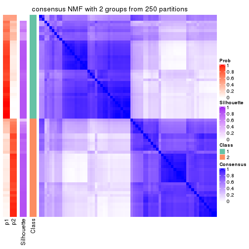
consensus_heatmap(res, k = 3)
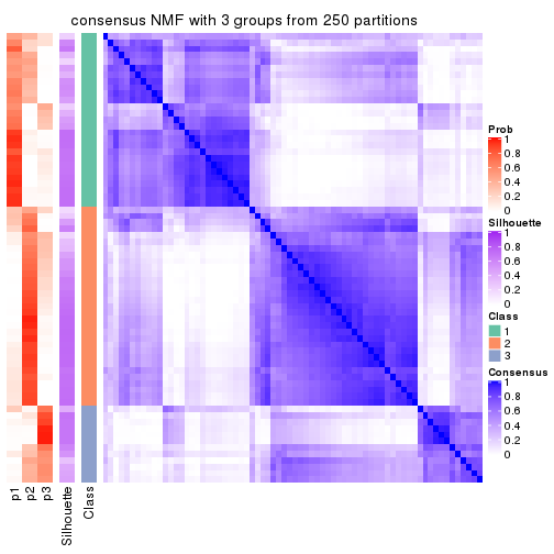
consensus_heatmap(res, k = 4)
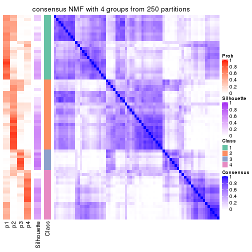
consensus_heatmap(res, k = 5)
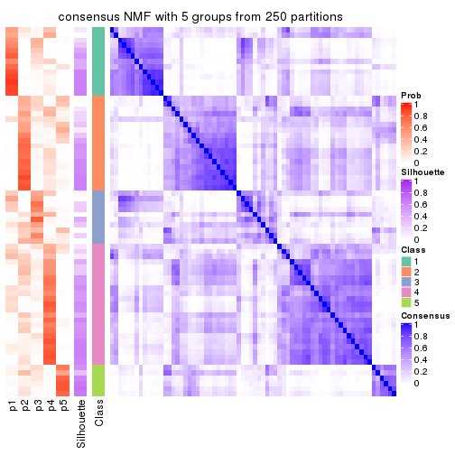
consensus_heatmap(res, k = 6)
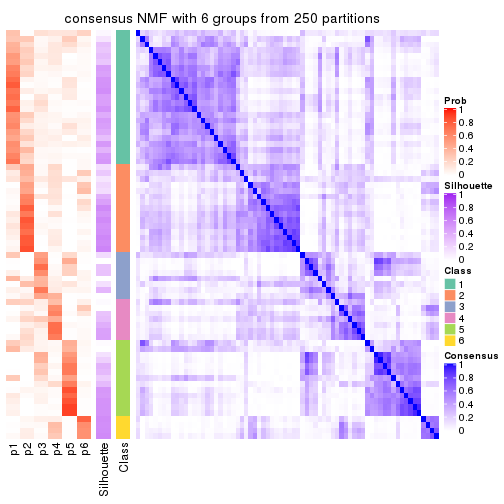
Heatmaps for the membership of samples in all partitions to see how consistent they are:
membership_heatmap(res, k = 2)
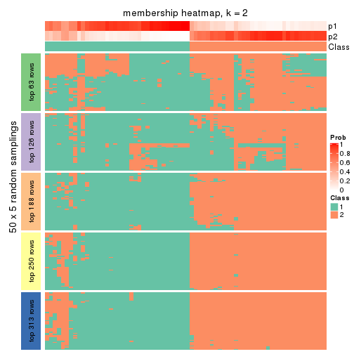
membership_heatmap(res, k = 3)
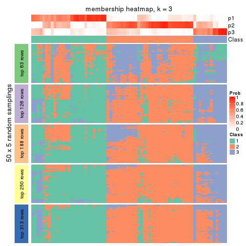
membership_heatmap(res, k = 4)
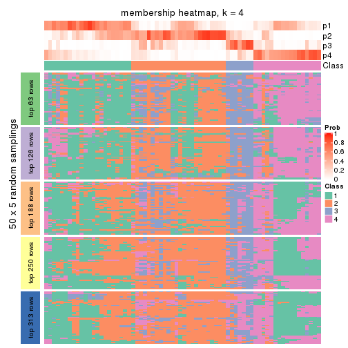
membership_heatmap(res, k = 5)
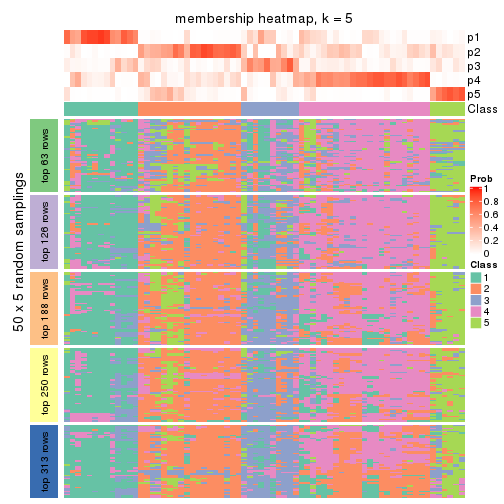
membership_heatmap(res, k = 6)
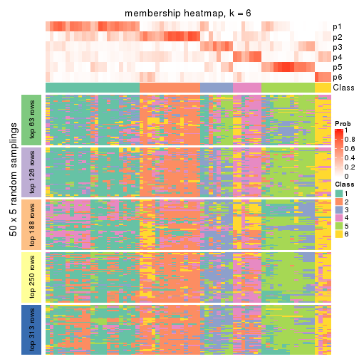
As soon as we have had the classes for columns, we can look for signatures which are significantly different between classes which can be candidate marks for certain classes. Following are the heatmaps for signatures.
Signature heatmaps where rows are scaled:
get_signatures(res, k = 2)
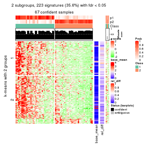
get_signatures(res, k = 3)
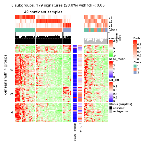
get_signatures(res, k = 4)
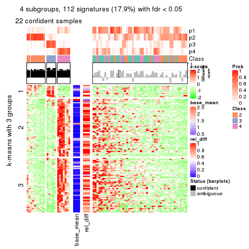
get_signatures(res, k = 5)
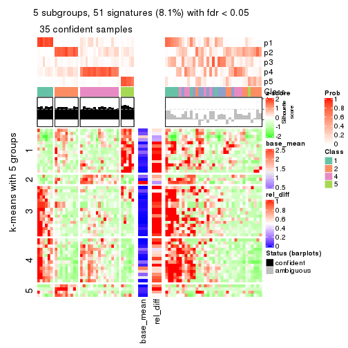
get_signatures(res, k = 6)
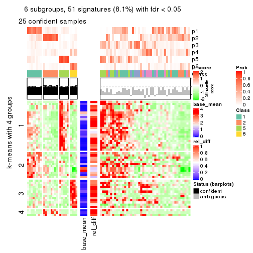
Signature heatmaps where rows are not scaled:
get_signatures(res, k = 2, scale_rows = FALSE)
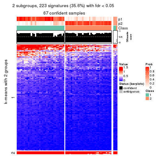
get_signatures(res, k = 3, scale_rows = FALSE)
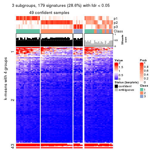
get_signatures(res, k = 4, scale_rows = FALSE)
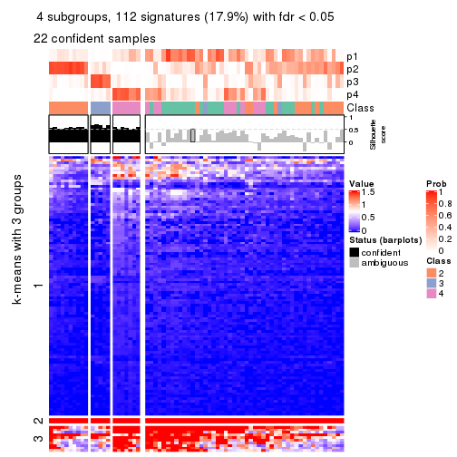
get_signatures(res, k = 5, scale_rows = FALSE)
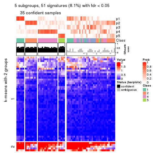
get_signatures(res, k = 6, scale_rows = FALSE)
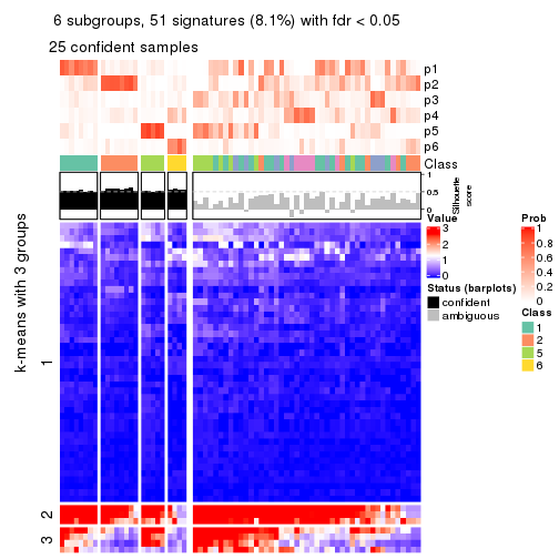
Compare the overlap of signatures from different k:
compare_signatures(res)
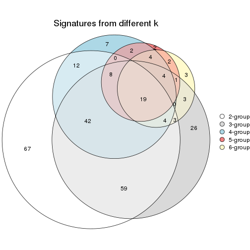
get_signature() returns a data frame invisibly. TO get the list of signatures, the function
call should be assigned to a variable explicitly. In following code, if plot argument is set
to FALSE, no heatmap is plotted while only the differential analysis is performed.
# code only for demonstration
tb = get_signature(res, k = ..., plot = FALSE)
An example of the output of tb is:
#>   which_row         fdr    mean_1    mean_2 scaled_mean_1 scaled_mean_2 km
#> 1        38 0.042760348  8.373488  9.131774    -0.5533452     0.5164555  1
#> 2        40 0.018707592  7.106213  8.469186    -0.6173731     0.5762149  1
#> 3        55 0.019134737 10.221463 11.207825    -0.6159697     0.5749050  1
#> 4        59 0.006059896  5.921854  7.869574    -0.6899429     0.6439467  1
#> 5        60 0.018055526  8.928898 10.211722    -0.6204761     0.5791110  1
#> 6        98 0.009384629 15.714769 14.887706     0.6635654    -0.6193277  2
...
The columns in tb are:
which_row: row indices corresponding to the input matrix.fdr: FDR for the differential test. mean_x: The mean value in group x.scaled_mean_x: The mean value in group x after rows are scaled.km: Row groups if k-means clustering is applied to rows.UMAP plot which shows how samples are separated.
dimension_reduction(res, k = 2, method = "UMAP")

dimension_reduction(res, k = 3, method = "UMAP")
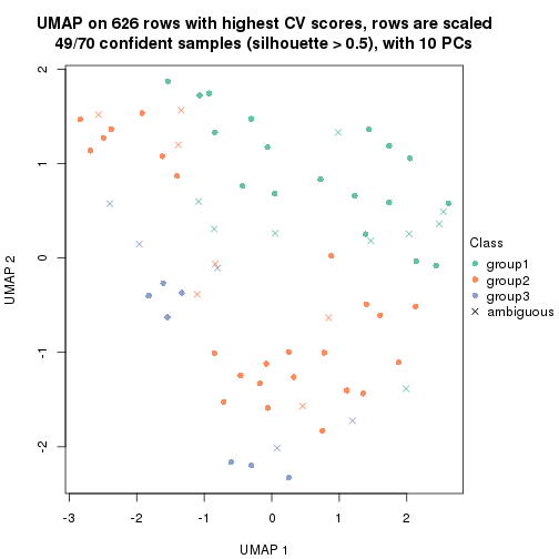
dimension_reduction(res, k = 4, method = "UMAP")
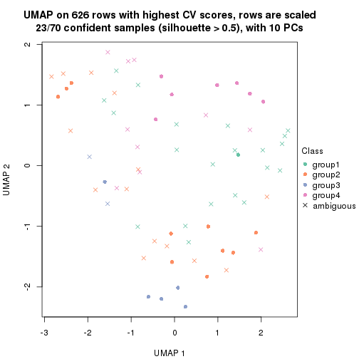
dimension_reduction(res, k = 5, method = "UMAP")
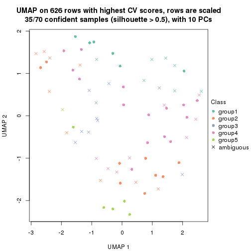
dimension_reduction(res, k = 6, method = "UMAP")
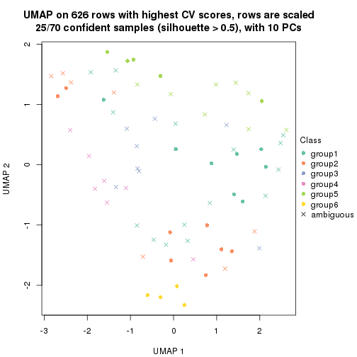
Following heatmap shows how subgroups are split when increasing k:
collect_classes(res)
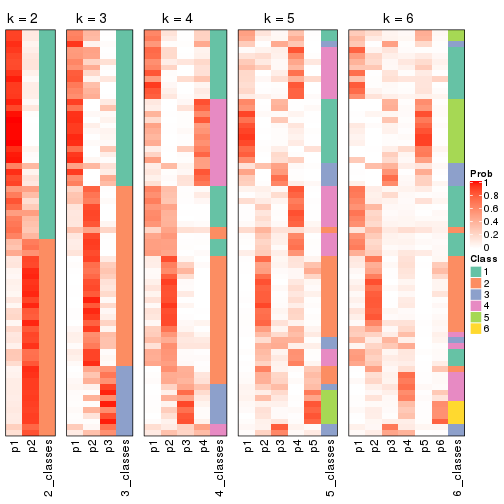
If matrix rows can be associated to genes, consider to use functional_enrichment(res,
...) to perform function enrichment for the signature genes. See this vignette for more detailed explanations.
The object with results only for a single top-value method and a single partition method can be extracted as:
res = res_list["MAD", "hclust"]
# you can also extract it by
# res = res_list["MAD:hclust"]
A summary of res and all the functions that can be applied to it:
res
#> A 'ConsensusPartition' object with k = 2, 3, 4, 5, 6.
#>   On a matrix with 626 rows and 70 columns.
#>   Top rows (63, 126, 188, 250, 313) are extracted by 'MAD' method.
#>   Subgroups are detected by 'hclust' method.
#>   Performed in total 1250 partitions by row resampling.
#>   Best k for subgroups seems to be 3.
#>
#> Following methods can be applied to this 'ConsensusPartition' object:
#>  [1] "cola_report"             "collect_classes"         "collect_plots"
#>  [4] "collect_stats"           "colnames"                "compare_signatures"
#>  [7] "consensus_heatmap"       "dimension_reduction"     "functional_enrichment"
#> [10] "get_anno_col"            "get_anno"                "get_classes"
#> [13] "get_consensus"           "get_matrix"              "get_membership"
#> [16] "get_param"               "get_signatures"          "get_stats"
#> [19] "is_best_k"               "is_stable_k"             "membership_heatmap"
#> [22] "ncol"                    "nrow"                    "plot_ecdf"
#> [25] "rownames"                "select_partition_number" "show"
#> [28] "suggest_best_k"          "test_to_known_factors"
collect_plots() function collects all the plots made from res for all k (number of partitions)
into one single page to provide an easy and fast comparison between different k.
collect_plots(res)
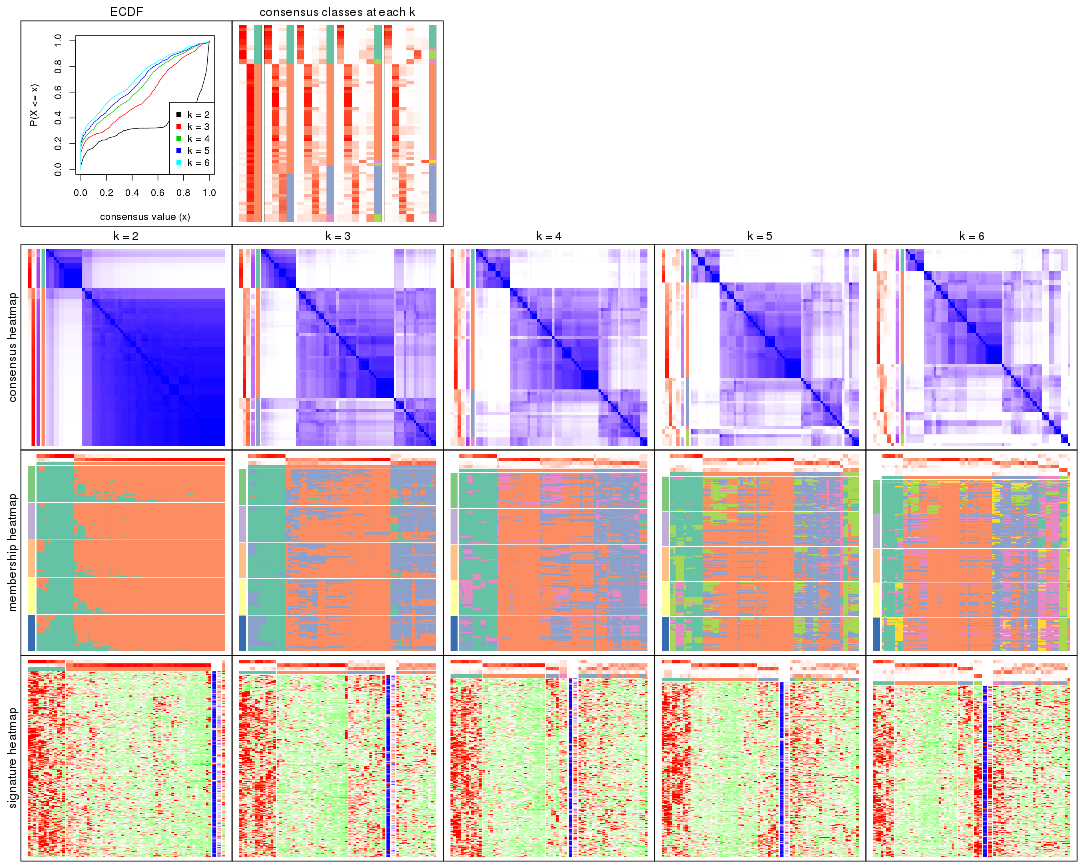
The plots are:
k and the heatmap of
predicted classes for each k.k.k.k.All the plots in panels can be made by individual functions and they are plotted later in this section.
select_partition_number() produces several plots showing different
statistics for choosing “optimized” k. There are following statistics:
k;k, the area increased is defined as \(A_k - A_{k-1}\).The detailed explanations of these statistics can be found in the cola vignette.
Generally speaking, lower PAC score, higher mean silhouette score or higher
concordance corresponds to better partition. Rand index and Jaccard index
measure how similar the current partition is compared to partition with k-1.
If they are too similar, we won't accept k is better than k-1.
select_partition_number(res)
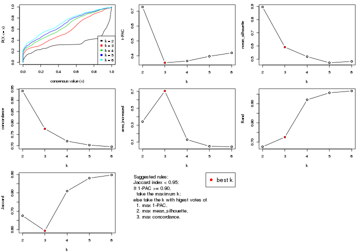
The numeric values for all these statistics can be obtained by get_stats().
get_stats(res)
#>   k 1-PAC mean_silhouette concordance area_increased  Rand Jaccard
#> 2 2 0.728           0.896       0.942         0.3421 0.675   0.675
#> 3 3 0.354           0.591       0.775         0.7050 0.725   0.594
#> 4 4 0.366           0.519       0.721         0.1280 0.920   0.810
#> 5 5 0.397           0.472       0.703         0.0496 0.957   0.881
#> 6 6 0.420           0.482       0.696         0.0438 0.966   0.898
suggest_best_k() suggests the best \(k\) based on these statistics. The rules are as follows:
suggest_best_k(res)
#> [1] 3
Following shows the table of the partitions (You need to click the show/hide
code output link to see it). The membership matrix (columns with name p*)
is inferred by
clue::cl_consensus()
function with the SE method. Basically the value in the membership matrix
represents the probability to belong to a certain group. The finall class
label for an item is determined with the group with highest probability it
belongs to.
In get_classes() function, the entropy is calculated from the membership
matrix and the silhouette score is calculated from the consensus matrix.
cbind(get_classes(res, k = 2), get_membership(res, k = 2))
#>           class entropy silhouette    p1    p2
#> SRR837437     2  0.0376      0.945 0.004 0.996
#> SRR837438     2  0.5629      0.870 0.132 0.868
#> SRR837439     2  0.0938      0.946 0.012 0.988
#> SRR837440     2  0.0672      0.946 0.008 0.992
#> SRR837441     2  0.0376      0.945 0.004 0.996
#> SRR837442     2  0.0000      0.944 0.000 1.000
#> SRR837443     2  0.1414      0.946 0.020 0.980
#> SRR837444     2  0.3274      0.927 0.060 0.940
#> SRR837445     2  0.4431      0.908 0.092 0.908
#> SRR837446     2  0.1184      0.946 0.016 0.984
#> SRR837447     1  0.0000      0.910 1.000 0.000
#> SRR837448     1  0.0000      0.910 1.000 0.000
#> SRR837449     1  0.5294      0.857 0.880 0.120
#> SRR837450     1  0.0000      0.910 1.000 0.000
#> SRR837451     2  0.0000      0.944 0.000 1.000
#> SRR837452     2  0.0376      0.945 0.004 0.996
#> SRR837453     2  0.0000      0.944 0.000 1.000
#> SRR837454     2  0.0000      0.944 0.000 1.000
#> SRR837455     1  0.0000      0.910 1.000 0.000
#> SRR837456     1  0.0000      0.910 1.000 0.000
#> SRR837457     2  0.0000      0.944 0.000 1.000
#> SRR837458     1  0.0000      0.910 1.000 0.000
#> SRR837459     2  0.0000      0.944 0.000 1.000
#> SRR837460     2  0.0000      0.944 0.000 1.000
#> SRR837461     2  0.0376      0.946 0.004 0.996
#> SRR837462     2  0.4815      0.897 0.104 0.896
#> SRR837463     2  0.2603      0.938 0.044 0.956
#> SRR837464     2  0.2423      0.939 0.040 0.960
#> SRR837465     2  0.5629      0.870 0.132 0.868
#> SRR837466     1  0.0000      0.910 1.000 0.000
#> SRR837467     2  0.0000      0.944 0.000 1.000
#> SRR837468     2  0.2778      0.936 0.048 0.952
#> SRR837469     1  0.1843      0.907 0.972 0.028
#> SRR837470     1  0.1843      0.907 0.972 0.028
#> SRR837471     2  0.0938      0.946 0.012 0.988
#> SRR837472     2  0.0938      0.946 0.012 0.988
#> SRR837473     2  0.4690      0.899 0.100 0.900
#> SRR837474     2  0.0938      0.946 0.012 0.988
#> SRR837475     2  0.0672      0.946 0.008 0.992
#> SRR837476     2  0.0376      0.945 0.004 0.996
#> SRR837477     2  0.3431      0.927 0.064 0.936
#> SRR837478     2  0.1184      0.945 0.016 0.984
#> SRR837479     2  0.1843      0.944 0.028 0.972
#> SRR837480     2  0.1184      0.945 0.016 0.984
#> SRR837481     2  0.2236      0.941 0.036 0.964
#> SRR837482     2  0.2778      0.936 0.048 0.952
#> SRR837483     2  0.9393      0.488 0.356 0.644
#> SRR837484     2  0.1184      0.946 0.016 0.984
#> SRR837485     2  0.1633      0.944 0.024 0.976
#> SRR837486     2  0.4562      0.907 0.096 0.904
#> SRR837487     2  0.0376      0.945 0.004 0.996
#> SRR837488     2  0.0000      0.944 0.000 1.000
#> SRR837489     2  0.1414      0.945 0.020 0.980
#> SRR837490     2  0.1414      0.945 0.020 0.980
#> SRR837491     2  0.2948      0.933 0.052 0.948
#> SRR837492     2  0.4690      0.899 0.100 0.900
#> SRR837493     2  0.6343      0.838 0.160 0.840
#> SRR837494     2  0.0000      0.944 0.000 1.000
#> SRR837495     2  0.4161      0.914 0.084 0.916
#> SRR837496     1  0.8386      0.671 0.732 0.268
#> SRR837497     1  0.7299      0.768 0.796 0.204
#> SRR837498     1  0.4939      0.866 0.892 0.108
#> SRR837499     2  0.9170      0.549 0.332 0.668
#> SRR837500     2  0.9170      0.549 0.332 0.668
#> SRR837501     2  0.1414      0.945 0.020 0.980
#> SRR837502     2  0.9044      0.574 0.320 0.680
#> SRR837503     1  0.8608      0.641 0.716 0.284
#> SRR837504     2  0.0672      0.946 0.008 0.992
#> SRR837505     2  0.0376      0.945 0.004 0.996
#> SRR837506     2  0.0376      0.945 0.004 0.996
cbind(get_classes(res, k = 3), get_membership(res, k = 3))
#>           class entropy silhouette    p1    p2    p3
#> SRR837437     2  0.3619     0.6966 0.000 0.864 0.136
#> SRR837438     3  0.5850     0.6913 0.040 0.188 0.772
#> SRR837439     2  0.4974     0.6475 0.000 0.764 0.236
#> SRR837440     2  0.4974     0.6427 0.000 0.764 0.236
#> SRR837441     2  0.4605     0.6644 0.000 0.796 0.204
#> SRR837442     2  0.1753     0.7072 0.000 0.952 0.048
#> SRR837443     2  0.5560     0.5897 0.000 0.700 0.300
#> SRR837444     3  0.6379     0.4525 0.008 0.368 0.624
#> SRR837445     2  0.7138     0.1794 0.024 0.540 0.436
#> SRR837446     2  0.6126     0.3526 0.000 0.600 0.400
#> SRR837447     1  0.0592     0.8739 0.988 0.000 0.012
#> SRR837448     1  0.1643     0.8657 0.956 0.000 0.044
#> SRR837449     1  0.4521     0.8152 0.816 0.004 0.180
#> SRR837450     1  0.1643     0.8657 0.956 0.000 0.044
#> SRR837451     2  0.0237     0.6898 0.000 0.996 0.004
#> SRR837452     2  0.2711     0.6886 0.000 0.912 0.088
#> SRR837453     2  0.0237     0.6898 0.000 0.996 0.004
#> SRR837454     2  0.0237     0.6898 0.000 0.996 0.004
#> SRR837455     1  0.0592     0.8739 0.988 0.000 0.012
#> SRR837456     1  0.0592     0.8739 0.988 0.000 0.012
#> SRR837457     2  0.0237     0.6898 0.000 0.996 0.004
#> SRR837458     1  0.1411     0.8694 0.964 0.000 0.036
#> SRR837459     2  0.0237     0.6898 0.000 0.996 0.004
#> SRR837460     2  0.0237     0.6898 0.000 0.996 0.004
#> SRR837461     2  0.5785     0.4944 0.000 0.668 0.332
#> SRR837462     3  0.6703     0.6958 0.052 0.236 0.712
#> SRR837463     3  0.5953     0.6542 0.012 0.280 0.708
#> SRR837464     3  0.5864     0.6434 0.008 0.288 0.704
#> SRR837465     3  0.6319     0.6692 0.040 0.228 0.732
#> SRR837466     1  0.1643     0.8657 0.956 0.000 0.044
#> SRR837467     2  0.3116     0.7070 0.000 0.892 0.108
#> SRR837468     3  0.5378     0.6490 0.008 0.236 0.756
#> SRR837469     1  0.2066     0.8702 0.940 0.000 0.060
#> SRR837470     1  0.2066     0.8702 0.940 0.000 0.060
#> SRR837471     2  0.2711     0.7081 0.000 0.912 0.088
#> SRR837472     2  0.2711     0.7081 0.000 0.912 0.088
#> SRR837473     2  0.7187     0.0111 0.024 0.496 0.480
#> SRR837474     2  0.2625     0.7086 0.000 0.916 0.084
#> SRR837475     2  0.2537     0.7093 0.000 0.920 0.080
#> SRR837476     2  0.2066     0.7092 0.000 0.940 0.060
#> SRR837477     2  0.6823     0.5262 0.036 0.668 0.296
#> SRR837478     2  0.5363     0.5832 0.000 0.724 0.276
#> SRR837479     3  0.6309    -0.0387 0.000 0.496 0.504
#> SRR837480     2  0.5363     0.5832 0.000 0.724 0.276
#> SRR837481     3  0.5650     0.5486 0.000 0.312 0.688
#> SRR837482     3  0.5406     0.6748 0.012 0.224 0.764
#> SRR837483     3  0.5687     0.4161 0.224 0.020 0.756
#> SRR837484     2  0.6215     0.2747 0.000 0.572 0.428
#> SRR837485     2  0.6260     0.2124 0.000 0.552 0.448
#> SRR837486     3  0.5223     0.6942 0.024 0.176 0.800
#> SRR837487     2  0.2165     0.7033 0.000 0.936 0.064
#> SRR837488     2  0.0424     0.6915 0.000 0.992 0.008
#> SRR837489     2  0.6126     0.2974 0.000 0.600 0.400
#> SRR837490     2  0.6111     0.2998 0.000 0.604 0.396
#> SRR837491     2  0.6672     0.0487 0.008 0.520 0.472
#> SRR837492     2  0.7186     0.0211 0.024 0.500 0.476
#> SRR837493     3  0.6027     0.6843 0.060 0.164 0.776
#> SRR837494     2  0.2959     0.7063 0.000 0.900 0.100
#> SRR837495     2  0.7004     0.2135 0.020 0.552 0.428
#> SRR837496     1  0.6247     0.5850 0.620 0.004 0.376
#> SRR837497     1  0.5465     0.7202 0.712 0.000 0.288
#> SRR837498     1  0.4291     0.8188 0.820 0.000 0.180
#> SRR837499     3  0.8631     0.5496 0.220 0.180 0.600
#> SRR837500     3  0.8631     0.5496 0.220 0.180 0.600
#> SRR837501     3  0.5363     0.6080 0.000 0.276 0.724
#> SRR837502     3  0.8765     0.5487 0.212 0.200 0.588
#> SRR837503     1  0.6330     0.5522 0.600 0.004 0.396
#> SRR837504     2  0.4842     0.6549 0.000 0.776 0.224
#> SRR837505     2  0.6307    -0.0441 0.000 0.512 0.488
#> SRR837506     2  0.5016     0.5059 0.000 0.760 0.240
cbind(get_classes(res, k = 4), get_membership(res, k = 4))
#>           class entropy silhouette    p1    p2    p3    p4
#> SRR837437     2  0.3763     0.6625 0.000 0.832 0.144 0.024
#> SRR837438     3  0.6855     0.1304 0.032 0.100 0.652 0.216
#> SRR837439     2  0.5386     0.5817 0.000 0.708 0.236 0.056
#> SRR837440     2  0.5267     0.5822 0.000 0.712 0.240 0.048
#> SRR837441     2  0.4957     0.6109 0.000 0.748 0.204 0.048
#> SRR837442     2  0.1807     0.6930 0.000 0.940 0.052 0.008
#> SRR837443     2  0.5252     0.4924 0.000 0.644 0.336 0.020
#> SRR837444     3  0.7308     0.1757 0.008 0.308 0.540 0.144
#> SRR837445     2  0.7687     0.1857 0.004 0.492 0.248 0.256
#> SRR837446     2  0.5378     0.1653 0.000 0.540 0.448 0.012
#> SRR837447     1  0.1118     0.8075 0.964 0.000 0.000 0.036
#> SRR837448     1  0.3542     0.7806 0.852 0.000 0.028 0.120
#> SRR837449     1  0.4818     0.7332 0.772 0.004 0.044 0.180
#> SRR837450     1  0.3542     0.7806 0.852 0.000 0.028 0.120
#> SRR837451     2  0.0817     0.6839 0.000 0.976 0.000 0.024
#> SRR837452     2  0.3081     0.6790 0.000 0.888 0.048 0.064
#> SRR837453     2  0.0817     0.6839 0.000 0.976 0.000 0.024
#> SRR837454     2  0.0817     0.6839 0.000 0.976 0.000 0.024
#> SRR837455     1  0.1118     0.8075 0.964 0.000 0.000 0.036
#> SRR837456     1  0.1118     0.8075 0.964 0.000 0.000 0.036
#> SRR837457     2  0.0817     0.6839 0.000 0.976 0.000 0.024
#> SRR837458     1  0.2300     0.7985 0.924 0.000 0.028 0.048
#> SRR837459     2  0.0817     0.6839 0.000 0.976 0.000 0.024
#> SRR837460     2  0.0817     0.6839 0.000 0.976 0.000 0.024
#> SRR837461     2  0.5571     0.3405 0.000 0.580 0.396 0.024
#> SRR837462     3  0.5626     0.4428 0.040 0.108 0.768 0.084
#> SRR837463     3  0.4229     0.5060 0.004 0.124 0.824 0.048
#> SRR837464     3  0.4206     0.5114 0.000 0.136 0.816 0.048
#> SRR837465     3  0.7322    -0.0042 0.032 0.136 0.612 0.220
#> SRR837466     1  0.3307     0.7832 0.868 0.000 0.028 0.104
#> SRR837467     2  0.3157     0.6722 0.000 0.852 0.144 0.004
#> SRR837468     3  0.4458     0.4924 0.000 0.076 0.808 0.116
#> SRR837469     1  0.2737     0.7995 0.888 0.000 0.008 0.104
#> SRR837470     1  0.2737     0.7995 0.888 0.000 0.008 0.104
#> SRR837471     2  0.2845     0.6876 0.000 0.896 0.028 0.076
#> SRR837472     2  0.2845     0.6876 0.000 0.896 0.028 0.076
#> SRR837473     2  0.7734    -0.0384 0.000 0.444 0.272 0.284
#> SRR837474     2  0.2773     0.6887 0.000 0.900 0.028 0.072
#> SRR837475     2  0.2670     0.6900 0.000 0.904 0.024 0.072
#> SRR837476     2  0.1743     0.6939 0.000 0.940 0.056 0.004
#> SRR837477     2  0.7034     0.4805 0.012 0.612 0.224 0.152
#> SRR837478     2  0.6187     0.5270 0.000 0.656 0.236 0.108
#> SRR837479     3  0.6070     0.2696 0.000 0.404 0.548 0.048
#> SRR837480     2  0.6187     0.5270 0.000 0.656 0.236 0.108
#> SRR837481     3  0.4238     0.5282 0.000 0.176 0.796 0.028
#> SRR837482     3  0.3166     0.5169 0.012 0.080 0.888 0.020
#> SRR837483     3  0.6511    -0.0254 0.188 0.000 0.640 0.172
#> SRR837484     3  0.5594     0.1115 0.000 0.460 0.520 0.020
#> SRR837485     3  0.5576     0.1750 0.000 0.444 0.536 0.020
#> SRR837486     3  0.4596     0.4668 0.012 0.068 0.816 0.104
#> SRR837487     2  0.1970     0.6887 0.000 0.932 0.060 0.008
#> SRR837488     2  0.0592     0.6850 0.000 0.984 0.000 0.016
#> SRR837489     2  0.6961     0.2899 0.000 0.548 0.316 0.136
#> SRR837490     2  0.6968     0.2917 0.000 0.552 0.308 0.140
#> SRR837491     2  0.7553     0.0356 0.000 0.456 0.344 0.200
#> SRR837492     2  0.7734    -0.0339 0.000 0.444 0.272 0.284
#> SRR837493     3  0.7117     0.0785 0.052 0.080 0.632 0.236
#> SRR837494     2  0.3105     0.6709 0.000 0.856 0.140 0.004
#> SRR837495     2  0.7627     0.2169 0.004 0.504 0.240 0.252
#> SRR837496     1  0.6791     0.3953 0.508 0.000 0.100 0.392
#> SRR837497     1  0.6135     0.5744 0.608 0.000 0.068 0.324
#> SRR837498     1  0.4957     0.7280 0.748 0.000 0.048 0.204
#> SRR837499     4  0.9226     0.9646 0.156 0.120 0.344 0.380
#> SRR837500     4  0.9226     0.9646 0.156 0.120 0.344 0.380
#> SRR837501     3  0.4786     0.5102 0.000 0.108 0.788 0.104
#> SRR837502     4  0.9296     0.9271 0.148 0.136 0.340 0.376
#> SRR837503     1  0.6919     0.3546 0.500 0.000 0.112 0.388
#> SRR837504     2  0.5168     0.5873 0.000 0.712 0.248 0.040
#> SRR837505     3  0.7301     0.3407 0.000 0.356 0.484 0.160
#> SRR837506     2  0.7175     0.1417 0.000 0.496 0.144 0.360
cbind(get_classes(res, k = 5), get_membership(res, k = 5))
#>           class entropy silhouette    p1    p2    p3    p4    p5
#> SRR837437     2  0.3370    0.66221 0.000 0.824 0.148 0.000 0.028
#> SRR837438     3  0.6170    0.35515 0.032 0.076 0.600 0.004 0.288
#> SRR837439     2  0.4960    0.59462 0.000 0.688 0.232 0.000 0.080
#> SRR837440     2  0.4906    0.59269 0.000 0.692 0.232 0.000 0.076
#> SRR837441     2  0.4613    0.62181 0.000 0.728 0.200 0.000 0.072
#> SRR837442     2  0.1270    0.67502 0.000 0.948 0.052 0.000 0.000
#> SRR837443     2  0.5175    0.51586 0.000 0.628 0.320 0.008 0.044
#> SRR837444     3  0.6956    0.28927 0.008 0.292 0.492 0.012 0.196
#> SRR837445     2  0.6830    0.21545 0.000 0.448 0.196 0.012 0.344
#> SRR837446     2  0.5325    0.17463 0.000 0.520 0.440 0.016 0.024
#> SRR837447     1  0.0609    0.73498 0.980 0.000 0.000 0.000 0.020
#> SRR837448     1  0.6732    0.55300 0.488 0.000 0.008 0.252 0.252
#> SRR837449     1  0.3757    0.61573 0.772 0.000 0.020 0.000 0.208
#> SRR837450     1  0.6732    0.55300 0.488 0.000 0.008 0.252 0.252
#> SRR837451     2  0.0510    0.65398 0.000 0.984 0.000 0.016 0.000
#> SRR837452     2  0.2766    0.65647 0.000 0.892 0.040 0.012 0.056
#> SRR837453     2  0.0510    0.65398 0.000 0.984 0.000 0.016 0.000
#> SRR837454     2  0.0510    0.65398 0.000 0.984 0.000 0.016 0.000
#> SRR837455     1  0.0609    0.73498 0.980 0.000 0.000 0.000 0.020
#> SRR837456     1  0.0609    0.73498 0.980 0.000 0.000 0.000 0.020
#> SRR837457     2  0.0510    0.65398 0.000 0.984 0.000 0.016 0.000
#> SRR837458     1  0.1787    0.72486 0.936 0.000 0.016 0.004 0.044
#> SRR837459     2  0.0510    0.65398 0.000 0.984 0.000 0.016 0.000
#> SRR837460     2  0.0510    0.65398 0.000 0.984 0.000 0.016 0.000
#> SRR837461     2  0.5195    0.29288 0.000 0.536 0.420 0.000 0.044
#> SRR837462     3  0.5158    0.54639 0.036 0.068 0.756 0.012 0.128
#> SRR837463     3  0.3339    0.58654 0.004 0.072 0.852 0.000 0.072
#> SRR837464     3  0.3234    0.59186 0.000 0.084 0.852 0.000 0.064
#> SRR837465     3  0.6510    0.28371 0.032 0.112 0.548 0.000 0.308
#> SRR837466     1  0.6565    0.57670 0.524 0.000 0.008 0.244 0.224
#> SRR837467     2  0.3197    0.67182 0.000 0.836 0.140 0.000 0.024
#> SRR837468     3  0.3967    0.52226 0.000 0.040 0.808 0.136 0.016
#> SRR837469     1  0.3669    0.72040 0.816 0.000 0.000 0.056 0.128
#> SRR837470     1  0.3669    0.72040 0.816 0.000 0.000 0.056 0.128
#> SRR837471     2  0.3003    0.65705 0.000 0.872 0.020 0.016 0.092
#> SRR837472     2  0.3003    0.65705 0.000 0.872 0.020 0.016 0.092
#> SRR837473     2  0.7049   -0.03773 0.000 0.396 0.200 0.020 0.384
#> SRR837474     2  0.2947    0.65830 0.000 0.876 0.020 0.016 0.088
#> SRR837475     2  0.2804    0.65955 0.000 0.880 0.012 0.016 0.092
#> SRR837476     2  0.1697    0.67745 0.000 0.932 0.060 0.000 0.008
#> SRR837477     2  0.6552    0.48025 0.000 0.580 0.188 0.028 0.204
#> SRR837478     2  0.6162    0.52820 0.000 0.632 0.204 0.032 0.132
#> SRR837479     3  0.5861    0.26392 0.000 0.376 0.548 0.048 0.028
#> SRR837480     2  0.6190    0.52387 0.000 0.628 0.208 0.032 0.132
#> SRR837481     3  0.3951    0.56014 0.000 0.140 0.808 0.032 0.020
#> SRR837482     3  0.2627    0.58485 0.008 0.040 0.908 0.024 0.020
#> SRR837483     3  0.6440    0.21023 0.160 0.000 0.600 0.032 0.208
#> SRR837484     3  0.5230    0.13182 0.000 0.436 0.528 0.024 0.012
#> SRR837485     3  0.5349    0.19080 0.000 0.416 0.540 0.032 0.012
#> SRR837486     3  0.4117    0.55468 0.004 0.032 0.820 0.044 0.100
#> SRR837487     2  0.1557    0.66593 0.000 0.940 0.052 0.000 0.008
#> SRR837488     2  0.0290    0.65565 0.000 0.992 0.000 0.008 0.000
#> SRR837489     2  0.6326    0.30804 0.000 0.524 0.268 0.000 0.208
#> SRR837490     2  0.6315    0.31493 0.000 0.528 0.260 0.000 0.212
#> SRR837491     2  0.6705    0.12402 0.000 0.428 0.292 0.000 0.280
#> SRR837492     5  0.6956   -0.14205 0.000 0.392 0.196 0.016 0.396
#> SRR837493     3  0.6337    0.33682 0.052 0.060 0.584 0.004 0.300
#> SRR837494     2  0.3106    0.67160 0.000 0.840 0.140 0.000 0.020
#> SRR837495     2  0.6781    0.24027 0.000 0.460 0.188 0.012 0.340
#> SRR837496     5  0.5643   -0.14969 0.376 0.000 0.020 0.044 0.560
#> SRR837497     1  0.5649    0.30800 0.480 0.000 0.004 0.064 0.452
#> SRR837498     1  0.5140    0.58900 0.644 0.000 0.012 0.040 0.304
#> SRR837499     5  0.6974    0.46817 0.100 0.084 0.240 0.004 0.572
#> SRR837500     5  0.6974    0.46817 0.100 0.084 0.240 0.004 0.572
#> SRR837501     3  0.3995    0.51824 0.000 0.060 0.788 0.152 0.000
#> SRR837502     5  0.7045    0.44887 0.092 0.100 0.236 0.004 0.568
#> SRR837503     5  0.5536   -0.10363 0.380 0.000 0.028 0.028 0.564
#> SRR837504     2  0.5105    0.59406 0.000 0.688 0.240 0.012 0.060
#> SRR837505     3  0.6631    0.00106 0.000 0.256 0.452 0.292 0.000
#> SRR837506     4  0.4713    0.00000 0.000 0.280 0.044 0.676 0.000
cbind(get_classes(res, k = 6), get_membership(res, k = 6))
#>           class entropy silhouette    p1    p2    p3    p4    p5    p6
#> SRR837437     2   0.341     0.6691 0.000 0.808 0.144 0.044 0.000 0.004
#> SRR837438     3   0.571     0.3182 0.012 0.056 0.532 0.376 0.008 0.016
#> SRR837439     2   0.492     0.5839 0.000 0.672 0.216 0.100 0.000 0.012
#> SRR837440     2   0.483     0.5797 0.000 0.672 0.224 0.096 0.000 0.008
#> SRR837441     2   0.461     0.6116 0.000 0.712 0.184 0.092 0.000 0.012
#> SRR837442     2   0.128     0.6994 0.000 0.944 0.052 0.004 0.000 0.000
#> SRR837443     2   0.536     0.5214 0.000 0.612 0.288 0.076 0.016 0.008
#> SRR837444     3   0.683     0.2056 0.000 0.280 0.404 0.280 0.020 0.016
#> SRR837445     2   0.655     0.1416 0.000 0.412 0.152 0.384 0.052 0.000
#> SRR837446     2   0.548     0.2118 0.000 0.512 0.412 0.040 0.020 0.016
#> SRR837447     1   0.140     0.7763 0.940 0.000 0.000 0.052 0.008 0.000
#> SRR837448     5   0.263     0.9339 0.164 0.000 0.000 0.004 0.832 0.000
#> SRR837449     1   0.383     0.6307 0.712 0.000 0.000 0.268 0.012 0.008
#> SRR837450     5   0.263     0.9339 0.164 0.000 0.000 0.004 0.832 0.000
#> SRR837451     2   0.082     0.6822 0.000 0.972 0.000 0.000 0.012 0.016
#> SRR837452     2   0.295     0.6764 0.000 0.876 0.028 0.052 0.036 0.008
#> SRR837453     2   0.082     0.6822 0.000 0.972 0.000 0.000 0.012 0.016
#> SRR837454     2   0.082     0.6822 0.000 0.972 0.000 0.000 0.012 0.016
#> SRR837455     1   0.140     0.7763 0.940 0.000 0.000 0.052 0.008 0.000
#> SRR837456     1   0.140     0.7763 0.940 0.000 0.000 0.052 0.008 0.000
#> SRR837457     2   0.082     0.6822 0.000 0.972 0.000 0.000 0.012 0.016
#> SRR837458     1   0.280     0.7029 0.876 0.000 0.004 0.076 0.024 0.020
#> SRR837459     2   0.082     0.6822 0.000 0.972 0.000 0.000 0.012 0.016
#> SRR837460     2   0.082     0.6822 0.000 0.972 0.000 0.000 0.012 0.016
#> SRR837461     2   0.511     0.2427 0.000 0.508 0.424 0.060 0.000 0.008
#> SRR837462     3   0.482     0.5346 0.020 0.044 0.736 0.168 0.028 0.004
#> SRR837463     3   0.360     0.5673 0.004 0.036 0.832 0.100 0.012 0.016
#> SRR837464     3   0.335     0.5668 0.000 0.048 0.848 0.076 0.012 0.016
#> SRR837465     3   0.607     0.2285 0.016 0.096 0.472 0.400 0.004 0.012
#> SRR837466     5   0.344     0.8539 0.260 0.000 0.000 0.008 0.732 0.000
#> SRR837467     2   0.327     0.6851 0.000 0.828 0.120 0.044 0.000 0.008
#> SRR837468     3   0.356     0.4419 0.004 0.012 0.808 0.008 0.016 0.152
#> SRR837469     1   0.436     0.7077 0.784 0.000 0.008 0.064 0.056 0.088
#> SRR837470     1   0.436     0.7077 0.784 0.000 0.008 0.064 0.056 0.088
#> SRR837471     2   0.321     0.6759 0.000 0.840 0.012 0.100 0.048 0.000
#> SRR837472     2   0.321     0.6759 0.000 0.840 0.012 0.100 0.048 0.000
#> SRR837473     4   0.647     0.0352 0.000 0.352 0.108 0.480 0.048 0.012
#> SRR837474     2   0.316     0.6775 0.000 0.844 0.012 0.096 0.048 0.000
#> SRR837475     2   0.306     0.6802 0.000 0.848 0.008 0.096 0.048 0.000
#> SRR837476     2   0.184     0.7033 0.000 0.924 0.048 0.024 0.000 0.004
#> SRR837477     2   0.651     0.4635 0.000 0.548 0.168 0.192 0.092 0.000
#> SRR837478     2   0.625     0.5035 0.000 0.592 0.192 0.152 0.052 0.012
#> SRR837479     3   0.574     0.2164 0.000 0.368 0.536 0.032 0.020 0.044
#> SRR837480     2   0.628     0.4991 0.000 0.588 0.196 0.152 0.052 0.012
#> SRR837481     3   0.388     0.5135 0.000 0.120 0.808 0.020 0.024 0.028
#> SRR837482     3   0.238     0.5346 0.004 0.012 0.912 0.024 0.028 0.020
#> SRR837483     3   0.728     0.2597 0.100 0.000 0.508 0.244 0.076 0.072
#> SRR837484     3   0.500     0.1423 0.000 0.416 0.536 0.012 0.016 0.020
#> SRR837485     3   0.512     0.1986 0.000 0.396 0.548 0.012 0.020 0.024
#> SRR837486     3   0.429     0.5135 0.000 0.008 0.784 0.104 0.040 0.064
#> SRR837487     2   0.160     0.6959 0.000 0.940 0.040 0.008 0.008 0.004
#> SRR837488     2   0.052     0.6852 0.000 0.984 0.000 0.000 0.008 0.008
#> SRR837489     2   0.615     0.2770 0.000 0.492 0.192 0.300 0.004 0.012
#> SRR837490     2   0.614     0.2802 0.000 0.496 0.188 0.300 0.008 0.008
#> SRR837491     2   0.643     0.0642 0.000 0.396 0.208 0.376 0.008 0.012
#> SRR837492     4   0.629     0.0397 0.000 0.352 0.100 0.496 0.040 0.012
#> SRR837493     3   0.606     0.3091 0.032 0.044 0.516 0.376 0.008 0.024
#> SRR837494     2   0.318     0.6845 0.000 0.832 0.124 0.036 0.000 0.008
#> SRR837495     2   0.650     0.1672 0.000 0.424 0.144 0.380 0.052 0.000
#> SRR837496     4   0.578     0.1310 0.192 0.000 0.000 0.616 0.148 0.044
#> SRR837497     4   0.653    -0.2259 0.316 0.000 0.008 0.504 0.092 0.080
#> SRR837498     1   0.639     0.5264 0.536 0.000 0.016 0.296 0.052 0.100
#> SRR837499     4   0.427     0.4305 0.020 0.044 0.148 0.772 0.016 0.000
#> SRR837500     4   0.427     0.4305 0.020 0.044 0.148 0.772 0.016 0.000
#> SRR837501     3   0.357     0.4428 0.000 0.032 0.788 0.000 0.008 0.172
#> SRR837502     4   0.454     0.4224 0.012 0.060 0.144 0.760 0.016 0.008
#> SRR837503     4   0.541     0.1430 0.192 0.000 0.000 0.652 0.120 0.036
#> SRR837504     2   0.501     0.5821 0.000 0.668 0.228 0.080 0.000 0.024
#> SRR837505     3   0.585     0.0133 0.000 0.204 0.460 0.000 0.000 0.336
#> SRR837506     6   0.307     0.0000 0.000 0.180 0.016 0.000 0.000 0.804
Heatmaps for the consensus matrix. It visualizes the probability of two samples to be in a same group.
consensus_heatmap(res, k = 2)
consensus_heatmap(res, k = 3)
consensus_heatmap(res, k = 4)
consensus_heatmap(res, k = 5)
consensus_heatmap(res, k = 6)
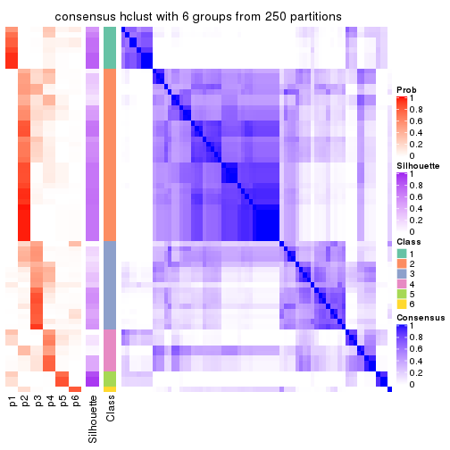
Heatmaps for the membership of samples in all partitions to see how consistent they are:
membership_heatmap(res, k = 2)
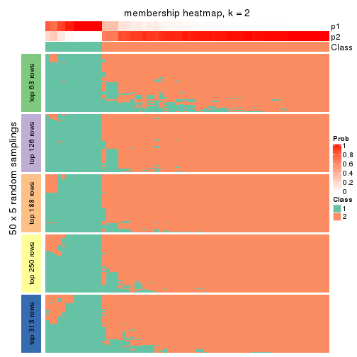
membership_heatmap(res, k = 3)
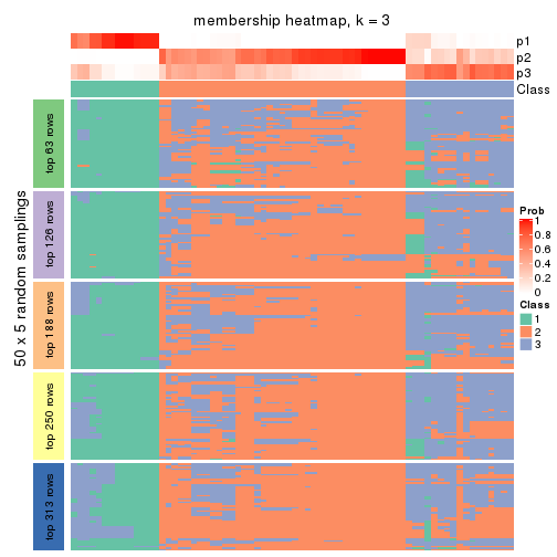
membership_heatmap(res, k = 4)
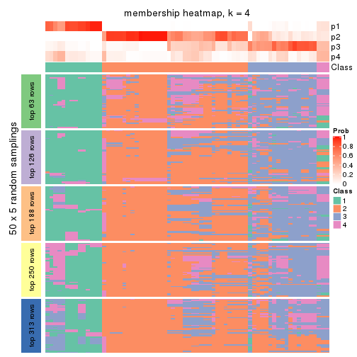
membership_heatmap(res, k = 5)
membership_heatmap(res, k = 6)
As soon as we have had the classes for columns, we can look for signatures which are significantly different between classes which can be candidate marks for certain classes. Following are the heatmaps for signatures.
Signature heatmaps where rows are scaled:
get_signatures(res, k = 2)
get_signatures(res, k = 3)
get_signatures(res, k = 4)
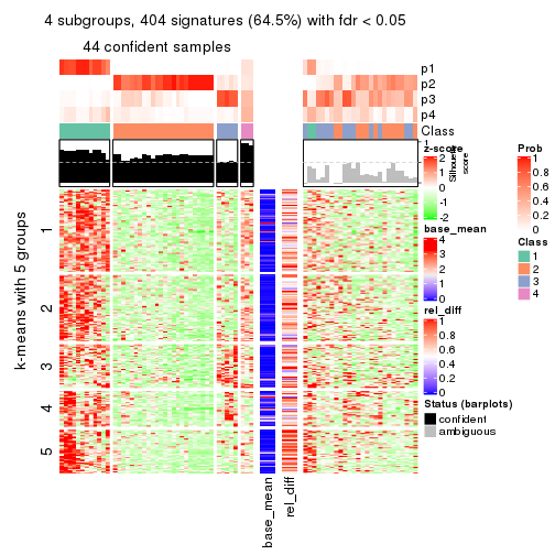
get_signatures(res, k = 5)
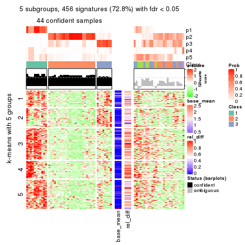
get_signatures(res, k = 6)
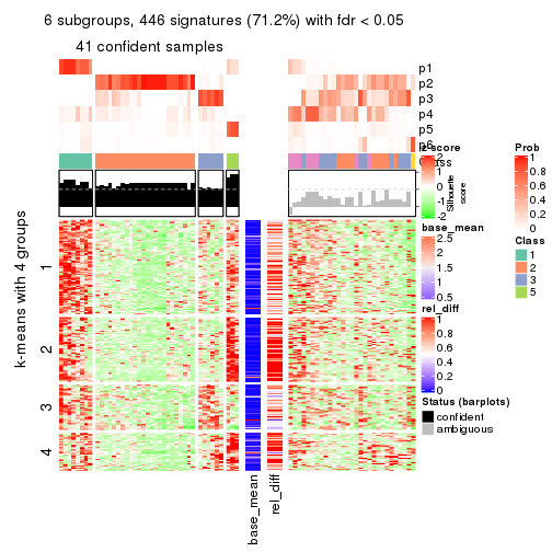
Signature heatmaps where rows are not scaled:
get_signatures(res, k = 2, scale_rows = FALSE)
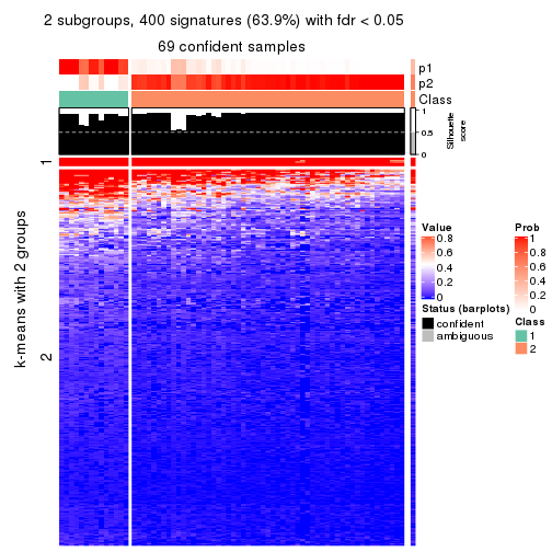
get_signatures(res, k = 3, scale_rows = FALSE)
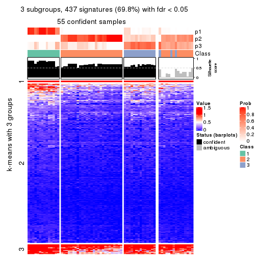
get_signatures(res, k = 4, scale_rows = FALSE)
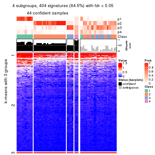
get_signatures(res, k = 5, scale_rows = FALSE)
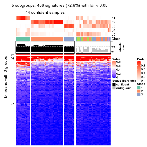
get_signatures(res, k = 6, scale_rows = FALSE)
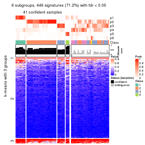
Compare the overlap of signatures from different k:
compare_signatures(res)
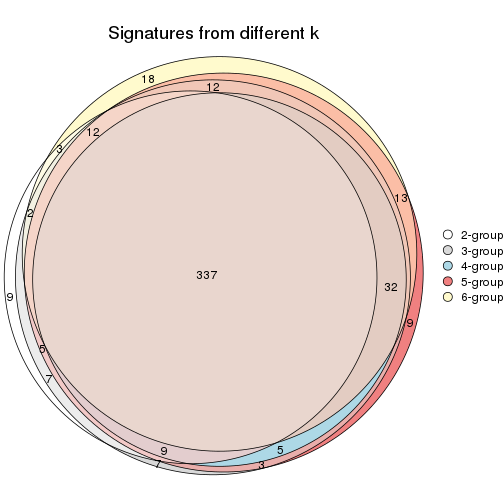
get_signature() returns a data frame invisibly. TO get the list of signatures, the function
call should be assigned to a variable explicitly. In following code, if plot argument is set
to FALSE, no heatmap is plotted while only the differential analysis is performed.
# code only for demonstration
tb = get_signature(res, k = ..., plot = FALSE)
An example of the output of tb is:
#>   which_row         fdr    mean_1    mean_2 scaled_mean_1 scaled_mean_2 km
#> 1        38 0.042760348  8.373488  9.131774    -0.5533452     0.5164555  1
#> 2        40 0.018707592  7.106213  8.469186    -0.6173731     0.5762149  1
#> 3        55 0.019134737 10.221463 11.207825    -0.6159697     0.5749050  1
#> 4        59 0.006059896  5.921854  7.869574    -0.6899429     0.6439467  1
#> 5        60 0.018055526  8.928898 10.211722    -0.6204761     0.5791110  1
#> 6        98 0.009384629 15.714769 14.887706     0.6635654    -0.6193277  2
...
The columns in tb are:
which_row: row indices corresponding to the input matrix.fdr: FDR for the differential test. mean_x: The mean value in group x.scaled_mean_x: The mean value in group x after rows are scaled.km: Row groups if k-means clustering is applied to rows.UMAP plot which shows how samples are separated.
dimension_reduction(res, k = 2, method = "UMAP")
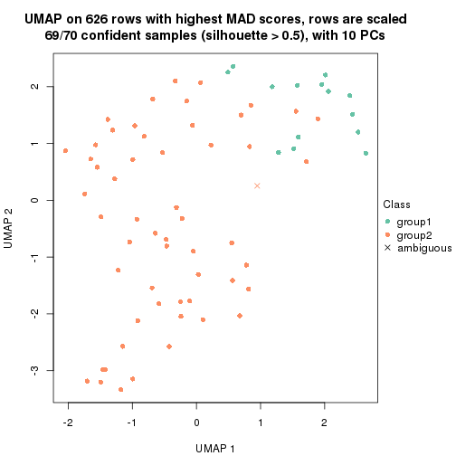
dimension_reduction(res, k = 3, method = "UMAP")
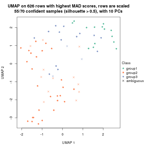
dimension_reduction(res, k = 4, method = "UMAP")
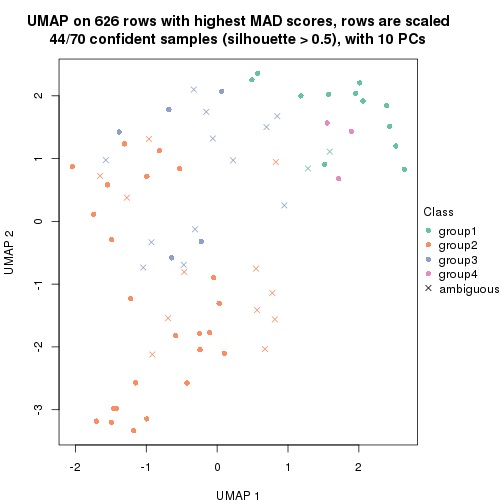
dimension_reduction(res, k = 5, method = "UMAP")
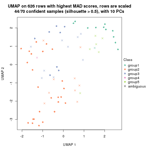
dimension_reduction(res, k = 6, method = "UMAP")
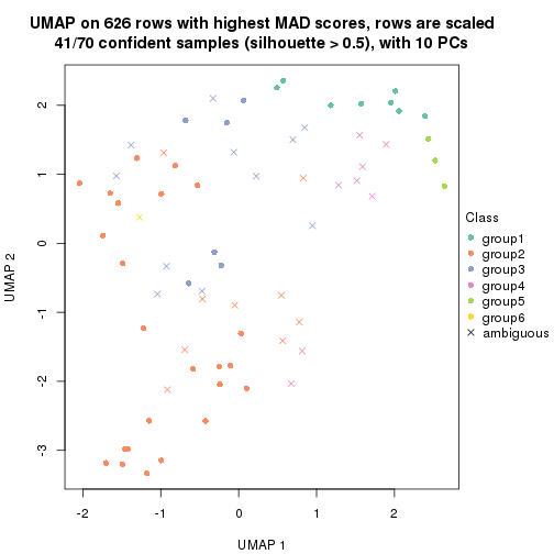
Following heatmap shows how subgroups are split when increasing k:
collect_classes(res)
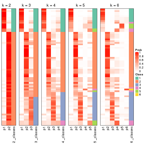
If matrix rows can be associated to genes, consider to use functional_enrichment(res,
...) to perform function enrichment for the signature genes. See this vignette for more detailed explanations.
The object with results only for a single top-value method and a single partition method can be extracted as:
res = res_list["MAD", "kmeans"]
# you can also extract it by
# res = res_list["MAD:kmeans"]
A summary of res and all the functions that can be applied to it:
res
#> A 'ConsensusPartition' object with k = 2, 3, 4, 5, 6.
#>   On a matrix with 626 rows and 70 columns.
#>   Top rows (63, 126, 188, 250, 313) are extracted by 'MAD' method.
#>   Subgroups are detected by 'kmeans' method.
#>   Performed in total 1250 partitions by row resampling.
#>   Best k for subgroups seems to be 3.
#>
#> Following methods can be applied to this 'ConsensusPartition' object:
#>  [1] "cola_report"             "collect_classes"         "collect_plots"
#>  [4] "collect_stats"           "colnames"                "compare_signatures"
#>  [7] "consensus_heatmap"       "dimension_reduction"     "functional_enrichment"
#> [10] "get_anno_col"            "get_anno"                "get_classes"
#> [13] "get_consensus"           "get_matrix"              "get_membership"
#> [16] "get_param"               "get_signatures"          "get_stats"
#> [19] "is_best_k"               "is_stable_k"             "membership_heatmap"
#> [22] "ncol"                    "nrow"                    "plot_ecdf"
#> [25] "rownames"                "select_partition_number" "show"
#> [28] "suggest_best_k"          "test_to_known_factors"
collect_plots() function collects all the plots made from res for all k (number of partitions)
into one single page to provide an easy and fast comparison between different k.
collect_plots(res)
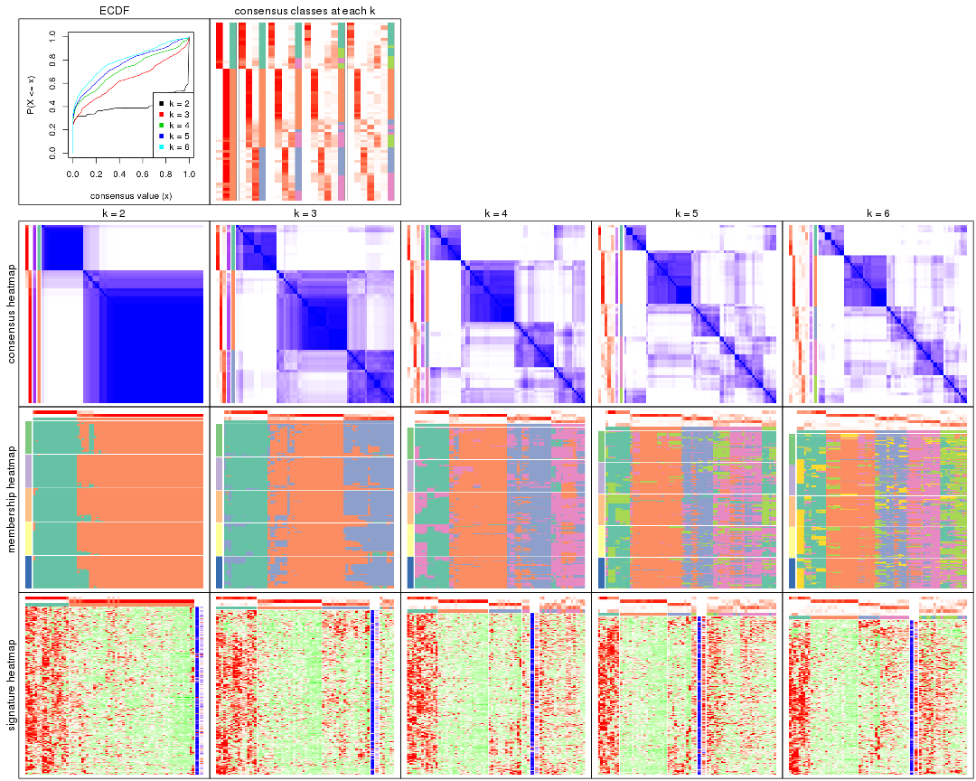
The plots are:
k and the heatmap of
predicted classes for each k.k.k.k.All the plots in panels can be made by individual functions and they are plotted later in this section.
select_partition_number() produces several plots showing different
statistics for choosing “optimized” k. There are following statistics:
k;k, the area increased is defined as \(A_k - A_{k-1}\).The detailed explanations of these statistics can be found in the cola vignette.
Generally speaking, lower PAC score, higher mean silhouette score or higher
concordance corresponds to better partition. Rand index and Jaccard index
measure how similar the current partition is compared to partition with k-1.
If they are too similar, we won't accept k is better than k-1.
select_partition_number(res)
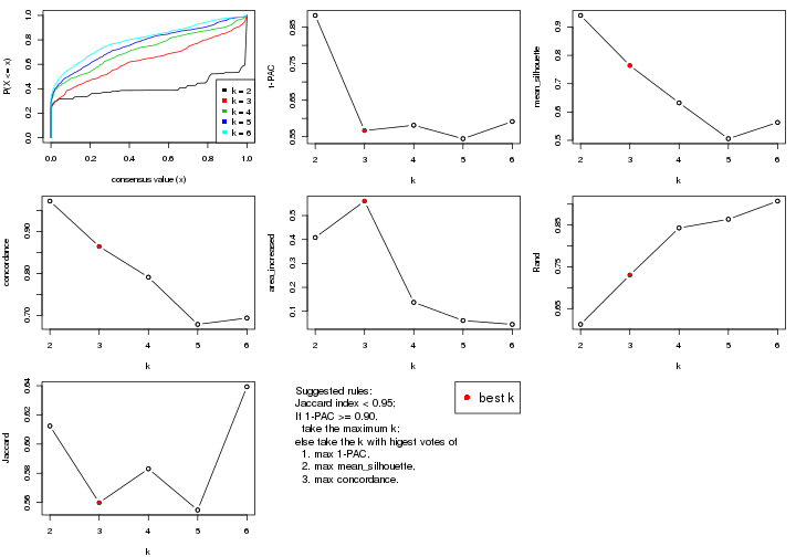
The numeric values for all these statistics can be obtained by get_stats().
get_stats(res)
#>   k 1-PAC mean_silhouette concordance area_increased  Rand Jaccard
#> 2 2 0.882           0.941       0.972         0.4080 0.612   0.612
#> 3 3 0.567           0.764       0.864         0.5602 0.730   0.560
#> 4 4 0.581           0.632       0.791         0.1375 0.843   0.583
#> 5 5 0.545           0.506       0.679         0.0614 0.864   0.555
#> 6 6 0.592           0.563       0.694         0.0454 0.907   0.639
suggest_best_k() suggests the best \(k\) based on these statistics. The rules are as follows:
suggest_best_k(res)
#> [1] 3
Following shows the table of the partitions (You need to click the show/hide
code output link to see it). The membership matrix (columns with name p*)
is inferred by
clue::cl_consensus()
function with the SE method. Basically the value in the membership matrix
represents the probability to belong to a certain group. The finall class
label for an item is determined with the group with highest probability it
belongs to.
In get_classes() function, the entropy is calculated from the membership
matrix and the silhouette score is calculated from the consensus matrix.
cbind(get_classes(res, k = 2), get_membership(res, k = 2))
#>           class entropy silhouette    p1    p2
#> SRR837437     2  0.0000      0.964 0.000 1.000
#> SRR837438     2  0.6973      0.785 0.188 0.812
#> SRR837439     2  0.0000      0.964 0.000 1.000
#> SRR837440     2  0.0000      0.964 0.000 1.000
#> SRR837441     2  0.0000      0.964 0.000 1.000
#> SRR837442     2  0.0000      0.964 0.000 1.000
#> SRR837443     2  0.0000      0.964 0.000 1.000
#> SRR837444     2  0.0376      0.961 0.004 0.996
#> SRR837445     2  0.0000      0.964 0.000 1.000
#> SRR837446     2  0.0000      0.964 0.000 1.000
#> SRR837447     1  0.0000      0.991 1.000 0.000
#> SRR837448     1  0.0000      0.991 1.000 0.000
#> SRR837449     1  0.0000      0.991 1.000 0.000
#> SRR837450     1  0.0000      0.991 1.000 0.000
#> SRR837451     2  0.0000      0.964 0.000 1.000
#> SRR837452     2  0.0000      0.964 0.000 1.000
#> SRR837453     2  0.0000      0.964 0.000 1.000
#> SRR837454     2  0.0000      0.964 0.000 1.000
#> SRR837455     1  0.0000      0.991 1.000 0.000
#> SRR837456     1  0.0000      0.991 1.000 0.000
#> SRR837457     2  0.0000      0.964 0.000 1.000
#> SRR837458     1  0.0000      0.991 1.000 0.000
#> SRR837459     2  0.0000      0.964 0.000 1.000
#> SRR837460     2  0.0000      0.964 0.000 1.000
#> SRR837461     2  0.0000      0.964 0.000 1.000
#> SRR837462     2  0.9358      0.513 0.352 0.648
#> SRR837463     2  0.7219      0.769 0.200 0.800
#> SRR837464     2  0.0000      0.964 0.000 1.000
#> SRR837465     2  0.2423      0.935 0.040 0.960
#> SRR837466     1  0.0000      0.991 1.000 0.000
#> SRR837467     2  0.0000      0.964 0.000 1.000
#> SRR837468     2  0.8861      0.609 0.304 0.696
#> SRR837469     1  0.0000      0.991 1.000 0.000
#> SRR837470     1  0.0000      0.991 1.000 0.000
#> SRR837471     2  0.0000      0.964 0.000 1.000
#> SRR837472     2  0.0000      0.964 0.000 1.000
#> SRR837473     2  0.2423      0.936 0.040 0.960
#> SRR837474     2  0.0000      0.964 0.000 1.000
#> SRR837475     2  0.0000      0.964 0.000 1.000
#> SRR837476     2  0.0000      0.964 0.000 1.000
#> SRR837477     2  0.7056      0.774 0.192 0.808
#> SRR837478     2  0.0000      0.964 0.000 1.000
#> SRR837479     2  0.0000      0.964 0.000 1.000
#> SRR837480     2  0.0000      0.964 0.000 1.000
#> SRR837481     2  0.0376      0.961 0.004 0.996
#> SRR837482     2  0.8267      0.681 0.260 0.740
#> SRR837483     1  0.0376      0.988 0.996 0.004
#> SRR837484     2  0.0000      0.964 0.000 1.000
#> SRR837485     2  0.0000      0.964 0.000 1.000
#> SRR837486     2  0.1633      0.948 0.024 0.976
#> SRR837487     2  0.0000      0.964 0.000 1.000
#> SRR837488     2  0.0000      0.964 0.000 1.000
#> SRR837489     2  0.0000      0.964 0.000 1.000
#> SRR837490     2  0.0000      0.964 0.000 1.000
#> SRR837491     2  0.0000      0.964 0.000 1.000
#> SRR837492     2  0.0672      0.959 0.008 0.992
#> SRR837493     2  0.7376      0.759 0.208 0.792
#> SRR837494     2  0.0000      0.964 0.000 1.000
#> SRR837495     2  0.0000      0.964 0.000 1.000
#> SRR837496     1  0.0000      0.991 1.000 0.000
#> SRR837497     1  0.0000      0.991 1.000 0.000
#> SRR837498     1  0.0000      0.991 1.000 0.000
#> SRR837499     1  0.0000      0.991 1.000 0.000
#> SRR837500     1  0.0938      0.981 0.988 0.012
#> SRR837501     2  0.0000      0.964 0.000 1.000
#> SRR837502     1  0.5294      0.853 0.880 0.120
#> SRR837503     1  0.0000      0.991 1.000 0.000
#> SRR837504     2  0.0000      0.964 0.000 1.000
#> SRR837505     2  0.0000      0.964 0.000 1.000
#> SRR837506     2  0.0000      0.964 0.000 1.000
cbind(get_classes(res, k = 3), get_membership(res, k = 3))
#>           class entropy silhouette    p1    p2    p3
#> SRR837437     2  0.1753     0.8414 0.000 0.952 0.048
#> SRR837438     3  0.4379     0.7736 0.060 0.072 0.868
#> SRR837439     2  0.5621     0.4398 0.000 0.692 0.308
#> SRR837440     3  0.5859     0.6856 0.000 0.344 0.656
#> SRR837441     2  0.5591     0.4474 0.000 0.696 0.304
#> SRR837442     2  0.0424     0.8637 0.000 0.992 0.008
#> SRR837443     3  0.5560     0.7346 0.000 0.300 0.700
#> SRR837444     3  0.2774     0.7950 0.008 0.072 0.920
#> SRR837445     2  0.5560     0.5662 0.000 0.700 0.300
#> SRR837446     3  0.5058     0.7634 0.000 0.244 0.756
#> SRR837447     1  0.0592     0.9076 0.988 0.000 0.012
#> SRR837448     1  0.2261     0.8845 0.932 0.000 0.068
#> SRR837449     1  0.2261     0.9024 0.932 0.000 0.068
#> SRR837450     1  0.2261     0.8845 0.932 0.000 0.068
#> SRR837451     2  0.0424     0.8637 0.000 0.992 0.008
#> SRR837452     2  0.0000     0.8623 0.000 1.000 0.000
#> SRR837453     2  0.0424     0.8637 0.000 0.992 0.008
#> SRR837454     2  0.0000     0.8623 0.000 1.000 0.000
#> SRR837455     1  0.0592     0.9078 0.988 0.000 0.012
#> SRR837456     1  0.0592     0.9078 0.988 0.000 0.012
#> SRR837457     2  0.0424     0.8637 0.000 0.992 0.008
#> SRR837458     1  0.0747     0.9073 0.984 0.000 0.016
#> SRR837459     2  0.0424     0.8637 0.000 0.992 0.008
#> SRR837460     2  0.0424     0.8637 0.000 0.992 0.008
#> SRR837461     3  0.6026     0.6369 0.000 0.376 0.624
#> SRR837462     3  0.2998     0.7503 0.068 0.016 0.916
#> SRR837463     3  0.4379     0.7736 0.060 0.072 0.868
#> SRR837464     3  0.4178     0.7947 0.000 0.172 0.828
#> SRR837465     3  0.6570     0.5781 0.028 0.292 0.680
#> SRR837466     1  0.2261     0.8845 0.932 0.000 0.068
#> SRR837467     2  0.1289     0.8519 0.000 0.968 0.032
#> SRR837468     3  0.2749     0.7499 0.064 0.012 0.924
#> SRR837469     1  0.0424     0.9077 0.992 0.000 0.008
#> SRR837470     1  0.0424     0.9077 0.992 0.000 0.008
#> SRR837471     2  0.0237     0.8627 0.000 0.996 0.004
#> SRR837472     2  0.0000     0.8623 0.000 1.000 0.000
#> SRR837473     2  0.5378     0.6491 0.008 0.756 0.236
#> SRR837474     2  0.0237     0.8627 0.000 0.996 0.004
#> SRR837475     2  0.0000     0.8623 0.000 1.000 0.000
#> SRR837476     2  0.0747     0.8617 0.000 0.984 0.016
#> SRR837477     2  0.8533     0.2762 0.104 0.536 0.360
#> SRR837478     2  0.2959     0.7927 0.000 0.900 0.100
#> SRR837479     3  0.4452     0.7908 0.000 0.192 0.808
#> SRR837480     2  0.4062     0.7309 0.000 0.836 0.164
#> SRR837481     3  0.4002     0.8008 0.000 0.160 0.840
#> SRR837482     3  0.3028     0.7707 0.048 0.032 0.920
#> SRR837483     1  0.5968     0.5558 0.636 0.000 0.364
#> SRR837484     2  0.6180     0.0264 0.000 0.584 0.416
#> SRR837485     3  0.6267     0.4193 0.000 0.452 0.548
#> SRR837486     3  0.2959     0.8025 0.000 0.100 0.900
#> SRR837487     2  0.0424     0.8637 0.000 0.992 0.008
#> SRR837488     2  0.0424     0.8637 0.000 0.992 0.008
#> SRR837489     2  0.0237     0.8627 0.000 0.996 0.004
#> SRR837490     2  0.0000     0.8623 0.000 1.000 0.000
#> SRR837491     2  0.5733     0.5158 0.000 0.676 0.324
#> SRR837492     2  0.4931     0.6679 0.000 0.768 0.232
#> SRR837493     3  0.4379     0.7736 0.060 0.072 0.868
#> SRR837494     2  0.1289     0.8519 0.000 0.968 0.032
#> SRR837495     2  0.4346     0.7225 0.000 0.816 0.184
#> SRR837496     1  0.2165     0.9053 0.936 0.000 0.064
#> SRR837497     1  0.2165     0.9010 0.936 0.000 0.064
#> SRR837498     1  0.2261     0.9002 0.932 0.000 0.068
#> SRR837499     1  0.2796     0.8896 0.908 0.000 0.092
#> SRR837500     1  0.6012     0.7497 0.748 0.032 0.220
#> SRR837501     3  0.3482     0.8045 0.000 0.128 0.872
#> SRR837502     1  0.6994     0.4010 0.556 0.020 0.424
#> SRR837503     1  0.2356     0.9005 0.928 0.000 0.072
#> SRR837504     3  0.5810     0.6770 0.000 0.336 0.664
#> SRR837505     3  0.5591     0.7113 0.000 0.304 0.696
#> SRR837506     3  0.5926     0.6415 0.000 0.356 0.644
cbind(get_classes(res, k = 4), get_membership(res, k = 4))
#>           class entropy silhouette    p1    p2    p3    p4
#> SRR837437     2  0.2300     0.8547 0.000 0.924 0.028 0.048
#> SRR837438     4  0.5165     0.1804 0.004 0.004 0.388 0.604
#> SRR837439     2  0.6915     0.3391 0.000 0.592 0.196 0.212
#> SRR837440     3  0.7110     0.5045 0.000 0.236 0.564 0.200
#> SRR837441     2  0.6819     0.3652 0.000 0.604 0.188 0.208
#> SRR837442     2  0.0672     0.8885 0.000 0.984 0.008 0.008
#> SRR837443     3  0.7062     0.5089 0.000 0.224 0.572 0.204
#> SRR837444     4  0.5050     0.1390 0.000 0.004 0.408 0.588
#> SRR837445     4  0.6370     0.5484 0.000 0.280 0.100 0.620
#> SRR837446     3  0.3587     0.6950 0.000 0.088 0.860 0.052
#> SRR837447     1  0.0707     0.8072 0.980 0.000 0.000 0.020
#> SRR837448     1  0.3324     0.7576 0.852 0.000 0.012 0.136
#> SRR837449     1  0.4605     0.6026 0.664 0.000 0.000 0.336
#> SRR837450     1  0.3377     0.7582 0.848 0.000 0.012 0.140
#> SRR837451     2  0.0524     0.8883 0.000 0.988 0.008 0.004
#> SRR837452     2  0.2197     0.8532 0.000 0.916 0.004 0.080
#> SRR837453     2  0.0524     0.8883 0.000 0.988 0.008 0.004
#> SRR837454     2  0.0188     0.8874 0.000 0.996 0.000 0.004
#> SRR837455     1  0.1211     0.8058 0.960 0.000 0.000 0.040
#> SRR837456     1  0.1211     0.8058 0.960 0.000 0.000 0.040
#> SRR837457     2  0.0524     0.8883 0.000 0.988 0.008 0.004
#> SRR837458     1  0.0817     0.8059 0.976 0.000 0.000 0.024
#> SRR837459     2  0.0524     0.8883 0.000 0.988 0.008 0.004
#> SRR837460     2  0.0524     0.8883 0.000 0.988 0.008 0.004
#> SRR837461     3  0.7095     0.4840 0.000 0.260 0.560 0.180
#> SRR837462     3  0.5080     0.2846 0.004 0.000 0.576 0.420
#> SRR837463     3  0.5384     0.2735 0.004 0.008 0.568 0.420
#> SRR837464     3  0.4808     0.5891 0.000 0.028 0.736 0.236
#> SRR837465     4  0.5507     0.4558 0.004 0.064 0.212 0.720
#> SRR837466     1  0.3324     0.7576 0.852 0.000 0.012 0.136
#> SRR837467     2  0.2174     0.8578 0.000 0.928 0.020 0.052
#> SRR837468     3  0.1792     0.6941 0.000 0.000 0.932 0.068
#> SRR837469     1  0.1004     0.8052 0.972 0.000 0.004 0.024
#> SRR837470     1  0.0779     0.8050 0.980 0.000 0.004 0.016
#> SRR837471     2  0.1902     0.8646 0.000 0.932 0.004 0.064
#> SRR837472     2  0.1489     0.8730 0.000 0.952 0.004 0.044
#> SRR837473     4  0.5384     0.5569 0.004 0.292 0.028 0.676
#> SRR837474     2  0.1824     0.8675 0.000 0.936 0.004 0.060
#> SRR837475     2  0.1661     0.8693 0.000 0.944 0.004 0.052
#> SRR837476     2  0.0469     0.8869 0.000 0.988 0.000 0.012
#> SRR837477     4  0.7412     0.4800 0.012 0.232 0.188 0.568
#> SRR837478     2  0.5850     0.6122 0.000 0.700 0.184 0.116
#> SRR837479     3  0.1388     0.7051 0.000 0.012 0.960 0.028
#> SRR837480     2  0.6587     0.4422 0.000 0.596 0.292 0.112
#> SRR837481     3  0.1388     0.7051 0.000 0.012 0.960 0.028
#> SRR837482     3  0.1978     0.6869 0.004 0.000 0.928 0.068
#> SRR837483     4  0.7519     0.0574 0.312 0.000 0.208 0.480
#> SRR837484     3  0.5250     0.2683 0.000 0.440 0.552 0.008
#> SRR837485     3  0.4452     0.5633 0.000 0.260 0.732 0.008
#> SRR837486     3  0.1635     0.7021 0.000 0.008 0.948 0.044
#> SRR837487     2  0.0937     0.8883 0.000 0.976 0.012 0.012
#> SRR837488     2  0.0524     0.8883 0.000 0.988 0.008 0.004
#> SRR837489     2  0.2466     0.8484 0.000 0.900 0.004 0.096
#> SRR837490     2  0.0188     0.8883 0.000 0.996 0.004 0.000
#> SRR837491     4  0.6584     0.4528 0.000 0.336 0.096 0.568
#> SRR837492     4  0.5717     0.5116 0.000 0.324 0.044 0.632
#> SRR837493     4  0.5212     0.1398 0.004 0.004 0.404 0.588
#> SRR837494     2  0.1975     0.8605 0.000 0.936 0.016 0.048
#> SRR837495     4  0.5807     0.4682 0.000 0.344 0.044 0.612
#> SRR837496     1  0.4898     0.5198 0.584 0.000 0.000 0.416
#> SRR837497     1  0.4584     0.6659 0.696 0.000 0.004 0.300
#> SRR837498     1  0.4621     0.6689 0.708 0.000 0.008 0.284
#> SRR837499     4  0.5143    -0.2646 0.456 0.000 0.004 0.540
#> SRR837500     4  0.4652     0.3672 0.220 0.004 0.020 0.756
#> SRR837501     3  0.2089     0.7117 0.000 0.020 0.932 0.048
#> SRR837502     4  0.4820     0.4408 0.168 0.000 0.060 0.772
#> SRR837503     1  0.4967     0.4528 0.548 0.000 0.000 0.452
#> SRR837504     3  0.4957     0.6484 0.000 0.204 0.748 0.048
#> SRR837505     3  0.2282     0.7157 0.000 0.052 0.924 0.024
#> SRR837506     3  0.2473     0.6980 0.000 0.080 0.908 0.012
cbind(get_classes(res, k = 5), get_membership(res, k = 5))
#>           class entropy silhouette    p1    p2    p3    p4    p5
#> SRR837437     2  0.3973     0.7294 0.000 0.792 0.036 0.164 0.008
#> SRR837438     4  0.4103     0.4397 0.000 0.008 0.136 0.796 0.060
#> SRR837439     4  0.6202     0.2133 0.000 0.408 0.108 0.476 0.008
#> SRR837440     4  0.7228     0.2239 0.000 0.252 0.276 0.444 0.028
#> SRR837441     4  0.6244     0.1898 0.000 0.416 0.112 0.464 0.008
#> SRR837442     2  0.2100     0.8619 0.000 0.924 0.016 0.048 0.012
#> SRR837443     4  0.6809     0.2428 0.000 0.224 0.280 0.484 0.012
#> SRR837444     4  0.3841     0.4250 0.000 0.000 0.188 0.780 0.032
#> SRR837445     4  0.7072     0.3537 0.000 0.124 0.092 0.560 0.224
#> SRR837446     3  0.4864     0.5812 0.000 0.060 0.768 0.116 0.056
#> SRR837447     1  0.4182     0.5750 0.644 0.000 0.004 0.000 0.352
#> SRR837448     1  0.0324     0.5372 0.992 0.000 0.000 0.004 0.004
#> SRR837449     5  0.6542     0.4462 0.360 0.000 0.004 0.176 0.460
#> SRR837450     1  0.0324     0.5372 0.992 0.000 0.000 0.004 0.004
#> SRR837451     2  0.0955     0.8742 0.000 0.968 0.004 0.000 0.028
#> SRR837452     2  0.3209     0.8325 0.000 0.860 0.004 0.060 0.076
#> SRR837453     2  0.0955     0.8742 0.000 0.968 0.004 0.000 0.028
#> SRR837454     2  0.0955     0.8734 0.000 0.968 0.000 0.004 0.028
#> SRR837455     1  0.4449     0.5449 0.604 0.000 0.004 0.004 0.388
#> SRR837456     1  0.4449     0.5449 0.604 0.000 0.004 0.004 0.388
#> SRR837457     2  0.0955     0.8742 0.000 0.968 0.004 0.000 0.028
#> SRR837458     1  0.4434     0.5787 0.640 0.000 0.004 0.008 0.348
#> SRR837459     2  0.0955     0.8742 0.000 0.968 0.004 0.000 0.028
#> SRR837460     2  0.0955     0.8742 0.000 0.968 0.004 0.000 0.028
#> SRR837461     4  0.7508     0.1791 0.000 0.240 0.308 0.408 0.044
#> SRR837462     4  0.5441     0.2586 0.000 0.000 0.324 0.596 0.080
#> SRR837463     4  0.5419     0.3205 0.000 0.012 0.284 0.640 0.064
#> SRR837464     4  0.5968     0.0700 0.000 0.020 0.440 0.480 0.060
#> SRR837465     4  0.3796     0.4289 0.000 0.016 0.076 0.832 0.076
#> SRR837466     1  0.0162     0.5378 0.996 0.000 0.000 0.000 0.004
#> SRR837467     2  0.3757     0.7558 0.000 0.808 0.024 0.156 0.012
#> SRR837468     3  0.4498     0.5792 0.000 0.000 0.756 0.112 0.132
#> SRR837469     1  0.4974     0.5456 0.640 0.000 0.004 0.040 0.316
#> SRR837470     1  0.4956     0.5482 0.644 0.000 0.004 0.040 0.312
#> SRR837471     2  0.3119     0.8335 0.000 0.860 0.000 0.072 0.068
#> SRR837472     2  0.2863     0.8412 0.000 0.876 0.000 0.060 0.064
#> SRR837473     4  0.6661     0.2685 0.000 0.172 0.020 0.532 0.276
#> SRR837474     2  0.2863     0.8454 0.000 0.876 0.000 0.064 0.060
#> SRR837475     2  0.2853     0.8361 0.000 0.876 0.000 0.052 0.072
#> SRR837476     2  0.1768     0.8640 0.000 0.924 0.000 0.072 0.004
#> SRR837477     4  0.8496     0.1348 0.032 0.068 0.260 0.360 0.280
#> SRR837478     2  0.7895     0.0677 0.000 0.440 0.276 0.136 0.148
#> SRR837479     3  0.2740     0.6377 0.000 0.004 0.888 0.064 0.044
#> SRR837480     3  0.7865     0.1109 0.000 0.360 0.380 0.132 0.128
#> SRR837481     3  0.2729     0.6354 0.000 0.000 0.884 0.056 0.060
#> SRR837482     3  0.3181     0.6384 0.000 0.000 0.856 0.072 0.072
#> SRR837483     5  0.8319     0.3318 0.156 0.000 0.216 0.260 0.368
#> SRR837484     3  0.5415     0.1255 0.000 0.464 0.492 0.028 0.016
#> SRR837485     3  0.4902     0.5006 0.000 0.268 0.684 0.032 0.016
#> SRR837486     3  0.2592     0.6474 0.000 0.000 0.892 0.056 0.052
#> SRR837487     2  0.2165     0.8703 0.000 0.924 0.016 0.024 0.036
#> SRR837488     2  0.0955     0.8742 0.000 0.968 0.004 0.000 0.028
#> SRR837489     2  0.3008     0.8429 0.000 0.868 0.004 0.092 0.036
#> SRR837490     2  0.0955     0.8746 0.000 0.968 0.000 0.028 0.004
#> SRR837491     4  0.5043     0.4655 0.000 0.208 0.028 0.716 0.048
#> SRR837492     4  0.7360     0.2490 0.000 0.144 0.076 0.488 0.292
#> SRR837493     4  0.4184     0.4373 0.000 0.008 0.132 0.792 0.068
#> SRR837494     2  0.3404     0.7811 0.000 0.840 0.024 0.124 0.012
#> SRR837495     4  0.7492     0.2843 0.000 0.196 0.068 0.476 0.260
#> SRR837496     1  0.6460    -0.5219 0.412 0.000 0.000 0.180 0.408
#> SRR837497     5  0.6344     0.3876 0.400 0.000 0.000 0.160 0.440
#> SRR837498     5  0.6404     0.3443 0.372 0.000 0.004 0.152 0.472
#> SRR837499     5  0.6610     0.5290 0.224 0.000 0.000 0.340 0.436
#> SRR837500     4  0.5873    -0.2544 0.068 0.012 0.000 0.508 0.412
#> SRR837501     3  0.3648     0.6124 0.000 0.000 0.824 0.084 0.092
#> SRR837502     4  0.5590    -0.1627 0.056 0.004 0.004 0.556 0.380
#> SRR837503     5  0.6670     0.5510 0.308 0.000 0.000 0.256 0.436
#> SRR837504     3  0.6938     0.2867 0.000 0.272 0.520 0.172 0.036
#> SRR837505     3  0.3566     0.6462 0.000 0.032 0.848 0.032 0.088
#> SRR837506     3  0.3628     0.6529 0.000 0.048 0.836 0.012 0.104
cbind(get_classes(res, k = 6), get_membership(res, k = 6))
#>           class entropy silhouette    p1    p2    p3    p4    p5    p6
#> SRR837437     2   0.445    0.65652 0.000 0.728 0.028 0.204 0.004 0.036
#> SRR837438     4   0.296    0.59291 0.000 0.000 0.020 0.840 0.132 0.008
#> SRR837439     4   0.512    0.58621 0.000 0.280 0.032 0.644 0.020 0.024
#> SRR837440     4   0.525    0.63040 0.000 0.208 0.108 0.660 0.004 0.020
#> SRR837441     4   0.514    0.58249 0.000 0.284 0.032 0.640 0.020 0.024
#> SRR837442     2   0.336    0.80714 0.000 0.852 0.016 0.072 0.024 0.036
#> SRR837443     4   0.543    0.63495 0.000 0.204 0.108 0.656 0.012 0.020
#> SRR837444     4   0.422    0.54981 0.000 0.000 0.076 0.752 0.160 0.012
#> SRR837445     5   0.730    0.32073 0.000 0.056 0.112 0.240 0.504 0.088
#> SRR837446     3   0.475    0.57771 0.000 0.036 0.764 0.084 0.084 0.032
#> SRR837447     1   0.146    0.65696 0.940 0.000 0.000 0.000 0.044 0.016
#> SRR837448     1   0.386    0.53144 0.520 0.000 0.000 0.000 0.000 0.480
#> SRR837449     1   0.515    0.22363 0.544 0.000 0.000 0.080 0.372 0.004
#> SRR837450     1   0.386    0.53144 0.520 0.000 0.000 0.000 0.000 0.480
#> SRR837451     2   0.139    0.83324 0.000 0.932 0.000 0.000 0.000 0.068
#> SRR837452     2   0.388    0.78481 0.000 0.788 0.008 0.028 0.156 0.020
#> SRR837453     2   0.139    0.83324 0.000 0.932 0.000 0.000 0.000 0.068
#> SRR837454     2   0.164    0.83198 0.000 0.924 0.000 0.000 0.008 0.068
#> SRR837455     1   0.221    0.64721 0.900 0.000 0.000 0.004 0.072 0.024
#> SRR837456     1   0.221    0.64721 0.900 0.000 0.000 0.004 0.072 0.024
#> SRR837457     2   0.139    0.83324 0.000 0.932 0.000 0.000 0.000 0.068
#> SRR837458     1   0.201    0.65252 0.920 0.000 0.000 0.012 0.032 0.036
#> SRR837459     2   0.139    0.83324 0.000 0.932 0.000 0.000 0.000 0.068
#> SRR837460     2   0.139    0.83324 0.000 0.932 0.000 0.000 0.000 0.068
#> SRR837461     4   0.514    0.62981 0.000 0.184 0.112 0.676 0.000 0.028
#> SRR837462     4   0.371    0.59376 0.004 0.000 0.088 0.820 0.024 0.064
#> SRR837463     4   0.329    0.61372 0.004 0.000 0.076 0.848 0.020 0.052
#> SRR837464     4   0.384    0.58729 0.000 0.012 0.148 0.784 0.000 0.056
#> SRR837465     4   0.318    0.53815 0.000 0.004 0.004 0.792 0.196 0.004
#> SRR837466     1   0.386    0.53144 0.520 0.000 0.000 0.000 0.000 0.480
#> SRR837467     2   0.428    0.65667 0.000 0.732 0.020 0.212 0.004 0.032
#> SRR837468     3   0.680    0.46833 0.012 0.000 0.492 0.216 0.048 0.232
#> SRR837469     1   0.482    0.61394 0.752 0.000 0.016 0.072 0.052 0.108
#> SRR837470     1   0.471    0.61839 0.760 0.000 0.016 0.068 0.048 0.108
#> SRR837471     2   0.403    0.77161 0.000 0.768 0.000 0.032 0.168 0.032
#> SRR837472     2   0.370    0.78481 0.000 0.792 0.000 0.020 0.156 0.032
#> SRR837473     5   0.581    0.48938 0.004 0.084 0.024 0.160 0.672 0.056
#> SRR837474     2   0.396    0.78895 0.000 0.784 0.000 0.036 0.144 0.036
#> SRR837475     2   0.395    0.77364 0.000 0.772 0.000 0.016 0.164 0.048
#> SRR837476     2   0.243    0.82718 0.000 0.892 0.000 0.072 0.020 0.016
#> SRR837477     5   0.634    0.23105 0.000 0.028 0.316 0.040 0.532 0.084
#> SRR837478     3   0.728    0.12362 0.000 0.244 0.408 0.016 0.268 0.064
#> SRR837479     3   0.246    0.61970 0.000 0.008 0.900 0.012 0.052 0.028
#> SRR837480     3   0.696    0.23434 0.000 0.184 0.492 0.016 0.244 0.064
#> SRR837481     3   0.239    0.62222 0.000 0.008 0.904 0.012 0.048 0.028
#> SRR837482     3   0.481    0.59673 0.004 0.000 0.732 0.132 0.036 0.096
#> SRR837483     5   0.842    0.11213 0.152 0.000 0.192 0.160 0.384 0.112
#> SRR837484     3   0.549    0.29482 0.000 0.372 0.540 0.056 0.004 0.028
#> SRR837485     3   0.495    0.53066 0.000 0.220 0.692 0.048 0.012 0.028
#> SRR837486     3   0.402    0.62691 0.000 0.000 0.788 0.084 0.024 0.104
#> SRR837487     2   0.291    0.83169 0.000 0.880 0.024 0.028 0.052 0.016
#> SRR837488     2   0.153    0.83252 0.000 0.928 0.000 0.004 0.000 0.068
#> SRR837489     2   0.460    0.75984 0.000 0.744 0.000 0.104 0.116 0.036
#> SRR837490     2   0.204    0.83791 0.000 0.920 0.000 0.028 0.032 0.020
#> SRR837491     4   0.599    0.43955 0.000 0.152 0.004 0.588 0.220 0.036
#> SRR837492     5   0.623    0.47688 0.000 0.068 0.088 0.108 0.656 0.080
#> SRR837493     4   0.292    0.59412 0.000 0.000 0.020 0.844 0.128 0.008
#> SRR837494     2   0.380    0.72395 0.000 0.788 0.020 0.152 0.000 0.040
#> SRR837495     5   0.692    0.43894 0.000 0.088 0.108 0.136 0.588 0.080
#> SRR837496     5   0.575   -0.00218 0.344 0.000 0.004 0.036 0.544 0.072
#> SRR837497     1   0.593    0.22327 0.464 0.000 0.008 0.064 0.424 0.040
#> SRR837498     1   0.670    0.34164 0.488 0.000 0.008 0.132 0.304 0.068
#> SRR837499     5   0.549    0.20947 0.288 0.000 0.004 0.128 0.576 0.004
#> SRR837500     5   0.440    0.45097 0.100 0.000 0.000 0.172 0.724 0.004
#> SRR837501     3   0.567    0.54048 0.000 0.004 0.616 0.168 0.020 0.192
#> SRR837502     5   0.434    0.45881 0.040 0.000 0.004 0.260 0.692 0.004
#> SRR837503     5   0.549    0.09722 0.324 0.000 0.004 0.072 0.576 0.024
#> SRR837504     4   0.683    0.06026 0.000 0.240 0.356 0.356 0.000 0.048
#> SRR837505     3   0.538    0.59417 0.000 0.020 0.672 0.108 0.016 0.184
#> SRR837506     3   0.520    0.61824 0.000 0.024 0.692 0.076 0.020 0.188
Heatmaps for the consensus matrix. It visualizes the probability of two samples to be in a same group.
consensus_heatmap(res, k = 2)
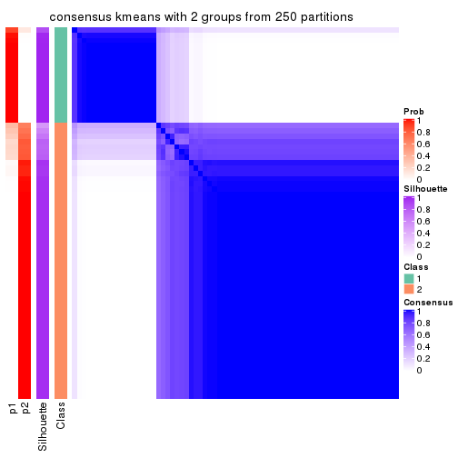
consensus_heatmap(res, k = 3)
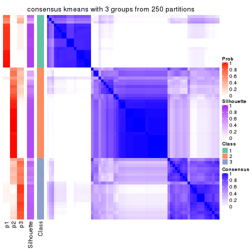
consensus_heatmap(res, k = 4)
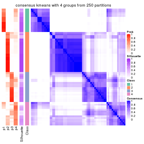
consensus_heatmap(res, k = 5)
consensus_heatmap(res, k = 6)
Heatmaps for the membership of samples in all partitions to see how consistent they are:
membership_heatmap(res, k = 2)
membership_heatmap(res, k = 3)
membership_heatmap(res, k = 4)
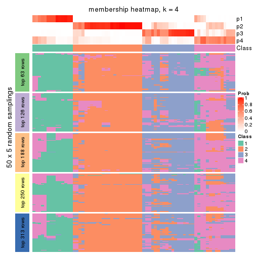
membership_heatmap(res, k = 5)
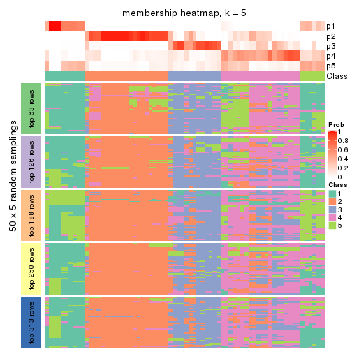
membership_heatmap(res, k = 6)
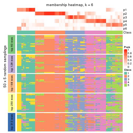
As soon as we have had the classes for columns, we can look for signatures which are significantly different between classes which can be candidate marks for certain classes. Following are the heatmaps for signatures.
Signature heatmaps where rows are scaled:
get_signatures(res, k = 2)
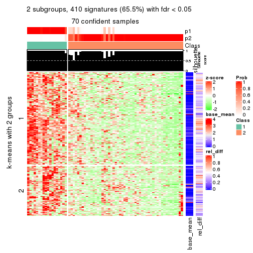
get_signatures(res, k = 3)
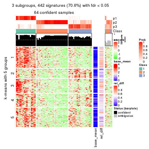
get_signatures(res, k = 4)
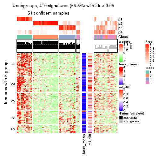
get_signatures(res, k = 5)
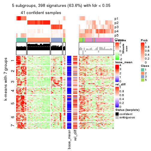
get_signatures(res, k = 6)
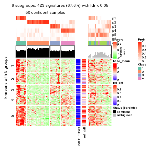
Signature heatmaps where rows are not scaled:
get_signatures(res, k = 2, scale_rows = FALSE)
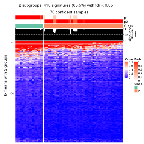
get_signatures(res, k = 3, scale_rows = FALSE)
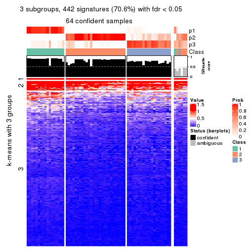
get_signatures(res, k = 4, scale_rows = FALSE)
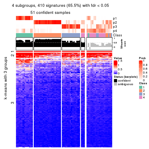
get_signatures(res, k = 5, scale_rows = FALSE)
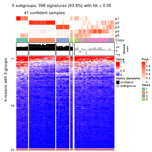
get_signatures(res, k = 6, scale_rows = FALSE)
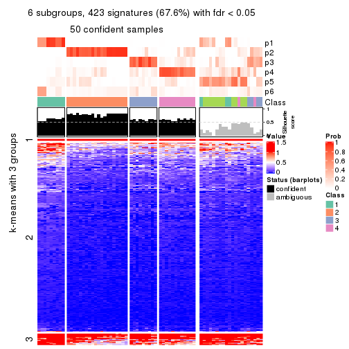
Compare the overlap of signatures from different k:
compare_signatures(res)
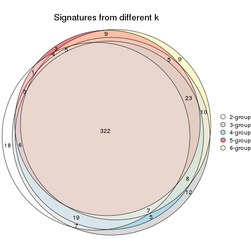
get_signature() returns a data frame invisibly. TO get the list of signatures, the function
call should be assigned to a variable explicitly. In following code, if plot argument is set
to FALSE, no heatmap is plotted while only the differential analysis is performed.
# code only for demonstration
tb = get_signature(res, k = ..., plot = FALSE)
An example of the output of tb is:
#>   which_row         fdr    mean_1    mean_2 scaled_mean_1 scaled_mean_2 km
#> 1        38 0.042760348  8.373488  9.131774    -0.5533452     0.5164555  1
#> 2        40 0.018707592  7.106213  8.469186    -0.6173731     0.5762149  1
#> 3        55 0.019134737 10.221463 11.207825    -0.6159697     0.5749050  1
#> 4        59 0.006059896  5.921854  7.869574    -0.6899429     0.6439467  1
#> 5        60 0.018055526  8.928898 10.211722    -0.6204761     0.5791110  1
#> 6        98 0.009384629 15.714769 14.887706     0.6635654    -0.6193277  2
...
The columns in tb are:
which_row: row indices corresponding to the input matrix.fdr: FDR for the differential test. mean_x: The mean value in group x.scaled_mean_x: The mean value in group x after rows are scaled.km: Row groups if k-means clustering is applied to rows.UMAP plot which shows how samples are separated.
dimension_reduction(res, k = 2, method = "UMAP")
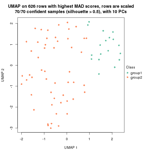
dimension_reduction(res, k = 3, method = "UMAP")
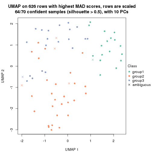
dimension_reduction(res, k = 4, method = "UMAP")
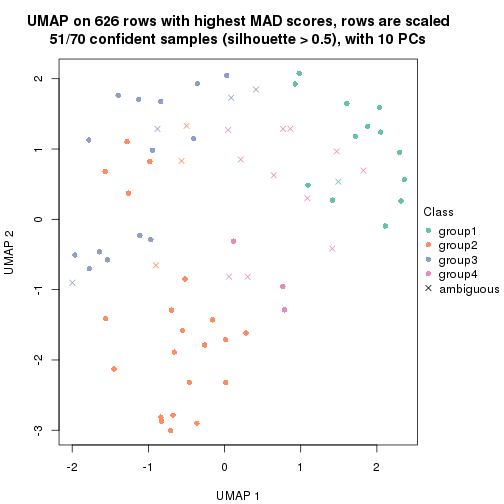
dimension_reduction(res, k = 5, method = "UMAP")
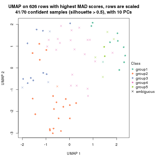
dimension_reduction(res, k = 6, method = "UMAP")
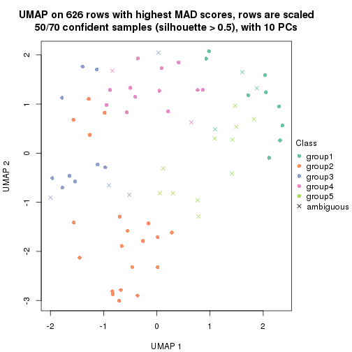
Following heatmap shows how subgroups are split when increasing k:
collect_classes(res)
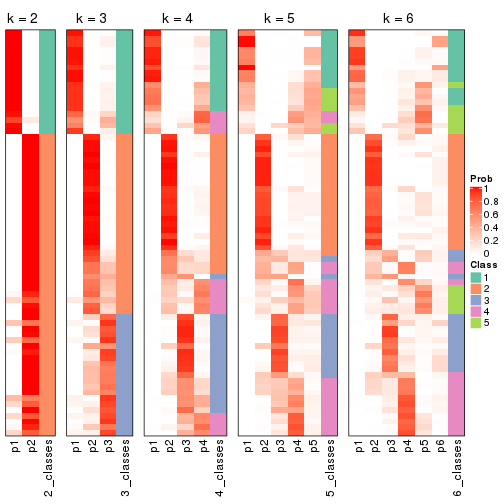
If matrix rows can be associated to genes, consider to use functional_enrichment(res,
...) to perform function enrichment for the signature genes. See this vignette for more detailed explanations.
The object with results only for a single top-value method and a single partition method can be extracted as:
res = res_list["MAD", "skmeans"]
# you can also extract it by
# res = res_list["MAD:skmeans"]
A summary of res and all the functions that can be applied to it:
res
#> A 'ConsensusPartition' object with k = 2, 3, 4, 5, 6.
#>   On a matrix with 626 rows and 70 columns.
#>   Top rows (63, 126, 188, 250, 313) are extracted by 'MAD' method.
#>   Subgroups are detected by 'skmeans' method.
#>   Performed in total 1250 partitions by row resampling.
#>   Best k for subgroups seems to be 2.
#>
#> Following methods can be applied to this 'ConsensusPartition' object:
#>  [1] "cola_report"             "collect_classes"         "collect_plots"
#>  [4] "collect_stats"           "colnames"                "compare_signatures"
#>  [7] "consensus_heatmap"       "dimension_reduction"     "functional_enrichment"
#> [10] "get_anno_col"            "get_anno"                "get_classes"
#> [13] "get_consensus"           "get_matrix"              "get_membership"
#> [16] "get_param"               "get_signatures"          "get_stats"
#> [19] "is_best_k"               "is_stable_k"             "membership_heatmap"
#> [22] "ncol"                    "nrow"                    "plot_ecdf"
#> [25] "rownames"                "select_partition_number" "show"
#> [28] "suggest_best_k"          "test_to_known_factors"
collect_plots() function collects all the plots made from res for all k (number of partitions)
into one single page to provide an easy and fast comparison between different k.
collect_plots(res)

The plots are:
k and the heatmap of
predicted classes for each k.k.k.k.All the plots in panels can be made by individual functions and they are plotted later in this section.
select_partition_number() produces several plots showing different
statistics for choosing “optimized” k. There are following statistics:
k;k, the area increased is defined as \(A_k - A_{k-1}\).The detailed explanations of these statistics can be found in the cola vignette.
Generally speaking, lower PAC score, higher mean silhouette score or higher
concordance corresponds to better partition. Rand index and Jaccard index
measure how similar the current partition is compared to partition with k-1.
If they are too similar, we won't accept k is better than k-1.
select_partition_number(res)
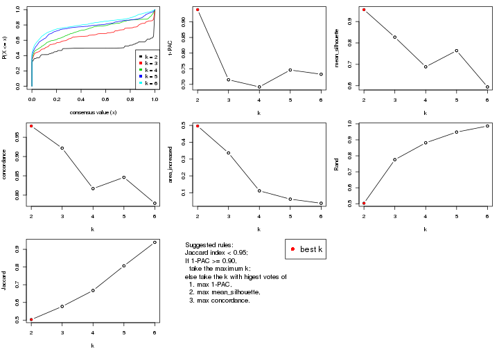
The numeric values for all these statistics can be obtained by get_stats().
get_stats(res)
#>   k 1-PAC mean_silhouette concordance area_increased  Rand Jaccard
#> 2 2 0.939           0.956       0.979         0.4965 0.503   0.503
#> 3 3 0.715           0.827       0.922         0.3365 0.776   0.577
#> 4 4 0.692           0.688       0.817         0.1116 0.882   0.667
#> 5 5 0.746           0.764       0.846         0.0620 0.949   0.807
#> 6 6 0.732           0.594       0.779         0.0377 0.987   0.940
suggest_best_k() suggests the best \(k\) based on these statistics. The rules are as follows:
suggest_best_k(res)
#> [1] 2
Following shows the table of the partitions (You need to click the show/hide
code output link to see it). The membership matrix (columns with name p*)
is inferred by
clue::cl_consensus()
function with the SE method. Basically the value in the membership matrix
represents the probability to belong to a certain group. The finall class
label for an item is determined with the group with highest probability it
belongs to.
In get_classes() function, the entropy is calculated from the membership
matrix and the silhouette score is calculated from the consensus matrix.
cbind(get_classes(res, k = 2), get_membership(res, k = 2))
#>           class entropy silhouette    p1    p2
#> SRR837437     2  0.0000      0.982 0.000 1.000
#> SRR837438     1  0.0000      0.972 1.000 0.000
#> SRR837439     2  0.0000      0.982 0.000 1.000
#> SRR837440     2  0.0000      0.982 0.000 1.000
#> SRR837441     2  0.0000      0.982 0.000 1.000
#> SRR837442     2  0.0000      0.982 0.000 1.000
#> SRR837443     2  0.0000      0.982 0.000 1.000
#> SRR837444     1  0.3584      0.917 0.932 0.068
#> SRR837445     2  0.6148      0.822 0.152 0.848
#> SRR837446     2  0.0000      0.982 0.000 1.000
#> SRR837447     1  0.0000      0.972 1.000 0.000
#> SRR837448     1  0.0000      0.972 1.000 0.000
#> SRR837449     1  0.0000      0.972 1.000 0.000
#> SRR837450     1  0.0000      0.972 1.000 0.000
#> SRR837451     2  0.0000      0.982 0.000 1.000
#> SRR837452     2  0.0000      0.982 0.000 1.000
#> SRR837453     2  0.0000      0.982 0.000 1.000
#> SRR837454     2  0.0000      0.982 0.000 1.000
#> SRR837455     1  0.0000      0.972 1.000 0.000
#> SRR837456     1  0.0000      0.972 1.000 0.000
#> SRR837457     2  0.0000      0.982 0.000 1.000
#> SRR837458     1  0.0000      0.972 1.000 0.000
#> SRR837459     2  0.0000      0.982 0.000 1.000
#> SRR837460     2  0.0000      0.982 0.000 1.000
#> SRR837461     2  0.0000      0.982 0.000 1.000
#> SRR837462     1  0.0000      0.972 1.000 0.000
#> SRR837463     1  0.0376      0.969 0.996 0.004
#> SRR837464     2  0.0938      0.973 0.012 0.988
#> SRR837465     1  0.1184      0.961 0.984 0.016
#> SRR837466     1  0.0000      0.972 1.000 0.000
#> SRR837467     2  0.0000      0.982 0.000 1.000
#> SRR837468     1  0.0000      0.972 1.000 0.000
#> SRR837469     1  0.0000      0.972 1.000 0.000
#> SRR837470     1  0.0000      0.972 1.000 0.000
#> SRR837471     2  0.0000      0.982 0.000 1.000
#> SRR837472     2  0.0000      0.982 0.000 1.000
#> SRR837473     1  0.3584      0.918 0.932 0.068
#> SRR837474     2  0.0000      0.982 0.000 1.000
#> SRR837475     2  0.0000      0.982 0.000 1.000
#> SRR837476     2  0.0000      0.982 0.000 1.000
#> SRR837477     1  0.6801      0.788 0.820 0.180
#> SRR837478     2  0.0000      0.982 0.000 1.000
#> SRR837479     2  0.0672      0.976 0.008 0.992
#> SRR837480     2  0.0000      0.982 0.000 1.000
#> SRR837481     2  0.3879      0.914 0.076 0.924
#> SRR837482     1  0.0000      0.972 1.000 0.000
#> SRR837483     1  0.0000      0.972 1.000 0.000
#> SRR837484     2  0.0000      0.982 0.000 1.000
#> SRR837485     2  0.0000      0.982 0.000 1.000
#> SRR837486     1  0.8081      0.681 0.752 0.248
#> SRR837487     2  0.0000      0.982 0.000 1.000
#> SRR837488     2  0.0000      0.982 0.000 1.000
#> SRR837489     2  0.0000      0.982 0.000 1.000
#> SRR837490     2  0.0000      0.982 0.000 1.000
#> SRR837491     2  0.5737      0.841 0.136 0.864
#> SRR837492     1  0.7453      0.747 0.788 0.212
#> SRR837493     1  0.0000      0.972 1.000 0.000
#> SRR837494     2  0.0000      0.982 0.000 1.000
#> SRR837495     2  0.8144      0.665 0.252 0.748
#> SRR837496     1  0.0000      0.972 1.000 0.000
#> SRR837497     1  0.0000      0.972 1.000 0.000
#> SRR837498     1  0.0000      0.972 1.000 0.000
#> SRR837499     1  0.0000      0.972 1.000 0.000
#> SRR837500     1  0.0000      0.972 1.000 0.000
#> SRR837501     2  0.2236      0.953 0.036 0.964
#> SRR837502     1  0.0000      0.972 1.000 0.000
#> SRR837503     1  0.0000      0.972 1.000 0.000
#> SRR837504     2  0.0000      0.982 0.000 1.000
#> SRR837505     2  0.0000      0.982 0.000 1.000
#> SRR837506     2  0.0000      0.982 0.000 1.000
cbind(get_classes(res, k = 3), get_membership(res, k = 3))
#>           class entropy silhouette    p1    p2    p3
#> SRR837437     2  0.2356     0.8928 0.000 0.928 0.072
#> SRR837438     1  0.4291     0.7388 0.820 0.000 0.180
#> SRR837439     2  0.3412     0.8418 0.000 0.876 0.124
#> SRR837440     3  0.5397     0.6515 0.000 0.280 0.720
#> SRR837441     2  0.3619     0.8275 0.000 0.864 0.136
#> SRR837442     2  0.0000     0.9441 0.000 1.000 0.000
#> SRR837443     3  0.5016     0.7043 0.000 0.240 0.760
#> SRR837444     3  0.5956     0.4758 0.324 0.004 0.672
#> SRR837445     2  0.3695     0.8400 0.108 0.880 0.012
#> SRR837446     3  0.1163     0.8472 0.000 0.028 0.972
#> SRR837447     1  0.0000     0.9134 1.000 0.000 0.000
#> SRR837448     1  0.0000     0.9134 1.000 0.000 0.000
#> SRR837449     1  0.0000     0.9134 1.000 0.000 0.000
#> SRR837450     1  0.0000     0.9134 1.000 0.000 0.000
#> SRR837451     2  0.0000     0.9441 0.000 1.000 0.000
#> SRR837452     2  0.0000     0.9441 0.000 1.000 0.000
#> SRR837453     2  0.0000     0.9441 0.000 1.000 0.000
#> SRR837454     2  0.0000     0.9441 0.000 1.000 0.000
#> SRR837455     1  0.0000     0.9134 1.000 0.000 0.000
#> SRR837456     1  0.0000     0.9134 1.000 0.000 0.000
#> SRR837457     2  0.0000     0.9441 0.000 1.000 0.000
#> SRR837458     1  0.0000     0.9134 1.000 0.000 0.000
#> SRR837459     2  0.0000     0.9441 0.000 1.000 0.000
#> SRR837460     2  0.0000     0.9441 0.000 1.000 0.000
#> SRR837461     3  0.5497     0.6331 0.000 0.292 0.708
#> SRR837462     1  0.6295     0.0731 0.528 0.000 0.472
#> SRR837463     3  0.7059     0.0795 0.460 0.020 0.520
#> SRR837464     3  0.2356     0.8369 0.000 0.072 0.928
#> SRR837465     1  0.2845     0.8520 0.920 0.068 0.012
#> SRR837466     1  0.0000     0.9134 1.000 0.000 0.000
#> SRR837467     2  0.0892     0.9334 0.000 0.980 0.020
#> SRR837468     3  0.0747     0.8428 0.016 0.000 0.984
#> SRR837469     1  0.0000     0.9134 1.000 0.000 0.000
#> SRR837470     1  0.0000     0.9134 1.000 0.000 0.000
#> SRR837471     2  0.0000     0.9441 0.000 1.000 0.000
#> SRR837472     2  0.0000     0.9441 0.000 1.000 0.000
#> SRR837473     1  0.3686     0.7854 0.860 0.140 0.000
#> SRR837474     2  0.0000     0.9441 0.000 1.000 0.000
#> SRR837475     2  0.0000     0.9441 0.000 1.000 0.000
#> SRR837476     2  0.0000     0.9441 0.000 1.000 0.000
#> SRR837477     1  0.8527     0.4539 0.612 0.196 0.192
#> SRR837478     2  0.5058     0.6698 0.000 0.756 0.244
#> SRR837479     3  0.0424     0.8481 0.000 0.008 0.992
#> SRR837480     2  0.5733     0.5254 0.000 0.676 0.324
#> SRR837481     3  0.0424     0.8481 0.000 0.008 0.992
#> SRR837482     3  0.2165     0.8183 0.064 0.000 0.936
#> SRR837483     1  0.0000     0.9134 1.000 0.000 0.000
#> SRR837484     3  0.5560     0.5789 0.000 0.300 0.700
#> SRR837485     3  0.3619     0.7831 0.000 0.136 0.864
#> SRR837486     3  0.0000     0.8463 0.000 0.000 1.000
#> SRR837487     2  0.0000     0.9441 0.000 1.000 0.000
#> SRR837488     2  0.0000     0.9441 0.000 1.000 0.000
#> SRR837489     2  0.0000     0.9441 0.000 1.000 0.000
#> SRR837490     2  0.0000     0.9441 0.000 1.000 0.000
#> SRR837491     2  0.1015     0.9329 0.012 0.980 0.008
#> SRR837492     1  0.6102     0.5318 0.672 0.320 0.008
#> SRR837493     1  0.5244     0.6440 0.756 0.004 0.240
#> SRR837494     2  0.2066     0.9036 0.000 0.940 0.060
#> SRR837495     2  0.3816     0.7991 0.148 0.852 0.000
#> SRR837496     1  0.0000     0.9134 1.000 0.000 0.000
#> SRR837497     1  0.0000     0.9134 1.000 0.000 0.000
#> SRR837498     1  0.0000     0.9134 1.000 0.000 0.000
#> SRR837499     1  0.0000     0.9134 1.000 0.000 0.000
#> SRR837500     1  0.0000     0.9134 1.000 0.000 0.000
#> SRR837501     3  0.0000     0.8463 0.000 0.000 1.000
#> SRR837502     1  0.0000     0.9134 1.000 0.000 0.000
#> SRR837503     1  0.0000     0.9134 1.000 0.000 0.000
#> SRR837504     3  0.3116     0.8211 0.000 0.108 0.892
#> SRR837505     3  0.0237     0.8475 0.000 0.004 0.996
#> SRR837506     3  0.0592     0.8481 0.000 0.012 0.988
cbind(get_classes(res, k = 4), get_membership(res, k = 4))
#>           class entropy silhouette    p1    p2    p3    p4
#> SRR837437     2  0.4776     0.5782 0.000 0.732 0.024 0.244
#> SRR837438     4  0.5417     0.5904 0.284 0.000 0.040 0.676
#> SRR837439     4  0.5024     0.4031 0.000 0.360 0.008 0.632
#> SRR837440     4  0.6346     0.5465 0.000 0.116 0.244 0.640
#> SRR837441     4  0.5313     0.3653 0.000 0.376 0.016 0.608
#> SRR837442     2  0.1004     0.8422 0.000 0.972 0.004 0.024
#> SRR837443     4  0.6118     0.5566 0.000 0.120 0.208 0.672
#> SRR837444     4  0.5470     0.4363 0.100 0.000 0.168 0.732
#> SRR837445     2  0.8113     0.2857 0.052 0.476 0.116 0.356
#> SRR837446     3  0.3672     0.6634 0.000 0.012 0.824 0.164
#> SRR837447     1  0.0000     0.9029 1.000 0.000 0.000 0.000
#> SRR837448     1  0.1389     0.8899 0.952 0.000 0.000 0.048
#> SRR837449     1  0.0000     0.9029 1.000 0.000 0.000 0.000
#> SRR837450     1  0.1389     0.8899 0.952 0.000 0.000 0.048
#> SRR837451     2  0.0188     0.8580 0.000 0.996 0.004 0.000
#> SRR837452     2  0.1004     0.8513 0.000 0.972 0.004 0.024
#> SRR837453     2  0.0188     0.8580 0.000 0.996 0.004 0.000
#> SRR837454     2  0.0524     0.8566 0.000 0.988 0.004 0.008
#> SRR837455     1  0.0000     0.9029 1.000 0.000 0.000 0.000
#> SRR837456     1  0.0000     0.9029 1.000 0.000 0.000 0.000
#> SRR837457     2  0.0188     0.8580 0.000 0.996 0.004 0.000
#> SRR837458     1  0.0000     0.9029 1.000 0.000 0.000 0.000
#> SRR837459     2  0.0188     0.8580 0.000 0.996 0.004 0.000
#> SRR837460     2  0.0188     0.8580 0.000 0.996 0.004 0.000
#> SRR837461     4  0.6120     0.5192 0.000 0.076 0.296 0.628
#> SRR837462     4  0.7585     0.4406 0.304 0.000 0.224 0.472
#> SRR837463     4  0.6039     0.5973 0.128 0.000 0.188 0.684
#> SRR837464     4  0.5093     0.4623 0.000 0.012 0.348 0.640
#> SRR837465     4  0.5167     0.1890 0.488 0.004 0.000 0.508
#> SRR837466     1  0.1389     0.8899 0.952 0.000 0.000 0.048
#> SRR837467     2  0.3982     0.6383 0.000 0.776 0.004 0.220
#> SRR837468     3  0.3945     0.6022 0.004 0.000 0.780 0.216
#> SRR837469     1  0.0469     0.8972 0.988 0.000 0.000 0.012
#> SRR837470     1  0.0469     0.8972 0.988 0.000 0.000 0.012
#> SRR837471     2  0.0817     0.8508 0.000 0.976 0.000 0.024
#> SRR837472     2  0.0817     0.8508 0.000 0.976 0.000 0.024
#> SRR837473     1  0.5670     0.6383 0.720 0.152 0.000 0.128
#> SRR837474     2  0.0817     0.8508 0.000 0.976 0.000 0.024
#> SRR837475     2  0.0817     0.8508 0.000 0.976 0.000 0.024
#> SRR837476     2  0.0657     0.8525 0.000 0.984 0.004 0.012
#> SRR837477     1  0.9153     0.0735 0.380 0.076 0.244 0.300
#> SRR837478     2  0.7721     0.0610 0.000 0.440 0.312 0.248
#> SRR837479     3  0.3074     0.6674 0.000 0.000 0.848 0.152
#> SRR837480     3  0.7618     0.2937 0.000 0.284 0.472 0.244
#> SRR837481     3  0.2973     0.6714 0.000 0.000 0.856 0.144
#> SRR837482     3  0.2919     0.6853 0.044 0.000 0.896 0.060
#> SRR837483     1  0.0779     0.9002 0.980 0.000 0.004 0.016
#> SRR837484     3  0.4585     0.4517 0.000 0.332 0.668 0.000
#> SRR837485     3  0.3688     0.6015 0.000 0.208 0.792 0.000
#> SRR837486     3  0.1716     0.7049 0.000 0.000 0.936 0.064
#> SRR837487     2  0.0188     0.8580 0.000 0.996 0.004 0.000
#> SRR837488     2  0.0188     0.8580 0.000 0.996 0.004 0.000
#> SRR837489     2  0.0000     0.8572 0.000 1.000 0.000 0.000
#> SRR837490     2  0.0188     0.8580 0.000 0.996 0.004 0.000
#> SRR837491     2  0.5331     0.4187 0.024 0.644 0.000 0.332
#> SRR837492     1  0.8538     0.2751 0.464 0.252 0.044 0.240
#> SRR837493     4  0.5663     0.5994 0.264 0.000 0.060 0.676
#> SRR837494     2  0.4453     0.5921 0.000 0.744 0.012 0.244
#> SRR837495     2  0.8274     0.3210 0.076 0.508 0.112 0.304
#> SRR837496     1  0.1474     0.8879 0.948 0.000 0.000 0.052
#> SRR837497     1  0.0000     0.9029 1.000 0.000 0.000 0.000
#> SRR837498     1  0.0469     0.8972 0.988 0.000 0.000 0.012
#> SRR837499     1  0.0000     0.9029 1.000 0.000 0.000 0.000
#> SRR837500     1  0.0817     0.8991 0.976 0.000 0.000 0.024
#> SRR837501     3  0.3444     0.6304 0.000 0.000 0.816 0.184
#> SRR837502     1  0.0336     0.9023 0.992 0.000 0.000 0.008
#> SRR837503     1  0.1302     0.8922 0.956 0.000 0.000 0.044
#> SRR837504     3  0.5512     0.5755 0.000 0.100 0.728 0.172
#> SRR837505     3  0.3157     0.6665 0.000 0.004 0.852 0.144
#> SRR837506     3  0.2662     0.7012 0.000 0.016 0.900 0.084
cbind(get_classes(res, k = 5), get_membership(res, k = 5))
#>           class entropy silhouette    p1    p2    p3    p4    p5
#> SRR837437     2  0.4674     0.5690 0.000 0.676 0.024 0.292 0.008
#> SRR837438     4  0.3693     0.6954 0.124 0.000 0.008 0.824 0.044
#> SRR837439     4  0.3587     0.6605 0.000 0.140 0.024 0.824 0.012
#> SRR837440     4  0.3809     0.6939 0.000 0.044 0.116 0.824 0.016
#> SRR837441     4  0.3961     0.6329 0.000 0.168 0.028 0.792 0.012
#> SRR837442     2  0.1924     0.8491 0.000 0.924 0.004 0.064 0.008
#> SRR837443     4  0.3948     0.6946 0.000 0.056 0.096 0.824 0.024
#> SRR837444     4  0.5462     0.5664 0.024 0.000 0.084 0.688 0.204
#> SRR837445     5  0.4045     0.7070 0.000 0.052 0.020 0.116 0.812
#> SRR837446     3  0.4037     0.6465 0.000 0.004 0.752 0.020 0.224
#> SRR837447     1  0.0000     0.9249 1.000 0.000 0.000 0.000 0.000
#> SRR837448     1  0.1830     0.9080 0.924 0.000 0.000 0.008 0.068
#> SRR837449     1  0.0290     0.9244 0.992 0.000 0.000 0.008 0.000
#> SRR837450     1  0.1830     0.9080 0.924 0.000 0.000 0.008 0.068
#> SRR837451     2  0.0000     0.8881 0.000 1.000 0.000 0.000 0.000
#> SRR837452     2  0.0955     0.8760 0.000 0.968 0.000 0.004 0.028
#> SRR837453     2  0.0000     0.8881 0.000 1.000 0.000 0.000 0.000
#> SRR837454     2  0.0162     0.8874 0.000 0.996 0.000 0.000 0.004
#> SRR837455     1  0.0162     0.9246 0.996 0.000 0.000 0.004 0.000
#> SRR837456     1  0.0162     0.9246 0.996 0.000 0.000 0.004 0.000
#> SRR837457     2  0.0000     0.8881 0.000 1.000 0.000 0.000 0.000
#> SRR837458     1  0.0162     0.9255 0.996 0.000 0.000 0.000 0.004
#> SRR837459     2  0.0000     0.8881 0.000 1.000 0.000 0.000 0.000
#> SRR837460     2  0.0000     0.8881 0.000 1.000 0.000 0.000 0.000
#> SRR837461     4  0.4985     0.6769 0.000 0.044 0.152 0.748 0.056
#> SRR837462     4  0.7600     0.4331 0.288 0.000 0.144 0.468 0.100
#> SRR837463     4  0.5262     0.6866 0.088 0.000 0.068 0.744 0.100
#> SRR837464     4  0.4581     0.6309 0.000 0.000 0.196 0.732 0.072
#> SRR837465     4  0.5666     0.5030 0.296 0.000 0.004 0.604 0.096
#> SRR837466     1  0.1830     0.9080 0.924 0.000 0.000 0.008 0.068
#> SRR837467     2  0.3937     0.6549 0.000 0.736 0.004 0.252 0.008
#> SRR837468     3  0.5229     0.6323 0.016 0.000 0.708 0.184 0.092
#> SRR837469     1  0.1836     0.8869 0.932 0.000 0.000 0.036 0.032
#> SRR837470     1  0.1493     0.8994 0.948 0.000 0.000 0.028 0.024
#> SRR837471     2  0.2361     0.8299 0.000 0.892 0.000 0.012 0.096
#> SRR837472     2  0.2130     0.8439 0.000 0.908 0.000 0.012 0.080
#> SRR837473     1  0.6240     0.2441 0.524 0.092 0.000 0.020 0.364
#> SRR837474     2  0.1894     0.8520 0.000 0.920 0.000 0.008 0.072
#> SRR837475     2  0.2077     0.8401 0.000 0.908 0.000 0.008 0.084
#> SRR837476     2  0.0566     0.8858 0.000 0.984 0.000 0.012 0.004
#> SRR837477     5  0.3770     0.7343 0.040 0.024 0.104 0.000 0.832
#> SRR837478     5  0.5236     0.7004 0.000 0.164 0.152 0.000 0.684
#> SRR837479     3  0.3010     0.7060 0.000 0.000 0.824 0.004 0.172
#> SRR837480     5  0.5508     0.6226 0.000 0.120 0.244 0.000 0.636
#> SRR837481     3  0.2648     0.7197 0.000 0.000 0.848 0.000 0.152
#> SRR837482     3  0.4236     0.7297 0.044 0.000 0.812 0.056 0.088
#> SRR837483     1  0.1492     0.9189 0.948 0.000 0.004 0.008 0.040
#> SRR837484     3  0.3797     0.6145 0.000 0.232 0.756 0.004 0.008
#> SRR837485     3  0.2886     0.7387 0.000 0.116 0.864 0.004 0.016
#> SRR837486     3  0.0898     0.7825 0.000 0.000 0.972 0.008 0.020
#> SRR837487     2  0.0000     0.8881 0.000 1.000 0.000 0.000 0.000
#> SRR837488     2  0.0000     0.8881 0.000 1.000 0.000 0.000 0.000
#> SRR837489     2  0.0451     0.8869 0.000 0.988 0.000 0.004 0.008
#> SRR837490     2  0.0324     0.8872 0.000 0.992 0.000 0.004 0.004
#> SRR837491     2  0.6329     0.0584 0.008 0.464 0.012 0.432 0.084
#> SRR837492     5  0.4451     0.5705 0.224 0.024 0.000 0.016 0.736
#> SRR837493     4  0.3812     0.6945 0.128 0.000 0.008 0.816 0.048
#> SRR837494     2  0.4669     0.5453 0.000 0.664 0.020 0.308 0.008
#> SRR837495     5  0.3287     0.7510 0.008 0.124 0.008 0.012 0.848
#> SRR837496     1  0.2563     0.8767 0.872 0.000 0.000 0.008 0.120
#> SRR837497     1  0.0798     0.9262 0.976 0.000 0.000 0.008 0.016
#> SRR837498     1  0.1403     0.9038 0.952 0.000 0.000 0.024 0.024
#> SRR837499     1  0.0579     0.9247 0.984 0.000 0.000 0.008 0.008
#> SRR837500     1  0.2331     0.8949 0.900 0.000 0.000 0.020 0.080
#> SRR837501     3  0.3432     0.7362 0.000 0.000 0.828 0.132 0.040
#> SRR837502     1  0.1626     0.9172 0.940 0.000 0.000 0.016 0.044
#> SRR837503     1  0.2189     0.9032 0.904 0.000 0.000 0.012 0.084
#> SRR837504     3  0.5429     0.6362 0.000 0.124 0.696 0.164 0.016
#> SRR837505     3  0.2789     0.7707 0.000 0.008 0.880 0.092 0.020
#> SRR837506     3  0.1978     0.7862 0.000 0.024 0.932 0.032 0.012
cbind(get_classes(res, k = 6), get_membership(res, k = 6))
#>           class entropy silhouette    p1    p2    p3    p4    p5    p6
#> SRR837437     2  0.6327   -0.17377 0.000 0.460 0.020 0.236 0.000 0.284
#> SRR837438     4  0.2255    0.30692 0.088 0.000 0.000 0.892 0.004 0.016
#> SRR837439     4  0.5002    0.01034 0.000 0.072 0.012 0.624 0.000 0.292
#> SRR837440     4  0.5055   -0.00998 0.000 0.024 0.040 0.572 0.000 0.364
#> SRR837441     4  0.5291   -0.01722 0.000 0.080 0.020 0.600 0.000 0.300
#> SRR837442     2  0.3424    0.66922 0.000 0.796 0.004 0.032 0.000 0.168
#> SRR837443     4  0.4942    0.03243 0.000 0.036 0.028 0.612 0.000 0.324
#> SRR837444     4  0.5966    0.18610 0.016 0.000 0.040 0.628 0.172 0.144
#> SRR837445     5  0.3406    0.73236 0.000 0.020 0.004 0.080 0.840 0.056
#> SRR837446     3  0.4784    0.49204 0.000 0.000 0.660 0.028 0.272 0.040
#> SRR837447     1  0.0622    0.87832 0.980 0.000 0.000 0.008 0.000 0.012
#> SRR837448     1  0.2279    0.86536 0.900 0.000 0.000 0.004 0.048 0.048
#> SRR837449     1  0.1088    0.87886 0.960 0.000 0.000 0.024 0.000 0.016
#> SRR837450     1  0.2408    0.86293 0.892 0.000 0.000 0.004 0.052 0.052
#> SRR837451     2  0.0000    0.84411 0.000 1.000 0.000 0.000 0.000 0.000
#> SRR837452     2  0.0820    0.83676 0.000 0.972 0.000 0.000 0.016 0.012
#> SRR837453     2  0.0000    0.84411 0.000 1.000 0.000 0.000 0.000 0.000
#> SRR837454     2  0.0000    0.84411 0.000 1.000 0.000 0.000 0.000 0.000
#> SRR837455     1  0.0806    0.87947 0.972 0.000 0.000 0.020 0.000 0.008
#> SRR837456     1  0.0909    0.87927 0.968 0.000 0.000 0.020 0.000 0.012
#> SRR837457     2  0.0000    0.84411 0.000 1.000 0.000 0.000 0.000 0.000
#> SRR837458     1  0.0405    0.88071 0.988 0.000 0.000 0.004 0.000 0.008
#> SRR837459     2  0.0000    0.84411 0.000 1.000 0.000 0.000 0.000 0.000
#> SRR837460     2  0.0000    0.84411 0.000 1.000 0.000 0.000 0.000 0.000
#> SRR837461     6  0.5410   -0.24622 0.000 0.020 0.068 0.396 0.000 0.516
#> SRR837462     4  0.6845    0.17324 0.184 0.000 0.076 0.448 0.000 0.292
#> SRR837463     4  0.4985    0.21047 0.036 0.000 0.056 0.668 0.000 0.240
#> SRR837464     4  0.5448    0.03537 0.000 0.000 0.132 0.516 0.000 0.352
#> SRR837465     4  0.5789    0.19737 0.216 0.000 0.004 0.588 0.016 0.176
#> SRR837466     1  0.2146    0.86699 0.908 0.000 0.000 0.004 0.044 0.044
#> SRR837467     2  0.5564    0.20114 0.000 0.580 0.008 0.164 0.000 0.248
#> SRR837468     3  0.5813    0.43439 0.008 0.000 0.500 0.156 0.000 0.336
#> SRR837469     1  0.3160    0.79576 0.840 0.000 0.008 0.104 0.000 0.048
#> SRR837470     1  0.2350    0.83849 0.888 0.000 0.000 0.076 0.000 0.036
#> SRR837471     2  0.3032    0.76314 0.000 0.840 0.000 0.000 0.056 0.104
#> SRR837472     2  0.2812    0.77597 0.000 0.856 0.000 0.000 0.048 0.096
#> SRR837473     1  0.7572   -0.15086 0.336 0.068 0.004 0.020 0.336 0.236
#> SRR837474     2  0.2724    0.78157 0.000 0.864 0.000 0.000 0.052 0.084
#> SRR837475     2  0.3032    0.76237 0.000 0.840 0.000 0.000 0.056 0.104
#> SRR837476     2  0.0865    0.83761 0.000 0.964 0.000 0.000 0.000 0.036
#> SRR837477     5  0.2128    0.75687 0.008 0.004 0.064 0.004 0.912 0.008
#> SRR837478     5  0.4059    0.69906 0.000 0.100 0.148 0.000 0.752 0.000
#> SRR837479     3  0.3529    0.59048 0.000 0.000 0.764 0.000 0.208 0.028
#> SRR837480     5  0.4144    0.65584 0.000 0.072 0.200 0.000 0.728 0.000
#> SRR837481     3  0.2909    0.62286 0.000 0.000 0.828 0.004 0.156 0.012
#> SRR837482     3  0.4579    0.65204 0.032 0.000 0.776 0.044 0.048 0.100
#> SRR837483     1  0.2745    0.85668 0.884 0.000 0.040 0.004 0.020 0.052
#> SRR837484     3  0.3765    0.60796 0.000 0.164 0.780 0.008 0.000 0.048
#> SRR837485     3  0.2979    0.65912 0.000 0.116 0.840 0.000 0.000 0.044
#> SRR837486     3  0.1297    0.69691 0.000 0.000 0.948 0.000 0.012 0.040
#> SRR837487     2  0.0405    0.84151 0.000 0.988 0.008 0.000 0.000 0.004
#> SRR837488     2  0.0000    0.84411 0.000 1.000 0.000 0.000 0.000 0.000
#> SRR837489     2  0.1327    0.82422 0.000 0.936 0.000 0.000 0.000 0.064
#> SRR837490     2  0.1075    0.83116 0.000 0.952 0.000 0.000 0.000 0.048
#> SRR837491     6  0.7377    0.06748 0.012 0.252 0.000 0.324 0.072 0.340
#> SRR837492     5  0.4811    0.56258 0.120 0.000 0.004 0.004 0.692 0.180
#> SRR837493     4  0.3126    0.30801 0.104 0.000 0.004 0.844 0.004 0.044
#> SRR837494     2  0.5981   -0.01099 0.000 0.512 0.012 0.196 0.000 0.280
#> SRR837495     5  0.2954    0.74766 0.000 0.044 0.000 0.028 0.868 0.060
#> SRR837496     1  0.3112    0.83788 0.840 0.000 0.000 0.004 0.104 0.052
#> SRR837497     1  0.1332    0.88110 0.952 0.000 0.000 0.012 0.008 0.028
#> SRR837498     1  0.2221    0.84528 0.896 0.000 0.000 0.072 0.000 0.032
#> SRR837499     1  0.1829    0.87345 0.928 0.000 0.000 0.036 0.008 0.028
#> SRR837500     1  0.4467    0.75103 0.756 0.000 0.000 0.048 0.064 0.132
#> SRR837501     3  0.4697    0.57878 0.000 0.000 0.612 0.064 0.000 0.324
#> SRR837502     1  0.3716    0.81277 0.816 0.000 0.000 0.044 0.044 0.096
#> SRR837503     1  0.2036    0.87454 0.916 0.000 0.000 0.008 0.048 0.028
#> SRR837504     3  0.6182    0.45161 0.000 0.068 0.528 0.096 0.000 0.308
#> SRR837505     3  0.3652    0.65595 0.000 0.000 0.720 0.016 0.000 0.264
#> SRR837506     3  0.3056    0.69778 0.000 0.008 0.804 0.000 0.004 0.184
Heatmaps for the consensus matrix. It visualizes the probability of two samples to be in a same group.
consensus_heatmap(res, k = 2)
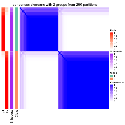
consensus_heatmap(res, k = 3)
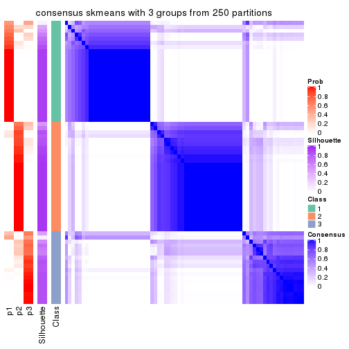
consensus_heatmap(res, k = 4)
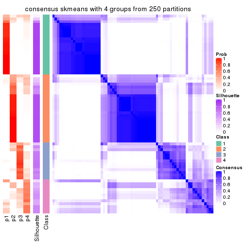
consensus_heatmap(res, k = 5)
consensus_heatmap(res, k = 6)
Heatmaps for the membership of samples in all partitions to see how consistent they are:
membership_heatmap(res, k = 2)
membership_heatmap(res, k = 3)
membership_heatmap(res, k = 4)
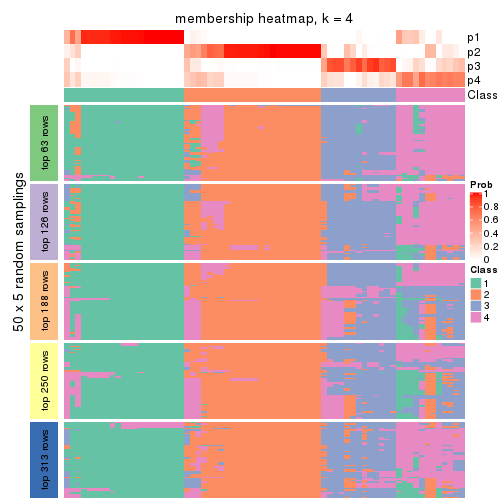
membership_heatmap(res, k = 5)
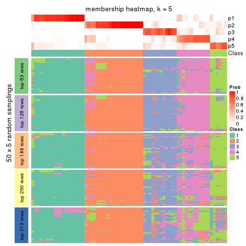
membership_heatmap(res, k = 6)
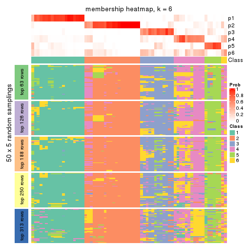
As soon as we have had the classes for columns, we can look for signatures which are significantly different between classes which can be candidate marks for certain classes. Following are the heatmaps for signatures.
Signature heatmaps where rows are scaled:
get_signatures(res, k = 2)
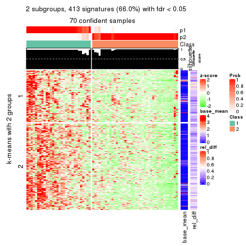
get_signatures(res, k = 3)
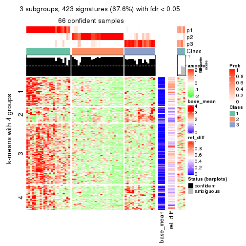
get_signatures(res, k = 4)
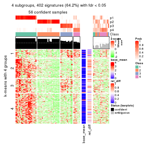
get_signatures(res, k = 5)
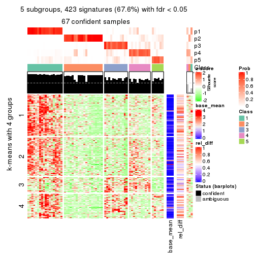
get_signatures(res, k = 6)

Signature heatmaps where rows are not scaled:
get_signatures(res, k = 2, scale_rows = FALSE)

get_signatures(res, k = 3, scale_rows = FALSE)
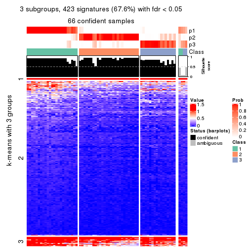
get_signatures(res, k = 4, scale_rows = FALSE)
get_signatures(res, k = 5, scale_rows = FALSE)
get_signatures(res, k = 6, scale_rows = FALSE)
Compare the overlap of signatures from different k:
compare_signatures(res)
get_signature() returns a data frame invisibly. TO get the list of signatures, the function
call should be assigned to a variable explicitly. In following code, if plot argument is set
to FALSE, no heatmap is plotted while only the differential analysis is performed.
# code only for demonstration
tb = get_signature(res, k = ..., plot = FALSE)
An example of the output of tb is:
#>   which_row         fdr    mean_1    mean_2 scaled_mean_1 scaled_mean_2 km
#> 1        38 0.042760348  8.373488  9.131774    -0.5533452     0.5164555  1
#> 2        40 0.018707592  7.106213  8.469186    -0.6173731     0.5762149  1
#> 3        55 0.019134737 10.221463 11.207825    -0.6159697     0.5749050  1
#> 4        59 0.006059896  5.921854  7.869574    -0.6899429     0.6439467  1
#> 5        60 0.018055526  8.928898 10.211722    -0.6204761     0.5791110  1
#> 6        98 0.009384629 15.714769 14.887706     0.6635654    -0.6193277  2
...
The columns in tb are:
which_row: row indices corresponding to the input matrix.fdr: FDR for the differential test. mean_x: The mean value in group x.scaled_mean_x: The mean value in group x after rows are scaled.km: Row groups if k-means clustering is applied to rows.UMAP plot which shows how samples are separated.
dimension_reduction(res, k = 2, method = "UMAP")
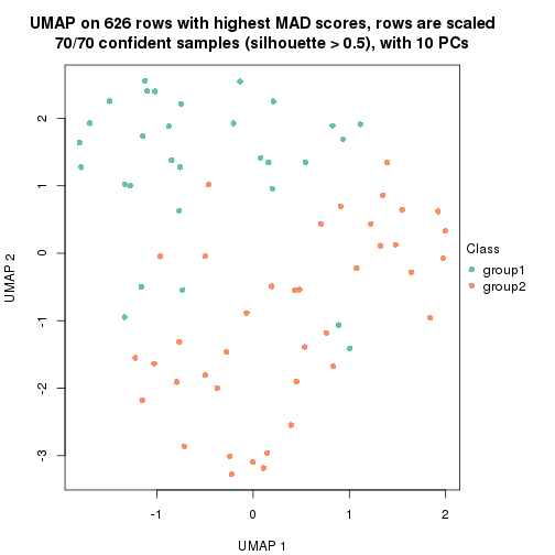
dimension_reduction(res, k = 3, method = "UMAP")
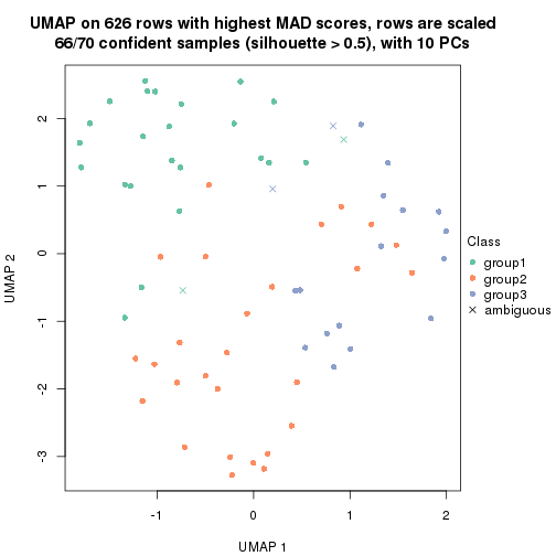
dimension_reduction(res, k = 4, method = "UMAP")
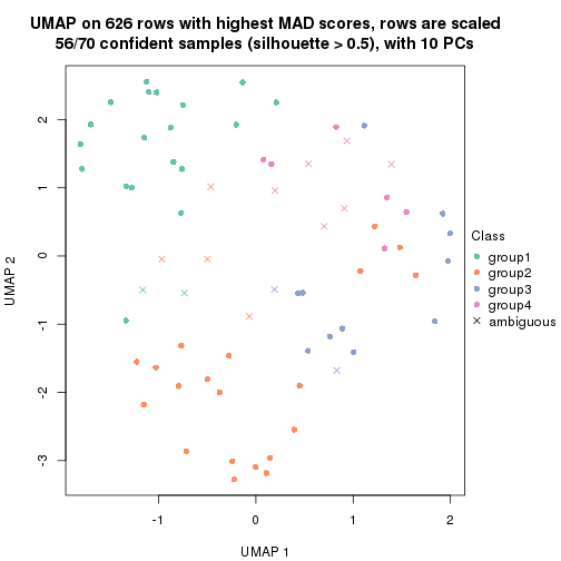
dimension_reduction(res, k = 5, method = "UMAP")
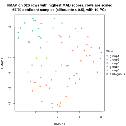
dimension_reduction(res, k = 6, method = "UMAP")
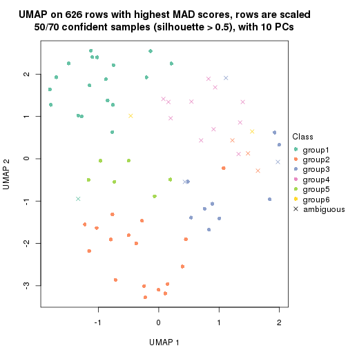
Following heatmap shows how subgroups are split when increasing k:
collect_classes(res)
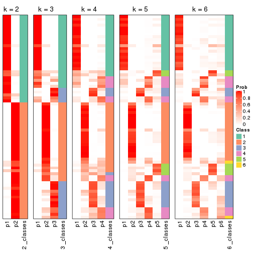
If matrix rows can be associated to genes, consider to use functional_enrichment(res,
...) to perform function enrichment for the signature genes. See this vignette for more detailed explanations.
The object with results only for a single top-value method and a single partition method can be extracted as:
res = res_list["MAD", "pam"]
# you can also extract it by
# res = res_list["MAD:pam"]
A summary of res and all the functions that can be applied to it:
res
#> A 'ConsensusPartition' object with k = 2, 3, 4, 5, 6.
#>   On a matrix with 626 rows and 70 columns.
#>   Top rows (63, 126, 188, 250, 313) are extracted by 'MAD' method.
#>   Subgroups are detected by 'pam' method.
#>   Performed in total 1250 partitions by row resampling.
#>   Best k for subgroups seems to be 2.
#>
#> Following methods can be applied to this 'ConsensusPartition' object:
#>  [1] "cola_report"             "collect_classes"         "collect_plots"
#>  [4] "collect_stats"           "colnames"                "compare_signatures"
#>  [7] "consensus_heatmap"       "dimension_reduction"     "functional_enrichment"
#> [10] "get_anno_col"            "get_anno"                "get_classes"
#> [13] "get_consensus"           "get_matrix"              "get_membership"
#> [16] "get_param"               "get_signatures"          "get_stats"
#> [19] "is_best_k"               "is_stable_k"             "membership_heatmap"
#> [22] "ncol"                    "nrow"                    "plot_ecdf"
#> [25] "rownames"                "select_partition_number" "show"
#> [28] "suggest_best_k"          "test_to_known_factors"
collect_plots() function collects all the plots made from res for all k (number of partitions)
into one single page to provide an easy and fast comparison between different k.
collect_plots(res)
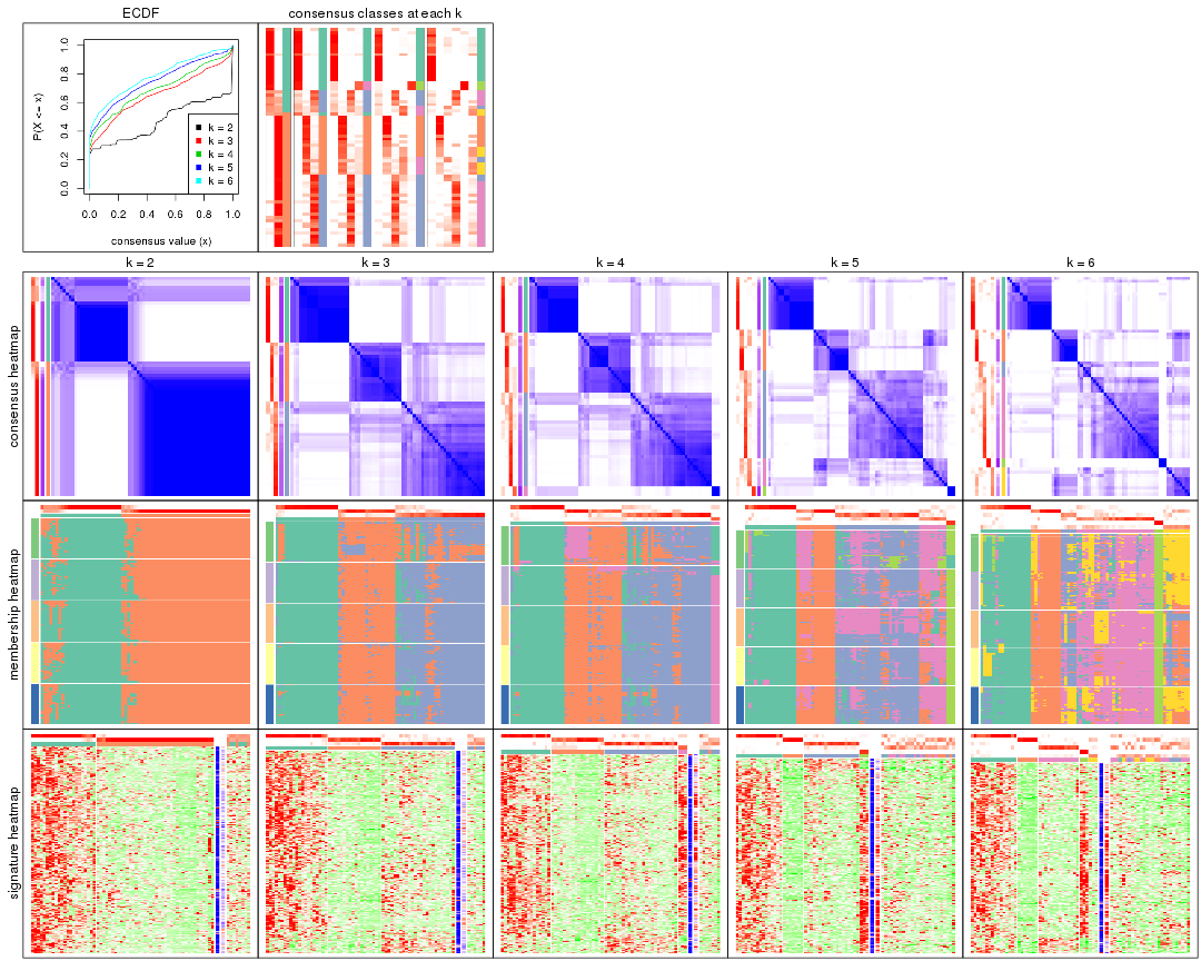
The plots are:
k and the heatmap of
predicted classes for each k.k.k.k.All the plots in panels can be made by individual functions and they are plotted later in this section.
select_partition_number() produces several plots showing different
statistics for choosing “optimized” k. There are following statistics:
k;k, the area increased is defined as \(A_k - A_{k-1}\).The detailed explanations of these statistics can be found in the cola vignette.
Generally speaking, lower PAC score, higher mean silhouette score or higher
concordance corresponds to better partition. Rand index and Jaccard index
measure how similar the current partition is compared to partition with k-1.
If they are too similar, we won't accept k is better than k-1.
select_partition_number(res)
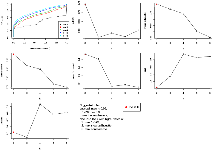
The numeric values for all these statistics can be obtained by get_stats().
get_stats(res)
#>   k 1-PAC mean_silhouette concordance area_increased  Rand Jaccard
#> 2 2 0.744           0.823       0.930         0.4694 0.519   0.519
#> 3 3 0.565           0.783       0.868         0.4067 0.669   0.443
#> 4 4 0.587           0.745       0.848         0.0592 0.978   0.934
#> 5 5 0.568           0.605       0.769         0.0785 0.929   0.781
#> 6 6 0.602           0.555       0.749         0.0456 0.949   0.811
suggest_best_k() suggests the best \(k\) based on these statistics. The rules are as follows:
suggest_best_k(res)
#> [1] 2
Following shows the table of the partitions (You need to click the show/hide
code output link to see it). The membership matrix (columns with name p*)
is inferred by
clue::cl_consensus()
function with the SE method. Basically the value in the membership matrix
represents the probability to belong to a certain group. The finall class
label for an item is determined with the group with highest probability it
belongs to.
In get_classes() function, the entropy is calculated from the membership
matrix and the silhouette score is calculated from the consensus matrix.
cbind(get_classes(res, k = 2), get_membership(res, k = 2))
#>           class entropy silhouette    p1    p2
#> SRR837437     2  0.0000     0.9501 0.000 1.000
#> SRR837438     1  0.3733     0.8358 0.928 0.072
#> SRR837439     2  0.0000     0.9501 0.000 1.000
#> SRR837440     2  0.0000     0.9501 0.000 1.000
#> SRR837441     2  0.0000     0.9501 0.000 1.000
#> SRR837442     2  0.0000     0.9501 0.000 1.000
#> SRR837443     2  0.0000     0.9501 0.000 1.000
#> SRR837444     1  0.9963     0.2375 0.536 0.464
#> SRR837445     2  0.8763     0.5269 0.296 0.704
#> SRR837446     2  0.0000     0.9501 0.000 1.000
#> SRR837447     1  0.0000     0.8757 1.000 0.000
#> SRR837448     1  0.0000     0.8757 1.000 0.000
#> SRR837449     1  0.0000     0.8757 1.000 0.000
#> SRR837450     1  0.0938     0.8698 0.988 0.012
#> SRR837451     2  0.0000     0.9501 0.000 1.000
#> SRR837452     2  0.0000     0.9501 0.000 1.000
#> SRR837453     2  0.0000     0.9501 0.000 1.000
#> SRR837454     2  0.0000     0.9501 0.000 1.000
#> SRR837455     1  0.0000     0.8757 1.000 0.000
#> SRR837456     1  0.0000     0.8757 1.000 0.000
#> SRR837457     2  0.0000     0.9501 0.000 1.000
#> SRR837458     1  0.0000     0.8757 1.000 0.000
#> SRR837459     2  0.0000     0.9501 0.000 1.000
#> SRR837460     2  0.0000     0.9501 0.000 1.000
#> SRR837461     2  0.0000     0.9501 0.000 1.000
#> SRR837462     1  0.6887     0.7445 0.816 0.184
#> SRR837463     1  0.9850     0.3432 0.572 0.428
#> SRR837464     2  0.0376     0.9468 0.004 0.996
#> SRR837465     1  0.9922     0.2915 0.552 0.448
#> SRR837466     1  0.0000     0.8757 1.000 0.000
#> SRR837467     2  0.0000     0.9501 0.000 1.000
#> SRR837468     2  0.9323     0.3927 0.348 0.652
#> SRR837469     1  0.0000     0.8757 1.000 0.000
#> SRR837470     1  0.0000     0.8757 1.000 0.000
#> SRR837471     2  0.0000     0.9501 0.000 1.000
#> SRR837472     2  0.0000     0.9501 0.000 1.000
#> SRR837473     1  0.6973     0.7381 0.812 0.188
#> SRR837474     2  0.0000     0.9501 0.000 1.000
#> SRR837475     2  0.0000     0.9501 0.000 1.000
#> SRR837476     2  0.0000     0.9501 0.000 1.000
#> SRR837477     1  0.9954     0.2484 0.540 0.460
#> SRR837478     2  0.0000     0.9501 0.000 1.000
#> SRR837479     2  0.0000     0.9501 0.000 1.000
#> SRR837480     2  0.0000     0.9501 0.000 1.000
#> SRR837481     2  0.0672     0.9432 0.008 0.992
#> SRR837482     2  0.9998    -0.1181 0.492 0.508
#> SRR837483     1  0.0000     0.8757 1.000 0.000
#> SRR837484     2  0.0000     0.9501 0.000 1.000
#> SRR837485     2  0.0000     0.9501 0.000 1.000
#> SRR837486     2  0.3879     0.8754 0.076 0.924
#> SRR837487     2  0.0000     0.9501 0.000 1.000
#> SRR837488     2  0.0000     0.9501 0.000 1.000
#> SRR837489     2  0.0000     0.9501 0.000 1.000
#> SRR837490     2  0.0000     0.9501 0.000 1.000
#> SRR837491     2  0.6048     0.7885 0.148 0.852
#> SRR837492     2  0.9954     0.0216 0.460 0.540
#> SRR837493     1  0.9087     0.5536 0.676 0.324
#> SRR837494     2  0.0000     0.9501 0.000 1.000
#> SRR837495     1  0.9963     0.2381 0.536 0.464
#> SRR837496     1  0.0000     0.8757 1.000 0.000
#> SRR837497     1  0.0000     0.8757 1.000 0.000
#> SRR837498     1  0.0000     0.8757 1.000 0.000
#> SRR837499     1  0.0000     0.8757 1.000 0.000
#> SRR837500     1  0.0000     0.8757 1.000 0.000
#> SRR837501     2  0.0672     0.9435 0.008 0.992
#> SRR837502     1  0.0000     0.8757 1.000 0.000
#> SRR837503     1  0.0000     0.8757 1.000 0.000
#> SRR837504     2  0.0000     0.9501 0.000 1.000
#> SRR837505     2  0.0000     0.9501 0.000 1.000
#> SRR837506     2  0.0000     0.9501 0.000 1.000
cbind(get_classes(res, k = 3), get_membership(res, k = 3))
#>           class entropy silhouette    p1    p2    p3
#> SRR837437     3  0.4121      0.732 0.000 0.168 0.832
#> SRR837438     1  0.4796      0.663 0.780 0.000 0.220
#> SRR837439     3  0.2625      0.777 0.000 0.084 0.916
#> SRR837440     3  0.1031      0.793 0.000 0.024 0.976
#> SRR837441     3  0.2165      0.785 0.000 0.064 0.936
#> SRR837442     3  0.5431      0.613 0.000 0.284 0.716
#> SRR837443     3  0.1411      0.792 0.000 0.036 0.964
#> SRR837444     3  0.4485      0.763 0.136 0.020 0.844
#> SRR837445     3  0.7265      0.692 0.128 0.160 0.712
#> SRR837446     3  0.0747      0.791 0.000 0.016 0.984
#> SRR837447     1  0.0475      0.954 0.992 0.004 0.004
#> SRR837448     1  0.0829      0.951 0.984 0.012 0.004
#> SRR837449     1  0.0000      0.956 1.000 0.000 0.000
#> SRR837450     1  0.0983      0.949 0.980 0.016 0.004
#> SRR837451     2  0.1289      0.882 0.000 0.968 0.032
#> SRR837452     2  0.2356      0.890 0.000 0.928 0.072
#> SRR837453     2  0.0747      0.883 0.000 0.984 0.016
#> SRR837454     2  0.0592      0.881 0.000 0.988 0.012
#> SRR837455     1  0.0000      0.956 1.000 0.000 0.000
#> SRR837456     1  0.0000      0.956 1.000 0.000 0.000
#> SRR837457     2  0.2625      0.854 0.000 0.916 0.084
#> SRR837458     1  0.0475      0.954 0.992 0.004 0.004
#> SRR837459     2  0.1411      0.881 0.000 0.964 0.036
#> SRR837460     2  0.1529      0.881 0.000 0.960 0.040
#> SRR837461     3  0.1643      0.792 0.000 0.044 0.956
#> SRR837462     3  0.5650      0.588 0.312 0.000 0.688
#> SRR837463     3  0.4293      0.746 0.164 0.004 0.832
#> SRR837464     3  0.0892      0.792 0.000 0.020 0.980
#> SRR837465     3  0.8137      0.632 0.220 0.140 0.640
#> SRR837466     1  0.0829      0.951 0.984 0.012 0.004
#> SRR837467     3  0.5529      0.574 0.000 0.296 0.704
#> SRR837468     3  0.0983      0.790 0.016 0.004 0.980
#> SRR837469     1  0.0475      0.954 0.992 0.004 0.004
#> SRR837470     1  0.0475      0.954 0.992 0.004 0.004
#> SRR837471     2  0.3425      0.877 0.004 0.884 0.112
#> SRR837472     2  0.2261      0.890 0.000 0.932 0.068
#> SRR837473     1  0.5473      0.747 0.808 0.140 0.052
#> SRR837474     2  0.4504      0.791 0.000 0.804 0.196
#> SRR837475     2  0.2066      0.889 0.000 0.940 0.060
#> SRR837476     2  0.3038      0.888 0.000 0.896 0.104
#> SRR837477     3  0.9154      0.310 0.384 0.148 0.468
#> SRR837478     2  0.3267      0.873 0.000 0.884 0.116
#> SRR837479     3  0.0892      0.792 0.000 0.020 0.980
#> SRR837480     2  0.6260      0.220 0.000 0.552 0.448
#> SRR837481     3  0.1163      0.792 0.000 0.028 0.972
#> SRR837482     3  0.5115      0.732 0.188 0.016 0.796
#> SRR837483     1  0.0000      0.956 1.000 0.000 0.000
#> SRR837484     3  0.5968      0.332 0.000 0.364 0.636
#> SRR837485     3  0.6154      0.188 0.000 0.408 0.592
#> SRR837486     3  0.1182      0.793 0.012 0.012 0.976
#> SRR837487     2  0.3038      0.885 0.000 0.896 0.104
#> SRR837488     2  0.0747      0.883 0.000 0.984 0.016
#> SRR837489     2  0.5327      0.663 0.000 0.728 0.272
#> SRR837490     2  0.2537      0.890 0.000 0.920 0.080
#> SRR837491     3  0.7670      0.669 0.152 0.164 0.684
#> SRR837492     1  0.7398      0.592 0.700 0.180 0.120
#> SRR837493     3  0.6169      0.522 0.360 0.004 0.636
#> SRR837494     2  0.5016      0.714 0.000 0.760 0.240
#> SRR837495     3  0.8930      0.497 0.316 0.148 0.536
#> SRR837496     1  0.0000      0.956 1.000 0.000 0.000
#> SRR837497     1  0.0000      0.956 1.000 0.000 0.000
#> SRR837498     1  0.0000      0.956 1.000 0.000 0.000
#> SRR837499     1  0.0000      0.956 1.000 0.000 0.000
#> SRR837500     1  0.0000      0.956 1.000 0.000 0.000
#> SRR837501     3  0.0237      0.790 0.000 0.004 0.996
#> SRR837502     1  0.0000      0.956 1.000 0.000 0.000
#> SRR837503     1  0.0000      0.956 1.000 0.000 0.000
#> SRR837504     3  0.1529      0.788 0.000 0.040 0.960
#> SRR837505     3  0.2066      0.777 0.000 0.060 0.940
#> SRR837506     3  0.5988      0.351 0.000 0.368 0.632
cbind(get_classes(res, k = 4), get_membership(res, k = 4))
#>           class entropy silhouette    p1    p2    p3    p4
#> SRR837437     3  0.4171      0.743 0.000 0.084 0.828 0.088
#> SRR837438     1  0.3942      0.520 0.764 0.000 0.236 0.000
#> SRR837439     3  0.2521      0.779 0.000 0.024 0.912 0.064
#> SRR837440     3  0.0336      0.786 0.000 0.008 0.992 0.000
#> SRR837441     3  0.1888      0.786 0.000 0.016 0.940 0.044
#> SRR837442     3  0.6284      0.594 0.000 0.164 0.664 0.172
#> SRR837443     3  0.1151      0.788 0.000 0.008 0.968 0.024
#> SRR837444     3  0.3598      0.752 0.124 0.000 0.848 0.028
#> SRR837445     3  0.6993      0.675 0.108 0.060 0.672 0.160
#> SRR837446     3  0.1211      0.782 0.000 0.000 0.960 0.040
#> SRR837447     1  0.0921      0.895 0.972 0.000 0.000 0.028
#> SRR837448     4  0.3837      1.000 0.224 0.000 0.000 0.776
#> SRR837449     1  0.0000      0.914 1.000 0.000 0.000 0.000
#> SRR837450     4  0.3837      1.000 0.224 0.000 0.000 0.776
#> SRR837451     2  0.0657      0.794 0.000 0.984 0.012 0.004
#> SRR837452     2  0.4244      0.819 0.000 0.800 0.032 0.168
#> SRR837453     2  0.0524      0.795 0.000 0.988 0.008 0.004
#> SRR837454     2  0.0188      0.793 0.000 0.996 0.000 0.004
#> SRR837455     1  0.0000      0.914 1.000 0.000 0.000 0.000
#> SRR837456     1  0.0000      0.914 1.000 0.000 0.000 0.000
#> SRR837457     2  0.1398      0.776 0.000 0.956 0.040 0.004
#> SRR837458     1  0.0707      0.902 0.980 0.000 0.000 0.020
#> SRR837459     2  0.0657      0.794 0.000 0.984 0.012 0.004
#> SRR837460     2  0.0657      0.794 0.000 0.984 0.012 0.004
#> SRR837461     3  0.1256      0.788 0.000 0.008 0.964 0.028
#> SRR837462     3  0.4382      0.573 0.296 0.000 0.704 0.000
#> SRR837463     3  0.3157      0.734 0.144 0.000 0.852 0.004
#> SRR837464     3  0.0336      0.786 0.000 0.008 0.992 0.000
#> SRR837465     3  0.7667      0.582 0.220 0.060 0.600 0.120
#> SRR837466     4  0.3837      1.000 0.224 0.000 0.000 0.776
#> SRR837467     3  0.5655      0.602 0.000 0.212 0.704 0.084
#> SRR837468     3  0.1209      0.778 0.004 0.000 0.964 0.032
#> SRR837469     1  0.0707      0.902 0.980 0.000 0.000 0.020
#> SRR837470     1  0.0707      0.902 0.980 0.000 0.000 0.020
#> SRR837471     2  0.5118      0.810 0.000 0.752 0.072 0.176
#> SRR837472     2  0.4149      0.818 0.000 0.804 0.028 0.168
#> SRR837473     1  0.5389      0.578 0.756 0.036 0.032 0.176
#> SRR837474     2  0.6198      0.741 0.000 0.672 0.152 0.176
#> SRR837475     2  0.3991      0.817 0.000 0.808 0.020 0.172
#> SRR837476     2  0.4937      0.820 0.000 0.764 0.064 0.172
#> SRR837477     3  0.8704      0.306 0.324 0.056 0.428 0.192
#> SRR837478     2  0.5160      0.802 0.000 0.748 0.072 0.180
#> SRR837479     3  0.1576      0.780 0.000 0.004 0.948 0.048
#> SRR837480     2  0.7213      0.155 0.000 0.452 0.408 0.140
#> SRR837481     3  0.1902      0.782 0.000 0.004 0.932 0.064
#> SRR837482     3  0.4635      0.717 0.160 0.020 0.796 0.024
#> SRR837483     1  0.0000      0.914 1.000 0.000 0.000 0.000
#> SRR837484     3  0.5478      0.367 0.000 0.344 0.628 0.028
#> SRR837485     3  0.5781      0.222 0.000 0.380 0.584 0.036
#> SRR837486     3  0.1585      0.786 0.004 0.004 0.952 0.040
#> SRR837487     2  0.5033      0.818 0.000 0.760 0.072 0.168
#> SRR837488     2  0.0524      0.797 0.000 0.988 0.008 0.004
#> SRR837489     2  0.6942      0.603 0.000 0.584 0.240 0.176
#> SRR837490     2  0.4088      0.826 0.000 0.820 0.040 0.140
#> SRR837491     3  0.7268      0.657 0.148 0.072 0.656 0.124
#> SRR837492     1  0.7032      0.442 0.664 0.072 0.080 0.184
#> SRR837493     3  0.4990      0.506 0.352 0.000 0.640 0.008
#> SRR837494     2  0.4360      0.669 0.000 0.744 0.248 0.008
#> SRR837495     3  0.8434      0.445 0.272 0.060 0.500 0.168
#> SRR837496     1  0.0000      0.914 1.000 0.000 0.000 0.000
#> SRR837497     1  0.0000      0.914 1.000 0.000 0.000 0.000
#> SRR837498     1  0.0000      0.914 1.000 0.000 0.000 0.000
#> SRR837499     1  0.0000      0.914 1.000 0.000 0.000 0.000
#> SRR837500     1  0.0000      0.914 1.000 0.000 0.000 0.000
#> SRR837501     3  0.0469      0.781 0.000 0.000 0.988 0.012
#> SRR837502     1  0.0000      0.914 1.000 0.000 0.000 0.000
#> SRR837503     1  0.0000      0.914 1.000 0.000 0.000 0.000
#> SRR837504     3  0.0804      0.785 0.000 0.012 0.980 0.008
#> SRR837505     3  0.2376      0.769 0.000 0.068 0.916 0.016
#> SRR837506     3  0.5510      0.319 0.000 0.376 0.600 0.024
cbind(get_classes(res, k = 5), get_membership(res, k = 5))
#>           class entropy silhouette    p1    p2    p3    p4    p5
#> SRR837437     3  0.3779     0.6770 0.000 0.056 0.816 0.124 0.004
#> SRR837438     1  0.3635     0.5802 0.748 0.000 0.248 0.000 0.004
#> SRR837439     3  0.2464     0.7042 0.000 0.012 0.892 0.092 0.004
#> SRR837440     3  0.1282     0.7212 0.000 0.000 0.952 0.044 0.004
#> SRR837441     3  0.2068     0.7082 0.000 0.000 0.904 0.092 0.004
#> SRR837442     3  0.5285     0.3558 0.000 0.060 0.584 0.356 0.000
#> SRR837443     3  0.1282     0.7189 0.000 0.000 0.952 0.044 0.004
#> SRR837444     3  0.3366     0.6993 0.116 0.000 0.844 0.032 0.008
#> SRR837445     3  0.5306     0.4400 0.072 0.000 0.612 0.316 0.000
#> SRR837446     3  0.2592     0.7102 0.000 0.000 0.892 0.052 0.056
#> SRR837447     1  0.2707     0.8076 0.860 0.000 0.000 0.008 0.132
#> SRR837448     5  0.1544     1.0000 0.068 0.000 0.000 0.000 0.932
#> SRR837449     1  0.0000     0.9223 1.000 0.000 0.000 0.000 0.000
#> SRR837450     5  0.1544     1.0000 0.068 0.000 0.000 0.000 0.932
#> SRR837451     2  0.0000     0.6846 0.000 1.000 0.000 0.000 0.000
#> SRR837452     2  0.4829    -0.0791 0.000 0.500 0.020 0.480 0.000
#> SRR837453     2  0.0000     0.6846 0.000 1.000 0.000 0.000 0.000
#> SRR837454     2  0.0609     0.6769 0.000 0.980 0.000 0.020 0.000
#> SRR837455     1  0.1041     0.9075 0.964 0.000 0.000 0.032 0.004
#> SRR837456     1  0.1041     0.9075 0.964 0.000 0.000 0.032 0.004
#> SRR837457     2  0.0000     0.6846 0.000 1.000 0.000 0.000 0.000
#> SRR837458     1  0.1836     0.8921 0.932 0.000 0.000 0.036 0.032
#> SRR837459     2  0.0000     0.6846 0.000 1.000 0.000 0.000 0.000
#> SRR837460     2  0.0000     0.6846 0.000 1.000 0.000 0.000 0.000
#> SRR837461     3  0.1430     0.7169 0.000 0.000 0.944 0.052 0.004
#> SRR837462     3  0.4360     0.5567 0.284 0.000 0.692 0.024 0.000
#> SRR837463     3  0.2929     0.6885 0.128 0.000 0.856 0.012 0.004
#> SRR837464     3  0.1043     0.7210 0.000 0.000 0.960 0.040 0.000
#> SRR837465     3  0.6201     0.3208 0.148 0.000 0.544 0.304 0.004
#> SRR837466     5  0.1544     1.0000 0.068 0.000 0.000 0.000 0.932
#> SRR837467     3  0.5118     0.5649 0.000 0.132 0.708 0.156 0.004
#> SRR837468     3  0.2074     0.7165 0.000 0.000 0.920 0.044 0.036
#> SRR837469     1  0.0955     0.9089 0.968 0.000 0.000 0.004 0.028
#> SRR837470     1  0.0955     0.9089 0.968 0.000 0.000 0.004 0.028
#> SRR837471     4  0.5359     0.1449 0.000 0.412 0.056 0.532 0.000
#> SRR837472     2  0.4818     0.0234 0.000 0.520 0.020 0.460 0.000
#> SRR837473     1  0.4610     0.2341 0.596 0.000 0.016 0.388 0.000
#> SRR837474     4  0.5894     0.2928 0.000 0.356 0.112 0.532 0.000
#> SRR837475     2  0.4430     0.2953 0.000 0.628 0.012 0.360 0.000
#> SRR837476     2  0.5088     0.0772 0.000 0.528 0.036 0.436 0.000
#> SRR837477     4  0.5338     0.4959 0.128 0.000 0.088 0.732 0.052
#> SRR837478     4  0.5484     0.3649 0.000 0.292 0.024 0.636 0.048
#> SRR837479     3  0.5213     0.4859 0.000 0.000 0.616 0.320 0.064
#> SRR837480     4  0.6237     0.4408 0.000 0.112 0.180 0.648 0.060
#> SRR837481     3  0.5213     0.5203 0.000 0.000 0.616 0.320 0.064
#> SRR837482     3  0.5236     0.6406 0.144 0.000 0.724 0.108 0.024
#> SRR837483     1  0.0000     0.9223 1.000 0.000 0.000 0.000 0.000
#> SRR837484     3  0.6642     0.3126 0.000 0.244 0.524 0.220 0.012
#> SRR837485     3  0.6998     0.2240 0.000 0.264 0.488 0.224 0.024
#> SRR837486     3  0.4233     0.6532 0.000 0.000 0.748 0.208 0.044
#> SRR837487     4  0.5347     0.0485 0.000 0.424 0.044 0.528 0.004
#> SRR837488     2  0.0404     0.6805 0.000 0.988 0.000 0.012 0.000
#> SRR837489     4  0.6220     0.3495 0.000 0.308 0.168 0.524 0.000
#> SRR837490     2  0.4442     0.3861 0.000 0.688 0.028 0.284 0.000
#> SRR837491     3  0.5762     0.2583 0.080 0.004 0.532 0.384 0.000
#> SRR837492     4  0.3550     0.5030 0.184 0.000 0.020 0.796 0.000
#> SRR837493     3  0.4555     0.4757 0.344 0.000 0.636 0.020 0.000
#> SRR837494     2  0.4658     0.2890 0.000 0.672 0.296 0.028 0.004
#> SRR837495     4  0.5513     0.4882 0.168 0.000 0.180 0.652 0.000
#> SRR837496     1  0.0000     0.9223 1.000 0.000 0.000 0.000 0.000
#> SRR837497     1  0.0000     0.9223 1.000 0.000 0.000 0.000 0.000
#> SRR837498     1  0.0000     0.9223 1.000 0.000 0.000 0.000 0.000
#> SRR837499     1  0.0000     0.9223 1.000 0.000 0.000 0.000 0.000
#> SRR837500     1  0.0000     0.9223 1.000 0.000 0.000 0.000 0.000
#> SRR837501     3  0.1121     0.7168 0.000 0.000 0.956 0.044 0.000
#> SRR837502     1  0.0000     0.9223 1.000 0.000 0.000 0.000 0.000
#> SRR837503     1  0.0000     0.9223 1.000 0.000 0.000 0.000 0.000
#> SRR837504     3  0.1717     0.7187 0.000 0.008 0.936 0.052 0.004
#> SRR837505     3  0.4189     0.6702 0.000 0.060 0.788 0.144 0.008
#> SRR837506     3  0.7013     0.3108 0.000 0.276 0.492 0.204 0.028
cbind(get_classes(res, k = 6), get_membership(res, k = 6))
#>           class entropy silhouette    p1    p2    p3    p4    p5    p6
#> SRR837437     4  0.3314    0.63115 0.000 0.048 0.004 0.820 0.000 0.128
#> SRR837438     1  0.3543    0.56622 0.720 0.000 0.004 0.272 0.000 0.004
#> SRR837439     4  0.1700    0.65365 0.000 0.004 0.000 0.916 0.000 0.080
#> SRR837440     4  0.1320    0.65226 0.000 0.000 0.016 0.948 0.000 0.036
#> SRR837441     4  0.1610    0.65368 0.000 0.000 0.000 0.916 0.000 0.084
#> SRR837442     4  0.4701    0.37177 0.000 0.040 0.004 0.560 0.000 0.396
#> SRR837443     4  0.1265    0.65491 0.000 0.000 0.008 0.948 0.000 0.044
#> SRR837444     4  0.3263    0.62111 0.116 0.000 0.012 0.832 0.000 0.040
#> SRR837445     4  0.5042    0.37070 0.052 0.000 0.016 0.580 0.000 0.352
#> SRR837446     4  0.3110    0.57606 0.000 0.000 0.196 0.792 0.000 0.012
#> SRR837447     1  0.3406    0.72275 0.792 0.000 0.020 0.000 0.180 0.008
#> SRR837448     5  0.0000    1.00000 0.000 0.000 0.000 0.000 1.000 0.000
#> SRR837449     1  0.0405    0.85320 0.988 0.000 0.008 0.000 0.000 0.004
#> SRR837450     5  0.0000    1.00000 0.000 0.000 0.000 0.000 1.000 0.000
#> SRR837451     2  0.0000    0.78183 0.000 1.000 0.000 0.000 0.000 0.000
#> SRR837452     6  0.4403    0.49721 0.000 0.460 0.012 0.008 0.000 0.520
#> SRR837453     2  0.0000    0.78183 0.000 1.000 0.000 0.000 0.000 0.000
#> SRR837454     2  0.0547    0.76597 0.000 0.980 0.000 0.000 0.000 0.020
#> SRR837455     1  0.4189    0.71460 0.748 0.000 0.152 0.000 0.004 0.096
#> SRR837456     1  0.4189    0.71460 0.748 0.000 0.152 0.000 0.004 0.096
#> SRR837457     2  0.0000    0.78183 0.000 1.000 0.000 0.000 0.000 0.000
#> SRR837458     1  0.5814    0.58831 0.596 0.000 0.208 0.000 0.032 0.164
#> SRR837459     2  0.0000    0.78183 0.000 1.000 0.000 0.000 0.000 0.000
#> SRR837460     2  0.0000    0.78183 0.000 1.000 0.000 0.000 0.000 0.000
#> SRR837461     4  0.1268    0.65646 0.000 0.004 0.008 0.952 0.000 0.036
#> SRR837462     4  0.4265    0.48546 0.268 0.000 0.020 0.692 0.000 0.020
#> SRR837463     4  0.2163    0.63550 0.092 0.000 0.000 0.892 0.000 0.016
#> SRR837464     4  0.1564    0.65380 0.000 0.000 0.024 0.936 0.000 0.040
#> SRR837465     4  0.5405    0.36943 0.132 0.000 0.004 0.572 0.000 0.292
#> SRR837466     5  0.0000    1.00000 0.000 0.000 0.000 0.000 1.000 0.000
#> SRR837467     4  0.3962    0.57966 0.000 0.116 0.000 0.764 0.000 0.120
#> SRR837468     4  0.3935    0.59323 0.000 0.000 0.128 0.788 0.020 0.064
#> SRR837469     1  0.3299    0.78885 0.844 0.000 0.048 0.000 0.028 0.080
#> SRR837470     1  0.3234    0.79095 0.848 0.000 0.044 0.000 0.028 0.080
#> SRR837471     6  0.4289    0.59901 0.000 0.360 0.000 0.028 0.000 0.612
#> SRR837472     6  0.4083    0.48791 0.000 0.460 0.000 0.008 0.000 0.532
#> SRR837473     1  0.3975    0.15456 0.544 0.000 0.000 0.004 0.000 0.452
#> SRR837474     6  0.4751    0.61569 0.000 0.300 0.000 0.076 0.000 0.624
#> SRR837475     2  0.3899   -0.23506 0.000 0.592 0.000 0.004 0.000 0.404
#> SRR837476     6  0.4086    0.45201 0.000 0.464 0.000 0.008 0.000 0.528
#> SRR837477     3  0.4912    0.36581 0.028 0.000 0.564 0.024 0.000 0.384
#> SRR837478     3  0.5614    0.32143 0.000 0.160 0.544 0.004 0.000 0.292
#> SRR837479     3  0.3861    0.28797 0.000 0.000 0.640 0.352 0.000 0.008
#> SRR837480     3  0.5456    0.47828 0.000 0.064 0.612 0.048 0.000 0.276
#> SRR837481     3  0.5531    0.14851 0.000 0.000 0.528 0.316 0.000 0.156
#> SRR837482     4  0.6249    0.44746 0.104 0.000 0.176 0.600 0.004 0.116
#> SRR837483     1  0.0000    0.85670 1.000 0.000 0.000 0.000 0.000 0.000
#> SRR837484     4  0.7438    0.06430 0.000 0.160 0.188 0.368 0.000 0.284
#> SRR837485     4  0.7628   -0.07822 0.000 0.176 0.252 0.312 0.000 0.260
#> SRR837486     4  0.5888    0.22386 0.000 0.000 0.304 0.492 0.004 0.200
#> SRR837487     6  0.5841    0.33782 0.000 0.308 0.136 0.020 0.000 0.536
#> SRR837488     2  0.0713    0.76401 0.000 0.972 0.000 0.000 0.000 0.028
#> SRR837489     6  0.5026    0.58635 0.000 0.252 0.000 0.124 0.000 0.624
#> SRR837490     2  0.4117    0.12618 0.000 0.672 0.000 0.032 0.000 0.296
#> SRR837491     4  0.4939    0.30144 0.056 0.000 0.004 0.532 0.000 0.408
#> SRR837492     6  0.4778    0.00333 0.044 0.000 0.360 0.008 0.000 0.588
#> SRR837493     4  0.4213    0.41515 0.340 0.000 0.004 0.636 0.000 0.020
#> SRR837494     2  0.4389    0.21028 0.000 0.596 0.000 0.372 0.000 0.032
#> SRR837495     6  0.6537    0.10455 0.124 0.000 0.168 0.152 0.000 0.556
#> SRR837496     1  0.0000    0.85670 1.000 0.000 0.000 0.000 0.000 0.000
#> SRR837497     1  0.0000    0.85670 1.000 0.000 0.000 0.000 0.000 0.000
#> SRR837498     1  0.0000    0.85670 1.000 0.000 0.000 0.000 0.000 0.000
#> SRR837499     1  0.0000    0.85670 1.000 0.000 0.000 0.000 0.000 0.000
#> SRR837500     1  0.0000    0.85670 1.000 0.000 0.000 0.000 0.000 0.000
#> SRR837501     4  0.1780    0.64355 0.000 0.000 0.048 0.924 0.000 0.028
#> SRR837502     1  0.0000    0.85670 1.000 0.000 0.000 0.000 0.000 0.000
#> SRR837503     1  0.0000    0.85670 1.000 0.000 0.000 0.000 0.000 0.000
#> SRR837504     4  0.2461    0.64187 0.000 0.004 0.064 0.888 0.000 0.044
#> SRR837505     4  0.5168    0.47606 0.000 0.036 0.180 0.680 0.000 0.104
#> SRR837506     4  0.7362   -0.05313 0.000 0.148 0.308 0.368 0.000 0.176
Heatmaps for the consensus matrix. It visualizes the probability of two samples to be in a same group.
consensus_heatmap(res, k = 2)

consensus_heatmap(res, k = 3)
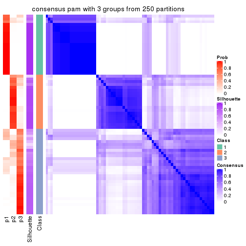
consensus_heatmap(res, k = 4)
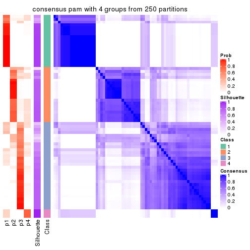
consensus_heatmap(res, k = 5)
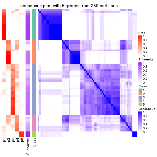
consensus_heatmap(res, k = 6)
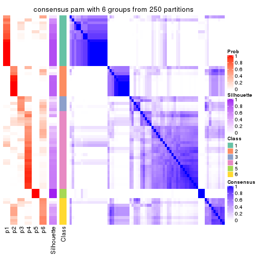
Heatmaps for the membership of samples in all partitions to see how consistent they are:
membership_heatmap(res, k = 2)
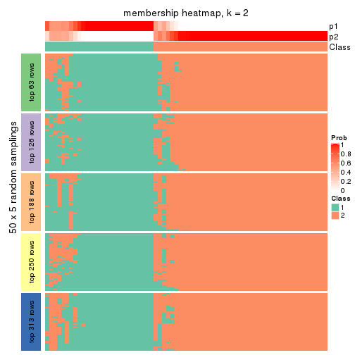
membership_heatmap(res, k = 3)
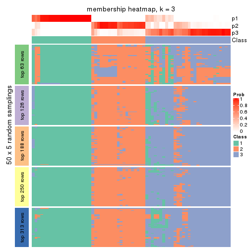
membership_heatmap(res, k = 4)
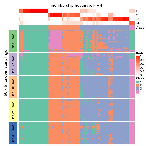
membership_heatmap(res, k = 5)
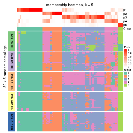
membership_heatmap(res, k = 6)
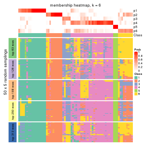
As soon as we have had the classes for columns, we can look for signatures which are significantly different between classes which can be candidate marks for certain classes. Following are the heatmaps for signatures.
Signature heatmaps where rows are scaled:
get_signatures(res, k = 2)
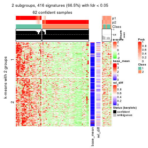
get_signatures(res, k = 3)
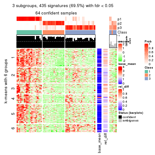
get_signatures(res, k = 4)
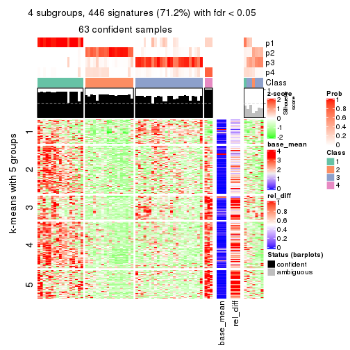
get_signatures(res, k = 5)
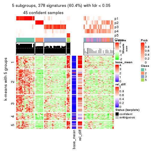
get_signatures(res, k = 6)
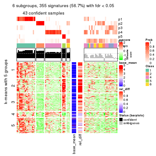
Signature heatmaps where rows are not scaled:
get_signatures(res, k = 2, scale_rows = FALSE)
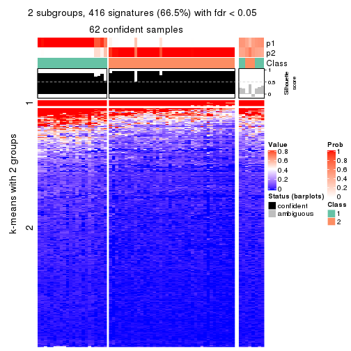
get_signatures(res, k = 3, scale_rows = FALSE)
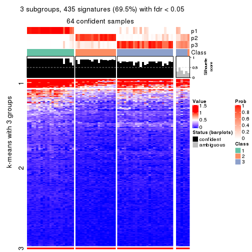
get_signatures(res, k = 4, scale_rows = FALSE)
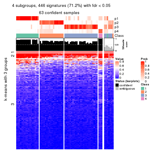
get_signatures(res, k = 5, scale_rows = FALSE)
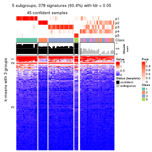
get_signatures(res, k = 6, scale_rows = FALSE)
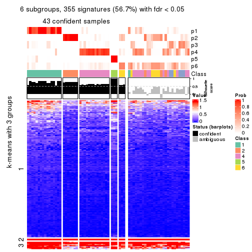
Compare the overlap of signatures from different k:
compare_signatures(res)
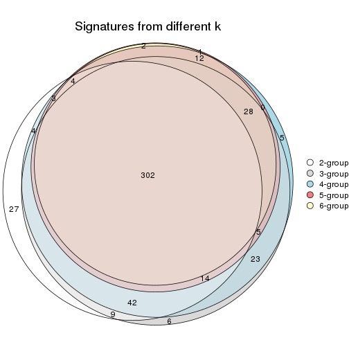
get_signature() returns a data frame invisibly. TO get the list of signatures, the function
call should be assigned to a variable explicitly. In following code, if plot argument is set
to FALSE, no heatmap is plotted while only the differential analysis is performed.
# code only for demonstration
tb = get_signature(res, k = ..., plot = FALSE)
An example of the output of tb is:
#>   which_row         fdr    mean_1    mean_2 scaled_mean_1 scaled_mean_2 km
#> 1        38 0.042760348  8.373488  9.131774    -0.5533452     0.5164555  1
#> 2        40 0.018707592  7.106213  8.469186    -0.6173731     0.5762149  1
#> 3        55 0.019134737 10.221463 11.207825    -0.6159697     0.5749050  1
#> 4        59 0.006059896  5.921854  7.869574    -0.6899429     0.6439467  1
#> 5        60 0.018055526  8.928898 10.211722    -0.6204761     0.5791110  1
#> 6        98 0.009384629 15.714769 14.887706     0.6635654    -0.6193277  2
...
The columns in tb are:
which_row: row indices corresponding to the input matrix.fdr: FDR for the differential test. mean_x: The mean value in group x.scaled_mean_x: The mean value in group x after rows are scaled.km: Row groups if k-means clustering is applied to rows.UMAP plot which shows how samples are separated.
dimension_reduction(res, k = 2, method = "UMAP")
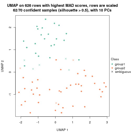
dimension_reduction(res, k = 3, method = "UMAP")
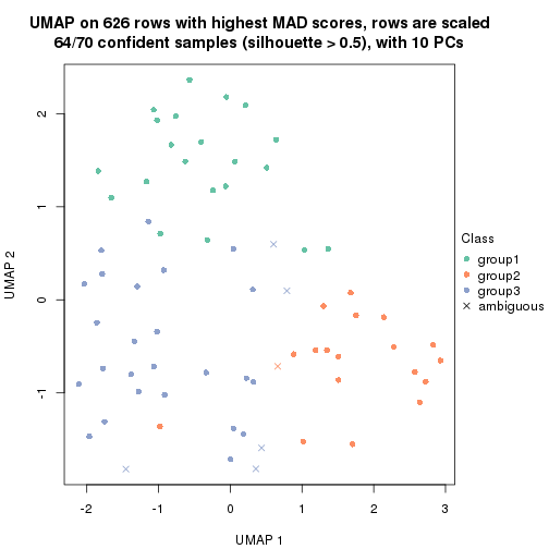
dimension_reduction(res, k = 4, method = "UMAP")
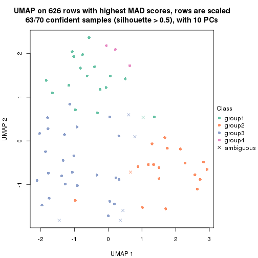
dimension_reduction(res, k = 5, method = "UMAP")
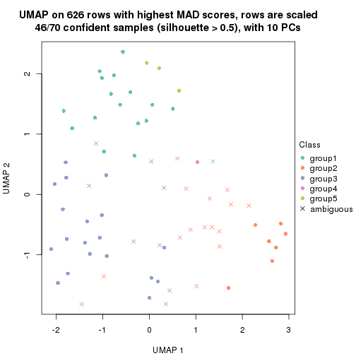
dimension_reduction(res, k = 6, method = "UMAP")
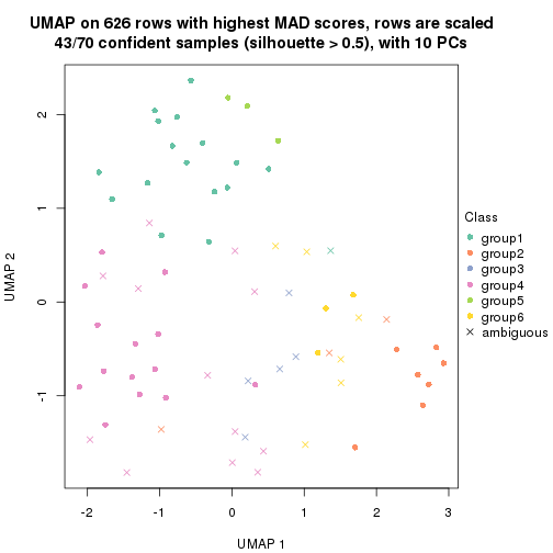
Following heatmap shows how subgroups are split when increasing k:
collect_classes(res)
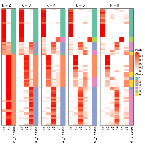
If matrix rows can be associated to genes, consider to use functional_enrichment(res,
...) to perform function enrichment for the signature genes. See this vignette for more detailed explanations.
The object with results only for a single top-value method and a single partition method can be extracted as:
res = res_list["MAD", "mclust"]
# you can also extract it by
# res = res_list["MAD:mclust"]
A summary of res and all the functions that can be applied to it:
res
#> A 'ConsensusPartition' object with k = 2, 3, 4, 5, 6.
#>   On a matrix with 626 rows and 70 columns.
#>   Top rows (63, 126, 188, 250, 313) are extracted by 'MAD' method.
#>   Subgroups are detected by 'mclust' method.
#>   Performed in total 1250 partitions by row resampling.
#>   Best k for subgroups seems to be 5.
#>
#> Following methods can be applied to this 'ConsensusPartition' object:
#>  [1] "cola_report"             "collect_classes"         "collect_plots"
#>  [4] "collect_stats"           "colnames"                "compare_signatures"
#>  [7] "consensus_heatmap"       "dimension_reduction"     "functional_enrichment"
#> [10] "get_anno_col"            "get_anno"                "get_classes"
#> [13] "get_consensus"           "get_matrix"              "get_membership"
#> [16] "get_param"               "get_signatures"          "get_stats"
#> [19] "is_best_k"               "is_stable_k"             "membership_heatmap"
#> [22] "ncol"                    "nrow"                    "plot_ecdf"
#> [25] "rownames"                "select_partition_number" "show"
#> [28] "suggest_best_k"          "test_to_known_factors"
collect_plots() function collects all the plots made from res for all k (number of partitions)
into one single page to provide an easy and fast comparison between different k.
collect_plots(res)
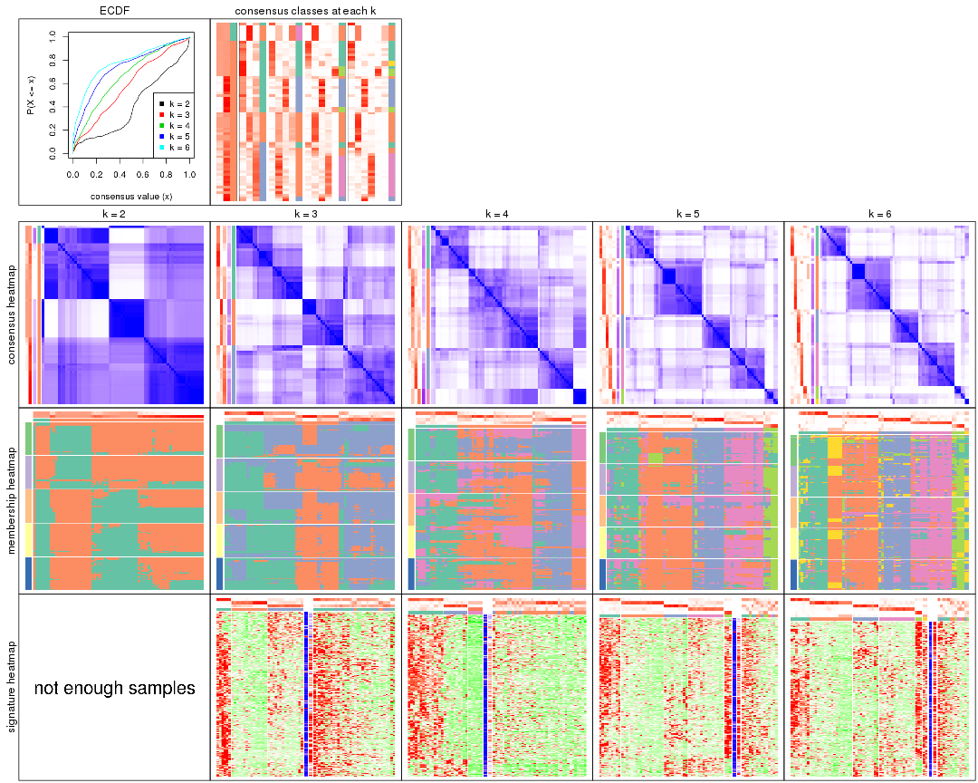
The plots are:
k and the heatmap of
predicted classes for each k.k.k.k.All the plots in panels can be made by individual functions and they are plotted later in this section.
select_partition_number() produces several plots showing different
statistics for choosing “optimized” k. There are following statistics:
k;k, the area increased is defined as \(A_k - A_{k-1}\).The detailed explanations of these statistics can be found in the cola vignette.
Generally speaking, lower PAC score, higher mean silhouette score or higher
concordance corresponds to better partition. Rand index and Jaccard index
measure how similar the current partition is compared to partition with k-1.
If they are too similar, we won't accept k is better than k-1.
select_partition_number(res)
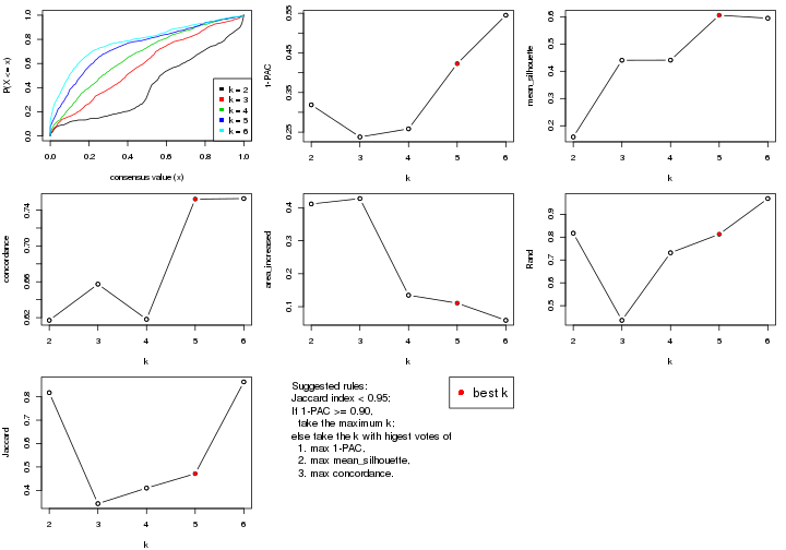
The numeric values for all these statistics can be obtained by get_stats().
get_stats(res)
#>   k 1-PAC mean_silhouette concordance area_increased  Rand Jaccard
#> 2 2 0.319           0.159       0.617         0.4115 0.817   0.817
#> 3 3 0.238           0.440       0.657         0.4278 0.436   0.343
#> 4 4 0.258           0.441       0.618         0.1348 0.732   0.410
#> 5 5 0.423           0.606       0.752         0.1107 0.813   0.471
#> 6 6 0.545           0.595       0.753         0.0587 0.969   0.863
suggest_best_k() suggests the best \(k\) based on these statistics. The rules are as follows:
suggest_best_k(res)
#> [1] 5
Following shows the table of the partitions (You need to click the show/hide
code output link to see it). The membership matrix (columns with name p*)
is inferred by
clue::cl_consensus()
function with the SE method. Basically the value in the membership matrix
represents the probability to belong to a certain group. The finall class
label for an item is determined with the group with highest probability it
belongs to.
In get_classes() function, the entropy is calculated from the membership
matrix and the silhouette score is calculated from the consensus matrix.
cbind(get_classes(res, k = 2), get_membership(res, k = 2))
#>           class entropy silhouette    p1    p2
#> SRR837437     2  0.9896   -0.57394 0.440 0.560
#> SRR837438     2  0.4431    0.44179 0.092 0.908
#> SRR837439     2  0.4562    0.35304 0.096 0.904
#> SRR837440     2  0.8016   -0.00527 0.244 0.756
#> SRR837441     2  0.7139    0.16041 0.196 0.804
#> SRR837442     2  0.9977   -0.65244 0.472 0.528
#> SRR837443     2  0.8327   -0.08123 0.264 0.736
#> SRR837444     2  0.4815    0.33032 0.104 0.896
#> SRR837445     2  0.9608   -0.43842 0.384 0.616
#> SRR837446     2  0.0672    0.43931 0.008 0.992
#> SRR837447     2  0.9993    0.32248 0.484 0.516
#> SRR837448     2  0.9993    0.32248 0.484 0.516
#> SRR837449     1  1.0000   -0.42367 0.500 0.500
#> SRR837450     2  0.9993    0.32248 0.484 0.516
#> SRR837451     1  0.9993    0.70467 0.516 0.484
#> SRR837452     2  0.9775   -0.51120 0.412 0.588
#> SRR837453     1  0.9993    0.70467 0.516 0.484
#> SRR837454     2  1.0000   -0.70454 0.496 0.504
#> SRR837455     2  0.9998    0.32116 0.492 0.508
#> SRR837456     2  0.9998    0.32116 0.492 0.508
#> SRR837457     1  0.9993    0.70467 0.516 0.484
#> SRR837458     2  0.9996    0.32181 0.488 0.512
#> SRR837459     1  0.9996    0.69657 0.512 0.488
#> SRR837460     1  0.9993    0.70467 0.516 0.484
#> SRR837461     2  0.7528    0.08539 0.216 0.784
#> SRR837462     2  0.2948    0.45077 0.052 0.948
#> SRR837463     2  0.4298    0.44606 0.088 0.912
#> SRR837464     2  0.1843    0.42644 0.028 0.972
#> SRR837465     2  0.4431    0.36605 0.092 0.908
#> SRR837466     2  0.9993    0.32248 0.484 0.516
#> SRR837467     2  0.9896   -0.57195 0.440 0.560
#> SRR837468     2  0.3431    0.44867 0.064 0.936
#> SRR837469     2  0.9993    0.32248 0.484 0.516
#> SRR837470     2  0.9993    0.32248 0.484 0.516
#> SRR837471     2  1.0000   -0.70454 0.496 0.504
#> SRR837472     2  1.0000   -0.70454 0.496 0.504
#> SRR837473     2  0.7299    0.20044 0.204 0.796
#> SRR837474     2  1.0000   -0.70454 0.496 0.504
#> SRR837475     2  0.9866   -0.55151 0.432 0.568
#> SRR837476     2  1.0000   -0.70454 0.496 0.504
#> SRR837477     2  0.2423    0.44945 0.040 0.960
#> SRR837478     2  0.0000    0.44399 0.000 1.000
#> SRR837479     2  0.0000    0.44399 0.000 1.000
#> SRR837480     2  0.0376    0.44177 0.004 0.996
#> SRR837481     2  0.0000    0.44399 0.000 1.000
#> SRR837482     2  0.4939    0.43750 0.108 0.892
#> SRR837483     2  0.9922    0.33134 0.448 0.552
#> SRR837484     2  0.0938    0.43660 0.012 0.988
#> SRR837485     2  0.0672    0.43931 0.008 0.992
#> SRR837486     2  0.0672    0.44613 0.008 0.992
#> SRR837487     2  0.9000   -0.23566 0.316 0.684
#> SRR837488     1  0.9993    0.70467 0.516 0.484
#> SRR837489     2  0.9998   -0.69785 0.492 0.508
#> SRR837490     2  1.0000   -0.70454 0.496 0.504
#> SRR837491     2  0.6048    0.26964 0.148 0.852
#> SRR837492     2  0.2603    0.45056 0.044 0.956
#> SRR837493     2  0.4298    0.44606 0.088 0.912
#> SRR837494     2  0.9833   -0.53395 0.424 0.576
#> SRR837495     2  0.9129   -0.28156 0.328 0.672
#> SRR837496     2  0.9993    0.32248 0.484 0.516
#> SRR837497     2  0.9996    0.32201 0.488 0.512
#> SRR837498     2  0.9993    0.32248 0.484 0.516
#> SRR837499     2  1.0000    0.31677 0.500 0.500
#> SRR837500     2  0.8327    0.39285 0.264 0.736
#> SRR837501     2  0.0000    0.44399 0.000 1.000
#> SRR837502     2  0.7745    0.40569 0.228 0.772
#> SRR837503     2  0.9998    0.32116 0.492 0.508
#> SRR837504     2  0.1633    0.42840 0.024 0.976
#> SRR837505     2  0.0000    0.44399 0.000 1.000
#> SRR837506     2  0.0000    0.44399 0.000 1.000
cbind(get_classes(res, k = 3), get_membership(res, k = 3))
#>           class entropy silhouette    p1    p2    p3
#> SRR837437     3  0.5859     0.3373 0.000 0.344 0.656
#> SRR837438     3  0.6848     0.6194 0.164 0.100 0.736
#> SRR837439     3  0.6354     0.6252 0.052 0.204 0.744
#> SRR837440     3  0.4784     0.5826 0.004 0.200 0.796
#> SRR837441     3  0.4931     0.5773 0.004 0.212 0.784
#> SRR837442     2  0.7067     0.5094 0.028 0.596 0.376
#> SRR837443     3  0.5842     0.6139 0.036 0.196 0.768
#> SRR837444     3  0.6918     0.6474 0.136 0.128 0.736
#> SRR837445     3  0.8659     0.2481 0.104 0.408 0.488
#> SRR837446     1  0.7748     0.2313 0.500 0.048 0.452
#> SRR837447     1  0.4353     0.4430 0.836 0.008 0.156
#> SRR837448     1  0.0892     0.5019 0.980 0.020 0.000
#> SRR837449     1  0.6704     0.2118 0.608 0.016 0.376
#> SRR837450     1  0.0892     0.5019 0.980 0.020 0.000
#> SRR837451     2  0.0892     0.6749 0.000 0.980 0.020
#> SRR837452     2  0.7580     0.4895 0.056 0.604 0.340
#> SRR837453     2  0.0892     0.6749 0.000 0.980 0.020
#> SRR837454     2  0.5874     0.7318 0.032 0.760 0.208
#> SRR837455     1  0.6584     0.2167 0.608 0.012 0.380
#> SRR837456     1  0.6814     0.2261 0.608 0.020 0.372
#> SRR837457     2  0.0892     0.6749 0.000 0.980 0.020
#> SRR837458     1  0.4409     0.4312 0.824 0.004 0.172
#> SRR837459     2  0.1267     0.6774 0.004 0.972 0.024
#> SRR837460     2  0.0892     0.6749 0.000 0.980 0.020
#> SRR837461     3  0.4784     0.5849 0.004 0.200 0.796
#> SRR837462     3  0.4749     0.5070 0.172 0.012 0.816
#> SRR837463     3  0.5581     0.5405 0.176 0.036 0.788
#> SRR837464     3  0.6004     0.6034 0.156 0.064 0.780
#> SRR837465     3  0.7828     0.6425 0.168 0.160 0.672
#> SRR837466     1  0.0892     0.5019 0.980 0.020 0.000
#> SRR837467     3  0.5678     0.4009 0.000 0.316 0.684
#> SRR837468     1  0.6252     0.3218 0.556 0.000 0.444
#> SRR837469     1  0.1267     0.5004 0.972 0.004 0.024
#> SRR837470     1  0.0829     0.5022 0.984 0.004 0.012
#> SRR837471     2  0.6183     0.7135 0.032 0.732 0.236
#> SRR837472     2  0.5921     0.7315 0.032 0.756 0.212
#> SRR837473     3  0.8593     0.6178 0.156 0.248 0.596
#> SRR837474     2  0.6099     0.7237 0.032 0.740 0.228
#> SRR837475     2  0.6977     0.6806 0.076 0.712 0.212
#> SRR837476     2  0.5860     0.7288 0.024 0.748 0.228
#> SRR837477     1  0.8464     0.2130 0.592 0.128 0.280
#> SRR837478     1  0.8914     0.1261 0.556 0.164 0.280
#> SRR837479     1  0.6505     0.3013 0.528 0.004 0.468
#> SRR837480     1  0.8962     0.1191 0.548 0.164 0.288
#> SRR837481     1  0.6495     0.3071 0.536 0.004 0.460
#> SRR837482     1  0.6252     0.3233 0.556 0.000 0.444
#> SRR837483     1  0.3551     0.4804 0.868 0.000 0.132
#> SRR837484     3  0.9108     0.0472 0.416 0.140 0.444
#> SRR837485     1  0.8521     0.1088 0.468 0.092 0.440
#> SRR837486     1  0.6267     0.3139 0.548 0.000 0.452
#> SRR837487     2  0.7597     0.3815 0.048 0.568 0.384
#> SRR837488     2  0.1289     0.6808 0.000 0.968 0.032
#> SRR837489     2  0.6793     0.6291 0.036 0.672 0.292
#> SRR837490     2  0.5921     0.7315 0.032 0.756 0.212
#> SRR837491     3  0.7756     0.6479 0.128 0.200 0.672
#> SRR837492     1  0.9211     0.0336 0.512 0.176 0.312
#> SRR837493     3  0.6174     0.5858 0.168 0.064 0.768
#> SRR837494     3  0.6189     0.2988 0.004 0.364 0.632
#> SRR837495     2  0.8875     0.1112 0.128 0.508 0.364
#> SRR837496     1  0.1315     0.5016 0.972 0.020 0.008
#> SRR837497     1  0.5953     0.3295 0.708 0.012 0.280
#> SRR837498     1  0.6448     0.2469 0.636 0.012 0.352
#> SRR837499     1  0.6704     0.2013 0.608 0.016 0.376
#> SRR837500     3  0.8391     0.1690 0.432 0.084 0.484
#> SRR837501     1  0.6291     0.3040 0.532 0.000 0.468
#> SRR837502     3  0.7150     0.3770 0.348 0.036 0.616
#> SRR837503     1  0.6859     0.2346 0.620 0.024 0.356
#> SRR837504     3  0.6726     0.6302 0.132 0.120 0.748
#> SRR837505     3  0.6521    -0.3219 0.496 0.004 0.500
#> SRR837506     1  0.6305     0.2911 0.516 0.000 0.484
cbind(get_classes(res, k = 4), get_membership(res, k = 4))
#>           class entropy silhouette    p1    p2    p3    p4
#> SRR837437     2   0.164     0.3614 0.000 0.940 0.000 0.060
#> SRR837438     2   0.819     0.3301 0.176 0.548 0.216 0.060
#> SRR837439     2   0.505     0.4700 0.080 0.800 0.092 0.028
#> SRR837440     2   0.337     0.4269 0.008 0.872 0.100 0.020
#> SRR837441     2   0.219     0.4053 0.048 0.932 0.012 0.008
#> SRR837442     2   0.617     0.1203 0.008 0.636 0.060 0.296
#> SRR837443     2   0.403     0.4690 0.008 0.796 0.192 0.004
#> SRR837444     2   0.698     0.3901 0.076 0.616 0.272 0.036
#> SRR837445     2   0.824     0.1843 0.048 0.480 0.144 0.328
#> SRR837446     3   0.446     0.6654 0.008 0.196 0.780 0.016
#> SRR837447     1   0.418     0.7121 0.848 0.028 0.080 0.044
#> SRR837448     1   0.641     0.5618 0.636 0.000 0.124 0.240
#> SRR837449     1   0.456     0.6984 0.816 0.088 0.008 0.088
#> SRR837450     1   0.639     0.5619 0.640 0.000 0.124 0.236
#> SRR837451     4   0.452     0.9917 0.000 0.320 0.000 0.680
#> SRR837452     2   0.802     0.0644 0.032 0.468 0.144 0.356
#> SRR837453     4   0.452     0.9917 0.000 0.320 0.000 0.680
#> SRR837454     2   0.738    -0.1521 0.016 0.452 0.104 0.428
#> SRR837455     1   0.411     0.7177 0.844 0.052 0.012 0.092
#> SRR837456     1   0.417     0.7179 0.840 0.052 0.012 0.096
#> SRR837457     4   0.452     0.9917 0.000 0.320 0.000 0.680
#> SRR837458     1   0.483     0.7070 0.816 0.056 0.088 0.040
#> SRR837459     4   0.470     0.9839 0.000 0.320 0.004 0.676
#> SRR837460     4   0.452     0.9917 0.000 0.320 0.000 0.680
#> SRR837461     2   0.344     0.4205 0.016 0.872 0.096 0.016
#> SRR837462     2   0.783     0.2410 0.116 0.532 0.308 0.044
#> SRR837463     2   0.858     0.2662 0.220 0.496 0.220 0.064
#> SRR837464     2   0.651     0.3650 0.052 0.652 0.260 0.036
#> SRR837465     2   0.849     0.4349 0.128 0.552 0.172 0.148
#> SRR837466     1   0.641     0.5618 0.636 0.000 0.124 0.240
#> SRR837467     2   0.187     0.3564 0.000 0.928 0.000 0.072
#> SRR837468     3   0.384     0.6936 0.092 0.052 0.852 0.004
#> SRR837469     1   0.579     0.5311 0.648 0.004 0.304 0.044
#> SRR837470     1   0.577     0.5365 0.652 0.004 0.300 0.044
#> SRR837471     2   0.725    -0.1867 0.008 0.460 0.112 0.420
#> SRR837472     2   0.721    -0.1933 0.008 0.464 0.108 0.420
#> SRR837473     2   0.938     0.3207 0.232 0.432 0.160 0.176
#> SRR837474     2   0.717    -0.2011 0.008 0.468 0.104 0.420
#> SRR837475     2   0.852     0.0651 0.072 0.444 0.128 0.356
#> SRR837476     2   0.639    -0.2927 0.000 0.528 0.068 0.404
#> SRR837477     3   0.930     0.4214 0.288 0.172 0.412 0.128
#> SRR837478     3   0.921     0.4301 0.224 0.224 0.440 0.112
#> SRR837479     3   0.238     0.7319 0.004 0.080 0.912 0.004
#> SRR837480     3   0.865     0.4816 0.192 0.224 0.504 0.080
#> SRR837481     3   0.246     0.7326 0.008 0.076 0.912 0.004
#> SRR837482     3   0.350     0.7111 0.060 0.056 0.876 0.008
#> SRR837483     3   0.670    -0.1510 0.460 0.024 0.476 0.040
#> SRR837484     3   0.602     0.4129 0.016 0.344 0.612 0.028
#> SRR837485     3   0.477     0.6446 0.012 0.216 0.756 0.016
#> SRR837486     3   0.264     0.7258 0.012 0.064 0.912 0.012
#> SRR837487     2   0.724     0.0430 0.016 0.520 0.100 0.364
#> SRR837488     4   0.460     0.9701 0.000 0.336 0.000 0.664
#> SRR837489     2   0.712    -0.1614 0.008 0.476 0.100 0.416
#> SRR837490     2   0.713    -0.2181 0.008 0.468 0.100 0.424
#> SRR837491     2   0.793     0.4239 0.116 0.608 0.136 0.140
#> SRR837492     3   0.972     0.2201 0.236 0.268 0.344 0.152
#> SRR837493     2   0.837     0.3119 0.200 0.524 0.216 0.060
#> SRR837494     2   0.314     0.3990 0.000 0.884 0.044 0.072
#> SRR837495     2   0.917     0.2572 0.124 0.444 0.168 0.264
#> SRR837496     1   0.601     0.6036 0.716 0.012 0.152 0.120
#> SRR837497     1   0.433     0.7225 0.844 0.044 0.068 0.044
#> SRR837498     1   0.545     0.6706 0.764 0.140 0.076 0.020
#> SRR837499     1   0.475     0.6917 0.804 0.096 0.008 0.092
#> SRR837500     1   0.821     0.3795 0.576 0.180 0.108 0.136
#> SRR837501     3   0.353     0.7195 0.024 0.104 0.864 0.008
#> SRR837502     1   0.888     0.0626 0.476 0.264 0.152 0.108
#> SRR837503     1   0.447     0.7176 0.820 0.068 0.008 0.104
#> SRR837504     2   0.605     0.1635 0.028 0.576 0.384 0.012
#> SRR837505     3   0.294     0.7295 0.012 0.088 0.892 0.008
#> SRR837506     3   0.273     0.7299 0.004 0.084 0.900 0.012
cbind(get_classes(res, k = 5), get_membership(res, k = 5))
#>           class entropy silhouette    p1    p2    p3    p4    p5
#> SRR837437     4  0.4240     0.6713 0.004 0.240 0.024 0.732 0.000
#> SRR837438     4  0.5514     0.6865 0.104 0.068 0.104 0.724 0.000
#> SRR837439     4  0.5416     0.7485 0.068 0.144 0.064 0.724 0.000
#> SRR837440     4  0.4252     0.7368 0.008 0.144 0.064 0.784 0.000
#> SRR837441     4  0.4623     0.7203 0.040 0.184 0.024 0.752 0.000
#> SRR837442     2  0.4941     0.4215 0.000 0.628 0.044 0.328 0.000
#> SRR837443     4  0.5258     0.7305 0.012 0.156 0.124 0.708 0.000
#> SRR837444     4  0.6811     0.6563 0.080 0.088 0.224 0.600 0.008
#> SRR837445     2  0.5057     0.7351 0.072 0.760 0.088 0.080 0.000
#> SRR837446     3  0.3963     0.6866 0.020 0.104 0.820 0.056 0.000
#> SRR837447     1  0.3802     0.5493 0.840 0.004 0.048 0.024 0.084
#> SRR837448     5  0.1952     0.6284 0.084 0.000 0.004 0.000 0.912
#> SRR837449     1  0.3648     0.6360 0.824 0.092 0.000 0.084 0.000
#> SRR837450     5  0.1952     0.6284 0.084 0.000 0.004 0.000 0.912
#> SRR837451     2  0.1671     0.7262 0.000 0.924 0.000 0.000 0.076
#> SRR837452     2  0.5112     0.7352 0.092 0.756 0.076 0.076 0.000
#> SRR837453     2  0.1671     0.7262 0.000 0.924 0.000 0.000 0.076
#> SRR837454     2  0.4010     0.7644 0.044 0.828 0.060 0.068 0.000
#> SRR837455     1  0.1831     0.6354 0.920 0.076 0.000 0.000 0.004
#> SRR837456     1  0.1831     0.6354 0.920 0.076 0.000 0.000 0.004
#> SRR837457     2  0.1671     0.7262 0.000 0.924 0.000 0.000 0.076
#> SRR837458     1  0.3363     0.6009 0.860 0.008 0.056 0.072 0.004
#> SRR837459     2  0.1671     0.7262 0.000 0.924 0.000 0.000 0.076
#> SRR837460     2  0.1671     0.7262 0.000 0.924 0.000 0.000 0.076
#> SRR837461     4  0.4480     0.7420 0.016 0.152 0.060 0.772 0.000
#> SRR837462     4  0.6529     0.5785 0.136 0.036 0.220 0.604 0.004
#> SRR837463     4  0.5105     0.6749 0.108 0.040 0.104 0.748 0.000
#> SRR837464     4  0.5491     0.7165 0.068 0.052 0.172 0.708 0.000
#> SRR837465     4  0.7273     0.5164 0.132 0.240 0.096 0.532 0.000
#> SRR837466     5  0.2929     0.5959 0.152 0.000 0.008 0.000 0.840
#> SRR837467     4  0.4252     0.6162 0.000 0.280 0.020 0.700 0.000
#> SRR837468     3  0.1503     0.7848 0.020 0.000 0.952 0.020 0.008
#> SRR837469     1  0.5727     0.2490 0.540 0.000 0.384 0.068 0.008
#> SRR837470     1  0.5560     0.1915 0.528 0.000 0.412 0.052 0.008
#> SRR837471     2  0.3477     0.7723 0.012 0.840 0.032 0.116 0.000
#> SRR837472     2  0.3160     0.7709 0.004 0.852 0.028 0.116 0.000
#> SRR837473     2  0.7660     0.4689 0.196 0.544 0.096 0.144 0.020
#> SRR837474     2  0.3160     0.7709 0.004 0.852 0.028 0.116 0.000
#> SRR837475     2  0.4827     0.7388 0.080 0.776 0.080 0.064 0.000
#> SRR837476     2  0.3659     0.7158 0.000 0.768 0.012 0.220 0.000
#> SRR837477     5  0.8028     0.4587 0.084 0.120 0.196 0.064 0.536
#> SRR837478     5  0.8127     0.3540 0.044 0.180 0.236 0.060 0.480
#> SRR837479     3  0.0162     0.7893 0.000 0.000 0.996 0.004 0.000
#> SRR837480     3  0.8304    -0.0379 0.040 0.232 0.428 0.056 0.244
#> SRR837481     3  0.0324     0.7906 0.000 0.004 0.992 0.004 0.000
#> SRR837482     3  0.1549     0.7707 0.040 0.000 0.944 0.016 0.000
#> SRR837483     3  0.6306     0.2683 0.288 0.000 0.564 0.132 0.016
#> SRR837484     3  0.5989     0.4907 0.024 0.140 0.660 0.172 0.004
#> SRR837485     3  0.4447     0.6814 0.020 0.092 0.788 0.100 0.000
#> SRR837486     3  0.0579     0.7869 0.008 0.000 0.984 0.008 0.000
#> SRR837487     2  0.4815     0.7440 0.044 0.768 0.064 0.124 0.000
#> SRR837488     2  0.2069     0.7244 0.000 0.912 0.000 0.012 0.076
#> SRR837489     2  0.2932     0.7724 0.000 0.864 0.032 0.104 0.000
#> SRR837490     2  0.2848     0.7722 0.000 0.868 0.028 0.104 0.000
#> SRR837491     2  0.7416    -0.1035 0.112 0.440 0.092 0.356 0.000
#> SRR837492     2  0.9094    -0.0365 0.108 0.356 0.152 0.084 0.300
#> SRR837493     4  0.5560     0.6708 0.124 0.056 0.104 0.716 0.000
#> SRR837494     4  0.4430     0.6602 0.000 0.256 0.036 0.708 0.000
#> SRR837495     2  0.6049     0.7004 0.100 0.716 0.088 0.056 0.040
#> SRR837496     5  0.6962     0.2044 0.384 0.036 0.044 0.048 0.488
#> SRR837497     1  0.4498     0.6218 0.808 0.036 0.040 0.096 0.020
#> SRR837498     1  0.6197     0.3727 0.552 0.012 0.076 0.348 0.012
#> SRR837499     1  0.3754     0.6365 0.816 0.100 0.000 0.084 0.000
#> SRR837500     1  0.6445     0.5199 0.660 0.124 0.064 0.140 0.012
#> SRR837501     3  0.1883     0.7867 0.012 0.000 0.932 0.048 0.008
#> SRR837502     1  0.7372     0.3608 0.524 0.224 0.092 0.160 0.000
#> SRR837503     1  0.6052     0.5473 0.700 0.132 0.016 0.068 0.084
#> SRR837504     4  0.6914     0.3654 0.024 0.140 0.376 0.456 0.004
#> SRR837505     3  0.1644     0.7862 0.008 0.000 0.940 0.048 0.004
#> SRR837506     3  0.0963     0.7885 0.000 0.000 0.964 0.036 0.000
cbind(get_classes(res, k = 6), get_membership(res, k = 6))
#>           class entropy silhouette    p1    p2    p3    p4    p5    p6
#> SRR837437     4  0.3113    0.73308 0.000 0.144 0.004 0.828 0.020 0.004
#> SRR837438     4  0.4425    0.74489 0.068 0.040 0.108 0.776 0.004 0.004
#> SRR837439     4  0.3520    0.77396 0.016 0.084 0.052 0.836 0.000 0.012
#> SRR837440     4  0.2376    0.74697 0.004 0.044 0.020 0.908 0.020 0.004
#> SRR837441     4  0.3063    0.75391 0.012 0.088 0.008 0.864 0.020 0.008
#> SRR837442     2  0.4214    0.05152 0.000 0.528 0.004 0.460 0.000 0.008
#> SRR837443     4  0.3300    0.75767 0.000 0.060 0.080 0.844 0.008 0.008
#> SRR837444     4  0.5808    0.62606 0.028 0.056 0.240 0.636 0.008 0.032
#> SRR837445     2  0.4460    0.69372 0.048 0.796 0.080 0.044 0.016 0.016
#> SRR837446     3  0.3666    0.70378 0.004 0.052 0.832 0.076 0.004 0.032
#> SRR837447     1  0.3591    0.52384 0.812 0.000 0.016 0.000 0.052 0.120
#> SRR837448     5  0.1387    0.57968 0.068 0.000 0.000 0.000 0.932 0.000
#> SRR837449     1  0.1059    0.65630 0.964 0.016 0.000 0.016 0.004 0.000
#> SRR837450     5  0.1387    0.57968 0.068 0.000 0.000 0.000 0.932 0.000
#> SRR837451     2  0.3819    0.65699 0.000 0.652 0.000 0.008 0.000 0.340
#> SRR837452     2  0.3102    0.72693 0.036 0.876 0.028 0.036 0.004 0.020
#> SRR837453     2  0.3819    0.65699 0.000 0.652 0.000 0.008 0.000 0.340
#> SRR837454     2  0.2521    0.73931 0.024 0.904 0.028 0.032 0.004 0.008
#> SRR837455     1  0.1003    0.64750 0.964 0.004 0.000 0.000 0.004 0.028
#> SRR837456     1  0.1003    0.64750 0.964 0.004 0.000 0.000 0.004 0.028
#> SRR837457     2  0.3819    0.65699 0.000 0.652 0.000 0.008 0.000 0.340
#> SRR837458     1  0.4032    0.26925 0.704 0.000 0.020 0.004 0.004 0.268
#> SRR837459     2  0.3819    0.65699 0.000 0.652 0.000 0.008 0.000 0.340
#> SRR837460     2  0.3819    0.65699 0.000 0.652 0.000 0.008 0.000 0.340
#> SRR837461     4  0.1854    0.74543 0.004 0.028 0.016 0.932 0.020 0.000
#> SRR837462     4  0.5985    0.55877 0.088 0.012 0.224 0.624 0.008 0.044
#> SRR837463     4  0.4215    0.73891 0.068 0.028 0.108 0.788 0.004 0.004
#> SRR837464     4  0.3118    0.74699 0.020 0.012 0.124 0.840 0.004 0.000
#> SRR837465     4  0.6354    0.62632 0.100 0.200 0.104 0.588 0.008 0.000
#> SRR837466     5  0.2668    0.50012 0.168 0.000 0.004 0.000 0.828 0.000
#> SRR837467     4  0.3519    0.71824 0.000 0.164 0.008 0.800 0.020 0.008
#> SRR837468     3  0.3209    0.71925 0.008 0.004 0.852 0.036 0.008 0.092
#> SRR837469     6  0.6083    0.98549 0.324 0.000 0.204 0.004 0.004 0.464
#> SRR837470     6  0.6091    0.98539 0.328 0.000 0.204 0.004 0.004 0.460
#> SRR837471     2  0.1601    0.73305 0.004 0.944 0.004 0.028 0.004 0.016
#> SRR837472     2  0.1338    0.73491 0.000 0.952 0.004 0.032 0.004 0.008
#> SRR837473     2  0.6808    0.45897 0.256 0.556 0.084 0.060 0.024 0.020
#> SRR837474     2  0.1440    0.73466 0.000 0.948 0.004 0.032 0.004 0.012
#> SRR837475     2  0.3902    0.71243 0.056 0.832 0.048 0.036 0.016 0.012
#> SRR837476     2  0.2830    0.69519 0.000 0.836 0.000 0.144 0.020 0.000
#> SRR837477     5  0.8563    0.37966 0.104 0.088 0.196 0.036 0.428 0.148
#> SRR837478     5  0.8541    0.27118 0.036 0.156 0.268 0.040 0.364 0.136
#> SRR837479     3  0.1036    0.75198 0.000 0.000 0.964 0.008 0.004 0.024
#> SRR837480     3  0.8450   -0.08124 0.028 0.240 0.392 0.048 0.168 0.124
#> SRR837481     3  0.0951    0.75463 0.004 0.000 0.968 0.008 0.000 0.020
#> SRR837482     3  0.3099    0.72397 0.016 0.004 0.864 0.028 0.008 0.080
#> SRR837483     3  0.6684   -0.26316 0.204 0.004 0.488 0.040 0.004 0.260
#> SRR837484     3  0.5305    0.54620 0.004 0.100 0.672 0.196 0.004 0.024
#> SRR837485     3  0.3766    0.69633 0.004 0.044 0.820 0.100 0.004 0.028
#> SRR837486     3  0.2121    0.74723 0.000 0.004 0.916 0.032 0.008 0.040
#> SRR837487     2  0.4765    0.65315 0.012 0.732 0.108 0.136 0.004 0.008
#> SRR837488     2  0.3998    0.65546 0.000 0.644 0.000 0.016 0.000 0.340
#> SRR837489     2  0.1268    0.73918 0.000 0.952 0.008 0.036 0.004 0.000
#> SRR837490     2  0.0692    0.73789 0.000 0.976 0.004 0.020 0.000 0.000
#> SRR837491     4  0.6230    0.28356 0.060 0.392 0.080 0.464 0.004 0.000
#> SRR837492     2  0.9162   -0.16996 0.140 0.332 0.128 0.040 0.220 0.140
#> SRR837493     4  0.4726    0.74381 0.072 0.056 0.108 0.756 0.004 0.004
#> SRR837494     4  0.3393    0.74026 0.000 0.140 0.012 0.820 0.020 0.008
#> SRR837495     2  0.5826    0.63471 0.100 0.704 0.092 0.040 0.040 0.024
#> SRR837496     1  0.6326   -0.08668 0.432 0.008 0.028 0.004 0.416 0.112
#> SRR837497     1  0.3481    0.61859 0.852 0.024 0.016 0.032 0.008 0.068
#> SRR837498     1  0.6465   -0.00501 0.560 0.004 0.056 0.196 0.004 0.180
#> SRR837499     1  0.1232    0.65667 0.956 0.016 0.000 0.024 0.004 0.000
#> SRR837500     1  0.4760    0.51349 0.780 0.076 0.052 0.052 0.024 0.016
#> SRR837501     3  0.2848    0.73950 0.000 0.004 0.872 0.056 0.008 0.060
#> SRR837502     1  0.5753    0.39292 0.684 0.128 0.084 0.084 0.008 0.012
#> SRR837503     1  0.2969    0.63720 0.880 0.056 0.012 0.008 0.028 0.016
#> SRR837504     4  0.5628    0.46920 0.008 0.072 0.316 0.580 0.004 0.020
#> SRR837505     3  0.1296    0.75498 0.000 0.000 0.952 0.032 0.004 0.012
#> SRR837506     3  0.1485    0.75266 0.000 0.000 0.944 0.024 0.004 0.028
Heatmaps for the consensus matrix. It visualizes the probability of two samples to be in a same group.
consensus_heatmap(res, k = 2)
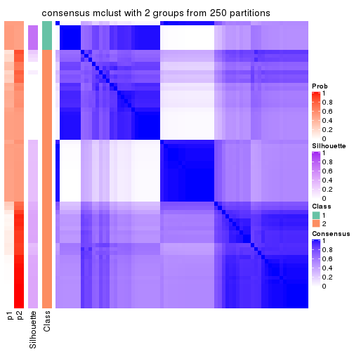
consensus_heatmap(res, k = 3)
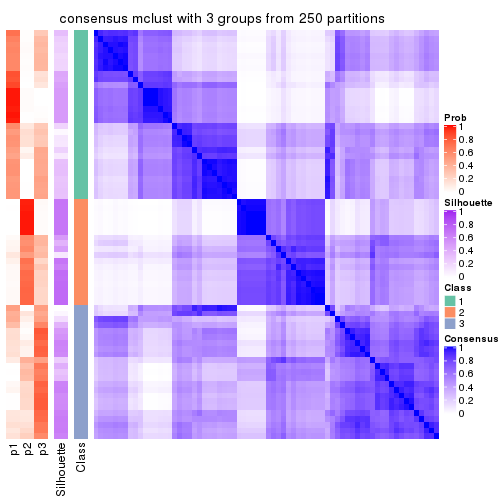
consensus_heatmap(res, k = 4)
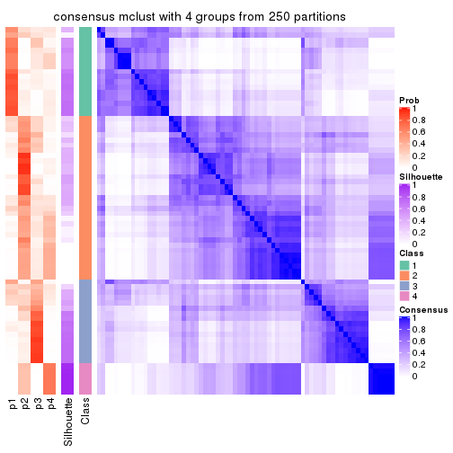
consensus_heatmap(res, k = 5)
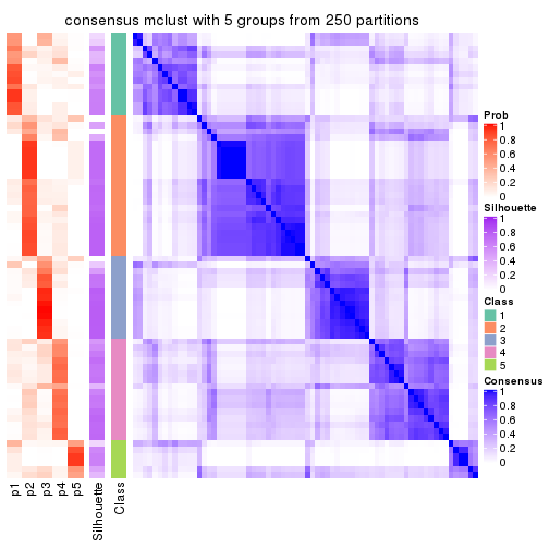
consensus_heatmap(res, k = 6)
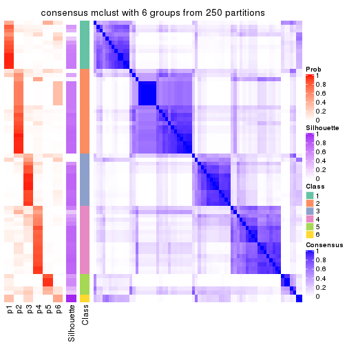
Heatmaps for the membership of samples in all partitions to see how consistent they are:
membership_heatmap(res, k = 2)
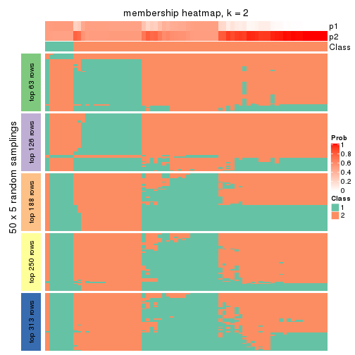
membership_heatmap(res, k = 3)
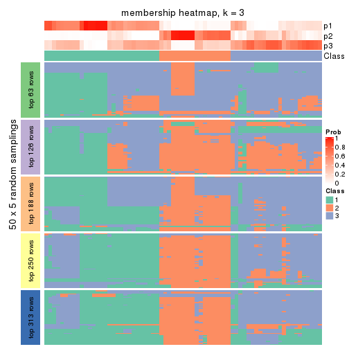
membership_heatmap(res, k = 4)
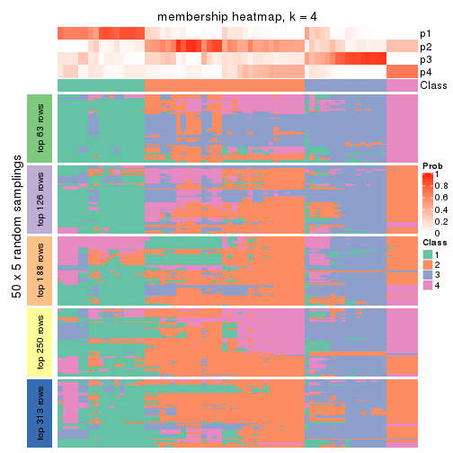
membership_heatmap(res, k = 5)
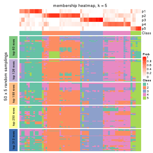
membership_heatmap(res, k = 6)
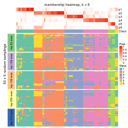
As soon as we have had the classes for columns, we can look for signatures which are significantly different between classes which can be candidate marks for certain classes. Following are the heatmaps for signatures.
Signature heatmaps where rows are scaled:
get_signatures(res, k = 2)

get_signatures(res, k = 3)
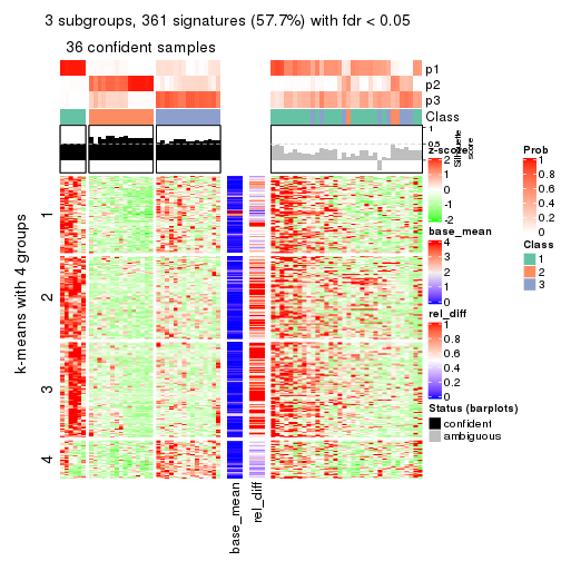
get_signatures(res, k = 4)
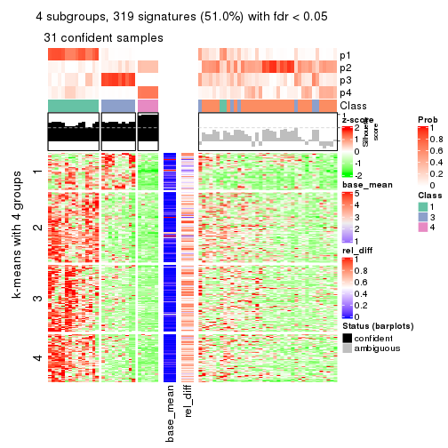
get_signatures(res, k = 5)
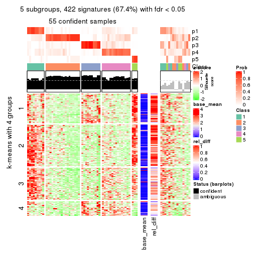
get_signatures(res, k = 6)
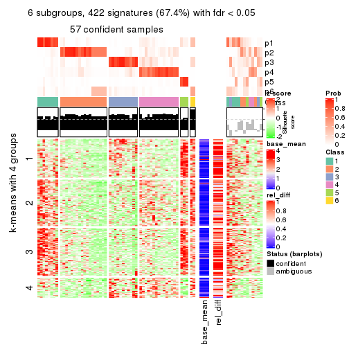
Signature heatmaps where rows are not scaled:
get_signatures(res, k = 2, scale_rows = FALSE)

get_signatures(res, k = 3, scale_rows = FALSE)
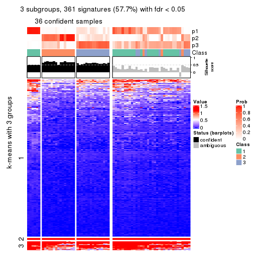
get_signatures(res, k = 4, scale_rows = FALSE)
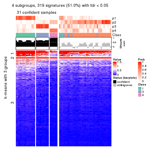
get_signatures(res, k = 5, scale_rows = FALSE)
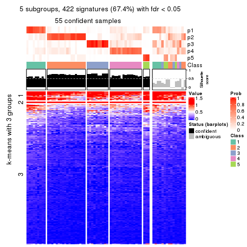
get_signatures(res, k = 6, scale_rows = FALSE)
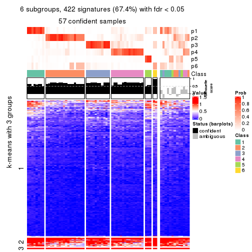
Compare the overlap of signatures from different k:
compare_signatures(res)
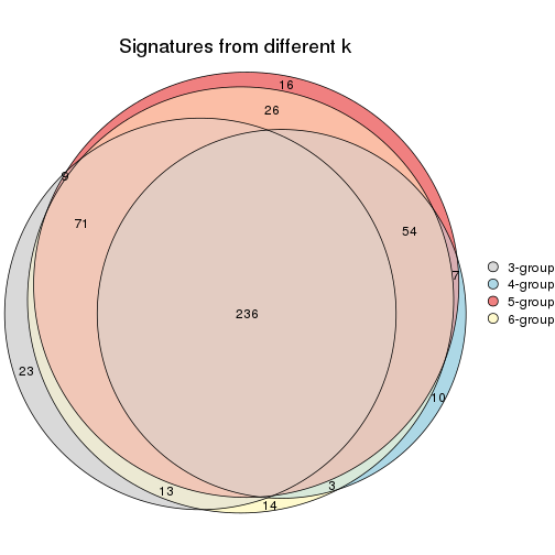
get_signature() returns a data frame invisibly. TO get the list of signatures, the function
call should be assigned to a variable explicitly. In following code, if plot argument is set
to FALSE, no heatmap is plotted while only the differential analysis is performed.
# code only for demonstration
tb = get_signature(res, k = ..., plot = FALSE)
An example of the output of tb is:
#>   which_row         fdr    mean_1    mean_2 scaled_mean_1 scaled_mean_2 km
#> 1        38 0.042760348  8.373488  9.131774    -0.5533452     0.5164555  1
#> 2        40 0.018707592  7.106213  8.469186    -0.6173731     0.5762149  1
#> 3        55 0.019134737 10.221463 11.207825    -0.6159697     0.5749050  1
#> 4        59 0.006059896  5.921854  7.869574    -0.6899429     0.6439467  1
#> 5        60 0.018055526  8.928898 10.211722    -0.6204761     0.5791110  1
#> 6        98 0.009384629 15.714769 14.887706     0.6635654    -0.6193277  2
...
The columns in tb are:
which_row: row indices corresponding to the input matrix.fdr: FDR for the differential test. mean_x: The mean value in group x.scaled_mean_x: The mean value in group x after rows are scaled.km: Row groups if k-means clustering is applied to rows.UMAP plot which shows how samples are separated.
dimension_reduction(res, k = 2, method = "UMAP")
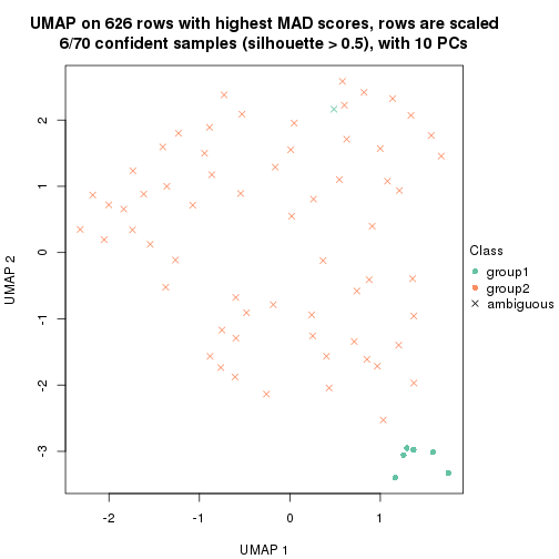
dimension_reduction(res, k = 3, method = "UMAP")
dimension_reduction(res, k = 4, method = "UMAP")
dimension_reduction(res, k = 5, method = "UMAP")
dimension_reduction(res, k = 6, method = "UMAP")
Following heatmap shows how subgroups are split when increasing k:
collect_classes(res)
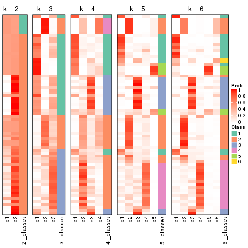
If matrix rows can be associated to genes, consider to use functional_enrichment(res,
...) to perform function enrichment for the signature genes. See this vignette for more detailed explanations.
The object with results only for a single top-value method and a single partition method can be extracted as:
res = res_list["MAD", "NMF"]
# you can also extract it by
# res = res_list["MAD:NMF"]
A summary of res and all the functions that can be applied to it:
res
#> A 'ConsensusPartition' object with k = 2, 3, 4, 5, 6.
#>   On a matrix with 626 rows and 70 columns.
#>   Top rows (63, 126, 188, 250, 313) are extracted by 'MAD' method.
#>   Subgroups are detected by 'NMF' method.
#>   Performed in total 1250 partitions by row resampling.
#>   Best k for subgroups seems to be 2.
#>
#> Following methods can be applied to this 'ConsensusPartition' object:
#>  [1] "cola_report"             "collect_classes"         "collect_plots"
#>  [4] "collect_stats"           "colnames"                "compare_signatures"
#>  [7] "consensus_heatmap"       "dimension_reduction"     "functional_enrichment"
#> [10] "get_anno_col"            "get_anno"                "get_classes"
#> [13] "get_consensus"           "get_matrix"              "get_membership"
#> [16] "get_param"               "get_signatures"          "get_stats"
#> [19] "is_best_k"               "is_stable_k"             "membership_heatmap"
#> [22] "ncol"                    "nrow"                    "plot_ecdf"
#> [25] "rownames"                "select_partition_number" "show"
#> [28] "suggest_best_k"          "test_to_known_factors"
collect_plots() function collects all the plots made from res for all k (number of partitions)
into one single page to provide an easy and fast comparison between different k.
collect_plots(res)
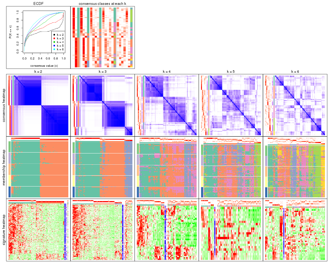
The plots are:
k and the heatmap of
predicted classes for each k.k.k.k.All the plots in panels can be made by individual functions and they are plotted later in this section.
select_partition_number() produces several plots showing different
statistics for choosing “optimized” k. There are following statistics:
k;k, the area increased is defined as \(A_k - A_{k-1}\).The detailed explanations of these statistics can be found in the cola vignette.
Generally speaking, lower PAC score, higher mean silhouette score or higher
concordance corresponds to better partition. Rand index and Jaccard index
measure how similar the current partition is compared to partition with k-1.
If they are too similar, we won't accept k is better than k-1.
select_partition_number(res)
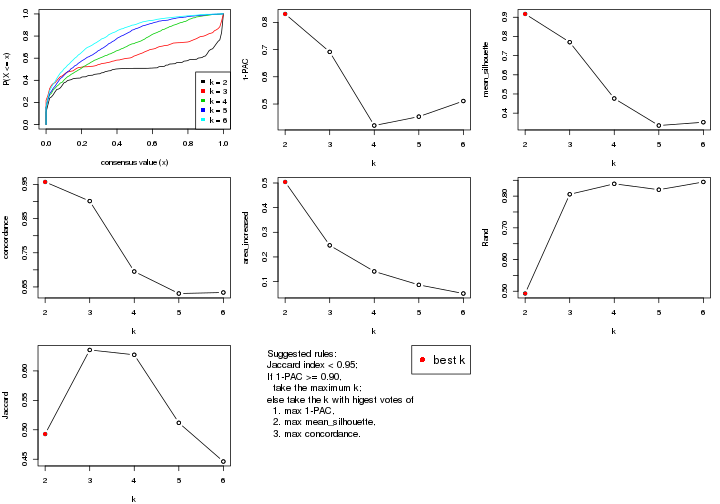
The numeric values for all these statistics can be obtained by get_stats().
get_stats(res)
#>   k 1-PAC mean_silhouette concordance area_increased  Rand Jaccard
#> 2 2 0.831           0.917       0.957         0.5042 0.493   0.493
#> 3 3 0.691           0.770       0.901         0.2470 0.806   0.636
#> 4 4 0.421           0.476       0.695         0.1412 0.839   0.627
#> 5 5 0.454           0.335       0.631         0.0867 0.820   0.512
#> 6 6 0.511           0.353       0.634         0.0516 0.845   0.446
suggest_best_k() suggests the best \(k\) based on these statistics. The rules are as follows:
suggest_best_k(res)
#> [1] 2
Following shows the table of the partitions (You need to click the show/hide
code output link to see it). The membership matrix (columns with name p*)
is inferred by
clue::cl_consensus()
function with the SE method. Basically the value in the membership matrix
represents the probability to belong to a certain group. The finall class
label for an item is determined with the group with highest probability it
belongs to.
In get_classes() function, the entropy is calculated from the membership
matrix and the silhouette score is calculated from the consensus matrix.
cbind(get_classes(res, k = 2), get_membership(res, k = 2))
#>           class entropy silhouette    p1    p2
#> SRR837437     2  0.1414      0.969 0.020 0.980
#> SRR837438     2  0.4022      0.925 0.080 0.920
#> SRR837439     2  0.2603      0.955 0.044 0.956
#> SRR837440     2  0.0672      0.972 0.008 0.992
#> SRR837441     2  0.2043      0.962 0.032 0.968
#> SRR837442     2  0.4161      0.921 0.084 0.916
#> SRR837443     2  0.0000      0.973 0.000 1.000
#> SRR837444     2  0.5059      0.879 0.112 0.888
#> SRR837445     1  0.2236      0.920 0.964 0.036
#> SRR837446     2  0.0000      0.973 0.000 1.000
#> SRR837447     1  0.0000      0.936 1.000 0.000
#> SRR837448     1  0.0000      0.936 1.000 0.000
#> SRR837449     1  0.0000      0.936 1.000 0.000
#> SRR837450     1  0.0938      0.931 0.988 0.012
#> SRR837451     2  0.0376      0.973 0.004 0.996
#> SRR837452     1  0.0000      0.936 1.000 0.000
#> SRR837453     2  0.3274      0.941 0.060 0.940
#> SRR837454     1  0.0000      0.936 1.000 0.000
#> SRR837455     1  0.0000      0.936 1.000 0.000
#> SRR837456     1  0.0000      0.936 1.000 0.000
#> SRR837457     2  0.0000      0.973 0.000 1.000
#> SRR837458     1  0.0000      0.936 1.000 0.000
#> SRR837459     2  0.0376      0.973 0.004 0.996
#> SRR837460     2  0.0000      0.973 0.000 1.000
#> SRR837461     2  0.0376      0.973 0.004 0.996
#> SRR837462     2  0.0672      0.972 0.008 0.992
#> SRR837463     2  0.1633      0.967 0.024 0.976
#> SRR837464     2  0.0938      0.971 0.012 0.988
#> SRR837465     1  0.4562      0.881 0.904 0.096
#> SRR837466     1  0.0000      0.936 1.000 0.000
#> SRR837467     2  0.1414      0.969 0.020 0.980
#> SRR837468     2  0.0000      0.973 0.000 1.000
#> SRR837469     2  0.7056      0.757 0.192 0.808
#> SRR837470     1  0.2778      0.915 0.952 0.048
#> SRR837471     1  0.0000      0.936 1.000 0.000
#> SRR837472     1  0.0000      0.936 1.000 0.000
#> SRR837473     1  0.0000      0.936 1.000 0.000
#> SRR837474     1  0.4298      0.885 0.912 0.088
#> SRR837475     1  0.0000      0.936 1.000 0.000
#> SRR837476     1  0.9491      0.463 0.632 0.368
#> SRR837477     1  0.1184      0.930 0.984 0.016
#> SRR837478     1  0.3114      0.910 0.944 0.056
#> SRR837479     2  0.0000      0.973 0.000 1.000
#> SRR837480     1  0.6048      0.840 0.852 0.148
#> SRR837481     2  0.0376      0.972 0.004 0.996
#> SRR837482     2  0.0376      0.972 0.004 0.996
#> SRR837483     1  0.7745      0.729 0.772 0.228
#> SRR837484     2  0.0000      0.973 0.000 1.000
#> SRR837485     2  0.0000      0.973 0.000 1.000
#> SRR837486     2  0.0000      0.973 0.000 1.000
#> SRR837487     2  0.4690      0.900 0.100 0.900
#> SRR837488     2  0.1414      0.969 0.020 0.980
#> SRR837489     1  0.9170      0.538 0.668 0.332
#> SRR837490     1  0.8909      0.588 0.692 0.308
#> SRR837491     1  0.8386      0.661 0.732 0.268
#> SRR837492     1  0.0000      0.936 1.000 0.000
#> SRR837493     2  0.2603      0.956 0.044 0.956
#> SRR837494     2  0.1184      0.970 0.016 0.984
#> SRR837495     1  0.0000      0.936 1.000 0.000
#> SRR837496     1  0.0000      0.936 1.000 0.000
#> SRR837497     1  0.0000      0.936 1.000 0.000
#> SRR837498     1  0.4161      0.888 0.916 0.084
#> SRR837499     1  0.0000      0.936 1.000 0.000
#> SRR837500     1  0.0000      0.936 1.000 0.000
#> SRR837501     2  0.0000      0.973 0.000 1.000
#> SRR837502     1  0.0000      0.936 1.000 0.000
#> SRR837503     1  0.0000      0.936 1.000 0.000
#> SRR837504     2  0.0000      0.973 0.000 1.000
#> SRR837505     2  0.0000      0.973 0.000 1.000
#> SRR837506     2  0.0000      0.973 0.000 1.000
cbind(get_classes(res, k = 3), get_membership(res, k = 3))
#>           class entropy silhouette    p1    p2    p3
#> SRR837437     2  0.0000    0.87781 0.000 1.000 0.000
#> SRR837438     2  0.0237    0.87680 0.004 0.996 0.000
#> SRR837439     2  0.0000    0.87781 0.000 1.000 0.000
#> SRR837440     2  0.0747    0.87345 0.000 0.984 0.016
#> SRR837441     2  0.0000    0.87781 0.000 1.000 0.000
#> SRR837442     2  0.0237    0.87679 0.004 0.996 0.000
#> SRR837443     2  0.0424    0.87685 0.000 0.992 0.008
#> SRR837444     2  0.2152    0.85008 0.036 0.948 0.016
#> SRR837445     1  0.3116    0.83334 0.892 0.108 0.000
#> SRR837446     3  0.4002    0.76967 0.000 0.160 0.840
#> SRR837447     1  0.0000    0.89071 1.000 0.000 0.000
#> SRR837448     1  0.3116    0.82079 0.892 0.000 0.108
#> SRR837449     1  0.0892    0.89283 0.980 0.020 0.000
#> SRR837450     1  0.4235    0.75450 0.824 0.000 0.176
#> SRR837451     2  0.0000    0.87781 0.000 1.000 0.000
#> SRR837452     1  0.0892    0.89283 0.980 0.020 0.000
#> SRR837453     2  0.2229    0.85090 0.012 0.944 0.044
#> SRR837454     1  0.0892    0.89297 0.980 0.020 0.000
#> SRR837455     1  0.1031    0.89200 0.976 0.024 0.000
#> SRR837456     1  0.0892    0.89283 0.980 0.020 0.000
#> SRR837457     2  0.0892    0.87449 0.000 0.980 0.020
#> SRR837458     1  0.0424    0.89214 0.992 0.008 0.000
#> SRR837459     2  0.0892    0.87418 0.000 0.980 0.020
#> SRR837460     2  0.0424    0.87756 0.000 0.992 0.008
#> SRR837461     2  0.0237    0.87752 0.000 0.996 0.004
#> SRR837462     2  0.0424    0.87779 0.000 0.992 0.008
#> SRR837463     2  0.0000    0.87781 0.000 1.000 0.000
#> SRR837464     2  0.0747    0.87407 0.000 0.984 0.016
#> SRR837465     1  0.5926    0.47356 0.644 0.356 0.000
#> SRR837466     1  0.0892    0.88339 0.980 0.000 0.020
#> SRR837467     2  0.0000    0.87781 0.000 1.000 0.000
#> SRR837468     2  0.5591    0.50999 0.000 0.696 0.304
#> SRR837469     2  0.8075    0.41829 0.104 0.620 0.276
#> SRR837470     1  0.4458    0.81942 0.864 0.056 0.080
#> SRR837471     1  0.1163    0.89075 0.972 0.028 0.000
#> SRR837472     1  0.1289    0.88898 0.968 0.032 0.000
#> SRR837473     1  0.0000    0.89071 1.000 0.000 0.000
#> SRR837474     1  0.4062    0.77614 0.836 0.164 0.000
#> SRR837475     1  0.0000    0.89071 1.000 0.000 0.000
#> SRR837476     1  0.6307    0.08582 0.512 0.488 0.000
#> SRR837477     1  0.6215    0.29528 0.572 0.000 0.428
#> SRR837478     3  0.2625    0.80039 0.084 0.000 0.916
#> SRR837479     3  0.0000    0.85019 0.000 0.000 1.000
#> SRR837480     3  0.1163    0.84222 0.028 0.000 0.972
#> SRR837481     3  0.0000    0.85019 0.000 0.000 1.000
#> SRR837482     2  0.6302   -0.00237 0.000 0.520 0.480
#> SRR837483     1  0.8013    0.33465 0.564 0.072 0.364
#> SRR837484     3  0.6307    0.03686 0.000 0.488 0.512
#> SRR837485     3  0.2165    0.84107 0.000 0.064 0.936
#> SRR837486     3  0.2796    0.82793 0.000 0.092 0.908
#> SRR837487     2  0.5428    0.73999 0.064 0.816 0.120
#> SRR837488     2  0.2066    0.84587 0.000 0.940 0.060
#> SRR837489     2  0.6204    0.24661 0.424 0.576 0.000
#> SRR837490     2  0.5497    0.54687 0.292 0.708 0.000
#> SRR837491     2  0.5988    0.39166 0.368 0.632 0.000
#> SRR837492     1  0.0747    0.88546 0.984 0.000 0.016
#> SRR837493     2  0.0000    0.87781 0.000 1.000 0.000
#> SRR837494     2  0.0237    0.87752 0.000 0.996 0.004
#> SRR837495     1  0.0000    0.89071 1.000 0.000 0.000
#> SRR837496     1  0.0000    0.89071 1.000 0.000 0.000
#> SRR837497     1  0.0000    0.89071 1.000 0.000 0.000
#> SRR837498     1  0.4293    0.77484 0.832 0.164 0.004
#> SRR837499     1  0.1031    0.89200 0.976 0.024 0.000
#> SRR837500     1  0.1031    0.89200 0.976 0.024 0.000
#> SRR837501     2  0.2796    0.82125 0.000 0.908 0.092
#> SRR837502     1  0.0892    0.89283 0.980 0.020 0.000
#> SRR837503     1  0.0000    0.89071 1.000 0.000 0.000
#> SRR837504     2  0.1753    0.85578 0.000 0.952 0.048
#> SRR837505     3  0.5497    0.59197 0.000 0.292 0.708
#> SRR837506     3  0.0000    0.85019 0.000 0.000 1.000
cbind(get_classes(res, k = 4), get_membership(res, k = 4))
#> class entropy silhouette p1 p2 p3 p4
#> SRR837437 2 0.336 0.5009 0.000 0.824 0.000 0.176
#> SRR837438 2 0.276 0.5440 0.044 0.904 0.000 0.052
#> SRR837439 2 0.152 0.5508 0.024 0.956 0.000 0.020
#> SRR837440 2 0.287 0.5410 0.000 0.864 0.000 0.136
#> SRR837441 2 0.108 0.5525 0.004 0.972 0.004 0.020
#> SRR837442 2 0.478 0.4160 0.016 0.712 0.000 0.272
#> SRR837443 2 0.213 0.5449 0.000 0.920 0.004 0.076
#> SRR837444 2 0.559 0.4651 0.104 0.772 0.044 0.080
#> SRR837445 2 0.734 0.3063 0.292 0.584 0.068 0.056
#> SRR837446 3 0.642 0.3798 0.000 0.228 0.640 0.132
#> SRR837447 1 0.543 0.7280 0.768 0.084 0.020 0.128
#> SRR837448 1 0.602 0.5583 0.632 0.000 0.300 0.068
#> SRR837449 1 0.371 0.7536 0.840 0.028 0.000 0.132
#> SRR837450 1 0.598 0.4393 0.580 0.000 0.372 0.048
#> SRR837451 2 0.503 0.4190 0.004 0.596 0.000 0.400
#> SRR837452 1 0.572 0.7163 0.736 0.080 0.016 0.168
#> SRR837453 2 0.643 0.4198 0.032 0.584 0.028 0.356
#> SRR837454 1 0.681 0.6279 0.644 0.208 0.016 0.132
#> SRR837455 1 0.292 0.7608 0.876 0.008 0.000 0.116
#> SRR837456 1 0.274 0.7636 0.888 0.008 0.000 0.104
#> SRR837457 2 0.523 0.4221 0.004 0.644 0.012 0.340
#> SRR837458 1 0.369 0.7559 0.856 0.000 0.064 0.080
#> SRR837459 2 0.472 0.4586 0.000 0.672 0.004 0.324
#> SRR837460 2 0.498 0.3857 0.000 0.612 0.004 0.384
#> SRR837461 2 0.480 0.3595 0.000 0.616 0.000 0.384
#> SRR837462 2 0.511 0.5024 0.052 0.736 0.000 0.212
#> SRR837463 2 0.462 0.4278 0.000 0.660 0.000 0.340
#> SRR837464 2 0.488 0.3268 0.000 0.592 0.000 0.408
#> SRR837465 2 0.706 0.0528 0.376 0.496 0.000 0.128
#> SRR837466 1 0.338 0.7405 0.860 0.000 0.116 0.024
#> SRR837467 2 0.438 0.4639 0.000 0.704 0.000 0.296
#> SRR837468 4 0.645 0.5225 0.000 0.204 0.152 0.644
#> SRR837469 2 0.914 0.1932 0.168 0.472 0.208 0.152
#> SRR837470 1 0.879 0.4325 0.492 0.184 0.232 0.092
#> SRR837471 1 0.221 0.7598 0.928 0.004 0.056 0.012
#> SRR837472 1 0.241 0.7565 0.916 0.000 0.064 0.020
#> SRR837473 1 0.256 0.7532 0.908 0.000 0.072 0.020
#> SRR837474 1 0.384 0.7367 0.848 0.116 0.012 0.024
#> SRR837475 1 0.218 0.7577 0.924 0.000 0.064 0.012
#> SRR837476 2 0.718 0.2826 0.336 0.512 0.000 0.152
#> SRR837477 3 0.515 0.2069 0.348 0.004 0.640 0.008
#> SRR837478 3 0.136 0.6028 0.032 0.000 0.960 0.008
#> SRR837479 3 0.265 0.5741 0.000 0.000 0.880 0.120
#> SRR837480 3 0.240 0.5998 0.048 0.000 0.920 0.032
#> SRR837481 3 0.271 0.5893 0.000 0.004 0.884 0.112
#> SRR837482 3 0.772 -0.3022 0.000 0.240 0.436 0.324
#> SRR837483 1 0.904 -0.0802 0.380 0.096 0.160 0.364
#> SRR837484 4 0.750 0.4595 0.000 0.300 0.212 0.488
#> SRR837485 3 0.602 0.2231 0.000 0.068 0.632 0.300
#> SRR837486 4 0.718 0.2183 0.000 0.140 0.380 0.480
#> SRR837487 4 0.773 0.1811 0.040 0.412 0.092 0.456
#> SRR837488 2 0.493 0.1102 0.000 0.568 0.000 0.432
#> SRR837489 2 0.622 0.4430 0.144 0.692 0.008 0.156
#> SRR837490 2 0.629 0.4380 0.184 0.688 0.012 0.116
#> SRR837491 2 0.705 0.3590 0.212 0.604 0.008 0.176
#> SRR837492 1 0.352 0.7202 0.852 0.004 0.128 0.016
#> SRR837493 2 0.380 0.5371 0.056 0.848 0.000 0.096
#> SRR837494 2 0.398 0.4893 0.000 0.760 0.000 0.240
#> SRR837495 1 0.695 0.6015 0.652 0.216 0.084 0.048
#> SRR837496 1 0.645 0.6592 0.700 0.072 0.180 0.048
#> SRR837497 1 0.595 0.6881 0.728 0.164 0.024 0.084
#> SRR837498 2 0.730 0.0529 0.372 0.504 0.012 0.112
#> SRR837499 1 0.438 0.7020 0.788 0.180 0.000 0.032
#> SRR837500 1 0.204 0.7746 0.940 0.036 0.008 0.016
#> SRR837501 4 0.515 0.3204 0.000 0.336 0.016 0.648
#> SRR837502 1 0.256 0.7661 0.912 0.068 0.004 0.016
#> SRR837503 1 0.229 0.7720 0.932 0.016 0.036 0.016
#> SRR837504 2 0.552 0.2826 0.000 0.596 0.024 0.380
#> SRR837505 4 0.622 0.4389 0.000 0.108 0.240 0.652
#> SRR837506 4 0.499 -0.1572 0.000 0.000 0.480 0.520
cbind(get_classes(res, k = 5), get_membership(res, k = 5))
#> class entropy silhouette p1 p2 p3 p4 p5
#> SRR837437 2 0.3854 0.46121 0.000 0.816 0.080 0.100 0.004
#> SRR837438 2 0.5166 0.31555 0.004 0.612 0.036 0.344 0.004
#> SRR837439 2 0.5508 0.28769 0.000 0.552 0.060 0.384 0.004
#> SRR837440 2 0.6227 0.38901 0.000 0.536 0.184 0.280 0.000
#> SRR837441 2 0.5118 0.31956 0.000 0.584 0.036 0.376 0.004
#> SRR837442 2 0.5095 0.40213 0.084 0.740 0.144 0.032 0.000
#> SRR837443 2 0.5124 0.39484 0.000 0.636 0.036 0.316 0.012
#> SRR837444 4 0.6358 -0.00233 0.000 0.364 0.016 0.508 0.112
#> SRR837445 4 0.7997 0.09279 0.144 0.328 0.012 0.420 0.096
#> SRR837446 5 0.6490 0.28548 0.004 0.144 0.016 0.272 0.564
#> SRR837447 4 0.5210 0.21371 0.344 0.004 0.032 0.612 0.008
#> SRR837448 1 0.5689 0.36841 0.592 0.000 0.008 0.080 0.320
#> SRR837449 4 0.5170 0.03708 0.440 0.004 0.032 0.524 0.000
#> SRR837450 1 0.4862 0.32273 0.604 0.000 0.000 0.032 0.364
#> SRR837451 2 0.6696 0.29488 0.000 0.468 0.236 0.292 0.004
#> SRR837452 4 0.6861 0.13113 0.364 0.092 0.048 0.492 0.004
#> SRR837453 2 0.6791 0.26033 0.000 0.480 0.104 0.372 0.044
#> SRR837454 4 0.4996 0.33291 0.256 0.020 0.036 0.688 0.000
#> SRR837455 4 0.5299 -0.02219 0.464 0.008 0.032 0.496 0.000
#> SRR837456 1 0.4781 0.12119 0.552 0.000 0.020 0.428 0.000
#> SRR837457 2 0.6449 0.26729 0.000 0.480 0.368 0.144 0.008
#> SRR837458 1 0.2414 0.62991 0.900 0.008 0.012 0.080 0.000
#> SRR837459 2 0.6784 0.22139 0.000 0.368 0.352 0.280 0.000
#> SRR837460 2 0.5836 0.40183 0.000 0.628 0.228 0.136 0.008
#> SRR837461 2 0.5188 0.35587 0.000 0.612 0.328 0.060 0.000
#> SRR837462 4 0.7070 -0.23002 0.008 0.372 0.208 0.404 0.008
#> SRR837463 2 0.5335 0.39989 0.000 0.644 0.260 0.096 0.000
#> SRR837464 2 0.5519 0.25847 0.000 0.520 0.412 0.068 0.000
#> SRR837465 4 0.5105 0.41019 0.088 0.156 0.024 0.732 0.000
#> SRR837466 1 0.1965 0.64826 0.924 0.000 0.000 0.024 0.052
#> SRR837467 2 0.4400 0.44043 0.000 0.736 0.212 0.052 0.000
#> SRR837468 3 0.4072 0.56093 0.000 0.152 0.792 0.008 0.048
#> SRR837469 4 0.7517 0.29363 0.036 0.104 0.072 0.556 0.232
#> SRR837470 4 0.8434 0.24317 0.204 0.048 0.056 0.400 0.292
#> SRR837471 1 0.1041 0.65692 0.964 0.004 0.000 0.032 0.000
#> SRR837472 1 0.0451 0.65939 0.988 0.004 0.000 0.008 0.000
#> SRR837473 1 0.0290 0.65847 0.992 0.000 0.000 0.008 0.000
#> SRR837474 1 0.4780 0.47902 0.740 0.184 0.016 0.060 0.000
#> SRR837475 1 0.0794 0.65798 0.972 0.000 0.000 0.028 0.000
#> SRR837476 4 0.7171 0.32324 0.140 0.252 0.076 0.532 0.000
#> SRR837477 5 0.4687 0.34110 0.336 0.000 0.000 0.028 0.636
#> SRR837478 5 0.2300 0.63267 0.072 0.000 0.000 0.024 0.904
#> SRR837479 5 0.1638 0.60648 0.000 0.000 0.064 0.004 0.932
#> SRR837480 5 0.2981 0.63205 0.084 0.000 0.024 0.016 0.876
#> SRR837481 5 0.1377 0.62288 0.000 0.020 0.020 0.004 0.956
#> SRR837482 5 0.6908 0.08735 0.000 0.316 0.156 0.032 0.496
#> SRR837483 1 0.7562 0.17628 0.536 0.228 0.156 0.032 0.048
#> SRR837484 2 0.7053 -0.11589 0.008 0.468 0.364 0.032 0.128
#> SRR837485 5 0.6468 0.12477 0.000 0.128 0.296 0.024 0.552
#> SRR837486 3 0.8160 0.20324 0.048 0.320 0.380 0.028 0.224
#> SRR837487 2 0.7212 0.11115 0.080 0.560 0.268 0.036 0.056
#> SRR837488 2 0.5831 0.23653 0.028 0.652 0.260 0.036 0.024
#> SRR837489 2 0.5061 0.45302 0.032 0.736 0.040 0.184 0.008
#> SRR837490 2 0.6280 0.27736 0.064 0.592 0.032 0.300 0.012
#> SRR837491 2 0.6699 0.32943 0.192 0.608 0.044 0.148 0.008
#> SRR837492 1 0.1502 0.64465 0.940 0.000 0.000 0.004 0.056
#> SRR837493 2 0.5425 0.21863 0.000 0.508 0.048 0.440 0.004
#> SRR837494 2 0.4421 0.46101 0.000 0.748 0.184 0.068 0.000
#> SRR837495 4 0.6993 0.08281 0.400 0.080 0.004 0.452 0.064
#> SRR837496 1 0.7680 0.01264 0.388 0.036 0.008 0.320 0.248
#> SRR837497 4 0.6441 0.24228 0.328 0.080 0.012 0.556 0.024
#> SRR837498 4 0.5894 0.36123 0.072 0.212 0.032 0.672 0.012
#> SRR837499 1 0.6056 0.10559 0.540 0.100 0.004 0.352 0.004
#> SRR837500 1 0.3789 0.52838 0.768 0.020 0.000 0.212 0.000
#> SRR837501 3 0.3704 0.59704 0.000 0.112 0.832 0.020 0.036
#> SRR837502 1 0.4809 0.43840 0.696 0.040 0.004 0.256 0.004
#> SRR837503 1 0.3412 0.57780 0.812 0.008 0.000 0.172 0.008
#> SRR837504 3 0.6400 0.22491 0.000 0.224 0.596 0.152 0.028
#> SRR837505 3 0.3715 0.61447 0.000 0.064 0.824 0.004 0.108
#> SRR837506 3 0.4162 0.31375 0.000 0.004 0.680 0.004 0.312
cbind(get_classes(res, k = 6), get_membership(res, k = 6))
#> class entropy silhouette p1 p2 p3 p4 p5 p6
#> SRR837437 2 0.4535 0.0958 0.000 0.488 0.000 0.480 0.000 0.032
#> SRR837438 4 0.3951 0.3974 0.028 0.180 0.004 0.772 0.008 0.008
#> SRR837439 4 0.3977 0.4431 0.048 0.092 0.000 0.800 0.000 0.060
#> SRR837440 4 0.3872 0.3573 0.004 0.076 0.000 0.776 0.000 0.144
#> SRR837441 4 0.3014 0.4465 0.024 0.080 0.004 0.864 0.000 0.028
#> SRR837442 2 0.5703 0.3957 0.008 0.600 0.000 0.280 0.068 0.044
#> SRR837443 4 0.3220 0.4146 0.004 0.084 0.028 0.852 0.000 0.032
#> SRR837444 4 0.4040 0.4499 0.092 0.000 0.116 0.780 0.004 0.008
#> SRR837445 4 0.7339 0.3153 0.080 0.072 0.120 0.572 0.136 0.020
#> SRR837446 3 0.4690 0.1817 0.008 0.008 0.536 0.432 0.000 0.016
#> SRR837447 1 0.2801 0.5711 0.872 0.000 0.008 0.036 0.080 0.004
#> SRR837448 5 0.6162 0.1652 0.136 0.024 0.360 0.000 0.476 0.004
#> SRR837449 1 0.2912 0.5406 0.816 0.012 0.000 0.000 0.172 0.000
#> SRR837450 5 0.6303 0.1375 0.108 0.024 0.372 0.000 0.476 0.020
#> SRR837451 1 0.6686 -0.2232 0.420 0.360 0.000 0.156 0.000 0.064
#> SRR837452 1 0.4063 0.5269 0.792 0.132 0.012 0.008 0.048 0.008
#> SRR837453 1 0.6513 -0.0339 0.456 0.392 0.048 0.076 0.000 0.028
#> SRR837454 1 0.2694 0.5619 0.892 0.016 0.004 0.052 0.028 0.008
#> SRR837455 1 0.3213 0.5146 0.784 0.008 0.000 0.004 0.204 0.000
#> SRR837456 1 0.3565 0.3737 0.692 0.000 0.000 0.004 0.304 0.000
#> SRR837457 2 0.7512 0.0624 0.136 0.304 0.000 0.272 0.000 0.288
#> SRR837458 5 0.2887 0.6296 0.120 0.036 0.000 0.000 0.844 0.000
#> SRR837459 4 0.7431 -0.1211 0.168 0.180 0.000 0.376 0.000 0.276
#> SRR837460 2 0.6892 0.3425 0.248 0.484 0.000 0.144 0.000 0.124
#> SRR837461 4 0.6961 -0.2394 0.060 0.304 0.000 0.380 0.000 0.256
#> SRR837462 4 0.7352 0.1427 0.248 0.128 0.004 0.420 0.000 0.200
#> SRR837463 2 0.6795 0.3692 0.128 0.512 0.000 0.212 0.000 0.148
#> SRR837464 2 0.7108 0.1883 0.084 0.400 0.000 0.256 0.000 0.260
#> SRR837465 1 0.6002 0.3566 0.616 0.088 0.004 0.236 0.028 0.028
#> SRR837466 5 0.2484 0.6578 0.032 0.012 0.056 0.000 0.896 0.004
#> SRR837467 2 0.6516 0.3688 0.072 0.516 0.000 0.260 0.000 0.152
#> SRR837468 6 0.5302 0.6265 0.024 0.116 0.024 0.136 0.000 0.700
#> SRR837469 1 0.7474 0.2963 0.484 0.028 0.180 0.228 0.016 0.064
#> SRR837470 1 0.8547 0.2707 0.384 0.020 0.216 0.184 0.132 0.064
#> SRR837471 5 0.1396 0.6807 0.024 0.004 0.000 0.012 0.952 0.008
#> SRR837472 5 0.0508 0.6793 0.012 0.000 0.000 0.004 0.984 0.000
#> SRR837473 5 0.0508 0.6780 0.012 0.000 0.000 0.004 0.984 0.000
#> SRR837474 5 0.4800 0.5423 0.040 0.036 0.000 0.196 0.716 0.012
#> SRR837475 5 0.1152 0.6827 0.044 0.000 0.000 0.004 0.952 0.000
#> SRR837476 1 0.7497 0.0645 0.396 0.228 0.000 0.280 0.068 0.028
#> SRR837477 3 0.4401 0.3100 0.000 0.004 0.624 0.016 0.348 0.008
#> SRR837478 3 0.2271 0.6190 0.000 0.012 0.908 0.016 0.056 0.008
#> SRR837479 3 0.1788 0.5950 0.000 0.004 0.928 0.012 0.004 0.052
#> SRR837480 3 0.2885 0.6203 0.004 0.016 0.876 0.020 0.076 0.008
#> SRR837481 3 0.2620 0.5907 0.008 0.084 0.884 0.008 0.004 0.012
#> SRR837482 2 0.5208 0.0737 0.008 0.540 0.396 0.040 0.000 0.016
#> SRR837483 5 0.5175 0.2549 0.004 0.396 0.024 0.016 0.548 0.012
#> SRR837484 2 0.4583 0.4130 0.016 0.780 0.096 0.040 0.008 0.060
#> SRR837485 3 0.6874 0.1254 0.020 0.328 0.436 0.024 0.004 0.188
#> SRR837486 2 0.5842 0.3152 0.008 0.676 0.152 0.024 0.052 0.088
#> SRR837487 2 0.3811 0.4489 0.016 0.836 0.020 0.052 0.060 0.016
#> SRR837488 2 0.2290 0.4706 0.000 0.904 0.004 0.060 0.024 0.008
#> SRR837489 2 0.6406 0.3119 0.104 0.528 0.004 0.312 0.028 0.024
#> SRR837490 4 0.7320 -0.0587 0.192 0.332 0.000 0.392 0.056 0.028
#> SRR837491 2 0.6543 0.3152 0.056 0.560 0.000 0.248 0.108 0.028
#> SRR837492 5 0.2674 0.6471 0.016 0.028 0.060 0.000 0.888 0.008
#> SRR837493 4 0.5235 0.4199 0.228 0.100 0.000 0.648 0.000 0.024
#> SRR837494 2 0.6026 0.2775 0.024 0.440 0.000 0.408 0.000 0.128
#> SRR837495 4 0.7429 0.1432 0.156 0.008 0.104 0.468 0.248 0.016
#> SRR837496 3 0.7870 0.0018 0.116 0.004 0.320 0.256 0.288 0.016
#> SRR837497 4 0.6524 -0.0767 0.384 0.008 0.008 0.412 0.176 0.012
#> SRR837498 4 0.5892 0.0895 0.392 0.008 0.004 0.504 0.052 0.040
#> SRR837499 5 0.6392 0.1319 0.228 0.004 0.000 0.348 0.408 0.012
#> SRR837500 5 0.5583 0.4364 0.264 0.020 0.000 0.076 0.620 0.020
#> SRR837501 6 0.4894 0.6738 0.012 0.108 0.020 0.136 0.000 0.724
#> SRR837502 5 0.6895 0.3515 0.228 0.052 0.008 0.184 0.516 0.012
#> SRR837503 5 0.4482 0.5971 0.108 0.004 0.012 0.108 0.760 0.008
#> SRR837504 6 0.5900 0.4395 0.020 0.108 0.008 0.328 0.000 0.536
#> SRR837505 6 0.3216 0.7011 0.000 0.060 0.020 0.072 0.000 0.848
#> SRR837506 6 0.3352 0.5398 0.016 0.024 0.144 0.000 0.000 0.816
Heatmaps for the consensus matrix. It visualizes the probability of two samples to be in a same group.
consensus_heatmap(res, k = 2)
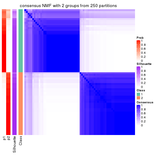
consensus_heatmap(res, k = 3)
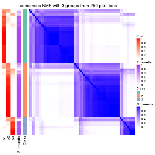
consensus_heatmap(res, k = 4)
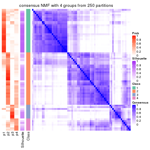
consensus_heatmap(res, k = 5)
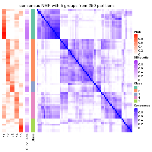
consensus_heatmap(res, k = 6)
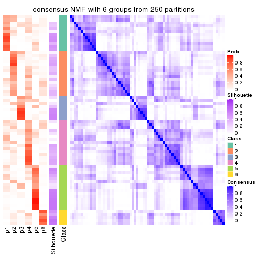
Heatmaps for the membership of samples in all partitions to see how consistent they are:
membership_heatmap(res, k = 2)
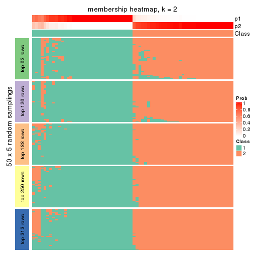
membership_heatmap(res, k = 3)
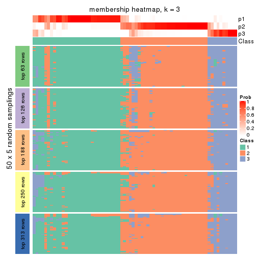
membership_heatmap(res, k = 4)
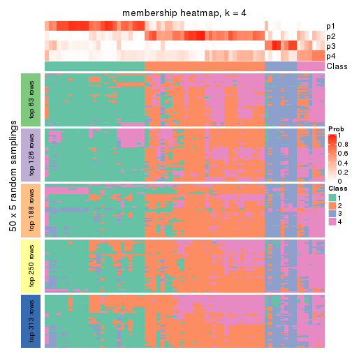
membership_heatmap(res, k = 5)
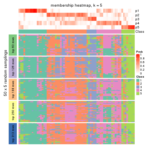
membership_heatmap(res, k = 6)
As soon as we have had the classes for columns, we can look for signatures which are significantly different between classes which can be candidate marks for certain classes. Following are the heatmaps for signatures.
Signature heatmaps where rows are scaled:
get_signatures(res, k = 2)
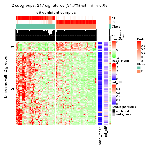
get_signatures(res, k = 3)
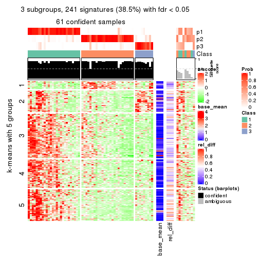
get_signatures(res, k = 4)
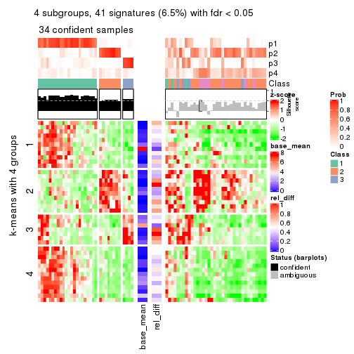
get_signatures(res, k = 5)
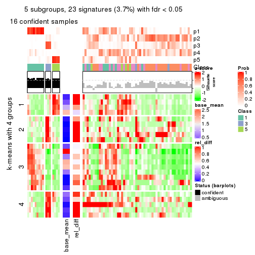
get_signatures(res, k = 6)
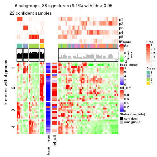
Signature heatmaps where rows are not scaled:
get_signatures(res, k = 2, scale_rows = FALSE)
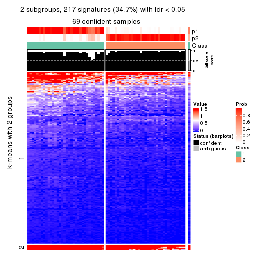
get_signatures(res, k = 3, scale_rows = FALSE)
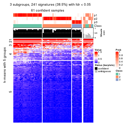
get_signatures(res, k = 4, scale_rows = FALSE)
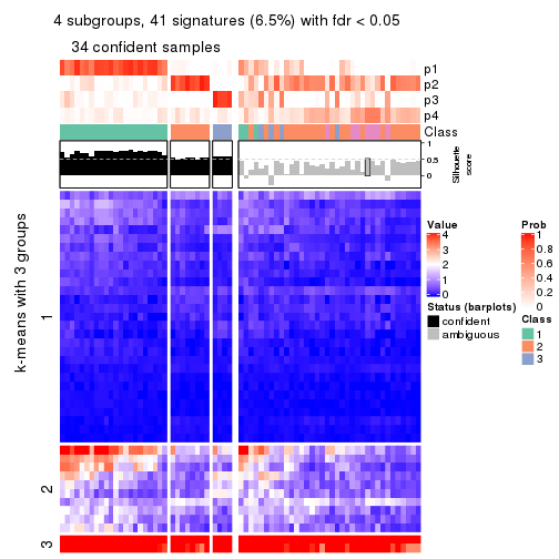
get_signatures(res, k = 5, scale_rows = FALSE)
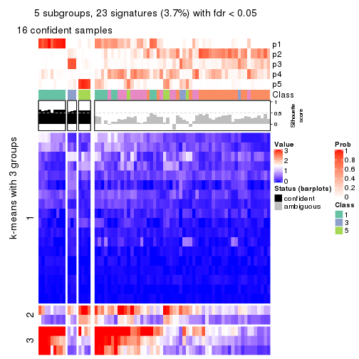
get_signatures(res, k = 6, scale_rows = FALSE)
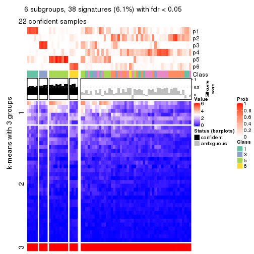
Compare the overlap of signatures from different k:
compare_signatures(res)
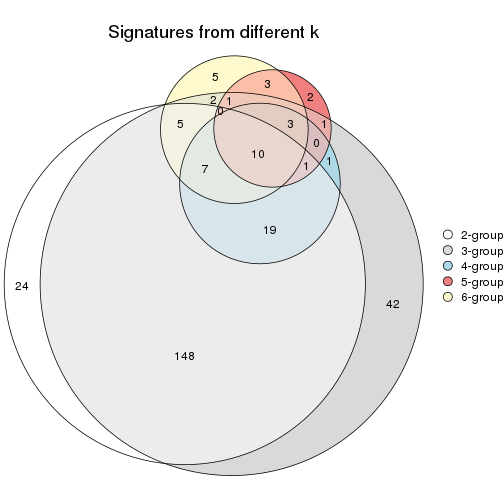
get_signature() returns a data frame invisibly. TO get the list of signatures, the function
call should be assigned to a variable explicitly. In following code, if plot argument is set
to FALSE, no heatmap is plotted while only the differential analysis is performed.
# code only for demonstration
tb = get_signature(res, k = ..., plot = FALSE)
An example of the output of tb is:
#> which_row fdr mean_1 mean_2 scaled_mean_1 scaled_mean_2 km
#> 1 38 0.042760348 8.373488 9.131774 -0.5533452 0.5164555 1
#> 2 40 0.018707592 7.106213 8.469186 -0.6173731 0.5762149 1
#> 3 55 0.019134737 10.221463 11.207825 -0.6159697 0.5749050 1
#> 4 59 0.006059896 5.921854 7.869574 -0.6899429 0.6439467 1
#> 5 60 0.018055526 8.928898 10.211722 -0.6204761 0.5791110 1
#> 6 98 0.009384629 15.714769 14.887706 0.6635654 -0.6193277 2
...
The columns in tb are:
which_row: row indices corresponding to the input matrix.fdr: FDR for the differential test. mean_x: The mean value in group x.scaled_mean_x: The mean value in group x after rows are scaled.km: Row groups if k-means clustering is applied to rows.UMAP plot which shows how samples are separated.
dimension_reduction(res, k = 2, method = "UMAP")
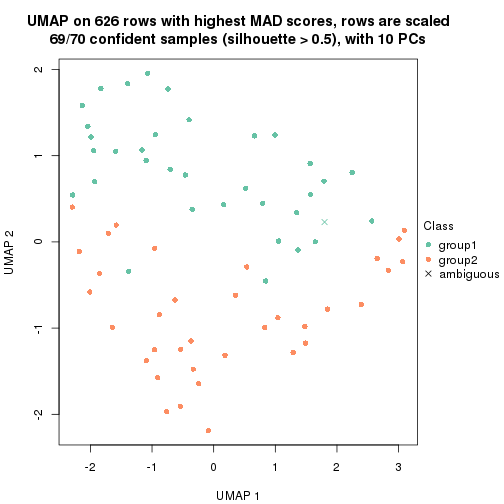
dimension_reduction(res, k = 3, method = "UMAP")
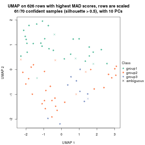
dimension_reduction(res, k = 4, method = "UMAP")
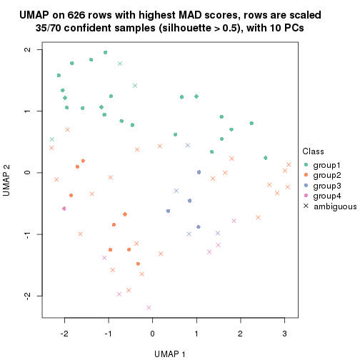
dimension_reduction(res, k = 5, method = "UMAP")
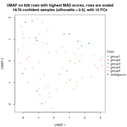
dimension_reduction(res, k = 6, method = "UMAP")
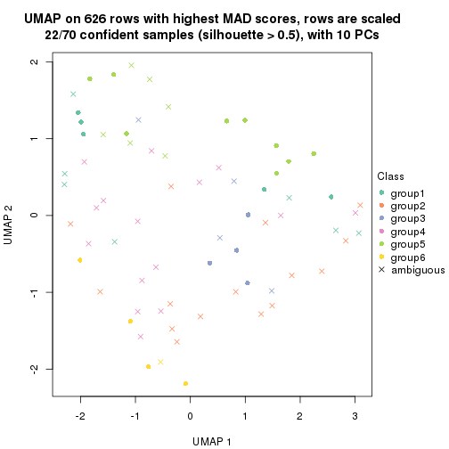
Following heatmap shows how subgroups are split when increasing k:
collect_classes(res)
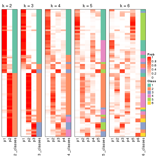
If matrix rows can be associated to genes, consider to use functional_enrichment(res,
...) to perform function enrichment for the signature genes. See this vignette for more detailed explanations.
The object with results only for a single top-value method and a single partition method can be extracted as:
res = res_list["ATC", "hclust"]
# you can also extract it by
# res = res_list["ATC:hclust"]
A summary of res and all the functions that can be applied to it:
res
#> A 'ConsensusPartition' object with k = 2, 3, 4, 5, 6.
#> On a matrix with 626 rows and 70 columns.
#> Top rows (63, 126, 188, 250, 313) are extracted by 'ATC' method.
#> Subgroups are detected by 'hclust' method.
#> Performed in total 1250 partitions by row resampling.
#> Best k for subgroups seems to be 3.
#>
#> Following methods can be applied to this 'ConsensusPartition' object:
#> [1] "cola_report" "collect_classes" "collect_plots"
#> [4] "collect_stats" "colnames" "compare_signatures"
#> [7] "consensus_heatmap" "dimension_reduction" "functional_enrichment"
#> [10] "get_anno_col" "get_anno" "get_classes"
#> [13] "get_consensus" "get_matrix" "get_membership"
#> [16] "get_param" "get_signatures" "get_stats"
#> [19] "is_best_k" "is_stable_k" "membership_heatmap"
#> [22] "ncol" "nrow" "plot_ecdf"
#> [25] "rownames" "select_partition_number" "show"
#> [28] "suggest_best_k" "test_to_known_factors"
collect_plots() function collects all the plots made from res for all k (number of partitions)
into one single page to provide an easy and fast comparison between different k.
collect_plots(res)
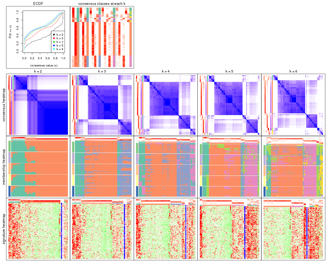
The plots are:
k and the heatmap of
predicted classes for each k.k.k.k.All the plots in panels can be made by individual functions and they are plotted later in this section.
select_partition_number() produces several plots showing different
statistics for choosing “optimized” k. There are following statistics:
k;k, the area increased is defined as \(A_k - A_{k-1}\).The detailed explanations of these statistics can be found in the cola vignette.
Generally speaking, lower PAC score, higher mean silhouette score or higher
concordance corresponds to better partition. Rand index and Jaccard index
measure how similar the current partition is compared to partition with k-1.
If they are too similar, we won't accept k is better than k-1.
select_partition_number(res)
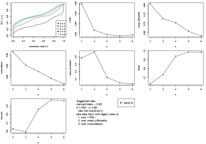
The numeric values for all these statistics can be obtained by get_stats().
get_stats(res)
#> k 1-PAC mean_silhouette concordance area_increased Rand Jaccard
#> 2 2 0.597 0.807 0.914 0.3860 0.627 0.627
#> 3 3 0.469 0.728 0.853 0.4659 0.733 0.592
#> 4 4 0.447 0.705 0.824 0.1207 0.941 0.861
#> 5 5 0.441 0.658 0.792 0.0481 0.989 0.972
#> 6 6 0.446 0.633 0.767 0.0325 0.986 0.964
suggest_best_k() suggests the best \(k\) based on these statistics. The rules are as follows:
suggest_best_k(res)
#> [1] 3
Following shows the table of the partitions (You need to click the show/hide
code output link to see it). The membership matrix (columns with name p*)
is inferred by
clue::cl_consensus()
function with the SE method. Basically the value in the membership matrix
represents the probability to belong to a certain group. The finall class
label for an item is determined with the group with highest probability it
belongs to.
In get_classes() function, the entropy is calculated from the membership
matrix and the silhouette score is calculated from the consensus matrix.
cbind(get_classes(res, k = 2), get_membership(res, k = 2))
#> class entropy silhouette p1 p2
#> SRR837437 2 0.0000 0.904 0.000 1.000
#> SRR837438 2 0.9358 0.490 0.352 0.648
#> SRR837439 2 0.1414 0.896 0.020 0.980
#> SRR837440 2 0.0672 0.901 0.008 0.992
#> SRR837441 2 0.1414 0.896 0.020 0.980
#> SRR837442 2 0.0000 0.904 0.000 1.000
#> SRR837443 2 0.0000 0.904 0.000 1.000
#> SRR837444 2 0.7674 0.712 0.224 0.776
#> SRR837445 2 0.7528 0.720 0.216 0.784
#> SRR837446 2 0.0000 0.904 0.000 1.000
#> SRR837447 1 0.0000 0.870 1.000 0.000
#> SRR837448 1 0.0000 0.870 1.000 0.000
#> SRR837449 1 0.1843 0.875 0.972 0.028
#> SRR837450 1 0.3879 0.866 0.924 0.076
#> SRR837451 2 0.0000 0.904 0.000 1.000
#> SRR837452 2 0.1633 0.893 0.024 0.976
#> SRR837453 2 0.0000 0.904 0.000 1.000
#> SRR837454 2 0.0000 0.904 0.000 1.000
#> SRR837455 1 0.0000 0.870 1.000 0.000
#> SRR837456 1 0.0000 0.870 1.000 0.000
#> SRR837457 2 0.0000 0.904 0.000 1.000
#> SRR837458 1 0.0000 0.870 1.000 0.000
#> SRR837459 2 0.0000 0.904 0.000 1.000
#> SRR837460 2 0.0000 0.904 0.000 1.000
#> SRR837461 2 0.0000 0.904 0.000 1.000
#> SRR837462 2 0.8813 0.595 0.300 0.700
#> SRR837463 2 0.9170 0.534 0.332 0.668
#> SRR837464 2 0.1633 0.894 0.024 0.976
#> SRR837465 2 0.8763 0.602 0.296 0.704
#> SRR837466 1 0.0000 0.870 1.000 0.000
#> SRR837467 2 0.0000 0.904 0.000 1.000
#> SRR837468 2 0.2043 0.889 0.032 0.968
#> SRR837469 1 0.2236 0.876 0.964 0.036
#> SRR837470 1 0.2236 0.876 0.964 0.036
#> SRR837471 2 0.5059 0.827 0.112 0.888
#> SRR837472 2 0.2043 0.888 0.032 0.968
#> SRR837473 2 0.9815 0.305 0.420 0.580
#> SRR837474 2 0.0000 0.904 0.000 1.000
#> SRR837475 2 0.0000 0.904 0.000 1.000
#> SRR837476 2 0.0000 0.904 0.000 1.000
#> SRR837477 2 0.8207 0.669 0.256 0.744
#> SRR837478 2 0.0000 0.904 0.000 1.000
#> SRR837479 2 0.0000 0.904 0.000 1.000
#> SRR837480 2 0.0000 0.904 0.000 1.000
#> SRR837481 2 0.0000 0.904 0.000 1.000
#> SRR837482 2 0.0672 0.901 0.008 0.992
#> SRR837483 1 0.4161 0.863 0.916 0.084
#> SRR837484 2 0.0000 0.904 0.000 1.000
#> SRR837485 2 0.0000 0.904 0.000 1.000
#> SRR837486 2 0.1184 0.898 0.016 0.984
#> SRR837487 2 0.0000 0.904 0.000 1.000
#> SRR837488 2 0.0000 0.904 0.000 1.000
#> SRR837489 2 0.0000 0.904 0.000 1.000
#> SRR837490 2 0.0000 0.904 0.000 1.000
#> SRR837491 2 0.8207 0.668 0.256 0.744
#> SRR837492 2 0.8763 0.605 0.296 0.704
#> SRR837493 2 0.9323 0.500 0.348 0.652
#> SRR837494 2 0.0000 0.904 0.000 1.000
#> SRR837495 2 0.7056 0.747 0.192 0.808
#> SRR837496 1 0.6438 0.802 0.836 0.164
#> SRR837497 1 0.6887 0.777 0.816 0.184
#> SRR837498 1 0.4431 0.858 0.908 0.092
#> SRR837499 1 0.9909 0.182 0.556 0.444
#> SRR837500 1 0.9922 0.167 0.552 0.448
#> SRR837501 2 0.0000 0.904 0.000 1.000
#> SRR837502 2 0.9933 0.194 0.452 0.548
#> SRR837503 1 0.6531 0.798 0.832 0.168
#> SRR837504 2 0.0000 0.904 0.000 1.000
#> SRR837505 2 0.0000 0.904 0.000 1.000
#> SRR837506 2 0.0000 0.904 0.000 1.000
cbind(get_classes(res, k = 3), get_membership(res, k = 3))
#> class entropy silhouette p1 p2 p3
#> SRR837437 2 0.0424 0.896 0.000 0.992 0.008
#> SRR837438 3 0.4002 0.714 0.000 0.160 0.840
#> SRR837439 2 0.3879 0.819 0.000 0.848 0.152
#> SRR837440 2 0.2448 0.881 0.000 0.924 0.076
#> SRR837441 2 0.3879 0.819 0.000 0.848 0.152
#> SRR837442 2 0.0892 0.897 0.000 0.980 0.020
#> SRR837443 2 0.1031 0.897 0.000 0.976 0.024
#> SRR837444 3 0.5678 0.632 0.000 0.316 0.684
#> SRR837445 3 0.5733 0.621 0.000 0.324 0.676
#> SRR837446 2 0.1643 0.896 0.000 0.956 0.044
#> SRR837447 1 0.1964 0.820 0.944 0.000 0.056
#> SRR837448 1 0.0892 0.805 0.980 0.000 0.020
#> SRR837449 1 0.4235 0.795 0.824 0.000 0.176
#> SRR837450 1 0.5465 0.727 0.712 0.000 0.288
#> SRR837451 2 0.0424 0.892 0.000 0.992 0.008
#> SRR837452 2 0.2625 0.876 0.000 0.916 0.084
#> SRR837453 2 0.0424 0.892 0.000 0.992 0.008
#> SRR837454 2 0.0237 0.893 0.000 0.996 0.004
#> SRR837455 1 0.1753 0.820 0.952 0.000 0.048
#> SRR837456 1 0.1753 0.820 0.952 0.000 0.048
#> SRR837457 2 0.0424 0.892 0.000 0.992 0.008
#> SRR837458 1 0.0892 0.805 0.980 0.000 0.020
#> SRR837459 2 0.0424 0.892 0.000 0.992 0.008
#> SRR837460 2 0.0424 0.892 0.000 0.992 0.008
#> SRR837461 2 0.1163 0.897 0.000 0.972 0.028
#> SRR837462 3 0.4974 0.722 0.000 0.236 0.764
#> SRR837463 3 0.4452 0.724 0.000 0.192 0.808
#> SRR837464 2 0.5291 0.649 0.000 0.732 0.268
#> SRR837465 3 0.5016 0.721 0.000 0.240 0.760
#> SRR837466 1 0.0892 0.805 0.980 0.000 0.020
#> SRR837467 2 0.0592 0.896 0.000 0.988 0.012
#> SRR837468 2 0.5465 0.615 0.000 0.712 0.288
#> SRR837469 1 0.5706 0.703 0.680 0.000 0.320
#> SRR837470 1 0.5591 0.718 0.696 0.000 0.304
#> SRR837471 2 0.6291 -0.033 0.000 0.532 0.468
#> SRR837472 2 0.4931 0.707 0.000 0.768 0.232
#> SRR837473 3 0.3846 0.671 0.016 0.108 0.876
#> SRR837474 2 0.3267 0.853 0.000 0.884 0.116
#> SRR837475 2 0.3340 0.849 0.000 0.880 0.120
#> SRR837476 2 0.2448 0.880 0.000 0.924 0.076
#> SRR837477 3 0.5465 0.670 0.000 0.288 0.712
#> SRR837478 2 0.2165 0.885 0.000 0.936 0.064
#> SRR837479 2 0.4002 0.821 0.000 0.840 0.160
#> SRR837480 2 0.3816 0.824 0.000 0.852 0.148
#> SRR837481 2 0.3879 0.821 0.000 0.848 0.152
#> SRR837482 2 0.4555 0.764 0.000 0.800 0.200
#> SRR837483 1 0.6359 0.603 0.592 0.004 0.404
#> SRR837484 2 0.0892 0.897 0.000 0.980 0.020
#> SRR837485 2 0.1163 0.897 0.000 0.972 0.028
#> SRR837486 2 0.4974 0.715 0.000 0.764 0.236
#> SRR837487 2 0.0592 0.897 0.000 0.988 0.012
#> SRR837488 2 0.0424 0.892 0.000 0.992 0.008
#> SRR837489 2 0.2356 0.883 0.000 0.928 0.072
#> SRR837490 2 0.2261 0.885 0.000 0.932 0.068
#> SRR837491 3 0.5591 0.660 0.000 0.304 0.696
#> SRR837492 3 0.5201 0.719 0.004 0.236 0.760
#> SRR837493 3 0.4121 0.718 0.000 0.168 0.832
#> SRR837494 2 0.0237 0.893 0.000 0.996 0.004
#> SRR837495 3 0.6062 0.488 0.000 0.384 0.616
#> SRR837496 3 0.6225 -0.352 0.432 0.000 0.568
#> SRR837497 3 0.6095 -0.257 0.392 0.000 0.608
#> SRR837498 1 0.6302 0.472 0.520 0.000 0.480
#> SRR837499 3 0.3722 0.503 0.088 0.024 0.888
#> SRR837500 3 0.3765 0.511 0.084 0.028 0.888
#> SRR837501 2 0.0892 0.897 0.000 0.980 0.020
#> SRR837502 3 0.3415 0.639 0.020 0.080 0.900
#> SRR837503 3 0.6244 -0.356 0.440 0.000 0.560
#> SRR837504 2 0.0747 0.896 0.000 0.984 0.016
#> SRR837505 2 0.2356 0.886 0.000 0.928 0.072
#> SRR837506 2 0.0424 0.892 0.000 0.992 0.008
cbind(get_classes(res, k = 4), get_membership(res, k = 4))
#> class entropy silhouette p1 p2 p3 p4
#> SRR837437 2 0.0804 0.864 0.000 0.980 0.012 0.008
#> SRR837438 3 0.1936 0.761 0.000 0.028 0.940 0.032
#> SRR837439 2 0.3649 0.780 0.000 0.796 0.204 0.000
#> SRR837440 2 0.2530 0.850 0.000 0.888 0.112 0.000
#> SRR837441 2 0.3649 0.780 0.000 0.796 0.204 0.000
#> SRR837442 2 0.1209 0.868 0.000 0.964 0.032 0.004
#> SRR837443 2 0.1557 0.865 0.000 0.944 0.056 0.000
#> SRR837444 3 0.3355 0.760 0.000 0.160 0.836 0.004
#> SRR837445 3 0.3266 0.757 0.000 0.168 0.832 0.000
#> SRR837446 2 0.1792 0.867 0.000 0.932 0.068 0.000
#> SRR837447 1 0.4543 0.609 0.676 0.000 0.000 0.324
#> SRR837448 1 0.0336 0.623 0.992 0.000 0.000 0.008
#> SRR837449 1 0.5842 0.349 0.520 0.000 0.032 0.448
#> SRR837450 1 0.6633 -0.238 0.500 0.000 0.084 0.416
#> SRR837451 2 0.1356 0.854 0.000 0.960 0.008 0.032
#> SRR837452 2 0.2704 0.846 0.000 0.876 0.124 0.000
#> SRR837453 2 0.1356 0.854 0.000 0.960 0.008 0.032
#> SRR837454 2 0.0657 0.861 0.000 0.984 0.004 0.012
#> SRR837455 1 0.4406 0.627 0.700 0.000 0.000 0.300
#> SRR837456 1 0.4406 0.627 0.700 0.000 0.000 0.300
#> SRR837457 2 0.1356 0.854 0.000 0.960 0.008 0.032
#> SRR837458 1 0.0000 0.624 1.000 0.000 0.000 0.000
#> SRR837459 2 0.1356 0.854 0.000 0.960 0.008 0.032
#> SRR837460 2 0.1356 0.854 0.000 0.960 0.008 0.032
#> SRR837461 2 0.1824 0.867 0.000 0.936 0.060 0.004
#> SRR837462 3 0.3205 0.787 0.000 0.104 0.872 0.024
#> SRR837463 3 0.2197 0.773 0.000 0.048 0.928 0.024
#> SRR837464 2 0.5004 0.453 0.000 0.604 0.392 0.004
#> SRR837465 3 0.3099 0.787 0.000 0.104 0.876 0.020
#> SRR837466 1 0.0336 0.623 0.992 0.000 0.000 0.008
#> SRR837467 2 0.0592 0.865 0.000 0.984 0.016 0.000
#> SRR837468 2 0.5050 0.422 0.000 0.588 0.408 0.004
#> SRR837469 4 0.5498 0.321 0.272 0.000 0.048 0.680
#> SRR837470 4 0.5972 0.277 0.304 0.000 0.064 0.632
#> SRR837471 3 0.4843 0.323 0.000 0.396 0.604 0.000
#> SRR837472 2 0.4543 0.612 0.000 0.676 0.324 0.000
#> SRR837473 3 0.3443 0.685 0.000 0.016 0.848 0.136
#> SRR837474 2 0.3400 0.805 0.000 0.820 0.180 0.000
#> SRR837475 2 0.3444 0.800 0.000 0.816 0.184 0.000
#> SRR837476 2 0.2814 0.841 0.000 0.868 0.132 0.000
#> SRR837477 3 0.3271 0.771 0.000 0.132 0.856 0.012
#> SRR837478 2 0.2334 0.855 0.000 0.908 0.088 0.004
#> SRR837479 2 0.4872 0.733 0.000 0.728 0.244 0.028
#> SRR837480 2 0.4008 0.736 0.000 0.756 0.244 0.000
#> SRR837481 2 0.4072 0.729 0.000 0.748 0.252 0.000
#> SRR837482 2 0.4655 0.638 0.000 0.684 0.312 0.004
#> SRR837483 4 0.6529 0.242 0.388 0.000 0.080 0.532
#> SRR837484 2 0.1398 0.867 0.000 0.956 0.040 0.004
#> SRR837485 2 0.1661 0.866 0.000 0.944 0.052 0.004
#> SRR837486 2 0.4679 0.576 0.000 0.648 0.352 0.000
#> SRR837487 2 0.1209 0.867 0.000 0.964 0.032 0.004
#> SRR837488 2 0.1356 0.854 0.000 0.960 0.008 0.032
#> SRR837489 2 0.2704 0.844 0.000 0.876 0.124 0.000
#> SRR837490 2 0.2647 0.846 0.000 0.880 0.120 0.000
#> SRR837491 3 0.3401 0.770 0.000 0.152 0.840 0.008
#> SRR837492 3 0.3051 0.784 0.000 0.088 0.884 0.028
#> SRR837493 3 0.1733 0.766 0.000 0.028 0.948 0.024
#> SRR837494 2 0.0779 0.859 0.000 0.980 0.004 0.016
#> SRR837495 3 0.3873 0.693 0.000 0.228 0.772 0.000
#> SRR837496 4 0.6664 0.593 0.164 0.000 0.216 0.620
#> SRR837497 4 0.6209 0.597 0.112 0.000 0.232 0.656
#> SRR837498 4 0.5321 0.556 0.140 0.000 0.112 0.748
#> SRR837499 3 0.4853 0.496 0.036 0.000 0.744 0.220
#> SRR837500 3 0.4764 0.500 0.032 0.000 0.748 0.220
#> SRR837501 2 0.1388 0.869 0.000 0.960 0.028 0.012
#> SRR837502 3 0.2888 0.674 0.000 0.004 0.872 0.124
#> SRR837503 4 0.6646 0.593 0.156 0.000 0.224 0.620
#> SRR837504 2 0.0895 0.865 0.000 0.976 0.020 0.004
#> SRR837505 2 0.3598 0.840 0.000 0.848 0.124 0.028
#> SRR837506 2 0.1356 0.854 0.000 0.960 0.008 0.032
cbind(get_classes(res, k = 5), get_membership(res, k = 5))
#> class entropy silhouette p1 p2 p3 p4 p5
#> SRR837437 2 0.1281 0.837 0.000 0.956 0.000 0.012 0.032
#> SRR837438 4 0.1419 0.775 0.000 0.016 0.012 0.956 0.016
#> SRR837439 2 0.3779 0.754 0.000 0.776 0.000 0.200 0.024
#> SRR837440 2 0.2813 0.821 0.000 0.868 0.000 0.108 0.024
#> SRR837441 2 0.3779 0.754 0.000 0.776 0.000 0.200 0.024
#> SRR837442 2 0.1386 0.842 0.000 0.952 0.000 0.032 0.016
#> SRR837443 2 0.1697 0.838 0.000 0.932 0.000 0.060 0.008
#> SRR837444 4 0.3484 0.763 0.000 0.144 0.004 0.824 0.028
#> SRR837445 4 0.3531 0.766 0.000 0.148 0.000 0.816 0.036
#> SRR837446 2 0.1942 0.841 0.000 0.920 0.000 0.068 0.012
#> SRR837447 1 0.1478 0.559 0.936 0.000 0.064 0.000 0.000
#> SRR837448 1 0.4341 0.369 0.592 0.000 0.004 0.000 0.404
#> SRR837449 1 0.4370 0.347 0.744 0.000 0.200 0.000 0.056
#> SRR837450 5 0.6848 0.333 0.232 0.000 0.316 0.008 0.444
#> SRR837451 2 0.2020 0.815 0.000 0.900 0.000 0.000 0.100
#> SRR837452 2 0.2773 0.828 0.000 0.868 0.000 0.112 0.020
#> SRR837453 2 0.2020 0.815 0.000 0.900 0.000 0.000 0.100
#> SRR837454 2 0.1357 0.833 0.000 0.948 0.000 0.004 0.048
#> SRR837455 1 0.0000 0.580 1.000 0.000 0.000 0.000 0.000
#> SRR837456 1 0.0000 0.580 1.000 0.000 0.000 0.000 0.000
#> SRR837457 2 0.2020 0.815 0.000 0.900 0.000 0.000 0.100
#> SRR837458 1 0.4310 0.379 0.604 0.000 0.004 0.000 0.392
#> SRR837459 2 0.2020 0.815 0.000 0.900 0.000 0.000 0.100
#> SRR837460 2 0.2020 0.815 0.000 0.900 0.000 0.000 0.100
#> SRR837461 2 0.2124 0.841 0.000 0.916 0.000 0.056 0.028
#> SRR837462 4 0.2701 0.794 0.000 0.092 0.012 0.884 0.012
#> SRR837463 4 0.1854 0.786 0.000 0.036 0.008 0.936 0.020
#> SRR837464 2 0.5672 0.361 0.000 0.544 0.000 0.368 0.088
#> SRR837465 4 0.2589 0.794 0.000 0.092 0.012 0.888 0.008
#> SRR837466 1 0.4341 0.369 0.592 0.000 0.004 0.000 0.404
#> SRR837467 2 0.0912 0.838 0.000 0.972 0.000 0.016 0.012
#> SRR837468 2 0.5663 0.338 0.000 0.532 0.000 0.384 0.084
#> SRR837469 3 0.4670 0.219 0.440 0.000 0.548 0.004 0.008
#> SRR837470 1 0.5731 -0.366 0.480 0.000 0.456 0.016 0.048
#> SRR837471 4 0.5143 0.368 0.000 0.368 0.000 0.584 0.048
#> SRR837472 2 0.4902 0.577 0.000 0.648 0.000 0.304 0.048
#> SRR837473 4 0.3715 0.695 0.000 0.004 0.064 0.824 0.108
#> SRR837474 2 0.3574 0.779 0.000 0.804 0.000 0.168 0.028
#> SRR837475 2 0.3612 0.774 0.000 0.800 0.000 0.172 0.028
#> SRR837476 2 0.3106 0.812 0.000 0.844 0.000 0.132 0.024
#> SRR837477 4 0.4079 0.771 0.000 0.108 0.008 0.804 0.080
#> SRR837478 2 0.2448 0.832 0.000 0.892 0.000 0.088 0.020
#> SRR837479 2 0.5312 0.689 0.000 0.664 0.000 0.220 0.116
#> SRR837480 2 0.4766 0.686 0.000 0.708 0.000 0.220 0.072
#> SRR837481 2 0.4765 0.677 0.000 0.704 0.000 0.228 0.068
#> SRR837482 2 0.5353 0.582 0.000 0.636 0.000 0.272 0.092
#> SRR837483 5 0.4410 0.413 0.008 0.000 0.276 0.016 0.700
#> SRR837484 2 0.1568 0.841 0.000 0.944 0.000 0.036 0.020
#> SRR837485 2 0.1893 0.842 0.000 0.928 0.000 0.048 0.024
#> SRR837486 2 0.5300 0.513 0.000 0.604 0.000 0.328 0.068
#> SRR837487 2 0.1399 0.841 0.000 0.952 0.000 0.028 0.020
#> SRR837488 2 0.2020 0.815 0.000 0.900 0.000 0.000 0.100
#> SRR837489 2 0.2563 0.820 0.000 0.872 0.000 0.120 0.008
#> SRR837490 2 0.2513 0.822 0.000 0.876 0.000 0.116 0.008
#> SRR837491 4 0.3460 0.779 0.000 0.128 0.000 0.828 0.044
#> SRR837492 4 0.3765 0.783 0.000 0.064 0.020 0.836 0.080
#> SRR837493 4 0.1710 0.781 0.000 0.020 0.012 0.944 0.024
#> SRR837494 2 0.1544 0.826 0.000 0.932 0.000 0.000 0.068
#> SRR837495 4 0.4392 0.708 0.000 0.200 0.004 0.748 0.048
#> SRR837496 3 0.7018 0.145 0.124 0.000 0.528 0.064 0.284
#> SRR837497 3 0.3340 0.368 0.064 0.000 0.864 0.048 0.024
#> SRR837498 3 0.5592 0.418 0.252 0.000 0.656 0.028 0.064
#> SRR837499 4 0.5339 0.559 0.040 0.000 0.148 0.724 0.088
#> SRR837500 4 0.5304 0.562 0.036 0.000 0.152 0.724 0.088
#> SRR837501 2 0.2006 0.840 0.000 0.916 0.000 0.012 0.072
#> SRR837502 4 0.2927 0.708 0.000 0.000 0.092 0.868 0.040
#> SRR837503 3 0.6889 0.170 0.112 0.000 0.544 0.064 0.280
#> SRR837504 2 0.1310 0.840 0.000 0.956 0.000 0.024 0.020
#> SRR837505 2 0.4219 0.798 0.000 0.780 0.000 0.104 0.116
#> SRR837506 2 0.2358 0.810 0.000 0.888 0.008 0.000 0.104
cbind(get_classes(res, k = 6), get_membership(res, k = 6))
#> class entropy silhouette p1 p2 p3 p4 p5 p6
#> SRR837437 2 0.1219 0.8133 0.048 0.948 0.000 0.004 0.000 0.000
#> SRR837438 4 0.1129 0.7693 0.004 0.012 0.012 0.964 0.000 0.008
#> SRR837439 2 0.3822 0.7343 0.032 0.772 0.016 0.180 0.000 0.000
#> SRR837440 2 0.2863 0.7983 0.036 0.860 0.008 0.096 0.000 0.000
#> SRR837441 2 0.3822 0.7343 0.032 0.772 0.016 0.180 0.000 0.000
#> SRR837442 2 0.1341 0.8170 0.024 0.948 0.000 0.028 0.000 0.000
#> SRR837443 2 0.1528 0.8143 0.016 0.936 0.000 0.048 0.000 0.000
#> SRR837444 4 0.3412 0.7460 0.032 0.144 0.012 0.812 0.000 0.000
#> SRR837445 4 0.3624 0.7553 0.036 0.144 0.012 0.804 0.000 0.004
#> SRR837446 2 0.2076 0.8175 0.016 0.912 0.012 0.060 0.000 0.000
#> SRR837447 1 0.4937 0.4654 0.548 0.000 0.020 0.000 0.400 0.032
#> SRR837448 5 0.0146 0.9780 0.000 0.000 0.000 0.000 0.996 0.004
#> SRR837449 1 0.6513 0.4552 0.480 0.000 0.044 0.000 0.276 0.200
#> SRR837450 6 0.6329 0.2916 0.064 0.000 0.104 0.004 0.304 0.524
#> SRR837451 2 0.2003 0.7917 0.116 0.884 0.000 0.000 0.000 0.000
#> SRR837452 2 0.2653 0.8048 0.028 0.868 0.004 0.100 0.000 0.000
#> SRR837453 2 0.2003 0.7917 0.116 0.884 0.000 0.000 0.000 0.000
#> SRR837454 2 0.1285 0.8104 0.052 0.944 0.000 0.004 0.000 0.000
#> SRR837455 1 0.3868 0.3711 0.508 0.000 0.000 0.000 0.492 0.000
#> SRR837456 1 0.3868 0.3711 0.508 0.000 0.000 0.000 0.492 0.000
#> SRR837457 2 0.2003 0.7917 0.116 0.884 0.000 0.000 0.000 0.000
#> SRR837458 5 0.0984 0.9554 0.012 0.000 0.008 0.000 0.968 0.012
#> SRR837459 2 0.2003 0.7917 0.116 0.884 0.000 0.000 0.000 0.000
#> SRR837460 2 0.2003 0.7917 0.116 0.884 0.000 0.000 0.000 0.000
#> SRR837461 2 0.2426 0.8168 0.048 0.896 0.012 0.044 0.000 0.000
#> SRR837462 4 0.2405 0.7827 0.008 0.080 0.016 0.892 0.000 0.004
#> SRR837463 4 0.1686 0.7762 0.016 0.024 0.016 0.940 0.000 0.004
#> SRR837464 2 0.6514 0.2079 0.152 0.448 0.052 0.348 0.000 0.000
#> SRR837465 4 0.2262 0.7830 0.008 0.080 0.016 0.896 0.000 0.000
#> SRR837466 5 0.0146 0.9780 0.000 0.000 0.000 0.000 0.996 0.004
#> SRR837467 2 0.0909 0.8163 0.020 0.968 0.000 0.012 0.000 0.000
#> SRR837468 2 0.6533 0.1727 0.152 0.432 0.052 0.364 0.000 0.000
#> SRR837469 1 0.7006 -0.1544 0.376 0.000 0.356 0.004 0.064 0.200
#> SRR837470 1 0.7529 -0.0487 0.364 0.000 0.236 0.016 0.088 0.296
#> SRR837471 4 0.5273 0.3675 0.076 0.360 0.012 0.552 0.000 0.000
#> SRR837472 2 0.4979 0.5530 0.076 0.636 0.012 0.276 0.000 0.000
#> SRR837473 4 0.3798 0.6803 0.060 0.000 0.040 0.812 0.000 0.088
#> SRR837474 2 0.3473 0.7588 0.048 0.804 0.004 0.144 0.000 0.000
#> SRR837475 2 0.3511 0.7540 0.048 0.800 0.004 0.148 0.000 0.000
#> SRR837476 2 0.3076 0.7899 0.044 0.840 0.004 0.112 0.000 0.000
#> SRR837477 4 0.4498 0.7540 0.088 0.092 0.036 0.772 0.000 0.012
#> SRR837478 2 0.2728 0.8099 0.040 0.872 0.008 0.080 0.000 0.000
#> SRR837479 2 0.5786 0.6210 0.180 0.596 0.028 0.196 0.000 0.000
#> SRR837480 2 0.5464 0.6161 0.144 0.640 0.028 0.188 0.000 0.000
#> SRR837481 2 0.5654 0.5994 0.136 0.632 0.032 0.196 0.000 0.004
#> SRR837482 2 0.6375 0.4533 0.168 0.532 0.044 0.252 0.000 0.004
#> SRR837483 6 0.6994 0.1921 0.060 0.000 0.300 0.000 0.276 0.364
#> SRR837484 2 0.1716 0.8180 0.036 0.932 0.004 0.028 0.000 0.000
#> SRR837485 2 0.2138 0.8176 0.052 0.908 0.004 0.036 0.000 0.000
#> SRR837486 2 0.6095 0.4176 0.132 0.532 0.040 0.296 0.000 0.000
#> SRR837487 2 0.1552 0.8177 0.036 0.940 0.004 0.020 0.000 0.000
#> SRR837488 2 0.2003 0.7917 0.116 0.884 0.000 0.000 0.000 0.000
#> SRR837489 2 0.2455 0.7979 0.012 0.872 0.004 0.112 0.000 0.000
#> SRR837490 2 0.2408 0.7999 0.012 0.876 0.004 0.108 0.000 0.000
#> SRR837491 4 0.3674 0.7713 0.060 0.104 0.016 0.816 0.000 0.004
#> SRR837492 4 0.4104 0.7646 0.084 0.048 0.036 0.808 0.000 0.024
#> SRR837493 4 0.1425 0.7778 0.012 0.020 0.008 0.952 0.000 0.008
#> SRR837494 2 0.1556 0.8033 0.080 0.920 0.000 0.000 0.000 0.000
#> SRR837495 4 0.4569 0.6957 0.052 0.196 0.024 0.724 0.000 0.004
#> SRR837496 6 0.2940 0.2489 0.012 0.000 0.016 0.048 0.048 0.876
#> SRR837497 3 0.4852 0.0000 0.016 0.000 0.604 0.012 0.020 0.348
#> SRR837498 6 0.6662 -0.4828 0.232 0.000 0.360 0.012 0.016 0.380
#> SRR837499 4 0.4405 0.5684 0.028 0.000 0.040 0.724 0.000 0.208
#> SRR837500 4 0.4441 0.5715 0.028 0.000 0.044 0.724 0.000 0.204
#> SRR837501 2 0.3473 0.7804 0.144 0.804 0.048 0.004 0.000 0.000
#> SRR837502 4 0.2853 0.7025 0.012 0.000 0.048 0.868 0.000 0.072
#> SRR837503 6 0.3398 0.2223 0.008 0.000 0.032 0.044 0.068 0.848
#> SRR837504 2 0.1092 0.8163 0.020 0.960 0.000 0.020 0.000 0.000
#> SRR837505 2 0.4672 0.7475 0.176 0.716 0.020 0.088 0.000 0.000
#> SRR837506 2 0.3973 0.7391 0.140 0.784 0.048 0.000 0.000 0.028
Heatmaps for the consensus matrix. It visualizes the probability of two samples to be in a same group.
consensus_heatmap(res, k = 2)
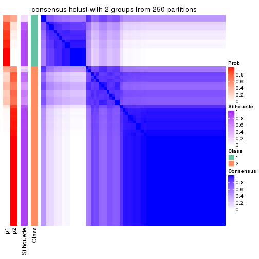
consensus_heatmap(res, k = 3)
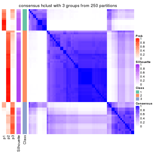
consensus_heatmap(res, k = 4)
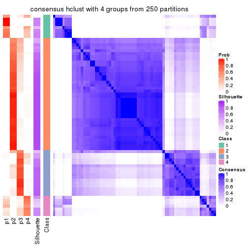
consensus_heatmap(res, k = 5)
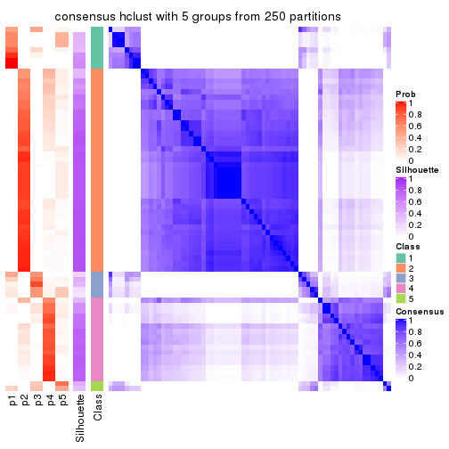
consensus_heatmap(res, k = 6)
Heatmaps for the membership of samples in all partitions to see how consistent they are:
membership_heatmap(res, k = 2)
membership_heatmap(res, k = 3)
membership_heatmap(res, k = 4)
membership_heatmap(res, k = 5)
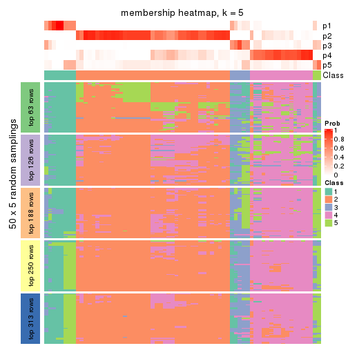
membership_heatmap(res, k = 6)
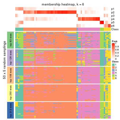
As soon as we have had the classes for columns, we can look for signatures which are significantly different between classes which can be candidate marks for certain classes. Following are the heatmaps for signatures.
Signature heatmaps where rows are scaled:
get_signatures(res, k = 2)
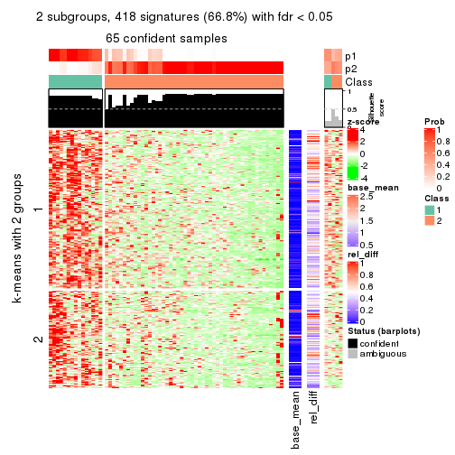
get_signatures(res, k = 3)
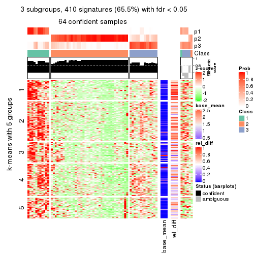
get_signatures(res, k = 4)
get_signatures(res, k = 5)
get_signatures(res, k = 6)
Signature heatmaps where rows are not scaled:
get_signatures(res, k = 2, scale_rows = FALSE)
get_signatures(res, k = 3, scale_rows = FALSE)
get_signatures(res, k = 4, scale_rows = FALSE)
get_signatures(res, k = 5, scale_rows = FALSE)
get_signatures(res, k = 6, scale_rows = FALSE)
Compare the overlap of signatures from different k:
compare_signatures(res)
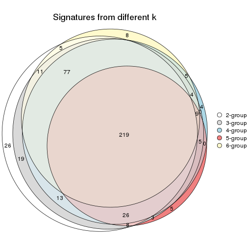
get_signature() returns a data frame invisibly. TO get the list of signatures, the function
call should be assigned to a variable explicitly. In following code, if plot argument is set
to FALSE, no heatmap is plotted while only the differential analysis is performed.
# code only for demonstration
tb = get_signature(res, k = ..., plot = FALSE)
An example of the output of tb is:
#> which_row fdr mean_1 mean_2 scaled_mean_1 scaled_mean_2 km
#> 1 38 0.042760348 8.373488 9.131774 -0.5533452 0.5164555 1
#> 2 40 0.018707592 7.106213 8.469186 -0.6173731 0.5762149 1
#> 3 55 0.019134737 10.221463 11.207825 -0.6159697 0.5749050 1
#> 4 59 0.006059896 5.921854 7.869574 -0.6899429 0.6439467 1
#> 5 60 0.018055526 8.928898 10.211722 -0.6204761 0.5791110 1
#> 6 98 0.009384629 15.714769 14.887706 0.6635654 -0.6193277 2
...
The columns in tb are:
which_row: row indices corresponding to the input matrix.fdr: FDR for the differential test. mean_x: The mean value in group x.scaled_mean_x: The mean value in group x after rows are scaled.km: Row groups if k-means clustering is applied to rows.UMAP plot which shows how samples are separated.
dimension_reduction(res, k = 2, method = "UMAP")

dimension_reduction(res, k = 3, method = "UMAP")
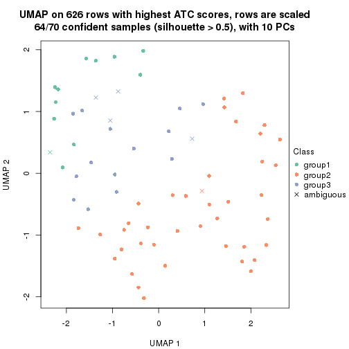
dimension_reduction(res, k = 4, method = "UMAP")
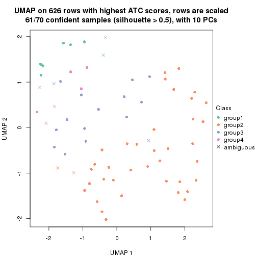
dimension_reduction(res, k = 5, method = "UMAP")
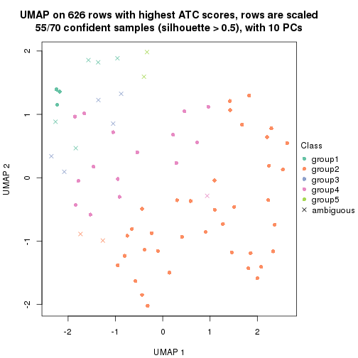
dimension_reduction(res, k = 6, method = "UMAP")
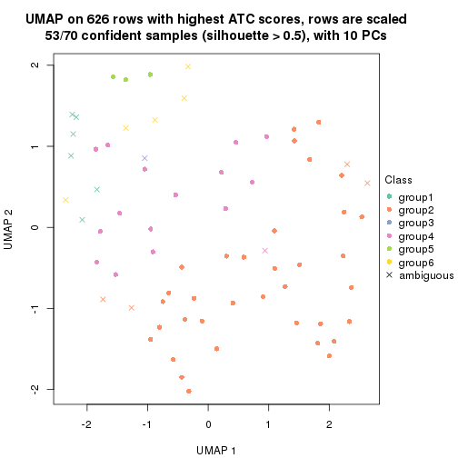
Following heatmap shows how subgroups are split when increasing k:
collect_classes(res)
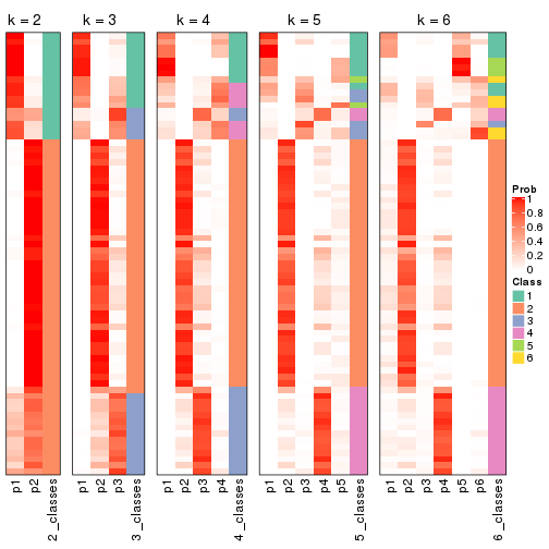
If matrix rows can be associated to genes, consider to use functional_enrichment(res,
...) to perform function enrichment for the signature genes. See this vignette for more detailed explanations.
The object with results only for a single top-value method and a single partition method can be extracted as:
res = res_list["ATC", "kmeans"]
# you can also extract it by
# res = res_list["ATC:kmeans"]
A summary of res and all the functions that can be applied to it:
res
#> A 'ConsensusPartition' object with k = 2, 3, 4, 5, 6.
#> On a matrix with 626 rows and 70 columns.
#> Top rows (63, 126, 188, 250, 313) are extracted by 'ATC' method.
#> Subgroups are detected by 'kmeans' method.
#> Performed in total 1250 partitions by row resampling.
#> Best k for subgroups seems to be 2.
#>
#> Following methods can be applied to this 'ConsensusPartition' object:
#> [1] "cola_report" "collect_classes" "collect_plots"
#> [4] "collect_stats" "colnames" "compare_signatures"
#> [7] "consensus_heatmap" "dimension_reduction" "functional_enrichment"
#> [10] "get_anno_col" "get_anno" "get_classes"
#> [13] "get_consensus" "get_matrix" "get_membership"
#> [16] "get_param" "get_signatures" "get_stats"
#> [19] "is_best_k" "is_stable_k" "membership_heatmap"
#> [22] "ncol" "nrow" "plot_ecdf"
#> [25] "rownames" "select_partition_number" "show"
#> [28] "suggest_best_k" "test_to_known_factors"
collect_plots() function collects all the plots made from res for all k (number of partitions)
into one single page to provide an easy and fast comparison between different k.
collect_plots(res)
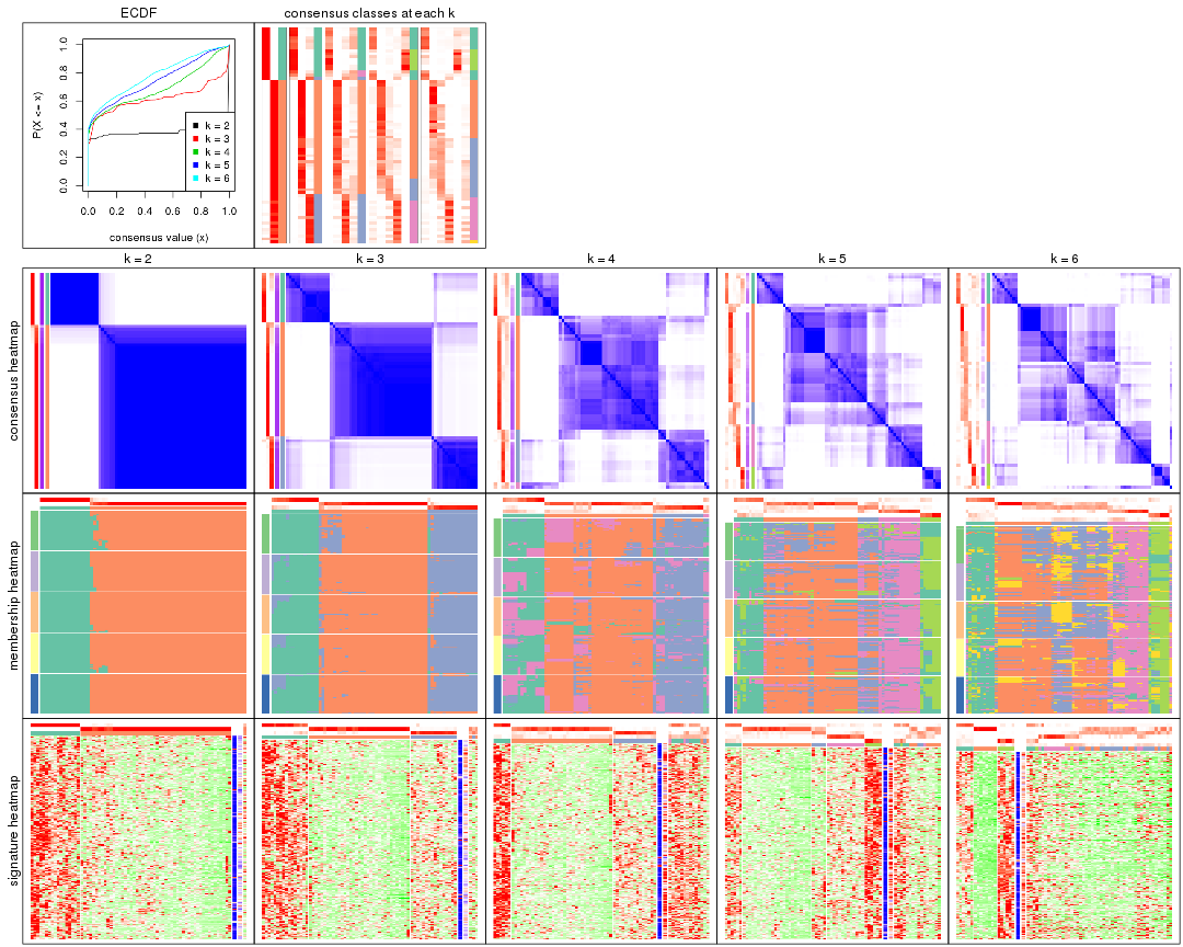
The plots are:
k and the heatmap of
predicted classes for each k.k.k.k.All the plots in panels can be made by individual functions and they are plotted later in this section.
select_partition_number() produces several plots showing different
statistics for choosing “optimized” k. There are following statistics:
k;k, the area increased is defined as \(A_k - A_{k-1}\).The detailed explanations of these statistics can be found in the cola vignette.
Generally speaking, lower PAC score, higher mean silhouette score or higher
concordance corresponds to better partition. Rand index and Jaccard index
measure how similar the current partition is compared to partition with k-1.
If they are too similar, we won't accept k is better than k-1.
select_partition_number(res)
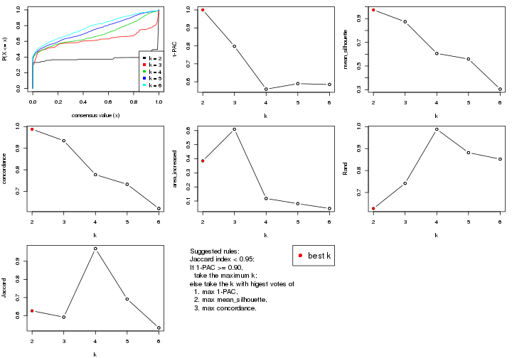
The numeric values for all these statistics can be obtained by get_stats().
get_stats(res)
#> k 1-PAC mean_silhouette concordance area_increased Rand Jaccard
#> 2 2 1.000 0.974 0.988 0.3850 0.627 0.627
#> 3 3 0.798 0.874 0.935 0.6092 0.742 0.592
#> 4 4 0.559 0.606 0.777 0.1183 0.988 0.970
#> 5 5 0.590 0.559 0.733 0.0814 0.882 0.691
#> 6 6 0.585 0.304 0.621 0.0472 0.852 0.533
suggest_best_k() suggests the best \(k\) based on these statistics. The rules are as follows:
suggest_best_k(res)
#> [1] 2
Following shows the table of the partitions (You need to click the show/hide
code output link to see it). The membership matrix (columns with name p*)
is inferred by
clue::cl_consensus()
function with the SE method. Basically the value in the membership matrix
represents the probability to belong to a certain group. The finall class
label for an item is determined with the group with highest probability it
belongs to.
In get_classes() function, the entropy is calculated from the membership
matrix and the silhouette score is calculated from the consensus matrix.
cbind(get_classes(res, k = 2), get_membership(res, k = 2))
#> class entropy silhouette p1 p2
#> SRR837437 2 0.0000 0.984 0.000 1.000
#> SRR837438 2 0.4562 0.897 0.096 0.904
#> SRR837439 2 0.0000 0.984 0.000 1.000
#> SRR837440 2 0.0000 0.984 0.000 1.000
#> SRR837441 2 0.0000 0.984 0.000 1.000
#> SRR837442 2 0.0000 0.984 0.000 1.000
#> SRR837443 2 0.0000 0.984 0.000 1.000
#> SRR837444 2 0.0000 0.984 0.000 1.000
#> SRR837445 2 0.0000 0.984 0.000 1.000
#> SRR837446 2 0.0000 0.984 0.000 1.000
#> SRR837447 1 0.0000 1.000 1.000 0.000
#> SRR837448 1 0.0000 1.000 1.000 0.000
#> SRR837449 1 0.0000 1.000 1.000 0.000
#> SRR837450 1 0.0000 1.000 1.000 0.000
#> SRR837451 2 0.0000 0.984 0.000 1.000
#> SRR837452 2 0.0000 0.984 0.000 1.000
#> SRR837453 2 0.0000 0.984 0.000 1.000
#> SRR837454 2 0.0000 0.984 0.000 1.000
#> SRR837455 1 0.0000 1.000 1.000 0.000
#> SRR837456 1 0.0000 1.000 1.000 0.000
#> SRR837457 2 0.0000 0.984 0.000 1.000
#> SRR837458 1 0.0000 1.000 1.000 0.000
#> SRR837459 2 0.0000 0.984 0.000 1.000
#> SRR837460 2 0.0000 0.984 0.000 1.000
#> SRR837461 2 0.0000 0.984 0.000 1.000
#> SRR837462 2 0.0376 0.981 0.004 0.996
#> SRR837463 2 0.3584 0.926 0.068 0.932
#> SRR837464 2 0.0000 0.984 0.000 1.000
#> SRR837465 2 0.0000 0.984 0.000 1.000
#> SRR837466 1 0.0000 1.000 1.000 0.000
#> SRR837467 2 0.0000 0.984 0.000 1.000
#> SRR837468 2 0.0000 0.984 0.000 1.000
#> SRR837469 1 0.0000 1.000 1.000 0.000
#> SRR837470 1 0.0000 1.000 1.000 0.000
#> SRR837471 2 0.0000 0.984 0.000 1.000
#> SRR837472 2 0.0000 0.984 0.000 1.000
#> SRR837473 2 0.6048 0.835 0.148 0.852
#> SRR837474 2 0.0000 0.984 0.000 1.000
#> SRR837475 2 0.0000 0.984 0.000 1.000
#> SRR837476 2 0.0000 0.984 0.000 1.000
#> SRR837477 2 0.0000 0.984 0.000 1.000
#> SRR837478 2 0.0000 0.984 0.000 1.000
#> SRR837479 2 0.0000 0.984 0.000 1.000
#> SRR837480 2 0.0000 0.984 0.000 1.000
#> SRR837481 2 0.0000 0.984 0.000 1.000
#> SRR837482 2 0.0000 0.984 0.000 1.000
#> SRR837483 1 0.0000 1.000 1.000 0.000
#> SRR837484 2 0.0000 0.984 0.000 1.000
#> SRR837485 2 0.0000 0.984 0.000 1.000
#> SRR837486 2 0.0000 0.984 0.000 1.000
#> SRR837487 2 0.0000 0.984 0.000 1.000
#> SRR837488 2 0.0000 0.984 0.000 1.000
#> SRR837489 2 0.0000 0.984 0.000 1.000
#> SRR837490 2 0.0000 0.984 0.000 1.000
#> SRR837491 2 0.0000 0.984 0.000 1.000
#> SRR837492 2 0.4815 0.888 0.104 0.896
#> SRR837493 2 0.3274 0.933 0.060 0.940
#> SRR837494 2 0.0000 0.984 0.000 1.000
#> SRR837495 2 0.0000 0.984 0.000 1.000
#> SRR837496 1 0.0000 1.000 1.000 0.000
#> SRR837497 1 0.0000 1.000 1.000 0.000
#> SRR837498 1 0.0000 1.000 1.000 0.000
#> SRR837499 1 0.0000 1.000 1.000 0.000
#> SRR837500 1 0.0000 1.000 1.000 0.000
#> SRR837501 2 0.0000 0.984 0.000 1.000
#> SRR837502 2 0.9427 0.465 0.360 0.640
#> SRR837503 1 0.0000 1.000 1.000 0.000
#> SRR837504 2 0.0000 0.984 0.000 1.000
#> SRR837505 2 0.0000 0.984 0.000 1.000
#> SRR837506 2 0.0000 0.984 0.000 1.000
cbind(get_classes(res, k = 3), get_membership(res, k = 3))
#> class entropy silhouette p1 p2 p3
#> SRR837437 2 0.0000 0.943 0.000 1.000 0.000
#> SRR837438 3 0.0892 0.926 0.000 0.020 0.980
#> SRR837439 2 0.4346 0.789 0.000 0.816 0.184
#> SRR837440 2 0.4178 0.806 0.000 0.828 0.172
#> SRR837441 2 0.4002 0.817 0.000 0.840 0.160
#> SRR837442 2 0.0000 0.943 0.000 1.000 0.000
#> SRR837443 2 0.0000 0.943 0.000 1.000 0.000
#> SRR837444 3 0.1529 0.928 0.000 0.040 0.960
#> SRR837445 3 0.1529 0.928 0.000 0.040 0.960
#> SRR837446 2 0.0424 0.941 0.000 0.992 0.008
#> SRR837447 1 0.0424 0.906 0.992 0.000 0.008
#> SRR837448 1 0.0237 0.904 0.996 0.000 0.004
#> SRR837449 1 0.1163 0.903 0.972 0.000 0.028
#> SRR837450 1 0.0237 0.904 0.996 0.000 0.004
#> SRR837451 2 0.0000 0.943 0.000 1.000 0.000
#> SRR837452 2 0.4002 0.818 0.000 0.840 0.160
#> SRR837453 2 0.0000 0.943 0.000 1.000 0.000
#> SRR837454 2 0.0000 0.943 0.000 1.000 0.000
#> SRR837455 1 0.0424 0.906 0.992 0.000 0.008
#> SRR837456 1 0.0424 0.906 0.992 0.000 0.008
#> SRR837457 2 0.0000 0.943 0.000 1.000 0.000
#> SRR837458 1 0.0237 0.904 0.996 0.000 0.004
#> SRR837459 2 0.0000 0.943 0.000 1.000 0.000
#> SRR837460 2 0.0000 0.943 0.000 1.000 0.000
#> SRR837461 2 0.0237 0.942 0.000 0.996 0.004
#> SRR837462 3 0.1163 0.930 0.000 0.028 0.972
#> SRR837463 3 0.0892 0.926 0.000 0.020 0.980
#> SRR837464 3 0.5968 0.416 0.000 0.364 0.636
#> SRR837465 3 0.1163 0.930 0.000 0.028 0.972
#> SRR837466 1 0.0237 0.904 0.996 0.000 0.004
#> SRR837467 2 0.0000 0.943 0.000 1.000 0.000
#> SRR837468 3 0.1289 0.927 0.000 0.032 0.968
#> SRR837469 1 0.0747 0.905 0.984 0.000 0.016
#> SRR837470 1 0.0424 0.906 0.992 0.000 0.008
#> SRR837471 2 0.6291 0.138 0.000 0.532 0.468
#> SRR837472 2 0.4002 0.818 0.000 0.840 0.160
#> SRR837473 3 0.1031 0.929 0.000 0.024 0.976
#> SRR837474 2 0.2625 0.887 0.000 0.916 0.084
#> SRR837475 2 0.0000 0.943 0.000 1.000 0.000
#> SRR837476 2 0.0424 0.940 0.000 0.992 0.008
#> SRR837477 3 0.1411 0.928 0.000 0.036 0.964
#> SRR837478 2 0.0237 0.942 0.000 0.996 0.004
#> SRR837479 2 0.1753 0.919 0.000 0.952 0.048
#> SRR837480 2 0.0747 0.938 0.000 0.984 0.016
#> SRR837481 2 0.0892 0.937 0.000 0.980 0.020
#> SRR837482 3 0.3116 0.845 0.000 0.108 0.892
#> SRR837483 1 0.3686 0.847 0.860 0.000 0.140
#> SRR837484 2 0.0424 0.940 0.000 0.992 0.008
#> SRR837485 2 0.0237 0.941 0.000 0.996 0.004
#> SRR837486 2 0.6062 0.403 0.000 0.616 0.384
#> SRR837487 2 0.0000 0.943 0.000 1.000 0.000
#> SRR837488 2 0.0000 0.943 0.000 1.000 0.000
#> SRR837489 2 0.0000 0.943 0.000 1.000 0.000
#> SRR837490 2 0.0000 0.943 0.000 1.000 0.000
#> SRR837491 3 0.1411 0.930 0.000 0.036 0.964
#> SRR837492 3 0.1031 0.929 0.000 0.024 0.976
#> SRR837493 3 0.0892 0.926 0.000 0.020 0.980
#> SRR837494 2 0.0000 0.943 0.000 1.000 0.000
#> SRR837495 3 0.2261 0.902 0.000 0.068 0.932
#> SRR837496 1 0.4452 0.823 0.808 0.000 0.192
#> SRR837497 1 0.5291 0.739 0.732 0.000 0.268
#> SRR837498 1 0.4399 0.824 0.812 0.000 0.188
#> SRR837499 1 0.6062 0.537 0.616 0.000 0.384
#> SRR837500 3 0.4702 0.617 0.212 0.000 0.788
#> SRR837501 2 0.1860 0.919 0.000 0.948 0.052
#> SRR837502 3 0.1015 0.917 0.008 0.012 0.980
#> SRR837503 1 0.4605 0.812 0.796 0.000 0.204
#> SRR837504 2 0.0000 0.943 0.000 1.000 0.000
#> SRR837505 2 0.0424 0.940 0.000 0.992 0.008
#> SRR837506 2 0.0747 0.935 0.000 0.984 0.016
cbind(get_classes(res, k = 4), get_membership(res, k = 4))
#> class entropy silhouette p1 p2 p3 p4
#> SRR837437 2 0.1302 0.8237 0.000 0.956 0.000 0.044
#> SRR837438 3 0.1716 0.7463 0.000 0.000 0.936 0.064
#> SRR837439 2 0.5102 0.7186 0.000 0.748 0.188 0.064
#> SRR837440 2 0.5073 0.7121 0.000 0.744 0.200 0.056
#> SRR837441 2 0.4804 0.7452 0.000 0.776 0.160 0.064
#> SRR837442 2 0.1209 0.8277 0.000 0.964 0.004 0.032
#> SRR837443 2 0.2586 0.8166 0.000 0.912 0.040 0.048
#> SRR837444 3 0.1510 0.7737 0.000 0.028 0.956 0.016
#> SRR837445 3 0.3333 0.7600 0.000 0.040 0.872 0.088
#> SRR837446 2 0.3245 0.8100 0.000 0.880 0.056 0.064
#> SRR837447 1 0.1004 0.5416 0.972 0.000 0.004 0.024
#> SRR837448 1 0.2281 0.5136 0.904 0.000 0.000 0.096
#> SRR837449 1 0.5252 0.2244 0.644 0.000 0.020 0.336
#> SRR837450 1 0.4250 0.4629 0.724 0.000 0.000 0.276
#> SRR837451 2 0.3172 0.7864 0.000 0.840 0.000 0.160
#> SRR837452 2 0.4055 0.7848 0.000 0.832 0.108 0.060
#> SRR837453 2 0.3172 0.7864 0.000 0.840 0.000 0.160
#> SRR837454 2 0.3074 0.7898 0.000 0.848 0.000 0.152
#> SRR837455 1 0.0188 0.5405 0.996 0.000 0.004 0.000
#> SRR837456 1 0.0188 0.5405 0.996 0.000 0.004 0.000
#> SRR837457 2 0.3172 0.7864 0.000 0.840 0.000 0.160
#> SRR837458 1 0.2081 0.5116 0.916 0.000 0.000 0.084
#> SRR837459 2 0.3172 0.7864 0.000 0.840 0.000 0.160
#> SRR837460 2 0.3172 0.7864 0.000 0.840 0.000 0.160
#> SRR837461 2 0.2675 0.8168 0.000 0.908 0.048 0.044
#> SRR837462 3 0.0592 0.7723 0.000 0.000 0.984 0.016
#> SRR837463 3 0.1302 0.7597 0.000 0.000 0.956 0.044
#> SRR837464 3 0.7004 0.4627 0.000 0.200 0.580 0.220
#> SRR837465 3 0.0657 0.7742 0.000 0.004 0.984 0.012
#> SRR837466 1 0.2281 0.5136 0.904 0.000 0.000 0.096
#> SRR837467 2 0.2313 0.8196 0.000 0.924 0.032 0.044
#> SRR837468 3 0.5995 0.5634 0.000 0.084 0.660 0.256
#> SRR837469 1 0.4122 0.4295 0.760 0.000 0.004 0.236
#> SRR837470 1 0.4304 0.3973 0.716 0.000 0.000 0.284
#> SRR837471 2 0.6953 0.1193 0.000 0.476 0.412 0.112
#> SRR837472 2 0.4547 0.7744 0.000 0.804 0.104 0.092
#> SRR837473 3 0.3356 0.7049 0.000 0.000 0.824 0.176
#> SRR837474 2 0.3764 0.7978 0.000 0.852 0.072 0.076
#> SRR837475 2 0.1767 0.8246 0.000 0.944 0.012 0.044
#> SRR837476 2 0.2996 0.8142 0.000 0.892 0.044 0.064
#> SRR837477 3 0.3876 0.7477 0.000 0.040 0.836 0.124
#> SRR837478 2 0.1302 0.8253 0.000 0.956 0.000 0.044
#> SRR837479 2 0.6592 0.5935 0.000 0.612 0.128 0.260
#> SRR837480 2 0.5723 0.6808 0.000 0.684 0.072 0.244
#> SRR837481 2 0.6084 0.6505 0.000 0.656 0.092 0.252
#> SRR837482 3 0.5989 0.5672 0.000 0.080 0.656 0.264
#> SRR837483 4 0.7264 0.1468 0.392 0.000 0.148 0.460
#> SRR837484 2 0.1716 0.8198 0.000 0.936 0.000 0.064
#> SRR837485 2 0.1389 0.8233 0.000 0.952 0.000 0.048
#> SRR837486 2 0.7849 0.0942 0.000 0.400 0.316 0.284
#> SRR837487 2 0.1118 0.8255 0.000 0.964 0.000 0.036
#> SRR837488 2 0.3172 0.7864 0.000 0.840 0.000 0.160
#> SRR837489 2 0.1724 0.8254 0.000 0.948 0.020 0.032
#> SRR837490 2 0.0804 0.8271 0.000 0.980 0.012 0.008
#> SRR837491 3 0.1798 0.7767 0.000 0.016 0.944 0.040
#> SRR837492 3 0.2868 0.7399 0.000 0.000 0.864 0.136
#> SRR837493 3 0.1637 0.7528 0.000 0.000 0.940 0.060
#> SRR837494 2 0.3172 0.7864 0.000 0.840 0.000 0.160
#> SRR837495 3 0.3873 0.7441 0.000 0.060 0.844 0.096
#> SRR837496 1 0.6953 -0.2343 0.476 0.000 0.112 0.412
#> SRR837497 1 0.7446 -0.4156 0.432 0.000 0.172 0.396
#> SRR837498 1 0.6783 -0.1534 0.512 0.000 0.100 0.388
#> SRR837499 4 0.7867 0.4150 0.292 0.000 0.316 0.392
#> SRR837500 3 0.6607 -0.3019 0.084 0.000 0.516 0.400
#> SRR837501 2 0.7016 0.5335 0.000 0.572 0.176 0.252
#> SRR837502 3 0.3400 0.6309 0.000 0.000 0.820 0.180
#> SRR837503 1 0.7049 -0.2411 0.484 0.000 0.124 0.392
#> SRR837504 2 0.1109 0.8262 0.000 0.968 0.004 0.028
#> SRR837505 2 0.4910 0.7400 0.000 0.704 0.020 0.276
#> SRR837506 2 0.4585 0.6938 0.000 0.668 0.000 0.332
cbind(get_classes(res, k = 5), get_membership(res, k = 5))
#> class entropy silhouette p1 p2 p3 p4 p5
#> SRR837437 2 0.0955 0.6736 0.004 0.968 0.028 0.000 0.000
#> SRR837438 4 0.2130 0.7560 0.080 0.000 0.012 0.908 0.000
#> SRR837439 2 0.6062 0.3902 0.008 0.596 0.148 0.248 0.000
#> SRR837440 2 0.5902 0.4348 0.008 0.628 0.196 0.168 0.000
#> SRR837441 2 0.5740 0.4870 0.008 0.648 0.156 0.188 0.000
#> SRR837442 2 0.1725 0.6703 0.000 0.936 0.044 0.020 0.000
#> SRR837443 2 0.3803 0.6176 0.000 0.804 0.140 0.056 0.000
#> SRR837444 4 0.1788 0.7375 0.008 0.004 0.056 0.932 0.000
#> SRR837445 4 0.4681 0.6936 0.060 0.012 0.184 0.744 0.000
#> SRR837446 2 0.4558 0.5424 0.000 0.728 0.208 0.064 0.000
#> SRR837447 5 0.4793 0.6011 0.232 0.000 0.068 0.000 0.700
#> SRR837448 5 0.0290 0.7512 0.008 0.000 0.000 0.000 0.992
#> SRR837449 1 0.4937 0.5777 0.672 0.000 0.064 0.000 0.264
#> SRR837450 5 0.4292 0.2794 0.272 0.000 0.024 0.000 0.704
#> SRR837451 2 0.4113 0.6166 0.076 0.784 0.140 0.000 0.000
#> SRR837452 2 0.5231 0.5437 0.012 0.704 0.184 0.100 0.000
#> SRR837453 2 0.4113 0.6166 0.076 0.784 0.140 0.000 0.000
#> SRR837454 2 0.4010 0.6200 0.072 0.792 0.136 0.000 0.000
#> SRR837455 5 0.3914 0.7096 0.164 0.000 0.048 0.000 0.788
#> SRR837456 5 0.3914 0.7096 0.164 0.000 0.048 0.000 0.788
#> SRR837457 2 0.4113 0.6166 0.076 0.784 0.140 0.000 0.000
#> SRR837458 5 0.0000 0.7512 0.000 0.000 0.000 0.000 1.000
#> SRR837459 2 0.4113 0.6166 0.076 0.784 0.140 0.000 0.000
#> SRR837460 2 0.4113 0.6166 0.076 0.784 0.140 0.000 0.000
#> SRR837461 2 0.4177 0.5918 0.000 0.772 0.164 0.064 0.000
#> SRR837462 4 0.1549 0.7645 0.040 0.000 0.016 0.944 0.000
#> SRR837463 4 0.2233 0.7579 0.080 0.000 0.016 0.904 0.000
#> SRR837464 4 0.6011 -0.2156 0.004 0.100 0.404 0.492 0.000
#> SRR837465 4 0.1568 0.7640 0.036 0.000 0.020 0.944 0.000
#> SRR837466 5 0.0290 0.7512 0.008 0.000 0.000 0.000 0.992
#> SRR837467 2 0.3692 0.6157 0.000 0.812 0.136 0.052 0.000
#> SRR837468 3 0.4684 0.1132 0.004 0.008 0.536 0.452 0.000
#> SRR837469 1 0.5295 0.2784 0.540 0.000 0.052 0.000 0.408
#> SRR837470 1 0.5320 0.2459 0.488 0.000 0.040 0.004 0.468
#> SRR837471 2 0.7776 -0.1235 0.064 0.356 0.236 0.344 0.000
#> SRR837472 2 0.6546 0.3974 0.052 0.592 0.244 0.112 0.000
#> SRR837473 4 0.5271 0.6985 0.168 0.000 0.152 0.680 0.000
#> SRR837474 2 0.5887 0.4732 0.028 0.644 0.232 0.096 0.000
#> SRR837475 2 0.4117 0.6094 0.020 0.804 0.128 0.048 0.000
#> SRR837476 2 0.4622 0.6027 0.012 0.760 0.152 0.076 0.000
#> SRR837477 4 0.5782 0.5820 0.072 0.016 0.320 0.592 0.000
#> SRR837478 2 0.2006 0.6693 0.012 0.916 0.072 0.000 0.000
#> SRR837479 3 0.5172 0.5880 0.008 0.380 0.580 0.032 0.000
#> SRR837480 3 0.4582 0.5376 0.000 0.416 0.572 0.012 0.000
#> SRR837481 3 0.4856 0.5756 0.004 0.392 0.584 0.020 0.000
#> SRR837482 3 0.5161 0.1969 0.012 0.024 0.568 0.396 0.000
#> SRR837483 1 0.5902 0.3538 0.528 0.000 0.028 0.048 0.396
#> SRR837484 2 0.1943 0.6628 0.020 0.924 0.056 0.000 0.000
#> SRR837485 2 0.1364 0.6702 0.012 0.952 0.036 0.000 0.000
#> SRR837486 3 0.5386 0.5984 0.004 0.192 0.676 0.128 0.000
#> SRR837487 2 0.1251 0.6727 0.008 0.956 0.036 0.000 0.000
#> SRR837488 2 0.4113 0.6166 0.076 0.784 0.140 0.000 0.000
#> SRR837489 2 0.3401 0.6526 0.008 0.852 0.072 0.068 0.000
#> SRR837490 2 0.1822 0.6732 0.004 0.936 0.024 0.036 0.000
#> SRR837491 4 0.2409 0.7579 0.032 0.000 0.068 0.900 0.000
#> SRR837492 4 0.5538 0.6912 0.144 0.000 0.212 0.644 0.000
#> SRR837493 4 0.2110 0.7651 0.072 0.000 0.016 0.912 0.000
#> SRR837494 2 0.4113 0.6166 0.076 0.784 0.140 0.000 0.000
#> SRR837495 4 0.5484 0.6271 0.060 0.032 0.232 0.676 0.000
#> SRR837496 1 0.4393 0.6975 0.752 0.000 0.004 0.052 0.192
#> SRR837497 1 0.4758 0.6966 0.748 0.000 0.016 0.068 0.168
#> SRR837498 1 0.4971 0.6718 0.716 0.000 0.032 0.036 0.216
#> SRR837499 1 0.4922 0.6373 0.732 0.000 0.008 0.156 0.104
#> SRR837500 1 0.4353 0.3958 0.660 0.000 0.008 0.328 0.004
#> SRR837501 3 0.5669 0.6247 0.008 0.328 0.588 0.076 0.000
#> SRR837502 4 0.3519 0.6661 0.216 0.000 0.008 0.776 0.000
#> SRR837503 1 0.4359 0.6977 0.752 0.000 0.004 0.048 0.196
#> SRR837504 2 0.2824 0.6436 0.000 0.864 0.116 0.020 0.000
#> SRR837505 2 0.5109 -0.1392 0.036 0.504 0.460 0.000 0.000
#> SRR837506 2 0.5803 0.0819 0.092 0.488 0.420 0.000 0.000
cbind(get_classes(res, k = 6), get_membership(res, k = 6))
#> class entropy silhouette p1 p2 p3 p4 p5 p6
#> SRR837437 2 0.4154 0.45035 0.004 0.652 0.324 0.000 0.000 0.020
#> SRR837438 4 0.1471 0.46041 0.064 0.000 0.000 0.932 0.000 0.004
#> SRR837439 3 0.6940 0.23467 0.008 0.260 0.420 0.268 0.000 0.044
#> SRR837440 3 0.6585 0.21988 0.012 0.316 0.484 0.148 0.000 0.040
#> SRR837441 3 0.6768 0.18411 0.008 0.332 0.436 0.180 0.000 0.044
#> SRR837442 2 0.4719 0.30053 0.004 0.560 0.400 0.004 0.000 0.032
#> SRR837443 3 0.5014 -0.11802 0.008 0.468 0.484 0.012 0.000 0.028
#> SRR837444 4 0.2030 0.41650 0.000 0.000 0.064 0.908 0.000 0.028
#> SRR837445 4 0.5206 -0.48603 0.000 0.000 0.116 0.572 0.000 0.312
#> SRR837446 3 0.4627 0.00906 0.004 0.400 0.568 0.012 0.000 0.016
#> SRR837447 5 0.5480 0.60819 0.172 0.000 0.020 0.000 0.628 0.180
#> SRR837448 5 0.0291 0.73688 0.004 0.000 0.000 0.000 0.992 0.004
#> SRR837449 1 0.5317 0.60696 0.680 0.000 0.016 0.016 0.140 0.148
#> SRR837450 5 0.4697 0.09743 0.324 0.000 0.000 0.000 0.612 0.064
#> SRR837451 2 0.0000 0.59035 0.000 1.000 0.000 0.000 0.000 0.000
#> SRR837452 3 0.5669 0.02453 0.004 0.408 0.492 0.024 0.000 0.072
#> SRR837453 2 0.0000 0.59035 0.000 1.000 0.000 0.000 0.000 0.000
#> SRR837454 2 0.0547 0.58592 0.000 0.980 0.020 0.000 0.000 0.000
#> SRR837455 5 0.4661 0.69520 0.108 0.000 0.020 0.000 0.724 0.148
#> SRR837456 5 0.4661 0.69520 0.108 0.000 0.020 0.000 0.724 0.148
#> SRR837457 2 0.0000 0.59035 0.000 1.000 0.000 0.000 0.000 0.000
#> SRR837458 5 0.0146 0.73753 0.004 0.000 0.000 0.000 0.996 0.000
#> SRR837459 2 0.0000 0.59035 0.000 1.000 0.000 0.000 0.000 0.000
#> SRR837460 2 0.0000 0.59035 0.000 1.000 0.000 0.000 0.000 0.000
#> SRR837461 3 0.5349 -0.05223 0.008 0.444 0.488 0.024 0.000 0.036
#> SRR837462 4 0.0725 0.46870 0.012 0.000 0.012 0.976 0.000 0.000
#> SRR837463 4 0.0865 0.46899 0.036 0.000 0.000 0.964 0.000 0.000
#> SRR837464 4 0.6745 0.02266 0.040 0.020 0.348 0.452 0.000 0.140
#> SRR837465 4 0.0922 0.46237 0.004 0.000 0.024 0.968 0.000 0.004
#> SRR837466 5 0.0291 0.73688 0.004 0.000 0.000 0.000 0.992 0.004
#> SRR837467 2 0.5036 0.10475 0.004 0.484 0.464 0.012 0.000 0.036
#> SRR837468 4 0.6603 0.00354 0.032 0.000 0.312 0.412 0.000 0.244
#> SRR837469 1 0.6078 0.48873 0.568 0.000 0.032 0.004 0.232 0.164
#> SRR837470 1 0.5712 0.44405 0.552 0.000 0.020 0.000 0.308 0.120
#> SRR837471 3 0.6987 -0.11314 0.004 0.100 0.416 0.132 0.000 0.348
#> SRR837472 3 0.6367 0.19770 0.004 0.292 0.444 0.012 0.000 0.248
#> SRR837473 4 0.6249 -0.53578 0.084 0.000 0.072 0.472 0.000 0.372
#> SRR837474 3 0.6034 0.14797 0.000 0.332 0.476 0.012 0.000 0.180
#> SRR837475 3 0.5710 -0.02073 0.000 0.412 0.444 0.004 0.000 0.140
#> SRR837476 3 0.5582 0.03726 0.000 0.388 0.492 0.008 0.000 0.112
#> SRR837477 6 0.6231 0.00000 0.012 0.000 0.180 0.400 0.004 0.404
#> SRR837478 2 0.4791 0.41654 0.008 0.612 0.328 0.000 0.000 0.052
#> SRR837479 3 0.6452 0.29873 0.040 0.128 0.568 0.020 0.004 0.240
#> SRR837480 3 0.5798 0.32665 0.028 0.156 0.608 0.004 0.000 0.204
#> SRR837481 3 0.5757 0.33226 0.028 0.144 0.624 0.008 0.000 0.196
#> SRR837482 3 0.6680 -0.24578 0.040 0.000 0.424 0.288 0.000 0.248
#> SRR837483 1 0.6144 0.38628 0.528 0.000 0.024 0.020 0.328 0.100
#> SRR837484 2 0.4268 0.49182 0.008 0.692 0.264 0.000 0.000 0.036
#> SRR837485 2 0.4350 0.48283 0.008 0.676 0.280 0.000 0.000 0.036
#> SRR837486 3 0.6264 0.12527 0.036 0.040 0.588 0.072 0.004 0.260
#> SRR837487 2 0.4245 0.44184 0.004 0.644 0.328 0.000 0.000 0.024
#> SRR837488 2 0.0000 0.59035 0.000 1.000 0.000 0.000 0.000 0.000
#> SRR837489 2 0.5300 0.05750 0.000 0.464 0.452 0.008 0.000 0.076
#> SRR837490 2 0.4334 0.29554 0.000 0.568 0.408 0.000 0.000 0.024
#> SRR837491 4 0.3076 0.32299 0.004 0.000 0.044 0.840 0.000 0.112
#> SRR837492 4 0.6302 -0.67469 0.052 0.000 0.100 0.468 0.004 0.376
#> SRR837493 4 0.1890 0.45561 0.060 0.000 0.000 0.916 0.000 0.024
#> SRR837494 2 0.0000 0.59035 0.000 1.000 0.000 0.000 0.000 0.000
#> SRR837495 4 0.5890 -0.62951 0.000 0.000 0.212 0.448 0.000 0.340
#> SRR837496 1 0.3201 0.72207 0.852 0.000 0.008 0.024 0.092 0.024
#> SRR837497 1 0.4748 0.71815 0.768 0.000 0.036 0.044 0.084 0.068
#> SRR837498 1 0.4939 0.70671 0.748 0.000 0.028 0.040 0.088 0.096
#> SRR837499 1 0.4107 0.68073 0.780 0.000 0.000 0.128 0.060 0.032
#> SRR837500 1 0.4517 0.45163 0.648 0.000 0.000 0.292 0.000 0.060
#> SRR837501 3 0.6946 0.28859 0.056 0.120 0.528 0.048 0.000 0.248
#> SRR837502 4 0.3922 0.29792 0.124 0.000 0.004 0.776 0.000 0.096
#> SRR837503 1 0.3247 0.72158 0.848 0.000 0.008 0.028 0.096 0.020
#> SRR837504 2 0.4755 0.15694 0.008 0.512 0.452 0.004 0.000 0.024
#> SRR837505 3 0.6228 0.15634 0.028 0.360 0.456 0.000 0.000 0.156
#> SRR837506 2 0.5961 0.07327 0.040 0.580 0.228 0.000 0.000 0.152
Heatmaps for the consensus matrix. It visualizes the probability of two samples to be in a same group.
consensus_heatmap(res, k = 2)
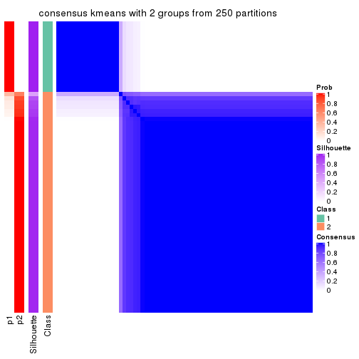
consensus_heatmap(res, k = 3)
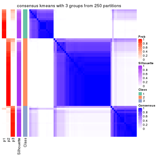
consensus_heatmap(res, k = 4)
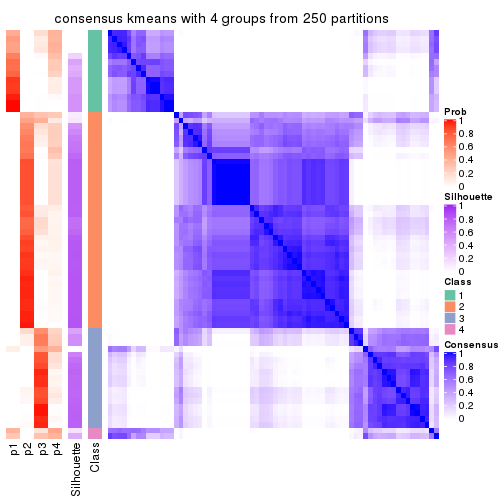
consensus_heatmap(res, k = 5)
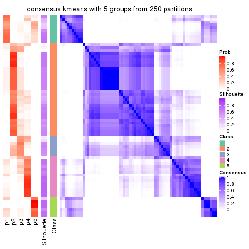
consensus_heatmap(res, k = 6)
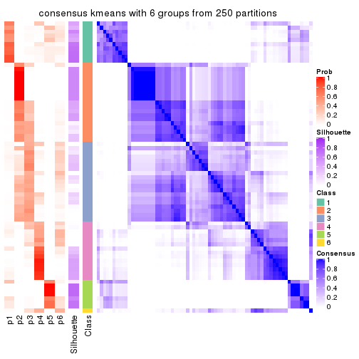
Heatmaps for the membership of samples in all partitions to see how consistent they are:
membership_heatmap(res, k = 2)
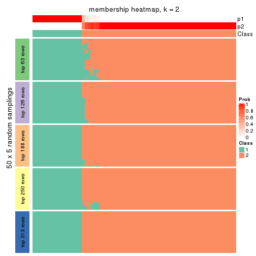
membership_heatmap(res, k = 3)
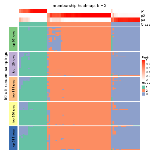
membership_heatmap(res, k = 4)
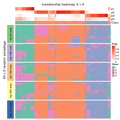
membership_heatmap(res, k = 5)
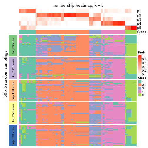
membership_heatmap(res, k = 6)
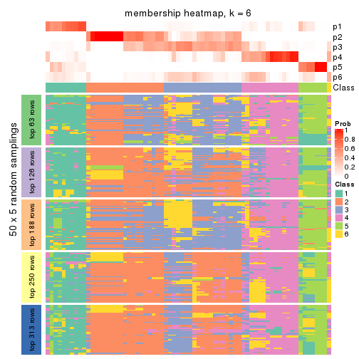
As soon as we have had the classes for columns, we can look for signatures which are significantly different between classes which can be candidate marks for certain classes. Following are the heatmaps for signatures.
Signature heatmaps where rows are scaled:
get_signatures(res, k = 2)
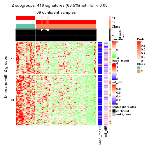
get_signatures(res, k = 3)
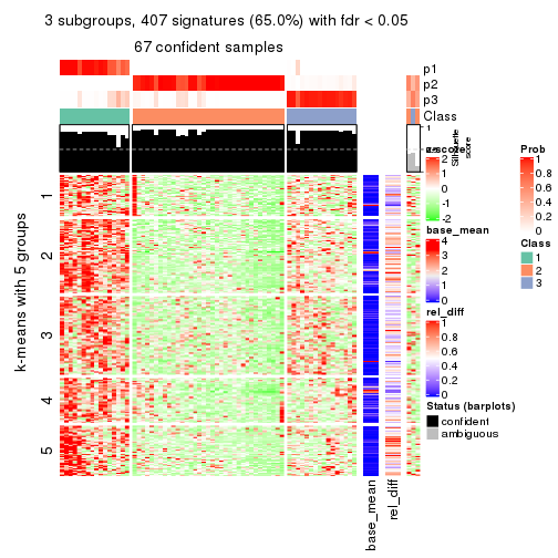
get_signatures(res, k = 4)
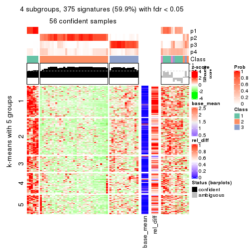
get_signatures(res, k = 5)
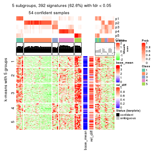
get_signatures(res, k = 6)
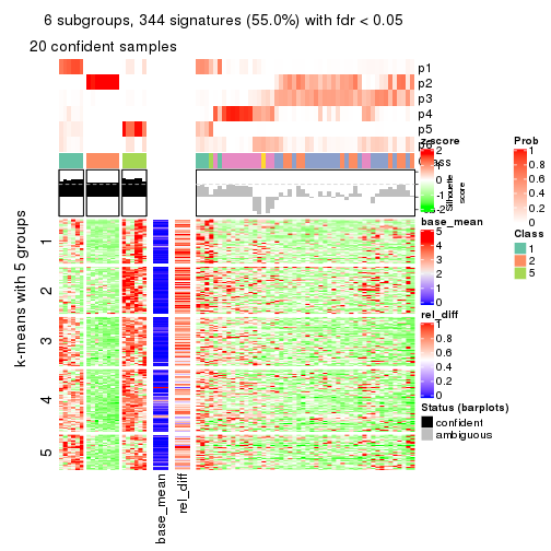
Signature heatmaps where rows are not scaled:
get_signatures(res, k = 2, scale_rows = FALSE)
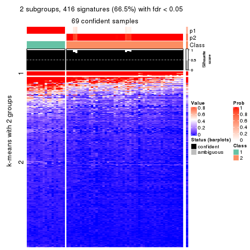
get_signatures(res, k = 3, scale_rows = FALSE)
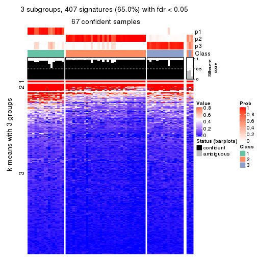
get_signatures(res, k = 4, scale_rows = FALSE)
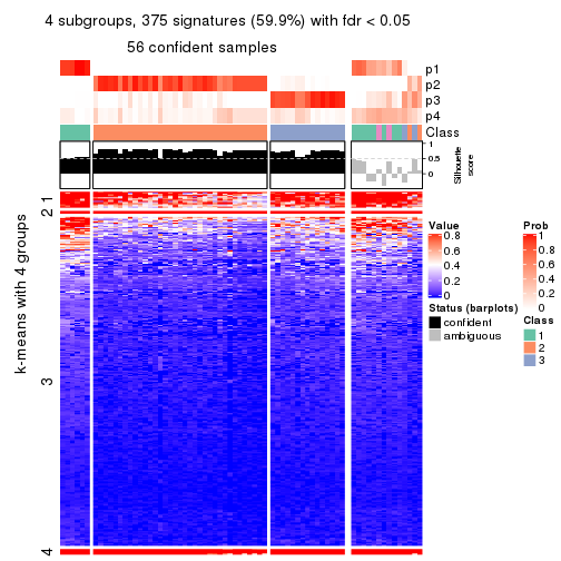
get_signatures(res, k = 5, scale_rows = FALSE)
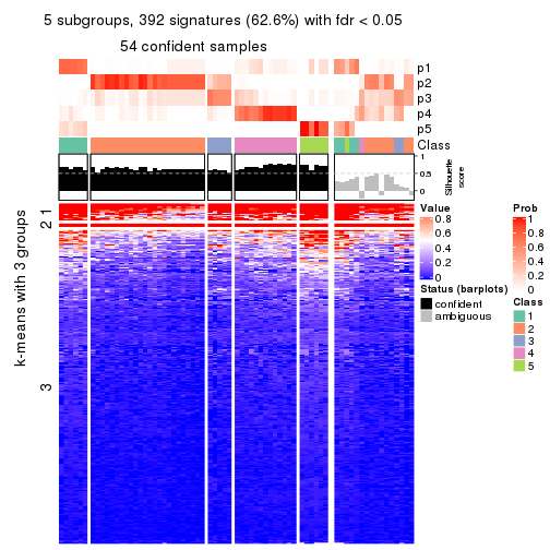
get_signatures(res, k = 6, scale_rows = FALSE)
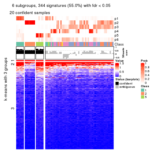
Compare the overlap of signatures from different k:
compare_signatures(res)
get_signature() returns a data frame invisibly. TO get the list of signatures, the function
call should be assigned to a variable explicitly. In following code, if plot argument is set
to FALSE, no heatmap is plotted while only the differential analysis is performed.
# code only for demonstration
tb = get_signature(res, k = ..., plot = FALSE)
An example of the output of tb is:
#> which_row fdr mean_1 mean_2 scaled_mean_1 scaled_mean_2 km
#> 1 38 0.042760348 8.373488 9.131774 -0.5533452 0.5164555 1
#> 2 40 0.018707592 7.106213 8.469186 -0.6173731 0.5762149 1
#> 3 55 0.019134737 10.221463 11.207825 -0.6159697 0.5749050 1
#> 4 59 0.006059896 5.921854 7.869574 -0.6899429 0.6439467 1
#> 5 60 0.018055526 8.928898 10.211722 -0.6204761 0.5791110 1
#> 6 98 0.009384629 15.714769 14.887706 0.6635654 -0.6193277 2
...
The columns in tb are:
which_row: row indices corresponding to the input matrix.fdr: FDR for the differential test. mean_x: The mean value in group x.scaled_mean_x: The mean value in group x after rows are scaled.km: Row groups if k-means clustering is applied to rows.UMAP plot which shows how samples are separated.
dimension_reduction(res, k = 2, method = "UMAP")
dimension_reduction(res, k = 3, method = "UMAP")
dimension_reduction(res, k = 4, method = "UMAP")

dimension_reduction(res, k = 5, method = "UMAP")
dimension_reduction(res, k = 6, method = "UMAP")
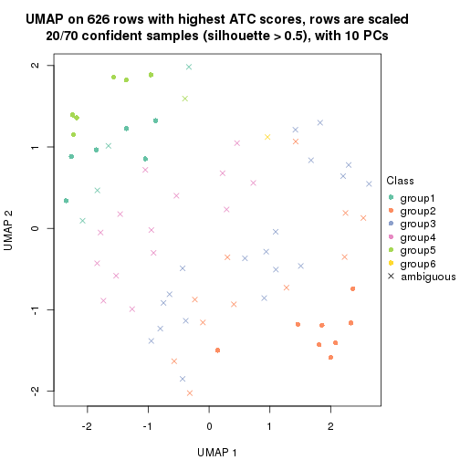
Following heatmap shows how subgroups are split when increasing k:
collect_classes(res)
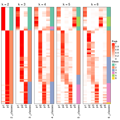
If matrix rows can be associated to genes, consider to use functional_enrichment(res,
...) to perform function enrichment for the signature genes. See this vignette for more detailed explanations.
The object with results only for a single top-value method and a single partition method can be extracted as:
res = res_list["ATC", "skmeans"]
# you can also extract it by
# res = res_list["ATC:skmeans"]
A summary of res and all the functions that can be applied to it:
res
#> A 'ConsensusPartition' object with k = 2, 3, 4, 5, 6.
#> On a matrix with 626 rows and 70 columns.
#> Top rows (63, 126, 188, 250, 313) are extracted by 'ATC' method.
#> Subgroups are detected by 'skmeans' method.
#> Performed in total 1250 partitions by row resampling.
#> Best k for subgroups seems to be 2.
#>
#> Following methods can be applied to this 'ConsensusPartition' object:
#> [1] "cola_report" "collect_classes" "collect_plots"
#> [4] "collect_stats" "colnames" "compare_signatures"
#> [7] "consensus_heatmap" "dimension_reduction" "functional_enrichment"
#> [10] "get_anno_col" "get_anno" "get_classes"
#> [13] "get_consensus" "get_matrix" "get_membership"
#> [16] "get_param" "get_signatures" "get_stats"
#> [19] "is_best_k" "is_stable_k" "membership_heatmap"
#> [22] "ncol" "nrow" "plot_ecdf"
#> [25] "rownames" "select_partition_number" "show"
#> [28] "suggest_best_k" "test_to_known_factors"
collect_plots() function collects all the plots made from res for all k (number of partitions)
into one single page to provide an easy and fast comparison between different k.
collect_plots(res)
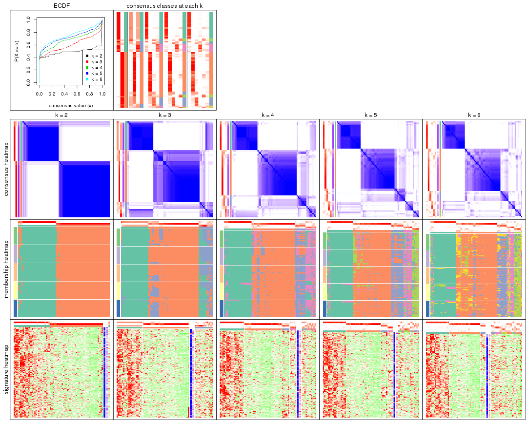
The plots are:
k and the heatmap of
predicted classes for each k.k.k.k.All the plots in panels can be made by individual functions and they are plotted later in this section.
select_partition_number() produces several plots showing different
statistics for choosing “optimized” k. There are following statistics:
k;k, the area increased is defined as \(A_k - A_{k-1}\).The detailed explanations of these statistics can be found in the cola vignette.
Generally speaking, lower PAC score, higher mean silhouette score or higher
concordance corresponds to better partition. Rand index and Jaccard index
measure how similar the current partition is compared to partition with k-1.
If they are too similar, we won't accept k is better than k-1.
select_partition_number(res)

The numeric values for all these statistics can be obtained by get_stats().
get_stats(res)
#> k 1-PAC mean_silhouette concordance area_increased Rand Jaccard
#> 2 2 0.969 0.954 0.980 0.4887 0.508 0.508
#> 3 3 0.702 0.740 0.868 0.2401 0.873 0.755
#> 4 4 0.693 0.706 0.855 0.1252 0.897 0.753
#> 5 5 0.697 0.711 0.856 0.0647 0.927 0.783
#> 6 6 0.685 0.592 0.801 0.0425 0.968 0.892
suggest_best_k() suggests the best \(k\) based on these statistics. The rules are as follows:
suggest_best_k(res)
#> [1] 2
Following shows the table of the partitions (You need to click the show/hide
code output link to see it). The membership matrix (columns with name p*)
is inferred by
clue::cl_consensus()
function with the SE method. Basically the value in the membership matrix
represents the probability to belong to a certain group. The finall class
label for an item is determined with the group with highest probability it
belongs to.
In get_classes() function, the entropy is calculated from the membership
matrix and the silhouette score is calculated from the consensus matrix.
cbind(get_classes(res, k = 2), get_membership(res, k = 2))
#> class entropy silhouette p1 p2
#> SRR837437 2 0.0000 0.991 0.000 1.000
#> SRR837438 1 0.0000 0.961 1.000 0.000
#> SRR837439 2 0.0000 0.991 0.000 1.000
#> SRR837440 2 0.0000 0.991 0.000 1.000
#> SRR837441 2 0.0000 0.991 0.000 1.000
#> SRR837442 2 0.0000 0.991 0.000 1.000
#> SRR837443 2 0.0000 0.991 0.000 1.000
#> SRR837444 1 0.9427 0.460 0.640 0.360
#> SRR837445 2 0.4431 0.896 0.092 0.908
#> SRR837446 2 0.0000 0.991 0.000 1.000
#> SRR837447 1 0.0000 0.961 1.000 0.000
#> SRR837448 1 0.0000 0.961 1.000 0.000
#> SRR837449 1 0.0000 0.961 1.000 0.000
#> SRR837450 1 0.0000 0.961 1.000 0.000
#> SRR837451 2 0.0000 0.991 0.000 1.000
#> SRR837452 2 0.0000 0.991 0.000 1.000
#> SRR837453 2 0.0000 0.991 0.000 1.000
#> SRR837454 2 0.0000 0.991 0.000 1.000
#> SRR837455 1 0.0000 0.961 1.000 0.000
#> SRR837456 1 0.0000 0.961 1.000 0.000
#> SRR837457 2 0.0000 0.991 0.000 1.000
#> SRR837458 1 0.0000 0.961 1.000 0.000
#> SRR837459 2 0.0000 0.991 0.000 1.000
#> SRR837460 2 0.0000 0.991 0.000 1.000
#> SRR837461 2 0.0000 0.991 0.000 1.000
#> SRR837462 1 0.0000 0.961 1.000 0.000
#> SRR837463 1 0.0000 0.961 1.000 0.000
#> SRR837464 2 0.0000 0.991 0.000 1.000
#> SRR837465 1 0.0376 0.958 0.996 0.004
#> SRR837466 1 0.0000 0.961 1.000 0.000
#> SRR837467 2 0.0000 0.991 0.000 1.000
#> SRR837468 1 0.7950 0.699 0.760 0.240
#> SRR837469 1 0.0000 0.961 1.000 0.000
#> SRR837470 1 0.0000 0.961 1.000 0.000
#> SRR837471 2 0.0000 0.991 0.000 1.000
#> SRR837472 2 0.0000 0.991 0.000 1.000
#> SRR837473 1 0.0000 0.961 1.000 0.000
#> SRR837474 2 0.0000 0.991 0.000 1.000
#> SRR837475 2 0.0000 0.991 0.000 1.000
#> SRR837476 2 0.0000 0.991 0.000 1.000
#> SRR837477 1 0.9129 0.540 0.672 0.328
#> SRR837478 2 0.0000 0.991 0.000 1.000
#> SRR837479 2 0.0000 0.991 0.000 1.000
#> SRR837480 2 0.0000 0.991 0.000 1.000
#> SRR837481 2 0.0000 0.991 0.000 1.000
#> SRR837482 2 0.4431 0.897 0.092 0.908
#> SRR837483 1 0.0000 0.961 1.000 0.000
#> SRR837484 2 0.0000 0.991 0.000 1.000
#> SRR837485 2 0.0000 0.991 0.000 1.000
#> SRR837486 2 0.0672 0.984 0.008 0.992
#> SRR837487 2 0.0000 0.991 0.000 1.000
#> SRR837488 2 0.0000 0.991 0.000 1.000
#> SRR837489 2 0.0000 0.991 0.000 1.000
#> SRR837490 2 0.0000 0.991 0.000 1.000
#> SRR837491 1 0.5946 0.823 0.856 0.144
#> SRR837492 1 0.0000 0.961 1.000 0.000
#> SRR837493 1 0.0000 0.961 1.000 0.000
#> SRR837494 2 0.0000 0.991 0.000 1.000
#> SRR837495 2 0.6343 0.804 0.160 0.840
#> SRR837496 1 0.0000 0.961 1.000 0.000
#> SRR837497 1 0.0000 0.961 1.000 0.000
#> SRR837498 1 0.0000 0.961 1.000 0.000
#> SRR837499 1 0.0000 0.961 1.000 0.000
#> SRR837500 1 0.0000 0.961 1.000 0.000
#> SRR837501 2 0.0000 0.991 0.000 1.000
#> SRR837502 1 0.0000 0.961 1.000 0.000
#> SRR837503 1 0.0000 0.961 1.000 0.000
#> SRR837504 2 0.0000 0.991 0.000 1.000
#> SRR837505 2 0.0000 0.991 0.000 1.000
#> SRR837506 2 0.0000 0.991 0.000 1.000
cbind(get_classes(res, k = 3), get_membership(res, k = 3))
#> class entropy silhouette p1 p2 p3
#> SRR837437 2 0.0000 0.8979 0.000 1.000 0.000
#> SRR837438 3 0.6168 -0.7346 0.412 0.000 0.588
#> SRR837439 2 0.3816 0.7846 0.000 0.852 0.148
#> SRR837440 2 0.3695 0.8162 0.012 0.880 0.108
#> SRR837441 2 0.3619 0.7972 0.000 0.864 0.136
#> SRR837442 2 0.0000 0.8979 0.000 1.000 0.000
#> SRR837443 2 0.0747 0.8914 0.000 0.984 0.016
#> SRR837444 3 0.7228 0.5140 0.104 0.188 0.708
#> SRR837445 3 0.9648 0.1728 0.208 0.384 0.408
#> SRR837446 2 0.1643 0.8794 0.044 0.956 0.000
#> SRR837447 1 0.6274 0.9350 0.544 0.000 0.456
#> SRR837448 1 0.6260 0.9360 0.552 0.000 0.448
#> SRR837449 1 0.6274 0.9350 0.544 0.000 0.456
#> SRR837450 1 0.6260 0.9360 0.552 0.000 0.448
#> SRR837451 2 0.0000 0.8979 0.000 1.000 0.000
#> SRR837452 2 0.0000 0.8979 0.000 1.000 0.000
#> SRR837453 2 0.0000 0.8979 0.000 1.000 0.000
#> SRR837454 2 0.0000 0.8979 0.000 1.000 0.000
#> SRR837455 1 0.6274 0.9350 0.544 0.000 0.456
#> SRR837456 1 0.6274 0.9350 0.544 0.000 0.456
#> SRR837457 2 0.0000 0.8979 0.000 1.000 0.000
#> SRR837458 1 0.6260 0.9360 0.552 0.000 0.448
#> SRR837459 2 0.0000 0.8979 0.000 1.000 0.000
#> SRR837460 2 0.0000 0.8979 0.000 1.000 0.000
#> SRR837461 2 0.1267 0.8863 0.004 0.972 0.024
#> SRR837462 3 0.1031 0.3490 0.024 0.000 0.976
#> SRR837463 3 0.1860 0.3039 0.052 0.000 0.948
#> SRR837464 3 0.9322 0.3223 0.192 0.304 0.504
#> SRR837465 3 0.0237 0.3812 0.000 0.004 0.996
#> SRR837466 1 0.6260 0.9360 0.552 0.000 0.448
#> SRR837467 2 0.0000 0.8979 0.000 1.000 0.000
#> SRR837468 3 0.7104 0.4928 0.360 0.032 0.608
#> SRR837469 1 0.6274 0.9350 0.544 0.000 0.456
#> SRR837470 1 0.6260 0.9360 0.552 0.000 0.448
#> SRR837471 2 0.1860 0.8686 0.052 0.948 0.000
#> SRR837472 2 0.1031 0.8897 0.024 0.976 0.000
#> SRR837473 1 0.6126 0.8785 0.600 0.000 0.400
#> SRR837474 2 0.0424 0.8950 0.008 0.992 0.000
#> SRR837475 2 0.0237 0.8966 0.004 0.996 0.000
#> SRR837476 2 0.0000 0.8979 0.000 1.000 0.000
#> SRR837477 1 0.4779 -0.1700 0.840 0.124 0.036
#> SRR837478 2 0.2711 0.8507 0.088 0.912 0.000
#> SRR837479 2 0.6451 0.5394 0.384 0.608 0.008
#> SRR837480 2 0.6026 0.5627 0.376 0.624 0.000
#> SRR837481 2 0.6026 0.5626 0.376 0.624 0.000
#> SRR837482 3 0.9140 0.4232 0.404 0.144 0.452
#> SRR837483 1 0.6260 0.9360 0.552 0.000 0.448
#> SRR837484 2 0.0237 0.8970 0.004 0.996 0.000
#> SRR837485 2 0.0592 0.8944 0.012 0.988 0.000
#> SRR837486 2 0.7236 0.4870 0.392 0.576 0.032
#> SRR837487 2 0.0000 0.8979 0.000 1.000 0.000
#> SRR837488 2 0.0000 0.8979 0.000 1.000 0.000
#> SRR837489 2 0.0000 0.8979 0.000 1.000 0.000
#> SRR837490 2 0.0000 0.8979 0.000 1.000 0.000
#> SRR837491 3 0.7372 0.1676 0.220 0.092 0.688
#> SRR837492 1 0.5988 0.8171 0.632 0.000 0.368
#> SRR837493 3 0.4235 -0.0477 0.176 0.000 0.824
#> SRR837494 2 0.0000 0.8979 0.000 1.000 0.000
#> SRR837495 2 0.6556 0.5801 0.276 0.692 0.032
#> SRR837496 1 0.6260 0.9360 0.552 0.000 0.448
#> SRR837497 1 0.6260 0.9360 0.552 0.000 0.448
#> SRR837498 1 0.6274 0.9350 0.544 0.000 0.456
#> SRR837499 1 0.6274 0.9350 0.544 0.000 0.456
#> SRR837500 1 0.6274 0.9350 0.544 0.000 0.456
#> SRR837501 2 0.8588 0.4345 0.344 0.544 0.112
#> SRR837502 1 0.6295 0.9091 0.528 0.000 0.472
#> SRR837503 1 0.6260 0.9360 0.552 0.000 0.448
#> SRR837504 2 0.0000 0.8979 0.000 1.000 0.000
#> SRR837505 2 0.5058 0.7087 0.244 0.756 0.000
#> SRR837506 2 0.5138 0.6999 0.252 0.748 0.000
cbind(get_classes(res, k = 4), get_membership(res, k = 4))
#> class entropy silhouette p1 p2 p3 p4
#> SRR837437 2 0.0000 0.8616 0.000 1.000 0.000 0.000
#> SRR837438 1 0.4655 0.4119 0.684 0.000 0.004 0.312
#> SRR837439 2 0.4826 0.5859 0.000 0.716 0.020 0.264
#> SRR837440 2 0.3697 0.7637 0.000 0.852 0.048 0.100
#> SRR837441 2 0.4175 0.6827 0.000 0.784 0.016 0.200
#> SRR837442 2 0.0188 0.8610 0.000 0.996 0.004 0.000
#> SRR837443 2 0.0657 0.8571 0.000 0.984 0.004 0.012
#> SRR837444 4 0.3852 0.5141 0.036 0.048 0.048 0.868
#> SRR837445 4 0.7319 0.1605 0.004 0.156 0.316 0.524
#> SRR837446 2 0.2334 0.8003 0.000 0.908 0.088 0.004
#> SRR837447 1 0.0817 0.9214 0.976 0.000 0.000 0.024
#> SRR837448 1 0.0469 0.9195 0.988 0.000 0.000 0.012
#> SRR837449 1 0.0817 0.9214 0.976 0.000 0.000 0.024
#> SRR837450 1 0.0469 0.9195 0.988 0.000 0.000 0.012
#> SRR837451 2 0.0000 0.8616 0.000 1.000 0.000 0.000
#> SRR837452 2 0.0000 0.8616 0.000 1.000 0.000 0.000
#> SRR837453 2 0.0000 0.8616 0.000 1.000 0.000 0.000
#> SRR837454 2 0.0000 0.8616 0.000 1.000 0.000 0.000
#> SRR837455 1 0.0817 0.9214 0.976 0.000 0.000 0.024
#> SRR837456 1 0.0817 0.9214 0.976 0.000 0.000 0.024
#> SRR837457 2 0.0000 0.8616 0.000 1.000 0.000 0.000
#> SRR837458 1 0.0336 0.9205 0.992 0.000 0.000 0.008
#> SRR837459 2 0.0000 0.8616 0.000 1.000 0.000 0.000
#> SRR837460 2 0.0000 0.8616 0.000 1.000 0.000 0.000
#> SRR837461 2 0.1936 0.8342 0.000 0.940 0.028 0.032
#> SRR837462 4 0.4328 0.6329 0.244 0.000 0.008 0.748
#> SRR837463 4 0.4800 0.5570 0.340 0.000 0.004 0.656
#> SRR837464 4 0.7503 -0.0605 0.000 0.228 0.276 0.496
#> SRR837465 4 0.3725 0.6235 0.180 0.000 0.008 0.812
#> SRR837466 1 0.0469 0.9195 0.988 0.000 0.000 0.012
#> SRR837467 2 0.0188 0.8609 0.000 0.996 0.004 0.000
#> SRR837468 3 0.5633 0.2548 0.008 0.016 0.596 0.380
#> SRR837469 1 0.0817 0.9214 0.976 0.000 0.000 0.024
#> SRR837470 1 0.0000 0.9216 1.000 0.000 0.000 0.000
#> SRR837471 2 0.6616 0.4459 0.000 0.624 0.220 0.156
#> SRR837472 2 0.4011 0.6859 0.000 0.784 0.208 0.008
#> SRR837473 1 0.6251 0.4538 0.664 0.000 0.140 0.196
#> SRR837474 2 0.2944 0.7717 0.000 0.868 0.128 0.004
#> SRR837475 2 0.2704 0.7782 0.000 0.876 0.124 0.000
#> SRR837476 2 0.1211 0.8449 0.000 0.960 0.040 0.000
#> SRR837477 3 0.7012 0.0563 0.176 0.012 0.620 0.192
#> SRR837478 2 0.3172 0.7095 0.000 0.840 0.160 0.000
#> SRR837479 3 0.4222 0.7275 0.000 0.272 0.728 0.000
#> SRR837480 3 0.4356 0.7186 0.000 0.292 0.708 0.000
#> SRR837481 3 0.4304 0.7244 0.000 0.284 0.716 0.000
#> SRR837482 3 0.4237 0.5081 0.000 0.040 0.808 0.152
#> SRR837483 1 0.0469 0.9195 0.988 0.000 0.000 0.012
#> SRR837484 2 0.0336 0.8595 0.000 0.992 0.008 0.000
#> SRR837485 2 0.0469 0.8586 0.000 0.988 0.012 0.000
#> SRR837486 3 0.4391 0.7267 0.000 0.252 0.740 0.008
#> SRR837487 2 0.0336 0.8599 0.000 0.992 0.008 0.000
#> SRR837488 2 0.0000 0.8616 0.000 1.000 0.000 0.000
#> SRR837489 2 0.0707 0.8557 0.000 0.980 0.020 0.000
#> SRR837490 2 0.0336 0.8602 0.000 0.992 0.008 0.000
#> SRR837491 4 0.7212 0.5376 0.268 0.032 0.100 0.600
#> SRR837492 1 0.4646 0.6901 0.796 0.000 0.084 0.120
#> SRR837493 4 0.5212 0.3972 0.420 0.000 0.008 0.572
#> SRR837494 2 0.0000 0.8616 0.000 1.000 0.000 0.000
#> SRR837495 2 0.9123 -0.2106 0.064 0.324 0.324 0.288
#> SRR837496 1 0.0469 0.9195 0.988 0.000 0.000 0.012
#> SRR837497 1 0.0336 0.9221 0.992 0.000 0.000 0.008
#> SRR837498 1 0.0817 0.9214 0.976 0.000 0.000 0.024
#> SRR837499 1 0.0817 0.9214 0.976 0.000 0.000 0.024
#> SRR837500 1 0.0817 0.9214 0.976 0.000 0.000 0.024
#> SRR837501 3 0.5649 0.6811 0.000 0.284 0.664 0.052
#> SRR837502 1 0.2281 0.8601 0.904 0.000 0.000 0.096
#> SRR837503 1 0.0469 0.9195 0.988 0.000 0.000 0.012
#> SRR837504 2 0.0672 0.8576 0.000 0.984 0.008 0.008
#> SRR837505 2 0.5165 -0.2782 0.000 0.512 0.484 0.004
#> SRR837506 2 0.4967 -0.1655 0.000 0.548 0.452 0.000
cbind(get_classes(res, k = 5), get_membership(res, k = 5))
#> class entropy silhouette p1 p2 p3 p4 p5
#> SRR837437 2 0.0613 0.8758 0.000 0.984 0.004 0.004 0.008
#> SRR837438 1 0.4557 0.2382 0.584 0.000 0.000 0.404 0.012
#> SRR837439 2 0.6290 0.4459 0.000 0.608 0.044 0.252 0.096
#> SRR837440 2 0.4861 0.6969 0.000 0.768 0.116 0.052 0.064
#> SRR837441 2 0.5727 0.5742 0.000 0.680 0.040 0.192 0.088
#> SRR837442 2 0.0162 0.8765 0.000 0.996 0.004 0.000 0.000
#> SRR837443 2 0.2522 0.8397 0.000 0.904 0.028 0.012 0.056
#> SRR837444 4 0.4879 0.5048 0.004 0.024 0.052 0.748 0.172
#> SRR837445 5 0.4492 0.4408 0.000 0.028 0.052 0.140 0.780
#> SRR837446 2 0.2494 0.8415 0.000 0.904 0.056 0.008 0.032
#> SRR837447 1 0.0880 0.9172 0.968 0.000 0.000 0.032 0.000
#> SRR837448 1 0.0510 0.9157 0.984 0.000 0.000 0.000 0.016
#> SRR837449 1 0.0963 0.9164 0.964 0.000 0.000 0.036 0.000
#> SRR837450 1 0.0510 0.9157 0.984 0.000 0.000 0.000 0.016
#> SRR837451 2 0.0000 0.8770 0.000 1.000 0.000 0.000 0.000
#> SRR837452 2 0.0162 0.8772 0.000 0.996 0.004 0.000 0.000
#> SRR837453 2 0.0000 0.8770 0.000 1.000 0.000 0.000 0.000
#> SRR837454 2 0.0000 0.8770 0.000 1.000 0.000 0.000 0.000
#> SRR837455 1 0.0963 0.9164 0.964 0.000 0.000 0.036 0.000
#> SRR837456 1 0.0963 0.9164 0.964 0.000 0.000 0.036 0.000
#> SRR837457 2 0.0000 0.8770 0.000 1.000 0.000 0.000 0.000
#> SRR837458 1 0.0510 0.9157 0.984 0.000 0.000 0.000 0.016
#> SRR837459 2 0.0000 0.8770 0.000 1.000 0.000 0.000 0.000
#> SRR837460 2 0.0000 0.8770 0.000 1.000 0.000 0.000 0.000
#> SRR837461 2 0.2945 0.8248 0.000 0.884 0.056 0.016 0.044
#> SRR837462 4 0.1591 0.6250 0.052 0.000 0.004 0.940 0.004
#> SRR837463 4 0.3039 0.5972 0.152 0.000 0.012 0.836 0.000
#> SRR837464 4 0.7386 0.0755 0.000 0.164 0.352 0.428 0.056
#> SRR837465 4 0.1095 0.6076 0.012 0.000 0.012 0.968 0.008
#> SRR837466 1 0.0510 0.9157 0.984 0.000 0.000 0.000 0.016
#> SRR837467 2 0.1405 0.8679 0.000 0.956 0.016 0.008 0.020
#> SRR837468 3 0.4879 0.1884 0.016 0.004 0.680 0.280 0.020
#> SRR837469 1 0.0963 0.9172 0.964 0.000 0.000 0.036 0.000
#> SRR837470 1 0.0671 0.9167 0.980 0.000 0.000 0.004 0.016
#> SRR837471 5 0.4156 0.3954 0.000 0.288 0.008 0.004 0.700
#> SRR837472 2 0.4449 0.3542 0.000 0.604 0.004 0.004 0.388
#> SRR837473 5 0.4444 0.2599 0.364 0.000 0.000 0.012 0.624
#> SRR837474 2 0.3607 0.6622 0.000 0.752 0.004 0.000 0.244
#> SRR837475 2 0.3074 0.7242 0.000 0.804 0.000 0.000 0.196
#> SRR837476 2 0.2124 0.8246 0.000 0.900 0.004 0.000 0.096
#> SRR837477 5 0.5589 0.4131 0.080 0.000 0.296 0.008 0.616
#> SRR837478 2 0.3318 0.6891 0.000 0.808 0.180 0.000 0.012
#> SRR837479 3 0.3160 0.6768 0.000 0.188 0.808 0.000 0.004
#> SRR837480 3 0.3596 0.6777 0.000 0.200 0.784 0.000 0.016
#> SRR837481 3 0.3720 0.6669 0.000 0.228 0.760 0.000 0.012
#> SRR837482 3 0.2196 0.4793 0.004 0.000 0.916 0.056 0.024
#> SRR837483 1 0.0510 0.9157 0.984 0.000 0.000 0.000 0.016
#> SRR837484 2 0.1792 0.8269 0.000 0.916 0.084 0.000 0.000
#> SRR837485 2 0.2074 0.8087 0.000 0.896 0.104 0.000 0.000
#> SRR837486 3 0.2770 0.6419 0.004 0.124 0.864 0.000 0.008
#> SRR837487 2 0.0609 0.8721 0.000 0.980 0.020 0.000 0.000
#> SRR837488 2 0.0000 0.8770 0.000 1.000 0.000 0.000 0.000
#> SRR837489 2 0.1591 0.8530 0.000 0.940 0.004 0.004 0.052
#> SRR837490 2 0.0324 0.8766 0.000 0.992 0.000 0.004 0.004
#> SRR837491 4 0.7921 0.2945 0.176 0.016 0.088 0.488 0.232
#> SRR837492 1 0.4735 0.4611 0.664 0.000 0.024 0.008 0.304
#> SRR837493 4 0.5156 0.4040 0.328 0.000 0.004 0.620 0.048
#> SRR837494 2 0.0693 0.8747 0.000 0.980 0.000 0.008 0.012
#> SRR837495 5 0.3979 0.5378 0.020 0.076 0.036 0.028 0.840
#> SRR837496 1 0.0404 0.9167 0.988 0.000 0.000 0.000 0.012
#> SRR837497 1 0.0510 0.9181 0.984 0.000 0.000 0.016 0.000
#> SRR837498 1 0.0963 0.9164 0.964 0.000 0.000 0.036 0.000
#> SRR837499 1 0.1043 0.9146 0.960 0.000 0.000 0.040 0.000
#> SRR837500 1 0.1197 0.9102 0.952 0.000 0.000 0.048 0.000
#> SRR837501 3 0.4326 0.6299 0.000 0.160 0.780 0.036 0.024
#> SRR837502 1 0.4054 0.6923 0.760 0.000 0.000 0.204 0.036
#> SRR837503 1 0.0404 0.9167 0.988 0.000 0.000 0.000 0.012
#> SRR837504 2 0.1281 0.8672 0.000 0.956 0.012 0.000 0.032
#> SRR837505 3 0.4803 0.3117 0.000 0.492 0.492 0.004 0.012
#> SRR837506 3 0.4307 0.3058 0.000 0.496 0.504 0.000 0.000
cbind(get_classes(res, k = 6), get_membership(res, k = 6))
#> class entropy silhouette p1 p2 p3 p4 p5 p6
#> SRR837437 2 0.0520 0.7882 0.000 0.984 0.008 0.000 0.000 0.008
#> SRR837438 1 0.5183 0.0800 0.516 0.000 0.000 0.408 0.008 0.068
#> SRR837439 2 0.6157 -0.0454 0.000 0.444 0.004 0.168 0.012 0.372
#> SRR837440 2 0.5323 0.3394 0.000 0.576 0.060 0.020 0.004 0.340
#> SRR837441 2 0.5812 0.1698 0.000 0.508 0.004 0.120 0.012 0.356
#> SRR837442 2 0.1251 0.7875 0.000 0.956 0.008 0.000 0.024 0.012
#> SRR837443 2 0.3154 0.6885 0.000 0.800 0.012 0.004 0.000 0.184
#> SRR837444 4 0.5788 0.0427 0.000 0.004 0.012 0.464 0.108 0.412
#> SRR837445 5 0.5365 0.4175 0.000 0.008 0.044 0.064 0.660 0.224
#> SRR837446 2 0.3820 0.6878 0.000 0.780 0.072 0.000 0.004 0.144
#> SRR837447 1 0.1265 0.8783 0.948 0.000 0.000 0.044 0.000 0.008
#> SRR837448 1 0.1409 0.8708 0.948 0.000 0.000 0.008 0.012 0.032
#> SRR837449 1 0.1265 0.8783 0.948 0.000 0.000 0.044 0.000 0.008
#> SRR837450 1 0.1483 0.8697 0.944 0.000 0.000 0.008 0.012 0.036
#> SRR837451 2 0.0000 0.7876 0.000 1.000 0.000 0.000 0.000 0.000
#> SRR837452 2 0.1434 0.7846 0.000 0.948 0.008 0.000 0.020 0.024
#> SRR837453 2 0.0000 0.7876 0.000 1.000 0.000 0.000 0.000 0.000
#> SRR837454 2 0.0000 0.7876 0.000 1.000 0.000 0.000 0.000 0.000
#> SRR837455 1 0.1265 0.8783 0.948 0.000 0.000 0.044 0.000 0.008
#> SRR837456 1 0.1265 0.8783 0.948 0.000 0.000 0.044 0.000 0.008
#> SRR837457 2 0.0000 0.7876 0.000 1.000 0.000 0.000 0.000 0.000
#> SRR837458 1 0.1003 0.8767 0.964 0.000 0.000 0.004 0.004 0.028
#> SRR837459 2 0.0000 0.7876 0.000 1.000 0.000 0.000 0.000 0.000
#> SRR837460 2 0.0146 0.7871 0.000 0.996 0.004 0.000 0.000 0.000
#> SRR837461 2 0.3986 0.6264 0.000 0.748 0.036 0.012 0.000 0.204
#> SRR837462 4 0.1806 0.4897 0.044 0.000 0.008 0.928 0.000 0.020
#> SRR837463 4 0.3456 0.4890 0.156 0.000 0.004 0.800 0.000 0.040
#> SRR837464 6 0.7590 0.0000 0.000 0.116 0.224 0.272 0.012 0.376
#> SRR837465 4 0.1453 0.4657 0.008 0.000 0.000 0.944 0.008 0.040
#> SRR837466 1 0.1409 0.8708 0.948 0.000 0.000 0.008 0.012 0.032
#> SRR837467 2 0.2537 0.7512 0.000 0.880 0.024 0.008 0.000 0.088
#> SRR837468 3 0.5934 -0.2043 0.008 0.000 0.516 0.244 0.000 0.232
#> SRR837469 1 0.1411 0.8731 0.936 0.000 0.000 0.060 0.000 0.004
#> SRR837470 1 0.0777 0.8797 0.972 0.000 0.000 0.004 0.000 0.024
#> SRR837471 5 0.4279 0.3170 0.000 0.192 0.008 0.000 0.732 0.068
#> SRR837472 2 0.5338 0.2236 0.000 0.508 0.032 0.000 0.416 0.044
#> SRR837473 5 0.5123 0.2181 0.344 0.000 0.000 0.016 0.580 0.060
#> SRR837474 2 0.4755 0.4774 0.000 0.632 0.008 0.000 0.304 0.056
#> SRR837475 2 0.4412 0.5621 0.000 0.688 0.008 0.000 0.256 0.048
#> SRR837476 2 0.3646 0.6947 0.000 0.800 0.008 0.000 0.132 0.060
#> SRR837477 5 0.6579 0.3415 0.060 0.000 0.252 0.012 0.536 0.140
#> SRR837478 2 0.3710 0.6559 0.000 0.776 0.184 0.000 0.020 0.020
#> SRR837479 3 0.3438 0.6001 0.000 0.144 0.812 0.000 0.020 0.024
#> SRR837480 3 0.3487 0.5726 0.000 0.200 0.776 0.000 0.012 0.012
#> SRR837481 3 0.3661 0.5554 0.000 0.200 0.768 0.000 0.012 0.020
#> SRR837482 3 0.3346 0.4629 0.000 0.008 0.840 0.024 0.024 0.104
#> SRR837483 1 0.1785 0.8614 0.928 0.000 0.000 0.008 0.016 0.048
#> SRR837484 2 0.1913 0.7650 0.000 0.908 0.080 0.000 0.000 0.012
#> SRR837485 2 0.2163 0.7555 0.000 0.892 0.092 0.000 0.000 0.016
#> SRR837486 3 0.2316 0.5991 0.000 0.064 0.900 0.004 0.004 0.028
#> SRR837487 2 0.1511 0.7807 0.000 0.940 0.044 0.000 0.004 0.012
#> SRR837488 2 0.0291 0.7870 0.000 0.992 0.004 0.000 0.000 0.004
#> SRR837489 2 0.2828 0.7408 0.000 0.864 0.004 0.000 0.072 0.060
#> SRR837490 2 0.1552 0.7792 0.000 0.940 0.004 0.000 0.020 0.036
#> SRR837491 4 0.7737 0.2174 0.076 0.004 0.040 0.420 0.216 0.244
#> SRR837492 1 0.6360 0.1457 0.520 0.000 0.036 0.008 0.288 0.148
#> SRR837493 4 0.5628 0.3687 0.296 0.000 0.000 0.564 0.016 0.124
#> SRR837494 2 0.0603 0.7867 0.000 0.980 0.004 0.000 0.000 0.016
#> SRR837495 5 0.4097 0.4882 0.004 0.052 0.028 0.000 0.784 0.132
#> SRR837496 1 0.1116 0.8755 0.960 0.000 0.000 0.004 0.008 0.028
#> SRR837497 1 0.1296 0.8792 0.952 0.000 0.000 0.032 0.004 0.012
#> SRR837498 1 0.1471 0.8712 0.932 0.000 0.000 0.064 0.000 0.004
#> SRR837499 1 0.1265 0.8783 0.948 0.000 0.000 0.044 0.000 0.008
#> SRR837500 1 0.1398 0.8760 0.940 0.000 0.000 0.052 0.000 0.008
#> SRR837501 3 0.5120 0.3320 0.000 0.092 0.652 0.020 0.000 0.236
#> SRR837502 1 0.5285 0.5886 0.692 0.000 0.008 0.172 0.056 0.072
#> SRR837503 1 0.1065 0.8783 0.964 0.000 0.000 0.008 0.008 0.020
#> SRR837504 2 0.1625 0.7742 0.000 0.928 0.012 0.000 0.000 0.060
#> SRR837505 2 0.5151 -0.1038 0.000 0.472 0.444 0.000 0.000 0.084
#> SRR837506 2 0.4532 -0.0229 0.000 0.500 0.468 0.000 0.000 0.032
Heatmaps for the consensus matrix. It visualizes the probability of two samples to be in a same group.
consensus_heatmap(res, k = 2)
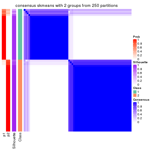
consensus_heatmap(res, k = 3)
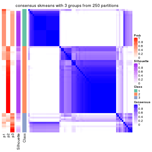
consensus_heatmap(res, k = 4)
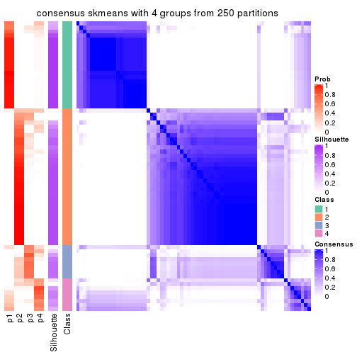
consensus_heatmap(res, k = 5)
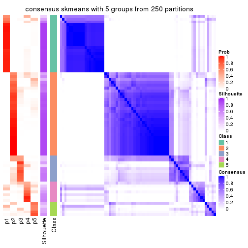
consensus_heatmap(res, k = 6)
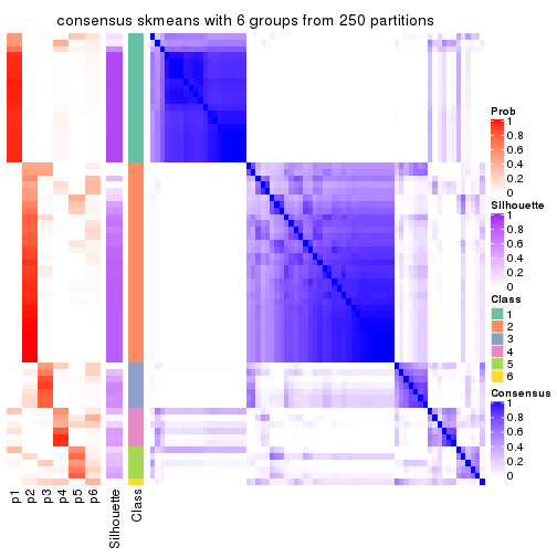
Heatmaps for the membership of samples in all partitions to see how consistent they are:
membership_heatmap(res, k = 2)
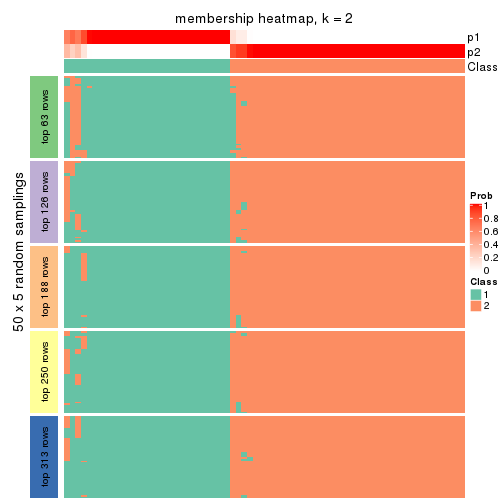
membership_heatmap(res, k = 3)
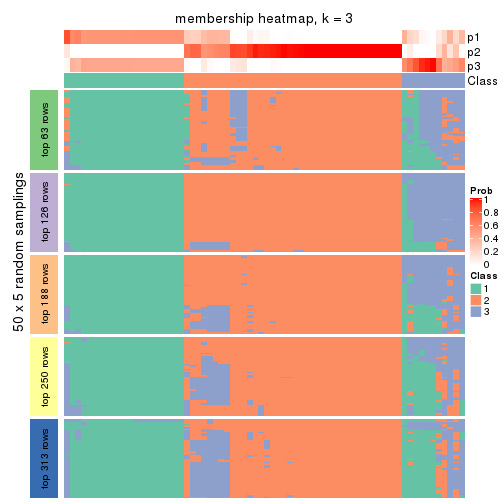
membership_heatmap(res, k = 4)
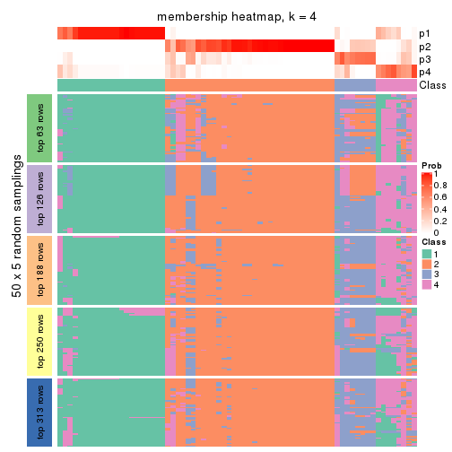
membership_heatmap(res, k = 5)
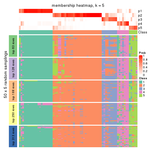
membership_heatmap(res, k = 6)
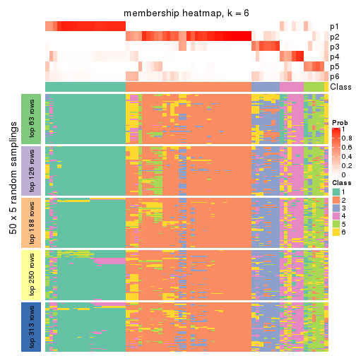
As soon as we have had the classes for columns, we can look for signatures which are significantly different between classes which can be candidate marks for certain classes. Following are the heatmaps for signatures.
Signature heatmaps where rows are scaled:
get_signatures(res, k = 2)
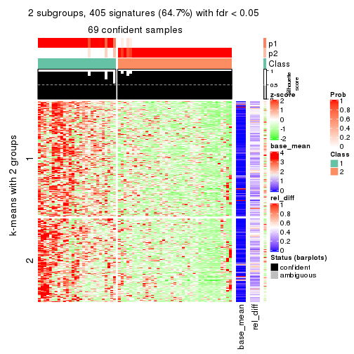
get_signatures(res, k = 3)
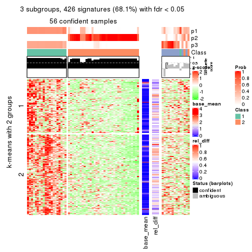
get_signatures(res, k = 4)
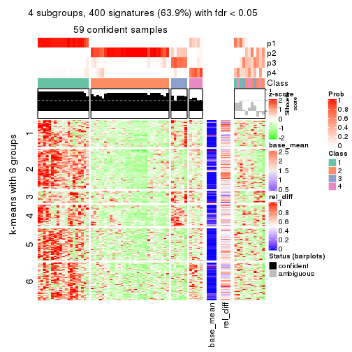
get_signatures(res, k = 5)
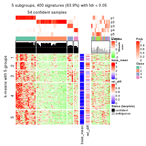
get_signatures(res, k = 6)
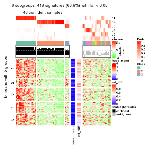
Signature heatmaps where rows are not scaled:
get_signatures(res, k = 2, scale_rows = FALSE)

get_signatures(res, k = 3, scale_rows = FALSE)
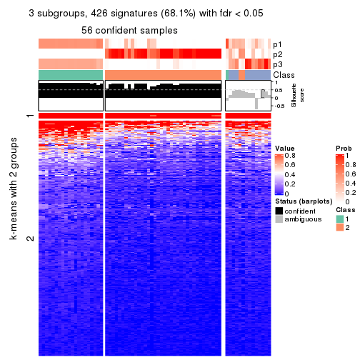
get_signatures(res, k = 4, scale_rows = FALSE)
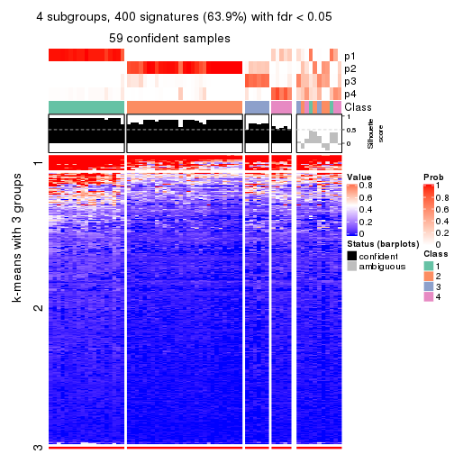
get_signatures(res, k = 5, scale_rows = FALSE)
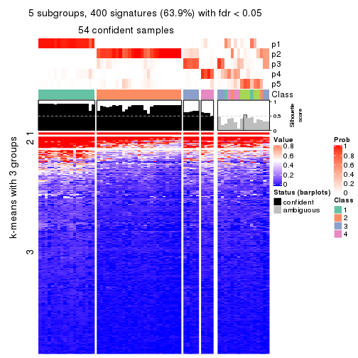
get_signatures(res, k = 6, scale_rows = FALSE)
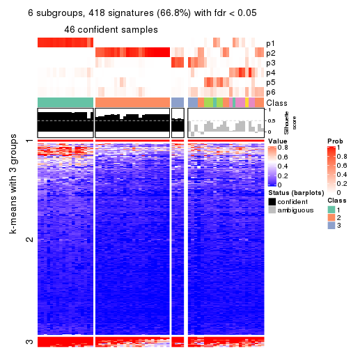
Compare the overlap of signatures from different k:
compare_signatures(res)
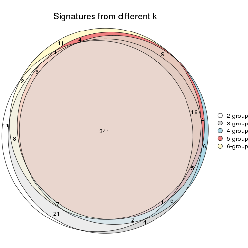
get_signature() returns a data frame invisibly. TO get the list of signatures, the function
call should be assigned to a variable explicitly. In following code, if plot argument is set
to FALSE, no heatmap is plotted while only the differential analysis is performed.
# code only for demonstration
tb = get_signature(res, k = ..., plot = FALSE)
An example of the output of tb is:
#> which_row fdr mean_1 mean_2 scaled_mean_1 scaled_mean_2 km
#> 1 38 0.042760348 8.373488 9.131774 -0.5533452 0.5164555 1
#> 2 40 0.018707592 7.106213 8.469186 -0.6173731 0.5762149 1
#> 3 55 0.019134737 10.221463 11.207825 -0.6159697 0.5749050 1
#> 4 59 0.006059896 5.921854 7.869574 -0.6899429 0.6439467 1
#> 5 60 0.018055526 8.928898 10.211722 -0.6204761 0.5791110 1
#> 6 98 0.009384629 15.714769 14.887706 0.6635654 -0.6193277 2
...
The columns in tb are:
which_row: row indices corresponding to the input matrix.fdr: FDR for the differential test. mean_x: The mean value in group x.scaled_mean_x: The mean value in group x after rows are scaled.km: Row groups if k-means clustering is applied to rows.UMAP plot which shows how samples are separated.
dimension_reduction(res, k = 2, method = "UMAP")
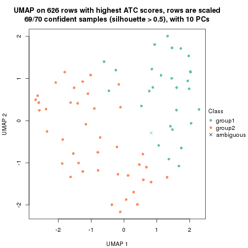
dimension_reduction(res, k = 3, method = "UMAP")
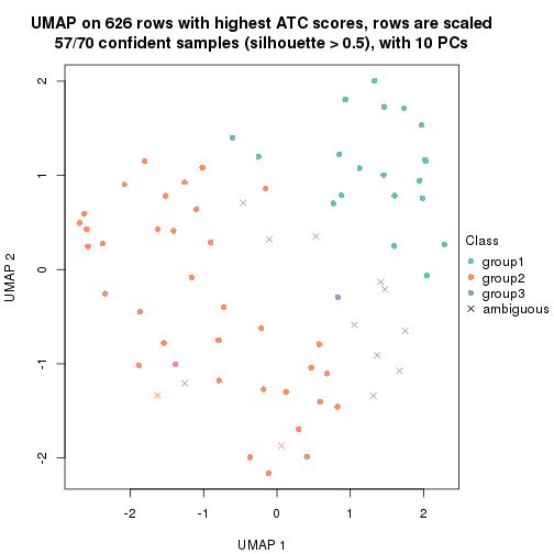
dimension_reduction(res, k = 4, method = "UMAP")
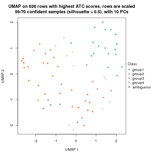
dimension_reduction(res, k = 5, method = "UMAP")
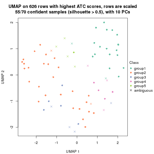
dimension_reduction(res, k = 6, method = "UMAP")
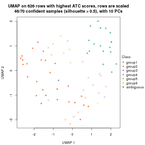
Following heatmap shows how subgroups are split when increasing k:
collect_classes(res)
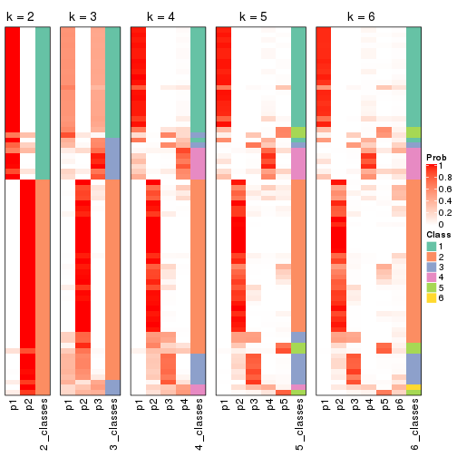
If matrix rows can be associated to genes, consider to use functional_enrichment(res,
...) to perform function enrichment for the signature genes. See this vignette for more detailed explanations.
The object with results only for a single top-value method and a single partition method can be extracted as:
res = res_list["ATC", "pam"]
# you can also extract it by
# res = res_list["ATC:pam"]
A summary of res and all the functions that can be applied to it:
res
#> A 'ConsensusPartition' object with k = 2, 3, 4, 5, 6.
#> On a matrix with 626 rows and 70 columns.
#> Top rows (63, 126, 188, 250, 313) are extracted by 'ATC' method.
#> Subgroups are detected by 'pam' method.
#> Performed in total 1250 partitions by row resampling.
#> Best k for subgroups seems to be 2.
#>
#> Following methods can be applied to this 'ConsensusPartition' object:
#> [1] "cola_report" "collect_classes" "collect_plots"
#> [4] "collect_stats" "colnames" "compare_signatures"
#> [7] "consensus_heatmap" "dimension_reduction" "functional_enrichment"
#> [10] "get_anno_col" "get_anno" "get_classes"
#> [13] "get_consensus" "get_matrix" "get_membership"
#> [16] "get_param" "get_signatures" "get_stats"
#> [19] "is_best_k" "is_stable_k" "membership_heatmap"
#> [22] "ncol" "nrow" "plot_ecdf"
#> [25] "rownames" "select_partition_number" "show"
#> [28] "suggest_best_k" "test_to_known_factors"
collect_plots() function collects all the plots made from res for all k (number of partitions)
into one single page to provide an easy and fast comparison between different k.
collect_plots(res)
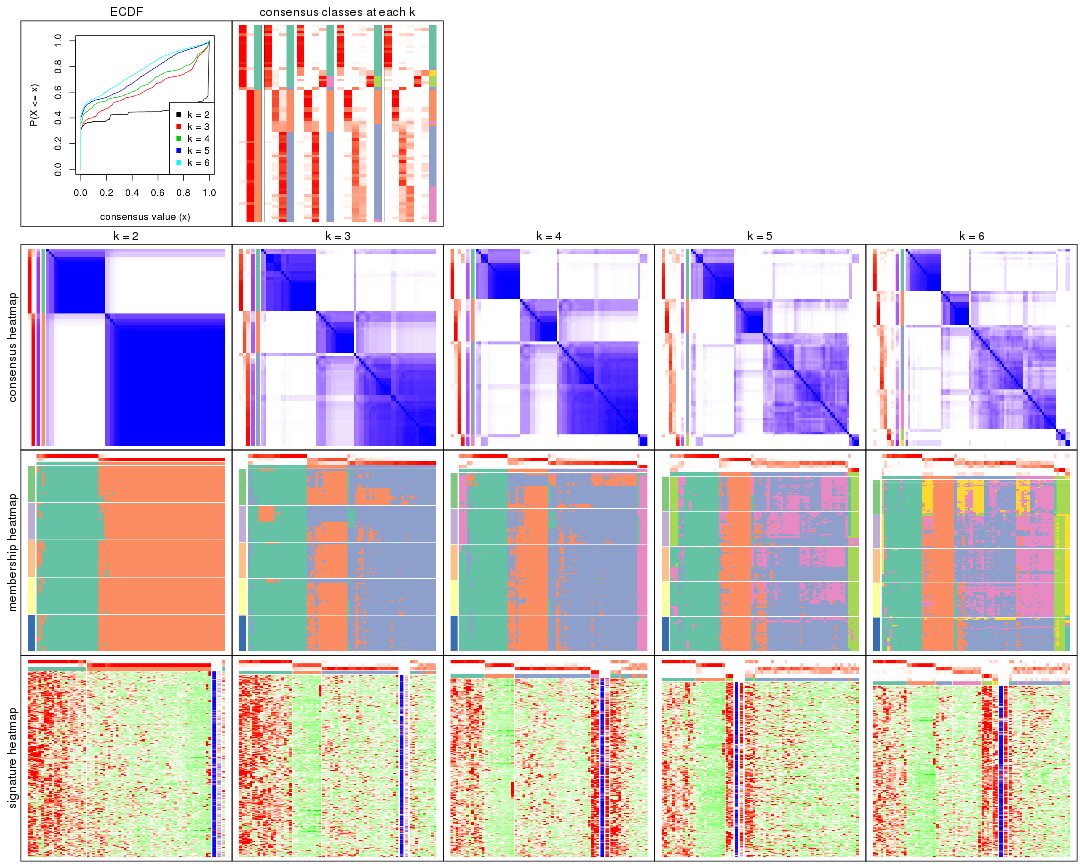
The plots are:
k and the heatmap of
predicted classes for each k.k.k.k.All the plots in panels can be made by individual functions and they are plotted later in this section.
select_partition_number() produces several plots showing different
statistics for choosing “optimized” k. There are following statistics:
k;k, the area increased is defined as \(A_k - A_{k-1}\).The detailed explanations of these statistics can be found in the cola vignette.
Generally speaking, lower PAC score, higher mean silhouette score or higher
concordance corresponds to better partition. Rand index and Jaccard index
measure how similar the current partition is compared to partition with k-1.
If they are too similar, we won't accept k is better than k-1.
select_partition_number(res)
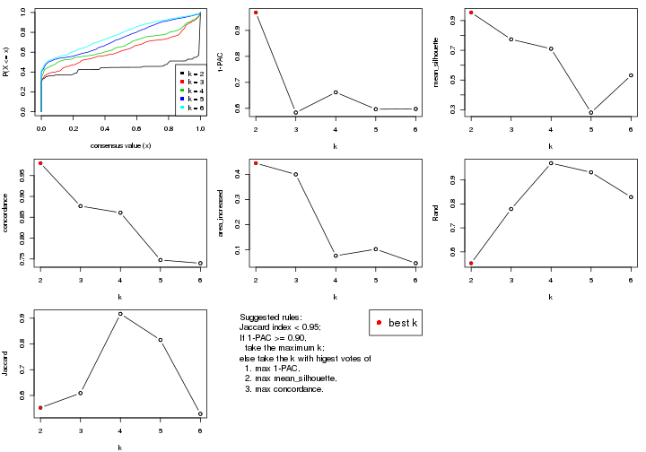
The numeric values for all these statistics can be obtained by get_stats().
get_stats(res)
#> k 1-PAC mean_silhouette concordance area_increased Rand Jaccard
#> 2 2 0.969 0.954 0.980 0.4441 0.552 0.552
#> 3 3 0.584 0.774 0.877 0.3996 0.779 0.609
#> 4 4 0.662 0.710 0.861 0.0764 0.970 0.917
#> 5 5 0.597 0.281 0.747 0.1024 0.932 0.815
#> 6 6 0.598 0.532 0.740 0.0465 0.829 0.528
suggest_best_k() suggests the best \(k\) based on these statistics. The rules are as follows:
suggest_best_k(res)
#> [1] 2
Following shows the table of the partitions (You need to click the show/hide
code output link to see it). The membership matrix (columns with name p*)
is inferred by
clue::cl_consensus()
function with the SE method. Basically the value in the membership matrix
represents the probability to belong to a certain group. The finall class
label for an item is determined with the group with highest probability it
belongs to.
In get_classes() function, the entropy is calculated from the membership
matrix and the silhouette score is calculated from the consensus matrix.
cbind(get_classes(res, k = 2), get_membership(res, k = 2))
#> class entropy silhouette p1 p2
#> SRR837437 2 0.0000 0.987 0.000 1.000
#> SRR837438 1 0.0000 0.960 1.000 0.000
#> SRR837439 2 0.0000 0.987 0.000 1.000
#> SRR837440 2 0.0000 0.987 0.000 1.000
#> SRR837441 2 0.0000 0.987 0.000 1.000
#> SRR837442 2 0.0000 0.987 0.000 1.000
#> SRR837443 2 0.0000 0.987 0.000 1.000
#> SRR837444 2 0.0938 0.977 0.012 0.988
#> SRR837445 2 0.0000 0.987 0.000 1.000
#> SRR837446 2 0.0000 0.987 0.000 1.000
#> SRR837447 1 0.0000 0.960 1.000 0.000
#> SRR837448 1 0.0000 0.960 1.000 0.000
#> SRR837449 1 0.0000 0.960 1.000 0.000
#> SRR837450 1 0.0000 0.960 1.000 0.000
#> SRR837451 2 0.0000 0.987 0.000 1.000
#> SRR837452 2 0.0000 0.987 0.000 1.000
#> SRR837453 2 0.0000 0.987 0.000 1.000
#> SRR837454 2 0.0000 0.987 0.000 1.000
#> SRR837455 1 0.0000 0.960 1.000 0.000
#> SRR837456 1 0.0000 0.960 1.000 0.000
#> SRR837457 2 0.0000 0.987 0.000 1.000
#> SRR837458 1 0.0000 0.960 1.000 0.000
#> SRR837459 2 0.0000 0.987 0.000 1.000
#> SRR837460 2 0.0000 0.987 0.000 1.000
#> SRR837461 2 0.0000 0.987 0.000 1.000
#> SRR837462 2 0.7376 0.731 0.208 0.792
#> SRR837463 1 0.7815 0.707 0.768 0.232
#> SRR837464 2 0.0000 0.987 0.000 1.000
#> SRR837465 2 0.7139 0.750 0.196 0.804
#> SRR837466 1 0.0000 0.960 1.000 0.000
#> SRR837467 2 0.0000 0.987 0.000 1.000
#> SRR837468 2 0.0000 0.987 0.000 1.000
#> SRR837469 1 0.0000 0.960 1.000 0.000
#> SRR837470 1 0.0000 0.960 1.000 0.000
#> SRR837471 2 0.0000 0.987 0.000 1.000
#> SRR837472 2 0.0000 0.987 0.000 1.000
#> SRR837473 1 0.0672 0.954 0.992 0.008
#> SRR837474 2 0.0000 0.987 0.000 1.000
#> SRR837475 2 0.0000 0.987 0.000 1.000
#> SRR837476 2 0.0000 0.987 0.000 1.000
#> SRR837477 2 0.2603 0.946 0.044 0.956
#> SRR837478 2 0.0000 0.987 0.000 1.000
#> SRR837479 2 0.0000 0.987 0.000 1.000
#> SRR837480 2 0.0000 0.987 0.000 1.000
#> SRR837481 2 0.0000 0.987 0.000 1.000
#> SRR837482 2 0.0000 0.987 0.000 1.000
#> SRR837483 1 0.0000 0.960 1.000 0.000
#> SRR837484 2 0.0000 0.987 0.000 1.000
#> SRR837485 2 0.0000 0.987 0.000 1.000
#> SRR837486 2 0.0000 0.987 0.000 1.000
#> SRR837487 2 0.0000 0.987 0.000 1.000
#> SRR837488 2 0.0000 0.987 0.000 1.000
#> SRR837489 2 0.0000 0.987 0.000 1.000
#> SRR837490 2 0.0000 0.987 0.000 1.000
#> SRR837491 2 0.4161 0.903 0.084 0.916
#> SRR837492 1 0.9491 0.437 0.632 0.368
#> SRR837493 1 0.7815 0.708 0.768 0.232
#> SRR837494 2 0.0000 0.987 0.000 1.000
#> SRR837495 2 0.0672 0.981 0.008 0.992
#> SRR837496 1 0.0000 0.960 1.000 0.000
#> SRR837497 1 0.0000 0.960 1.000 0.000
#> SRR837498 1 0.0000 0.960 1.000 0.000
#> SRR837499 1 0.0000 0.960 1.000 0.000
#> SRR837500 1 0.0000 0.960 1.000 0.000
#> SRR837501 2 0.0000 0.987 0.000 1.000
#> SRR837502 1 0.1843 0.939 0.972 0.028
#> SRR837503 1 0.0000 0.960 1.000 0.000
#> SRR837504 2 0.0000 0.987 0.000 1.000
#> SRR837505 2 0.0000 0.987 0.000 1.000
#> SRR837506 2 0.0000 0.987 0.000 1.000
cbind(get_classes(res, k = 3), get_membership(res, k = 3))
#> class entropy silhouette p1 p2 p3
#> SRR837437 2 0.6260 0.391 0.000 0.552 0.448
#> SRR837438 1 0.1529 0.906 0.960 0.000 0.040
#> SRR837439 3 0.0237 0.854 0.000 0.004 0.996
#> SRR837440 3 0.1031 0.856 0.000 0.024 0.976
#> SRR837441 3 0.0237 0.854 0.000 0.004 0.996
#> SRR837442 3 0.5785 0.407 0.000 0.332 0.668
#> SRR837443 3 0.3551 0.794 0.000 0.132 0.868
#> SRR837444 3 0.0237 0.851 0.004 0.000 0.996
#> SRR837445 3 0.0000 0.852 0.000 0.000 1.000
#> SRR837446 3 0.2959 0.829 0.000 0.100 0.900
#> SRR837447 1 0.2711 0.902 0.912 0.088 0.000
#> SRR837448 1 0.3412 0.888 0.876 0.124 0.000
#> SRR837449 1 0.0000 0.925 1.000 0.000 0.000
#> SRR837450 1 0.1860 0.914 0.948 0.052 0.000
#> SRR837451 2 0.3412 0.832 0.000 0.876 0.124
#> SRR837452 3 0.1964 0.842 0.000 0.056 0.944
#> SRR837453 2 0.3412 0.832 0.000 0.876 0.124
#> SRR837454 2 0.4291 0.811 0.000 0.820 0.180
#> SRR837455 1 0.2878 0.899 0.904 0.096 0.000
#> SRR837456 1 0.2959 0.898 0.900 0.100 0.000
#> SRR837457 2 0.3412 0.832 0.000 0.876 0.124
#> SRR837458 1 0.3412 0.888 0.876 0.124 0.000
#> SRR837459 2 0.3412 0.832 0.000 0.876 0.124
#> SRR837460 2 0.3412 0.832 0.000 0.876 0.124
#> SRR837461 3 0.3412 0.807 0.000 0.124 0.876
#> SRR837462 3 0.2959 0.753 0.100 0.000 0.900
#> SRR837463 1 0.5882 0.498 0.652 0.000 0.348
#> SRR837464 3 0.0237 0.854 0.000 0.004 0.996
#> SRR837465 3 0.2959 0.754 0.100 0.000 0.900
#> SRR837466 1 0.3412 0.888 0.876 0.124 0.000
#> SRR837467 3 0.4399 0.734 0.000 0.188 0.812
#> SRR837468 3 0.0000 0.852 0.000 0.000 1.000
#> SRR837469 1 0.0000 0.925 1.000 0.000 0.000
#> SRR837470 1 0.0000 0.925 1.000 0.000 0.000
#> SRR837471 3 0.0747 0.856 0.000 0.016 0.984
#> SRR837472 3 0.3192 0.798 0.000 0.112 0.888
#> SRR837473 1 0.0747 0.919 0.984 0.000 0.016
#> SRR837474 3 0.0892 0.856 0.000 0.020 0.980
#> SRR837475 3 0.6244 -0.103 0.000 0.440 0.560
#> SRR837476 3 0.2448 0.845 0.000 0.076 0.924
#> SRR837477 3 0.1337 0.853 0.016 0.012 0.972
#> SRR837478 2 0.6308 0.277 0.000 0.508 0.492
#> SRR837479 3 0.3038 0.825 0.000 0.104 0.896
#> SRR837480 3 0.2796 0.833 0.000 0.092 0.908
#> SRR837481 3 0.2796 0.832 0.000 0.092 0.908
#> SRR837482 3 0.0747 0.856 0.000 0.016 0.984
#> SRR837483 1 0.0000 0.925 1.000 0.000 0.000
#> SRR837484 2 0.5058 0.771 0.000 0.756 0.244
#> SRR837485 2 0.5058 0.770 0.000 0.756 0.244
#> SRR837486 3 0.2878 0.830 0.000 0.096 0.904
#> SRR837487 2 0.6305 0.333 0.000 0.516 0.484
#> SRR837488 2 0.3412 0.832 0.000 0.876 0.124
#> SRR837489 3 0.4504 0.712 0.000 0.196 0.804
#> SRR837490 2 0.6309 0.286 0.000 0.504 0.496
#> SRR837491 3 0.0747 0.846 0.016 0.000 0.984
#> SRR837492 3 0.6204 0.225 0.424 0.000 0.576
#> SRR837493 1 0.6180 0.310 0.584 0.000 0.416
#> SRR837494 2 0.3482 0.831 0.000 0.872 0.128
#> SRR837495 3 0.0237 0.853 0.004 0.000 0.996
#> SRR837496 1 0.0000 0.925 1.000 0.000 0.000
#> SRR837497 1 0.0000 0.925 1.000 0.000 0.000
#> SRR837498 1 0.0000 0.925 1.000 0.000 0.000
#> SRR837499 1 0.0000 0.925 1.000 0.000 0.000
#> SRR837500 1 0.0000 0.925 1.000 0.000 0.000
#> SRR837501 3 0.1753 0.852 0.000 0.048 0.952
#> SRR837502 1 0.2066 0.890 0.940 0.000 0.060
#> SRR837503 1 0.0000 0.925 1.000 0.000 0.000
#> SRR837504 3 0.3340 0.814 0.000 0.120 0.880
#> SRR837505 3 0.5926 0.344 0.000 0.356 0.644
#> SRR837506 2 0.3879 0.825 0.000 0.848 0.152
cbind(get_classes(res, k = 4), get_membership(res, k = 4))
#> class entropy silhouette p1 p2 p3 p4
#> SRR837437 2 0.5250 0.2262 0.000 0.552 0.440 0.008
#> SRR837438 1 0.1209 0.8067 0.964 0.000 0.032 0.004
#> SRR837439 3 0.0657 0.8689 0.000 0.012 0.984 0.004
#> SRR837440 3 0.1209 0.8702 0.000 0.032 0.964 0.004
#> SRR837441 3 0.0524 0.8681 0.000 0.008 0.988 0.004
#> SRR837442 3 0.4917 0.4784 0.000 0.336 0.656 0.008
#> SRR837443 3 0.3271 0.8163 0.000 0.132 0.856 0.012
#> SRR837444 3 0.0188 0.8655 0.000 0.000 0.996 0.004
#> SRR837445 3 0.0188 0.8655 0.000 0.000 0.996 0.004
#> SRR837446 3 0.2741 0.8465 0.000 0.096 0.892 0.012
#> SRR837447 1 0.4730 0.4038 0.636 0.000 0.000 0.364
#> SRR837448 4 0.0469 0.8530 0.012 0.000 0.000 0.988
#> SRR837449 1 0.0000 0.8292 1.000 0.000 0.000 0.000
#> SRR837450 4 0.4817 0.3581 0.388 0.000 0.000 0.612
#> SRR837451 2 0.0000 0.7332 0.000 1.000 0.000 0.000
#> SRR837452 3 0.1637 0.8590 0.000 0.060 0.940 0.000
#> SRR837453 2 0.0000 0.7332 0.000 1.000 0.000 0.000
#> SRR837454 2 0.1637 0.7189 0.000 0.940 0.060 0.000
#> SRR837455 1 0.4830 0.3508 0.608 0.000 0.000 0.392
#> SRR837456 1 0.4925 0.2683 0.572 0.000 0.000 0.428
#> SRR837457 2 0.0000 0.7332 0.000 1.000 0.000 0.000
#> SRR837458 4 0.0469 0.8530 0.012 0.000 0.000 0.988
#> SRR837459 2 0.0000 0.7332 0.000 1.000 0.000 0.000
#> SRR837460 2 0.0000 0.7332 0.000 1.000 0.000 0.000
#> SRR837461 3 0.2944 0.8285 0.000 0.128 0.868 0.004
#> SRR837462 3 0.2401 0.7962 0.092 0.000 0.904 0.004
#> SRR837463 1 0.4819 0.3878 0.652 0.000 0.344 0.004
#> SRR837464 3 0.0188 0.8675 0.000 0.004 0.996 0.000
#> SRR837465 3 0.2334 0.8004 0.088 0.000 0.908 0.004
#> SRR837466 4 0.0469 0.8530 0.012 0.000 0.000 0.988
#> SRR837467 3 0.3893 0.7523 0.000 0.196 0.796 0.008
#> SRR837468 3 0.0000 0.8661 0.000 0.000 1.000 0.000
#> SRR837469 1 0.0000 0.8292 1.000 0.000 0.000 0.000
#> SRR837470 1 0.0188 0.8274 0.996 0.000 0.000 0.004
#> SRR837471 3 0.0469 0.8687 0.000 0.012 0.988 0.000
#> SRR837472 3 0.2469 0.8201 0.000 0.108 0.892 0.000
#> SRR837473 1 0.0592 0.8186 0.984 0.000 0.016 0.000
#> SRR837474 3 0.0779 0.8701 0.000 0.016 0.980 0.004
#> SRR837475 3 0.5132 0.0536 0.000 0.448 0.548 0.004
#> SRR837476 3 0.1867 0.8632 0.000 0.072 0.928 0.000
#> SRR837477 3 0.0779 0.8658 0.016 0.004 0.980 0.000
#> SRR837478 2 0.5277 0.1790 0.000 0.532 0.460 0.008
#> SRR837479 3 0.2737 0.8402 0.000 0.104 0.888 0.008
#> SRR837480 3 0.2401 0.8496 0.000 0.092 0.904 0.004
#> SRR837481 3 0.2412 0.8502 0.000 0.084 0.908 0.008
#> SRR837482 3 0.0336 0.8689 0.000 0.008 0.992 0.000
#> SRR837483 1 0.0000 0.8292 1.000 0.000 0.000 0.000
#> SRR837484 2 0.4086 0.6755 0.000 0.776 0.216 0.008
#> SRR837485 2 0.3933 0.6835 0.000 0.792 0.200 0.008
#> SRR837486 3 0.2546 0.8460 0.000 0.092 0.900 0.008
#> SRR837487 2 0.5277 0.2101 0.000 0.532 0.460 0.008
#> SRR837488 2 0.0000 0.7332 0.000 1.000 0.000 0.000
#> SRR837489 3 0.3852 0.7449 0.000 0.192 0.800 0.008
#> SRR837490 2 0.5277 0.2100 0.000 0.532 0.460 0.008
#> SRR837491 3 0.0779 0.8625 0.016 0.000 0.980 0.004
#> SRR837492 3 0.4907 0.2264 0.420 0.000 0.580 0.000
#> SRR837493 1 0.5088 0.2737 0.572 0.000 0.424 0.004
#> SRR837494 2 0.0336 0.7349 0.000 0.992 0.008 0.000
#> SRR837495 3 0.0376 0.8657 0.004 0.000 0.992 0.004
#> SRR837496 1 0.0000 0.8292 1.000 0.000 0.000 0.000
#> SRR837497 1 0.0000 0.8292 1.000 0.000 0.000 0.000
#> SRR837498 1 0.0000 0.8292 1.000 0.000 0.000 0.000
#> SRR837499 1 0.0000 0.8292 1.000 0.000 0.000 0.000
#> SRR837500 1 0.0000 0.8292 1.000 0.000 0.000 0.000
#> SRR837501 3 0.1302 0.8691 0.000 0.044 0.956 0.000
#> SRR837502 1 0.1637 0.7832 0.940 0.000 0.060 0.000
#> SRR837503 1 0.0188 0.8278 0.996 0.000 0.000 0.004
#> SRR837504 3 0.2976 0.8341 0.000 0.120 0.872 0.008
#> SRR837505 3 0.5040 0.4179 0.000 0.364 0.628 0.008
#> SRR837506 2 0.2197 0.7254 0.000 0.916 0.080 0.004
cbind(get_classes(res, k = 5), get_membership(res, k = 5))
#> class entropy silhouette p1 p2 p3 p4 p5
#> SRR837437 2 0.6802 -0.2605 0.000 0.356 0.292 0.352 0.000
#> SRR837438 1 0.1522 0.7658 0.944 0.000 0.012 0.044 0.000
#> SRR837439 3 0.4304 -0.6541 0.000 0.000 0.516 0.484 0.000
#> SRR837440 3 0.4294 -0.5710 0.000 0.000 0.532 0.468 0.000
#> SRR837441 3 0.4302 -0.6292 0.000 0.000 0.520 0.480 0.000
#> SRR837442 3 0.5927 -0.1274 0.000 0.104 0.468 0.428 0.000
#> SRR837443 3 0.4659 -0.4215 0.000 0.012 0.496 0.492 0.000
#> SRR837444 4 0.4307 0.0000 0.000 0.000 0.496 0.504 0.000
#> SRR837445 3 0.3707 -0.2181 0.000 0.000 0.716 0.284 0.000
#> SRR837446 3 0.3983 -0.1634 0.000 0.000 0.660 0.340 0.000
#> SRR837447 1 0.5975 0.2378 0.532 0.000 0.000 0.124 0.344
#> SRR837448 5 0.0000 0.8372 0.000 0.000 0.000 0.000 1.000
#> SRR837449 1 0.0000 0.7923 1.000 0.000 0.000 0.000 0.000
#> SRR837450 5 0.4416 0.3872 0.356 0.000 0.000 0.012 0.632
#> SRR837451 2 0.0000 0.8150 0.000 1.000 0.000 0.000 0.000
#> SRR837452 3 0.1082 0.2697 0.000 0.028 0.964 0.008 0.000
#> SRR837453 2 0.0000 0.8150 0.000 1.000 0.000 0.000 0.000
#> SRR837454 2 0.1251 0.7944 0.000 0.956 0.036 0.008 0.000
#> SRR837455 1 0.6498 0.0849 0.452 0.000 0.000 0.196 0.352
#> SRR837456 1 0.6527 0.0164 0.428 0.000 0.000 0.196 0.376
#> SRR837457 2 0.0000 0.8150 0.000 1.000 0.000 0.000 0.000
#> SRR837458 5 0.1965 0.8140 0.000 0.000 0.000 0.096 0.904
#> SRR837459 2 0.0000 0.8150 0.000 1.000 0.000 0.000 0.000
#> SRR837460 2 0.0000 0.8150 0.000 1.000 0.000 0.000 0.000
#> SRR837461 3 0.5296 -0.5253 0.000 0.048 0.484 0.468 0.000
#> SRR837462 3 0.3909 -0.0124 0.024 0.000 0.760 0.216 0.000
#> SRR837463 1 0.6141 0.3098 0.560 0.000 0.196 0.244 0.000
#> SRR837464 3 0.3305 -0.1248 0.000 0.000 0.776 0.224 0.000
#> SRR837465 3 0.4878 -0.7102 0.024 0.000 0.536 0.440 0.000
#> SRR837466 5 0.0000 0.8372 0.000 0.000 0.000 0.000 1.000
#> SRR837467 3 0.5484 -0.1981 0.000 0.068 0.540 0.392 0.000
#> SRR837468 3 0.3003 -0.0192 0.000 0.000 0.812 0.188 0.000
#> SRR837469 1 0.0290 0.7915 0.992 0.000 0.000 0.008 0.000
#> SRR837470 1 0.0324 0.7911 0.992 0.000 0.000 0.004 0.004
#> SRR837471 3 0.2439 0.1805 0.000 0.004 0.876 0.120 0.000
#> SRR837472 3 0.3303 0.2443 0.000 0.076 0.848 0.076 0.000
#> SRR837473 1 0.1012 0.7818 0.968 0.000 0.012 0.020 0.000
#> SRR837474 3 0.4101 -0.5233 0.000 0.000 0.628 0.372 0.000
#> SRR837475 3 0.5491 0.2310 0.000 0.312 0.600 0.088 0.000
#> SRR837476 3 0.3897 0.1173 0.000 0.028 0.768 0.204 0.000
#> SRR837477 3 0.2020 0.2339 0.000 0.000 0.900 0.100 0.000
#> SRR837478 3 0.6215 0.2028 0.000 0.348 0.500 0.152 0.000
#> SRR837479 3 0.3596 0.2314 0.000 0.012 0.776 0.212 0.000
#> SRR837480 3 0.3424 0.1939 0.000 0.000 0.760 0.240 0.000
#> SRR837481 3 0.2813 0.2631 0.000 0.000 0.832 0.168 0.000
#> SRR837482 3 0.2280 0.2245 0.000 0.000 0.880 0.120 0.000
#> SRR837483 1 0.1341 0.7657 0.944 0.000 0.000 0.056 0.000
#> SRR837484 2 0.5440 0.5804 0.000 0.660 0.184 0.156 0.000
#> SRR837485 2 0.5452 0.5580 0.000 0.656 0.200 0.144 0.000
#> SRR837486 3 0.4060 -0.0082 0.000 0.000 0.640 0.360 0.000
#> SRR837487 3 0.6499 0.0368 0.000 0.396 0.416 0.188 0.000
#> SRR837488 2 0.0000 0.8150 0.000 1.000 0.000 0.000 0.000
#> SRR837489 3 0.3780 0.2880 0.000 0.072 0.812 0.116 0.000
#> SRR837490 3 0.5490 0.2315 0.000 0.324 0.592 0.084 0.000
#> SRR837491 3 0.2777 0.1740 0.016 0.000 0.864 0.120 0.000
#> SRR837492 3 0.5060 0.1133 0.224 0.000 0.684 0.092 0.000
#> SRR837493 1 0.6428 0.1232 0.456 0.000 0.364 0.180 0.000
#> SRR837494 2 0.0771 0.8092 0.000 0.976 0.004 0.020 0.000
#> SRR837495 3 0.3010 0.1353 0.004 0.000 0.824 0.172 0.000
#> SRR837496 1 0.0000 0.7923 1.000 0.000 0.000 0.000 0.000
#> SRR837497 1 0.0963 0.7797 0.964 0.000 0.000 0.036 0.000
#> SRR837498 1 0.0000 0.7923 1.000 0.000 0.000 0.000 0.000
#> SRR837499 1 0.0000 0.7923 1.000 0.000 0.000 0.000 0.000
#> SRR837500 1 0.0000 0.7923 1.000 0.000 0.000 0.000 0.000
#> SRR837501 3 0.4470 -0.3884 0.000 0.012 0.616 0.372 0.000
#> SRR837502 1 0.2124 0.7406 0.916 0.000 0.056 0.028 0.000
#> SRR837503 1 0.0162 0.7919 0.996 0.000 0.000 0.000 0.004
#> SRR837504 3 0.4437 -0.3146 0.000 0.004 0.532 0.464 0.000
#> SRR837505 3 0.6507 0.0171 0.000 0.212 0.472 0.316 0.000
#> SRR837506 2 0.3593 0.7305 0.000 0.828 0.084 0.088 0.000
cbind(get_classes(res, k = 6), get_membership(res, k = 6))
#> class entropy silhouette p1 p2 p3 p4 p5 p6
#> SRR837437 4 0.7419 0.2893 0.000 0.228 0.188 0.400 0.000 0.184
#> SRR837438 1 0.1398 0.8183 0.940 0.000 0.008 0.052 0.000 0.000
#> SRR837439 4 0.3101 0.6941 0.000 0.000 0.244 0.756 0.000 0.000
#> SRR837440 4 0.3244 0.7004 0.000 0.000 0.268 0.732 0.000 0.000
#> SRR837441 4 0.3076 0.6946 0.000 0.000 0.240 0.760 0.000 0.000
#> SRR837442 4 0.6350 0.5438 0.000 0.048 0.272 0.516 0.000 0.164
#> SRR837443 4 0.3290 0.7024 0.000 0.000 0.252 0.744 0.000 0.004
#> SRR837444 4 0.3706 0.5537 0.000 0.000 0.380 0.620 0.000 0.000
#> SRR837445 3 0.3330 0.2380 0.000 0.000 0.716 0.284 0.000 0.000
#> SRR837446 3 0.4808 -0.3313 0.000 0.000 0.480 0.468 0.000 0.052
#> SRR837447 1 0.5873 -0.4964 0.444 0.000 0.000 0.000 0.204 0.352
#> SRR837448 5 0.0000 0.7452 0.000 0.000 0.000 0.000 1.000 0.000
#> SRR837449 1 0.0000 0.8521 1.000 0.000 0.000 0.000 0.000 0.000
#> SRR837450 5 0.3403 0.5060 0.212 0.000 0.000 0.000 0.768 0.020
#> SRR837451 2 0.0000 0.8183 0.000 1.000 0.000 0.000 0.000 0.000
#> SRR837452 3 0.3092 0.4866 0.000 0.028 0.840 0.120 0.000 0.012
#> SRR837453 2 0.0000 0.8183 0.000 1.000 0.000 0.000 0.000 0.000
#> SRR837454 2 0.1225 0.7950 0.000 0.952 0.036 0.012 0.000 0.000
#> SRR837455 6 0.5219 1.0000 0.176 0.000 0.000 0.000 0.212 0.612
#> SRR837456 6 0.5219 1.0000 0.176 0.000 0.000 0.000 0.212 0.612
#> SRR837457 2 0.0000 0.8183 0.000 1.000 0.000 0.000 0.000 0.000
#> SRR837458 5 0.3470 0.5170 0.000 0.000 0.000 0.012 0.740 0.248
#> SRR837459 2 0.0000 0.8183 0.000 1.000 0.000 0.000 0.000 0.000
#> SRR837460 2 0.0000 0.8183 0.000 1.000 0.000 0.000 0.000 0.000
#> SRR837461 4 0.3850 0.6999 0.000 0.020 0.260 0.716 0.000 0.004
#> SRR837462 3 0.3151 0.3725 0.000 0.000 0.748 0.252 0.000 0.000
#> SRR837463 1 0.5701 0.1851 0.524 0.000 0.228 0.248 0.000 0.000
#> SRR837464 3 0.3937 -0.1245 0.000 0.000 0.572 0.424 0.000 0.004
#> SRR837465 4 0.4091 0.3502 0.008 0.000 0.472 0.520 0.000 0.000
#> SRR837466 5 0.0000 0.7452 0.000 0.000 0.000 0.000 1.000 0.000
#> SRR837467 4 0.5609 0.6383 0.000 0.040 0.308 0.576 0.000 0.076
#> SRR837468 3 0.3620 0.1484 0.000 0.000 0.648 0.352 0.000 0.000
#> SRR837469 1 0.1074 0.8420 0.960 0.000 0.000 0.028 0.000 0.012
#> SRR837470 1 0.0777 0.8468 0.972 0.000 0.000 0.024 0.004 0.000
#> SRR837471 3 0.1411 0.5134 0.000 0.004 0.936 0.060 0.000 0.000
#> SRR837472 3 0.2488 0.5118 0.000 0.076 0.880 0.044 0.000 0.000
#> SRR837473 1 0.1088 0.8382 0.960 0.000 0.024 0.016 0.000 0.000
#> SRR837474 4 0.4229 0.5373 0.000 0.000 0.436 0.548 0.000 0.016
#> SRR837475 3 0.6587 0.3000 0.000 0.284 0.496 0.076 0.000 0.144
#> SRR837476 3 0.4621 0.0468 0.000 0.016 0.604 0.356 0.000 0.024
#> SRR837477 3 0.0405 0.5186 0.000 0.000 0.988 0.004 0.000 0.008
#> SRR837478 3 0.7338 0.0986 0.000 0.316 0.356 0.124 0.000 0.204
#> SRR837479 3 0.5579 0.2215 0.000 0.012 0.596 0.184 0.000 0.208
#> SRR837480 3 0.5416 0.1675 0.000 0.000 0.580 0.224 0.000 0.196
#> SRR837481 3 0.4672 0.3607 0.000 0.000 0.684 0.128 0.000 0.188
#> SRR837482 3 0.2006 0.5042 0.000 0.000 0.904 0.080 0.000 0.016
#> SRR837483 1 0.2826 0.7454 0.856 0.000 0.000 0.092 0.000 0.052
#> SRR837484 2 0.5680 0.6075 0.000 0.628 0.052 0.112 0.000 0.208
#> SRR837485 2 0.5904 0.5843 0.000 0.616 0.080 0.104 0.000 0.200
#> SRR837486 3 0.5873 -0.2588 0.000 0.000 0.444 0.352 0.000 0.204
#> SRR837487 2 0.7410 0.0522 0.000 0.380 0.268 0.148 0.000 0.204
#> SRR837488 2 0.0000 0.8183 0.000 1.000 0.000 0.000 0.000 0.000
#> SRR837489 3 0.5265 0.4165 0.000 0.064 0.684 0.168 0.000 0.084
#> SRR837490 3 0.6238 0.2572 0.000 0.292 0.504 0.032 0.000 0.172
#> SRR837491 3 0.1398 0.5132 0.008 0.000 0.940 0.052 0.000 0.000
#> SRR837492 3 0.2191 0.4656 0.120 0.000 0.876 0.004 0.000 0.000
#> SRR837493 3 0.5505 -0.0255 0.420 0.000 0.452 0.128 0.000 0.000
#> SRR837494 2 0.0891 0.8098 0.000 0.968 0.000 0.024 0.000 0.008
#> SRR837495 3 0.1444 0.5043 0.000 0.000 0.928 0.072 0.000 0.000
#> SRR837496 1 0.0000 0.8521 1.000 0.000 0.000 0.000 0.000 0.000
#> SRR837497 1 0.1753 0.8040 0.912 0.000 0.000 0.084 0.000 0.004
#> SRR837498 1 0.0146 0.8519 0.996 0.000 0.000 0.004 0.000 0.000
#> SRR837499 1 0.0000 0.8521 1.000 0.000 0.000 0.000 0.000 0.000
#> SRR837500 1 0.0000 0.8521 1.000 0.000 0.000 0.000 0.000 0.000
#> SRR837501 4 0.4344 0.5203 0.000 0.008 0.412 0.568 0.000 0.012
#> SRR837502 1 0.1863 0.7674 0.896 0.000 0.104 0.000 0.000 0.000
#> SRR837503 1 0.0146 0.8515 0.996 0.000 0.000 0.000 0.004 0.000
#> SRR837504 4 0.4810 0.6647 0.000 0.000 0.292 0.624 0.000 0.084
#> SRR837505 4 0.7505 0.2832 0.000 0.172 0.284 0.352 0.000 0.192
#> SRR837506 2 0.4262 0.7031 0.000 0.760 0.024 0.068 0.000 0.148
Heatmaps for the consensus matrix. It visualizes the probability of two samples to be in a same group.
consensus_heatmap(res, k = 2)
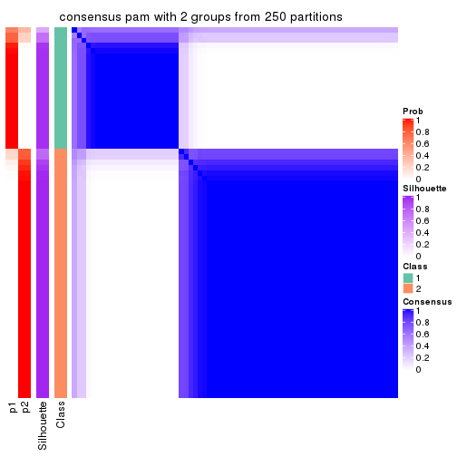
consensus_heatmap(res, k = 3)
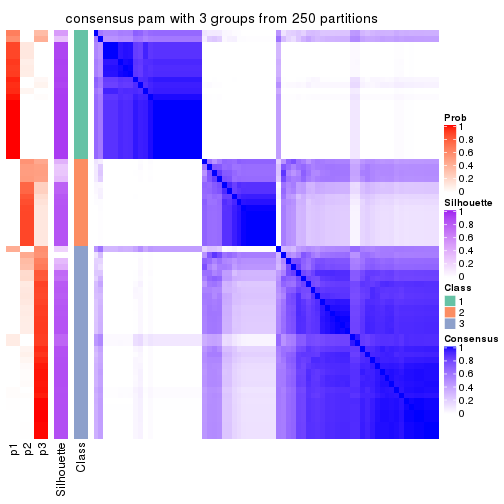
consensus_heatmap(res, k = 4)
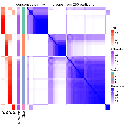
consensus_heatmap(res, k = 5)
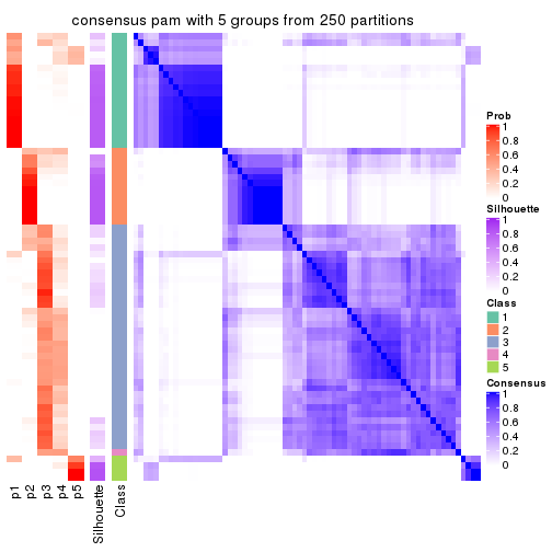
consensus_heatmap(res, k = 6)
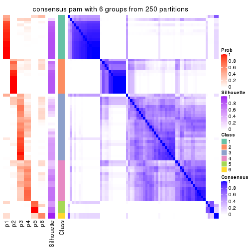
Heatmaps for the membership of samples in all partitions to see how consistent they are:
membership_heatmap(res, k = 2)
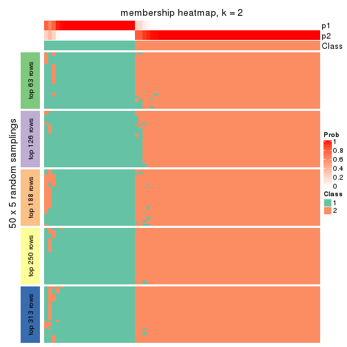
membership_heatmap(res, k = 3)
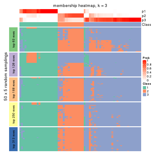
membership_heatmap(res, k = 4)
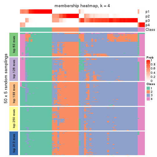
membership_heatmap(res, k = 5)
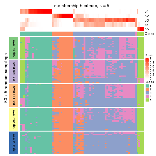
membership_heatmap(res, k = 6)
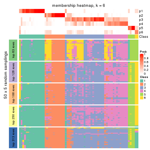
As soon as we have had the classes for columns, we can look for signatures which are significantly different between classes which can be candidate marks for certain classes. Following are the heatmaps for signatures.
Signature heatmaps where rows are scaled:
get_signatures(res, k = 2)
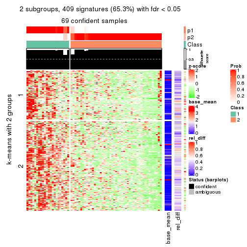
get_signatures(res, k = 3)
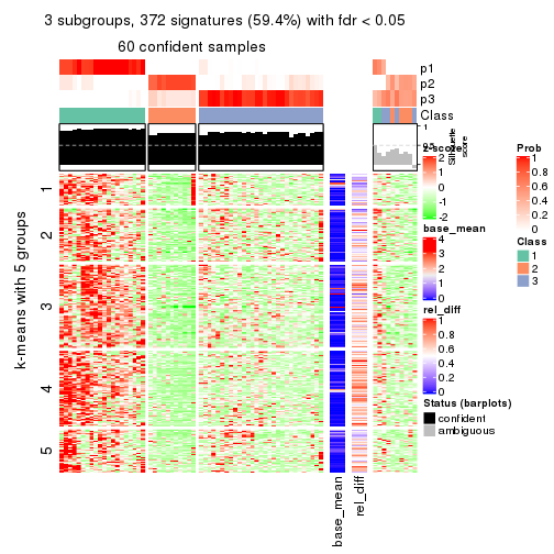
get_signatures(res, k = 4)
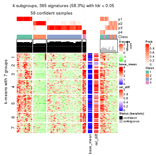
get_signatures(res, k = 5)
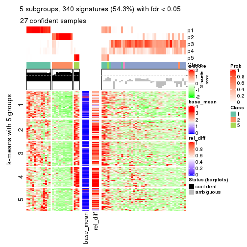
get_signatures(res, k = 6)
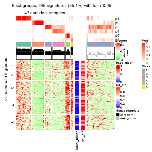
Signature heatmaps where rows are not scaled:
get_signatures(res, k = 2, scale_rows = FALSE)
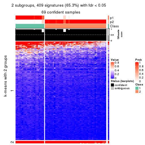
get_signatures(res, k = 3, scale_rows = FALSE)
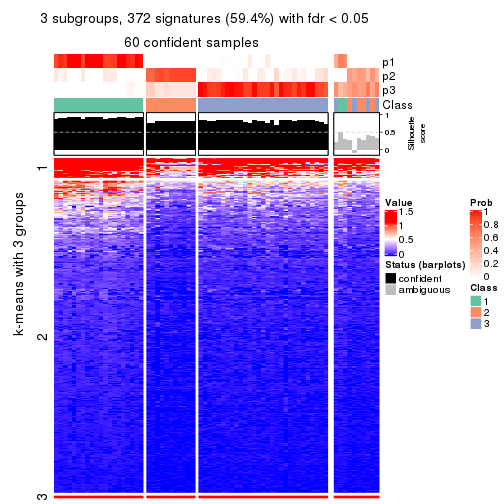
get_signatures(res, k = 4, scale_rows = FALSE)
get_signatures(res, k = 5, scale_rows = FALSE)
get_signatures(res, k = 6, scale_rows = FALSE)
Compare the overlap of signatures from different k:
compare_signatures(res)
get_signature() returns a data frame invisibly. TO get the list of signatures, the function
call should be assigned to a variable explicitly. In following code, if plot argument is set
to FALSE, no heatmap is plotted while only the differential analysis is performed.
# code only for demonstration
tb = get_signature(res, k = ..., plot = FALSE)
An example of the output of tb is:
#> which_row fdr mean_1 mean_2 scaled_mean_1 scaled_mean_2 km
#> 1 38 0.042760348 8.373488 9.131774 -0.5533452 0.5164555 1
#> 2 40 0.018707592 7.106213 8.469186 -0.6173731 0.5762149 1
#> 3 55 0.019134737 10.221463 11.207825 -0.6159697 0.5749050 1
#> 4 59 0.006059896 5.921854 7.869574 -0.6899429 0.6439467 1
#> 5 60 0.018055526 8.928898 10.211722 -0.6204761 0.5791110 1
#> 6 98 0.009384629 15.714769 14.887706 0.6635654 -0.6193277 2
...
The columns in tb are:
which_row: row indices corresponding to the input matrix.fdr: FDR for the differential test. mean_x: The mean value in group x.scaled_mean_x: The mean value in group x after rows are scaled.km: Row groups if k-means clustering is applied to rows.UMAP plot which shows how samples are separated.
dimension_reduction(res, k = 2, method = "UMAP")

dimension_reduction(res, k = 3, method = "UMAP")
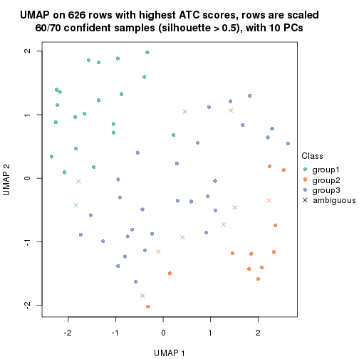
dimension_reduction(res, k = 4, method = "UMAP")
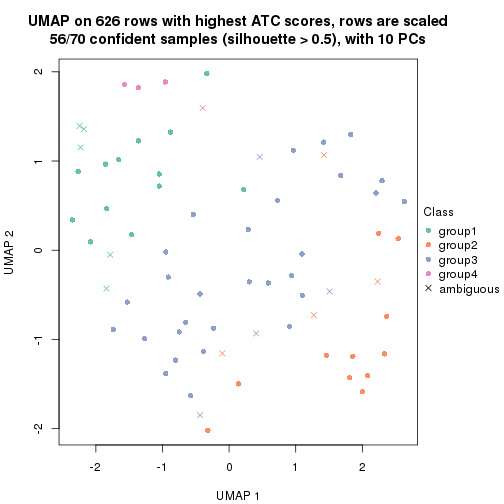
dimension_reduction(res, k = 5, method = "UMAP")
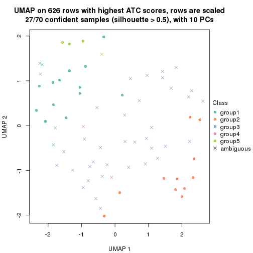
dimension_reduction(res, k = 6, method = "UMAP")
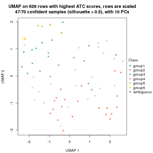
Following heatmap shows how subgroups are split when increasing k:
collect_classes(res)
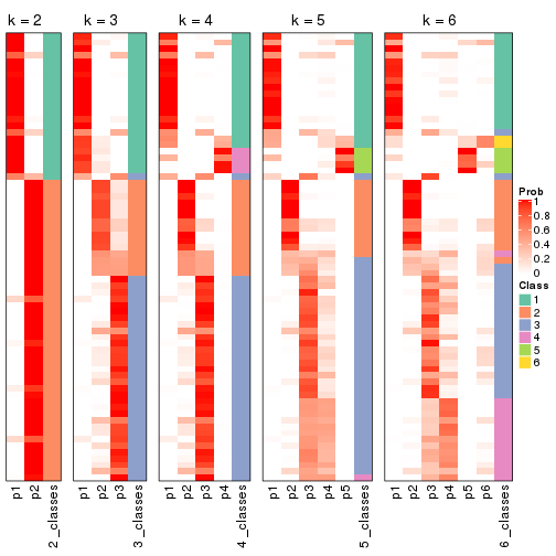
If matrix rows can be associated to genes, consider to use functional_enrichment(res,
...) to perform function enrichment for the signature genes. See this vignette for more detailed explanations.
The object with results only for a single top-value method and a single partition method can be extracted as:
res = res_list["ATC", "mclust"]
# you can also extract it by
# res = res_list["ATC:mclust"]
A summary of res and all the functions that can be applied to it:
res
#> A 'ConsensusPartition' object with k = 2, 3, 4, 5, 6.
#> On a matrix with 626 rows and 70 columns.
#> Top rows (63, 126, 188, 250, 313) are extracted by 'ATC' method.
#> Subgroups are detected by 'mclust' method.
#> Performed in total 1250 partitions by row resampling.
#> Best k for subgroups seems to be 2.
#>
#> Following methods can be applied to this 'ConsensusPartition' object:
#> [1] "cola_report" "collect_classes" "collect_plots"
#> [4] "collect_stats" "colnames" "compare_signatures"
#> [7] "consensus_heatmap" "dimension_reduction" "functional_enrichment"
#> [10] "get_anno_col" "get_anno" "get_classes"
#> [13] "get_consensus" "get_matrix" "get_membership"
#> [16] "get_param" "get_signatures" "get_stats"
#> [19] "is_best_k" "is_stable_k" "membership_heatmap"
#> [22] "ncol" "nrow" "plot_ecdf"
#> [25] "rownames" "select_partition_number" "show"
#> [28] "suggest_best_k" "test_to_known_factors"
collect_plots() function collects all the plots made from res for all k (number of partitions)
into one single page to provide an easy and fast comparison between different k.
collect_plots(res)
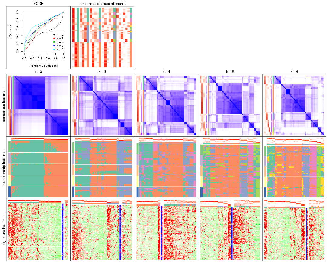
The plots are:
k and the heatmap of
predicted classes for each k.k.k.k.All the plots in panels can be made by individual functions and they are plotted later in this section.
select_partition_number() produces several plots showing different
statistics for choosing “optimized” k. There are following statistics:
k;k, the area increased is defined as \(A_k - A_{k-1}\).The detailed explanations of these statistics can be found in the cola vignette.
Generally speaking, lower PAC score, higher mean silhouette score or higher
concordance corresponds to better partition. Rand index and Jaccard index
measure how similar the current partition is compared to partition with k-1.
If they are too similar, we won't accept k is better than k-1.
select_partition_number(res)
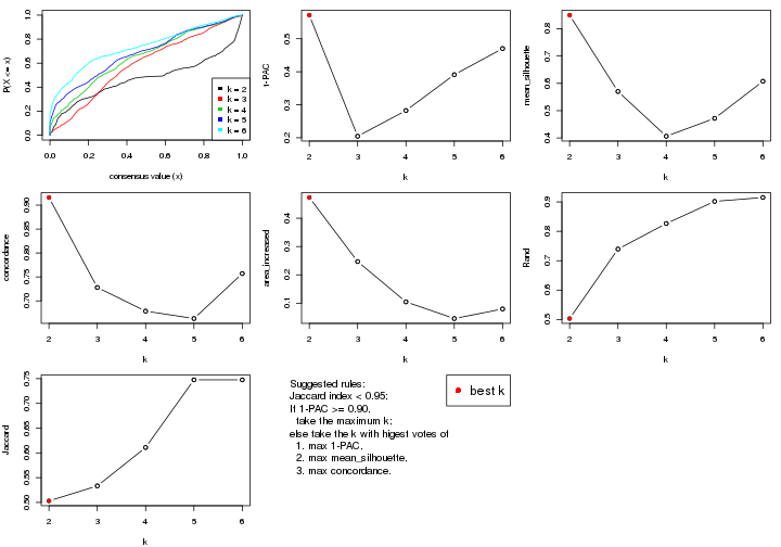
The numeric values for all these statistics can be obtained by get_stats().
get_stats(res)
#> k 1-PAC mean_silhouette concordance area_increased Rand Jaccard
#> 2 2 0.572 0.850 0.916 0.4732 0.503 0.503
#> 3 3 0.205 0.570 0.728 0.2469 0.740 0.533
#> 4 4 0.283 0.406 0.679 0.1046 0.827 0.611
#> 5 5 0.391 0.472 0.663 0.0457 0.902 0.748
#> 6 6 0.470 0.608 0.757 0.0796 0.915 0.748
suggest_best_k() suggests the best \(k\) based on these statistics. The rules are as follows:
suggest_best_k(res)
#> [1] 2
Following shows the table of the partitions (You need to click the show/hide
code output link to see it). The membership matrix (columns with name p*)
is inferred by
clue::cl_consensus()
function with the SE method. Basically the value in the membership matrix
represents the probability to belong to a certain group. The finall class
label for an item is determined with the group with highest probability it
belongs to.
In get_classes() function, the entropy is calculated from the membership
matrix and the silhouette score is calculated from the consensus matrix.
cbind(get_classes(res, k = 2), get_membership(res, k = 2))
#> class entropy silhouette p1 p2
#> SRR837437 2 0.0000 0.878 0.000 1.000
#> SRR837438 1 0.2603 0.929 0.956 0.044
#> SRR837439 1 0.7528 0.740 0.784 0.216
#> SRR837440 2 0.7674 0.775 0.224 0.776
#> SRR837441 2 0.8016 0.753 0.244 0.756
#> SRR837442 2 0.0672 0.881 0.008 0.992
#> SRR837443 2 0.4939 0.865 0.108 0.892
#> SRR837444 1 0.7299 0.752 0.796 0.204
#> SRR837445 2 0.7883 0.759 0.236 0.764
#> SRR837446 2 0.4431 0.872 0.092 0.908
#> SRR837447 1 0.0938 0.932 0.988 0.012
#> SRR837448 1 0.0000 0.928 1.000 0.000
#> SRR837449 1 0.0938 0.932 0.988 0.012
#> SRR837450 1 0.0000 0.928 1.000 0.000
#> SRR837451 2 0.0000 0.878 0.000 1.000
#> SRR837452 2 0.1633 0.883 0.024 0.976
#> SRR837453 2 0.0000 0.878 0.000 1.000
#> SRR837454 2 0.2778 0.882 0.048 0.952
#> SRR837455 1 0.0938 0.932 0.988 0.012
#> SRR837456 1 0.0938 0.932 0.988 0.012
#> SRR837457 2 0.0000 0.878 0.000 1.000
#> SRR837458 1 0.0000 0.928 1.000 0.000
#> SRR837459 2 0.0000 0.878 0.000 1.000
#> SRR837460 2 0.0000 0.878 0.000 1.000
#> SRR837461 2 0.8386 0.718 0.268 0.732
#> SRR837462 1 0.2423 0.931 0.960 0.040
#> SRR837463 1 0.2236 0.932 0.964 0.036
#> SRR837464 1 0.4815 0.885 0.896 0.104
#> SRR837465 1 0.2423 0.931 0.960 0.040
#> SRR837466 1 0.0000 0.928 1.000 0.000
#> SRR837467 2 0.4562 0.871 0.096 0.904
#> SRR837468 1 0.1633 0.932 0.976 0.024
#> SRR837469 1 0.0376 0.929 0.996 0.004
#> SRR837470 1 0.0000 0.928 1.000 0.000
#> SRR837471 1 0.5737 0.859 0.864 0.136
#> SRR837472 2 0.9323 0.582 0.348 0.652
#> SRR837473 1 0.2236 0.932 0.964 0.036
#> SRR837474 2 0.6148 0.830 0.152 0.848
#> SRR837475 1 0.7950 0.716 0.760 0.240
#> SRR837476 2 0.0938 0.882 0.012 0.988
#> SRR837477 1 0.2236 0.930 0.964 0.036
#> SRR837478 2 0.9460 0.489 0.364 0.636
#> SRR837479 1 0.2423 0.928 0.960 0.040
#> SRR837480 1 0.9686 0.275 0.604 0.396
#> SRR837481 2 0.9754 0.445 0.408 0.592
#> SRR837482 1 0.2043 0.930 0.968 0.032
#> SRR837483 1 0.0000 0.928 1.000 0.000
#> SRR837484 2 0.4022 0.877 0.080 0.920
#> SRR837485 2 0.1414 0.883 0.020 0.980
#> SRR837486 1 0.2236 0.930 0.964 0.036
#> SRR837487 2 0.4298 0.874 0.088 0.912
#> SRR837488 2 0.0376 0.879 0.004 0.996
#> SRR837489 2 0.1843 0.883 0.028 0.972
#> SRR837490 2 0.0000 0.878 0.000 1.000
#> SRR837491 1 0.9754 0.265 0.592 0.408
#> SRR837492 1 0.2043 0.932 0.968 0.032
#> SRR837493 1 0.2423 0.931 0.960 0.040
#> SRR837494 2 0.1184 0.883 0.016 0.984
#> SRR837495 2 0.9044 0.633 0.320 0.680
#> SRR837496 1 0.0938 0.932 0.988 0.012
#> SRR837497 1 0.0938 0.932 0.988 0.012
#> SRR837498 1 0.0938 0.932 0.988 0.012
#> SRR837499 1 0.0938 0.932 0.988 0.012
#> SRR837500 1 0.0938 0.932 0.988 0.012
#> SRR837501 1 0.3114 0.918 0.944 0.056
#> SRR837502 1 0.2043 0.933 0.968 0.032
#> SRR837503 1 0.0938 0.932 0.988 0.012
#> SRR837504 2 0.5178 0.860 0.116 0.884
#> SRR837505 1 0.5737 0.851 0.864 0.136
#> SRR837506 1 0.4161 0.898 0.916 0.084
cbind(get_classes(res, k = 3), get_membership(res, k = 3))
#> class entropy silhouette p1 p2 p3
#> SRR837437 2 0.207 0.7884 0.060 0.940 0.000
#> SRR837438 1 0.521 0.6143 0.828 0.108 0.064
#> SRR837439 1 0.645 0.3694 0.656 0.328 0.016
#> SRR837440 2 0.611 0.6425 0.300 0.688 0.012
#> SRR837441 1 0.658 -0.0335 0.572 0.420 0.008
#> SRR837442 2 0.245 0.7936 0.076 0.924 0.000
#> SRR837443 2 0.475 0.7534 0.216 0.784 0.000
#> SRR837444 1 0.641 0.4008 0.700 0.272 0.028
#> SRR837445 2 0.590 0.7493 0.184 0.772 0.044
#> SRR837446 2 0.255 0.7538 0.040 0.936 0.024
#> SRR837447 1 0.663 0.6378 0.644 0.020 0.336
#> SRR837448 3 0.116 0.5094 0.028 0.000 0.972
#> SRR837449 1 0.682 0.6358 0.628 0.024 0.348
#> SRR837450 3 0.129 0.5085 0.032 0.000 0.968
#> SRR837451 2 0.362 0.7881 0.136 0.864 0.000
#> SRR837452 2 0.375 0.7966 0.120 0.872 0.008
#> SRR837453 2 0.362 0.7881 0.136 0.864 0.000
#> SRR837454 2 0.341 0.7977 0.124 0.876 0.000
#> SRR837455 1 0.688 0.6028 0.592 0.020 0.388
#> SRR837456 1 0.691 0.5840 0.584 0.020 0.396
#> SRR837457 2 0.362 0.7881 0.136 0.864 0.000
#> SRR837458 3 0.129 0.5077 0.032 0.000 0.968
#> SRR837459 2 0.362 0.7881 0.136 0.864 0.000
#> SRR837460 2 0.362 0.7881 0.136 0.864 0.000
#> SRR837461 2 0.530 0.6830 0.164 0.804 0.032
#> SRR837462 1 0.614 0.5665 0.768 0.172 0.060
#> SRR837463 1 0.543 0.6391 0.816 0.064 0.120
#> SRR837464 2 0.863 -0.0655 0.432 0.468 0.100
#> SRR837465 1 0.646 0.5676 0.752 0.176 0.072
#> SRR837466 3 0.129 0.5085 0.032 0.000 0.968
#> SRR837467 2 0.241 0.7667 0.040 0.940 0.020
#> SRR837468 3 0.824 0.6030 0.104 0.300 0.596
#> SRR837469 1 0.648 0.5555 0.600 0.008 0.392
#> SRR837470 3 0.502 0.4047 0.220 0.004 0.776
#> SRR837471 2 0.898 0.3200 0.168 0.548 0.284
#> SRR837472 2 0.723 0.6281 0.104 0.708 0.188
#> SRR837473 3 0.967 0.1414 0.260 0.276 0.464
#> SRR837474 2 0.539 0.7721 0.148 0.808 0.044
#> SRR837475 2 0.836 0.5109 0.148 0.620 0.232
#> SRR837476 2 0.350 0.7941 0.116 0.880 0.004
#> SRR837477 3 0.744 0.6189 0.056 0.316 0.628
#> SRR837478 2 0.662 -0.2277 0.008 0.556 0.436
#> SRR837479 3 0.706 0.6209 0.032 0.352 0.616
#> SRR837480 3 0.687 0.5222 0.016 0.424 0.560
#> SRR837481 2 0.708 -0.1231 0.024 0.564 0.412
#> SRR837482 3 0.777 0.6183 0.072 0.316 0.612
#> SRR837483 3 0.103 0.5091 0.024 0.000 0.976
#> SRR837484 2 0.423 0.6291 0.008 0.844 0.148
#> SRR837485 2 0.200 0.7373 0.012 0.952 0.036
#> SRR837486 3 0.721 0.6236 0.040 0.340 0.620
#> SRR837487 2 0.231 0.7666 0.032 0.944 0.024
#> SRR837488 2 0.362 0.7881 0.136 0.864 0.000
#> SRR837489 2 0.428 0.7923 0.124 0.856 0.020
#> SRR837490 2 0.334 0.7921 0.120 0.880 0.000
#> SRR837491 2 0.900 0.2541 0.356 0.504 0.140
#> SRR837492 3 0.767 0.5761 0.100 0.236 0.664
#> SRR837493 1 0.492 0.6200 0.844 0.076 0.080
#> SRR837494 2 0.312 0.7953 0.108 0.892 0.000
#> SRR837495 2 0.692 0.7055 0.200 0.720 0.080
#> SRR837496 3 0.639 0.2743 0.284 0.024 0.692
#> SRR837497 1 0.700 0.5592 0.588 0.024 0.388
#> SRR837498 1 0.663 0.6368 0.644 0.020 0.336
#> SRR837499 1 0.680 0.6233 0.632 0.024 0.344
#> SRR837500 1 0.697 0.6009 0.616 0.028 0.356
#> SRR837501 3 0.791 0.6020 0.072 0.340 0.588
#> SRR837502 1 0.749 0.6235 0.676 0.092 0.232
#> SRR837503 3 0.728 -0.2807 0.460 0.028 0.512
#> SRR837504 2 0.421 0.7640 0.128 0.856 0.016
#> SRR837505 3 0.708 0.5484 0.024 0.412 0.564
#> SRR837506 3 0.721 0.5894 0.032 0.384 0.584
cbind(get_classes(res, k = 4), get_membership(res, k = 4))
#> class entropy silhouette p1 p2 p3 p4
#> SRR837437 2 0.1247 0.70908 0.012 0.968 0.016 0.004
#> SRR837438 3 0.9715 -0.06424 0.308 0.200 0.328 0.164
#> SRR837439 2 0.8125 0.25876 0.188 0.576 0.084 0.152
#> SRR837440 2 0.4100 0.64811 0.016 0.844 0.040 0.100
#> SRR837441 2 0.7013 0.44091 0.116 0.672 0.060 0.152
#> SRR837442 2 0.0779 0.70869 0.004 0.980 0.000 0.016
#> SRR837443 2 0.2627 0.69937 0.024 0.920 0.036 0.020
#> SRR837444 2 0.9397 -0.08369 0.140 0.384 0.312 0.164
#> SRR837445 2 0.5266 0.56355 0.044 0.760 0.176 0.020
#> SRR837446 2 0.2474 0.69610 0.008 0.920 0.056 0.016
#> SRR837447 1 0.2438 0.44266 0.924 0.016 0.012 0.048
#> SRR837448 4 0.7818 0.98437 0.324 0.000 0.268 0.408
#> SRR837449 1 0.1674 0.46313 0.952 0.032 0.004 0.012
#> SRR837450 1 0.7820 -0.89043 0.384 0.000 0.256 0.360
#> SRR837451 2 0.4579 0.54470 0.004 0.720 0.004 0.272
#> SRR837452 2 0.1114 0.70844 0.016 0.972 0.008 0.004
#> SRR837453 2 0.4428 0.54563 0.004 0.720 0.000 0.276
#> SRR837454 2 0.1139 0.71085 0.012 0.972 0.008 0.008
#> SRR837455 1 0.2684 0.43147 0.912 0.016 0.012 0.060
#> SRR837456 1 0.2586 0.41799 0.912 0.008 0.012 0.068
#> SRR837457 2 0.4401 0.54556 0.004 0.724 0.000 0.272
#> SRR837458 4 0.7846 0.96831 0.336 0.000 0.272 0.392
#> SRR837459 2 0.4401 0.54556 0.004 0.724 0.000 0.272
#> SRR837460 2 0.4401 0.54556 0.004 0.724 0.000 0.272
#> SRR837461 2 0.3387 0.68726 0.024 0.888 0.040 0.048
#> SRR837462 3 0.9816 0.02207 0.264 0.236 0.328 0.172
#> SRR837463 1 0.9605 0.00151 0.332 0.168 0.332 0.168
#> SRR837464 2 0.7769 0.36578 0.100 0.620 0.136 0.144
#> SRR837465 3 0.9788 -0.01238 0.280 0.224 0.328 0.168
#> SRR837466 4 0.7818 0.98437 0.324 0.000 0.268 0.408
#> SRR837467 2 0.2049 0.70278 0.012 0.940 0.036 0.012
#> SRR837468 3 0.5179 0.39771 0.036 0.184 0.760 0.020
#> SRR837469 1 0.5041 0.25649 0.760 0.008 0.188 0.044
#> SRR837470 1 0.6506 -0.46436 0.472 0.000 0.456 0.072
#> SRR837471 2 0.6991 0.45582 0.104 0.684 0.120 0.092
#> SRR837472 2 0.3699 0.68001 0.020 0.872 0.056 0.052
#> SRR837473 3 0.9431 0.07020 0.256 0.276 0.364 0.104
#> SRR837474 2 0.2405 0.70313 0.020 0.928 0.016 0.036
#> SRR837475 2 0.5873 0.55931 0.072 0.760 0.084 0.084
#> SRR837476 2 0.1229 0.70885 0.008 0.968 0.004 0.020
#> SRR837477 3 0.7715 0.41163 0.108 0.320 0.532 0.040
#> SRR837478 2 0.5712 0.12925 0.008 0.620 0.348 0.024
#> SRR837479 3 0.5110 0.46210 0.004 0.372 0.620 0.004
#> SRR837480 2 0.5838 -0.16891 0.004 0.528 0.444 0.024
#> SRR837481 2 0.5460 0.19118 0.000 0.632 0.340 0.028
#> SRR837482 3 0.4194 0.45708 0.008 0.228 0.764 0.000
#> SRR837483 1 0.7890 -0.86941 0.360 0.000 0.288 0.352
#> SRR837484 2 0.4057 0.57574 0.000 0.812 0.160 0.028
#> SRR837485 2 0.2521 0.68315 0.000 0.912 0.064 0.024
#> SRR837486 3 0.5403 0.48432 0.012 0.348 0.632 0.008
#> SRR837487 2 0.1724 0.70061 0.000 0.948 0.032 0.020
#> SRR837488 2 0.4690 0.55555 0.016 0.724 0.000 0.260
#> SRR837489 2 0.1610 0.70895 0.016 0.952 0.000 0.032
#> SRR837490 2 0.1059 0.70851 0.012 0.972 0.000 0.016
#> SRR837491 2 0.7930 0.27733 0.128 0.572 0.236 0.064
#> SRR837492 3 0.8289 0.22251 0.196 0.208 0.536 0.060
#> SRR837493 1 0.9469 0.02351 0.352 0.168 0.336 0.144
#> SRR837494 2 0.1635 0.70428 0.008 0.948 0.000 0.044
#> SRR837495 2 0.6510 0.46616 0.064 0.676 0.220 0.040
#> SRR837496 1 0.7988 -0.01900 0.592 0.100 0.192 0.116
#> SRR837497 1 0.5817 0.37472 0.760 0.100 0.088 0.052
#> SRR837498 1 0.3572 0.45392 0.872 0.084 0.020 0.024
#> SRR837499 1 0.2573 0.46210 0.920 0.044 0.024 0.012
#> SRR837500 1 0.4800 0.45766 0.808 0.052 0.116 0.024
#> SRR837501 3 0.5751 0.46135 0.016 0.380 0.592 0.012
#> SRR837502 1 0.9029 0.11465 0.428 0.200 0.288 0.084
#> SRR837503 1 0.7275 0.16276 0.660 0.100 0.144 0.096
#> SRR837504 2 0.1917 0.70476 0.008 0.944 0.036 0.012
#> SRR837505 3 0.5355 0.41772 0.004 0.408 0.580 0.008
#> SRR837506 3 0.6307 0.47087 0.012 0.344 0.596 0.048
cbind(get_classes(res, k = 5), get_membership(res, k = 5))
#> class entropy silhouette p1 p2 p3 p4 p5
#> SRR837437 2 0.0703 0.706 0.024 0.976 0.000 0.000 0.000
#> SRR837438 4 0.4268 0.695 0.008 0.344 0.000 0.648 0.000
#> SRR837439 2 0.4508 0.236 0.000 0.648 0.020 0.332 0.000
#> SRR837440 2 0.3374 0.638 0.020 0.848 0.012 0.116 0.004
#> SRR837441 2 0.4044 0.440 0.000 0.732 0.012 0.252 0.004
#> SRR837442 2 0.1059 0.707 0.008 0.968 0.000 0.020 0.004
#> SRR837443 2 0.1728 0.700 0.020 0.940 0.000 0.036 0.004
#> SRR837444 4 0.4807 0.427 0.008 0.464 0.008 0.520 0.000
#> SRR837445 2 0.4531 0.581 0.056 0.776 0.016 0.148 0.004
#> SRR837446 2 0.1093 0.706 0.004 0.968 0.004 0.020 0.004
#> SRR837447 5 0.7333 -0.174 0.336 0.000 0.024 0.280 0.360
#> SRR837448 5 0.1732 0.543 0.000 0.000 0.080 0.000 0.920
#> SRR837449 1 0.7158 0.178 0.428 0.000 0.020 0.272 0.280
#> SRR837450 5 0.3800 0.501 0.108 0.000 0.080 0.000 0.812
#> SRR837451 2 0.5611 0.404 0.092 0.656 0.236 0.016 0.000
#> SRR837452 2 0.0833 0.707 0.004 0.976 0.004 0.016 0.000
#> SRR837453 2 0.5515 0.405 0.092 0.660 0.236 0.012 0.000
#> SRR837454 2 0.0833 0.707 0.004 0.976 0.000 0.016 0.004
#> SRR837455 5 0.7283 -0.102 0.304 0.000 0.024 0.272 0.400
#> SRR837456 5 0.7128 -0.123 0.320 0.000 0.016 0.260 0.404
#> SRR837457 2 0.5465 0.410 0.088 0.664 0.236 0.012 0.000
#> SRR837458 5 0.2928 0.538 0.032 0.000 0.092 0.004 0.872
#> SRR837459 2 0.5611 0.404 0.092 0.656 0.236 0.016 0.000
#> SRR837460 2 0.5515 0.405 0.092 0.660 0.236 0.012 0.000
#> SRR837461 2 0.2789 0.675 0.016 0.888 0.012 0.080 0.004
#> SRR837462 4 0.4333 0.688 0.000 0.352 0.004 0.640 0.004
#> SRR837463 4 0.4398 0.703 0.000 0.312 0.008 0.672 0.008
#> SRR837464 2 0.4943 0.371 0.004 0.672 0.032 0.284 0.008
#> SRR837465 4 0.3966 0.710 0.000 0.336 0.000 0.664 0.000
#> SRR837466 5 0.1732 0.543 0.000 0.000 0.080 0.000 0.920
#> SRR837467 2 0.1377 0.704 0.020 0.956 0.004 0.020 0.000
#> SRR837468 3 0.6329 0.728 0.012 0.192 0.636 0.136 0.024
#> SRR837469 4 0.8838 -0.560 0.220 0.016 0.188 0.336 0.240
#> SRR837470 3 0.7652 -0.306 0.204 0.000 0.428 0.068 0.300
#> SRR837471 2 0.6169 0.357 0.256 0.620 0.024 0.092 0.008
#> SRR837472 2 0.4577 0.632 0.092 0.796 0.044 0.064 0.004
#> SRR837473 1 0.6920 0.342 0.612 0.164 0.024 0.156 0.044
#> SRR837474 2 0.2512 0.693 0.032 0.908 0.008 0.048 0.004
#> SRR837475 2 0.4870 0.544 0.188 0.736 0.012 0.060 0.004
#> SRR837476 2 0.1377 0.706 0.020 0.956 0.004 0.020 0.000
#> SRR837477 3 0.8921 0.404 0.268 0.252 0.316 0.136 0.028
#> SRR837478 2 0.5539 0.200 0.040 0.640 0.284 0.036 0.000
#> SRR837479 3 0.4286 0.774 0.004 0.260 0.716 0.020 0.000
#> SRR837480 2 0.5643 -0.395 0.024 0.480 0.464 0.032 0.000
#> SRR837481 2 0.5143 -0.016 0.012 0.576 0.388 0.024 0.000
#> SRR837482 3 0.5476 0.763 0.004 0.216 0.676 0.096 0.008
#> SRR837483 5 0.4517 0.481 0.124 0.000 0.108 0.004 0.764
#> SRR837484 2 0.2984 0.638 0.004 0.856 0.124 0.016 0.000
#> SRR837485 2 0.1412 0.703 0.004 0.952 0.036 0.008 0.000
#> SRR837486 3 0.5178 0.776 0.012 0.220 0.704 0.056 0.008
#> SRR837487 2 0.0833 0.708 0.004 0.976 0.016 0.004 0.000
#> SRR837488 2 0.5335 0.423 0.088 0.672 0.232 0.008 0.000
#> SRR837489 2 0.1806 0.705 0.020 0.940 0.004 0.032 0.004
#> SRR837490 2 0.1153 0.707 0.008 0.964 0.000 0.024 0.004
#> SRR837491 2 0.4991 0.311 0.024 0.656 0.012 0.304 0.004
#> SRR837492 1 0.8726 0.136 0.464 0.104 0.188 0.164 0.080
#> SRR837493 4 0.4504 0.708 0.008 0.336 0.000 0.648 0.008
#> SRR837494 2 0.1564 0.701 0.024 0.948 0.024 0.004 0.000
#> SRR837495 2 0.5077 0.523 0.084 0.728 0.020 0.168 0.000
#> SRR837496 1 0.6506 0.317 0.604 0.024 0.044 0.056 0.272
#> SRR837497 1 0.6795 0.444 0.604 0.036 0.016 0.152 0.192
#> SRR837498 1 0.8767 0.230 0.316 0.124 0.024 0.312 0.224
#> SRR837499 1 0.6366 0.354 0.512 0.000 0.000 0.284 0.204
#> SRR837500 1 0.6325 0.425 0.548 0.016 0.000 0.312 0.124
#> SRR837501 3 0.5304 0.750 0.008 0.304 0.640 0.040 0.008
#> SRR837502 4 0.7551 0.481 0.208 0.296 0.004 0.444 0.048
#> SRR837503 1 0.4963 0.401 0.724 0.024 0.016 0.020 0.216
#> SRR837504 2 0.1806 0.700 0.020 0.940 0.004 0.032 0.004
#> SRR837505 3 0.4435 0.747 0.008 0.320 0.664 0.008 0.000
#> SRR837506 3 0.4237 0.763 0.004 0.240 0.736 0.012 0.008
cbind(get_classes(res, k = 6), get_membership(res, k = 6))
#> class entropy silhouette p1 p2 p3 p4 p5 p6
#> SRR837437 2 0.1096 0.770 0.008 0.964 0.000 0.020 0.004 0.004
#> SRR837438 4 0.2668 0.753 0.004 0.168 0.000 0.828 0.000 0.000
#> SRR837439 4 0.4506 0.591 0.000 0.348 0.044 0.608 0.000 0.000
#> SRR837440 2 0.3722 0.662 0.008 0.796 0.020 0.160 0.004 0.012
#> SRR837441 2 0.4034 0.321 0.000 0.652 0.020 0.328 0.000 0.000
#> SRR837442 2 0.1180 0.771 0.000 0.960 0.004 0.008 0.004 0.024
#> SRR837443 2 0.2613 0.751 0.008 0.892 0.012 0.068 0.012 0.008
#> SRR837444 4 0.3534 0.717 0.000 0.244 0.016 0.740 0.000 0.000
#> SRR837445 2 0.3920 0.711 0.000 0.804 0.052 0.092 0.000 0.052
#> SRR837446 2 0.1382 0.769 0.000 0.948 0.008 0.036 0.000 0.008
#> SRR837447 1 0.2787 0.578 0.872 0.000 0.012 0.044 0.072 0.000
#> SRR837448 5 0.0937 0.856 0.040 0.000 0.000 0.000 0.960 0.000
#> SRR837449 1 0.1409 0.568 0.948 0.000 0.000 0.032 0.012 0.008
#> SRR837450 5 0.3453 0.799 0.164 0.000 0.000 0.000 0.792 0.044
#> SRR837451 2 0.4129 0.664 0.000 0.764 0.080 0.000 0.012 0.144
#> SRR837452 2 0.0725 0.771 0.000 0.976 0.012 0.012 0.000 0.000
#> SRR837453 2 0.4129 0.664 0.000 0.764 0.080 0.000 0.012 0.144
#> SRR837454 2 0.0405 0.772 0.000 0.988 0.000 0.004 0.000 0.008
#> SRR837455 1 0.3261 0.554 0.820 0.000 0.012 0.024 0.144 0.000
#> SRR837456 1 0.3181 0.555 0.824 0.000 0.012 0.020 0.144 0.000
#> SRR837457 2 0.4129 0.664 0.000 0.764 0.080 0.000 0.012 0.144
#> SRR837458 5 0.3145 0.823 0.104 0.000 0.028 0.004 0.848 0.016
#> SRR837459 2 0.4129 0.664 0.000 0.764 0.080 0.000 0.012 0.144
#> SRR837460 2 0.4129 0.664 0.000 0.764 0.080 0.000 0.012 0.144
#> SRR837461 2 0.3585 0.699 0.008 0.824 0.016 0.124 0.012 0.016
#> SRR837462 4 0.1958 0.735 0.004 0.100 0.000 0.896 0.000 0.000
#> SRR837463 4 0.1788 0.699 0.004 0.076 0.000 0.916 0.000 0.004
#> SRR837464 4 0.5464 0.182 0.000 0.452 0.084 0.452 0.000 0.012
#> SRR837465 4 0.2278 0.751 0.004 0.128 0.000 0.868 0.000 0.000
#> SRR837466 5 0.0937 0.856 0.040 0.000 0.000 0.000 0.960 0.000
#> SRR837467 2 0.1526 0.767 0.008 0.944 0.004 0.036 0.008 0.000
#> SRR837468 3 0.4943 0.745 0.004 0.112 0.736 0.096 0.004 0.048
#> SRR837469 1 0.5632 0.385 0.560 0.000 0.040 0.348 0.020 0.032
#> SRR837470 1 0.7410 0.109 0.376 0.000 0.364 0.044 0.160 0.056
#> SRR837471 2 0.6381 0.380 0.028 0.552 0.060 0.048 0.008 0.304
#> SRR837472 2 0.5244 0.653 0.008 0.716 0.080 0.048 0.008 0.140
#> SRR837473 6 0.6048 0.553 0.152 0.068 0.032 0.084 0.004 0.660
#> SRR837474 2 0.2827 0.754 0.000 0.880 0.024 0.040 0.004 0.052
#> SRR837475 2 0.5498 0.526 0.016 0.644 0.044 0.040 0.004 0.252
#> SRR837476 2 0.1715 0.769 0.004 0.940 0.016 0.008 0.004 0.028
#> SRR837477 3 0.7689 0.133 0.032 0.156 0.372 0.064 0.016 0.360
#> SRR837478 2 0.5550 0.175 0.000 0.576 0.308 0.028 0.000 0.088
#> SRR837479 3 0.2219 0.788 0.000 0.136 0.864 0.000 0.000 0.000
#> SRR837480 3 0.5369 0.432 0.000 0.376 0.540 0.028 0.000 0.056
#> SRR837481 2 0.5307 -0.198 0.000 0.480 0.448 0.032 0.000 0.040
#> SRR837482 3 0.3622 0.782 0.004 0.120 0.816 0.048 0.004 0.008
#> SRR837483 5 0.4562 0.783 0.148 0.000 0.048 0.000 0.744 0.060
#> SRR837484 2 0.3801 0.658 0.000 0.788 0.152 0.040 0.000 0.020
#> SRR837485 2 0.1851 0.765 0.000 0.928 0.024 0.036 0.000 0.012
#> SRR837486 3 0.2766 0.789 0.000 0.124 0.852 0.020 0.000 0.004
#> SRR837487 2 0.1616 0.772 0.000 0.940 0.020 0.028 0.000 0.012
#> SRR837488 2 0.4092 0.668 0.000 0.768 0.080 0.000 0.012 0.140
#> SRR837489 2 0.1893 0.767 0.004 0.932 0.016 0.012 0.004 0.032
#> SRR837490 2 0.1299 0.771 0.004 0.952 0.004 0.004 0.000 0.036
#> SRR837491 2 0.5410 0.313 0.000 0.596 0.044 0.304 0.000 0.056
#> SRR837492 6 0.7286 0.465 0.072 0.052 0.188 0.068 0.048 0.572
#> SRR837493 4 0.2656 0.740 0.012 0.120 0.000 0.860 0.000 0.008
#> SRR837494 2 0.1508 0.771 0.004 0.948 0.020 0.012 0.000 0.016
#> SRR837495 2 0.5138 0.644 0.008 0.716 0.052 0.100 0.000 0.124
#> SRR837496 6 0.5756 0.494 0.276 0.008 0.008 0.012 0.104 0.592
#> SRR837497 1 0.5719 0.096 0.584 0.012 0.004 0.084 0.016 0.300
#> SRR837498 1 0.4152 0.461 0.700 0.024 0.000 0.264 0.000 0.012
#> SRR837499 1 0.4912 0.398 0.688 0.000 0.000 0.112 0.016 0.184
#> SRR837500 1 0.5815 0.233 0.572 0.008 0.000 0.144 0.012 0.264
#> SRR837501 3 0.4893 0.740 0.004 0.200 0.708 0.044 0.004 0.040
#> SRR837502 4 0.6879 0.455 0.188 0.200 0.004 0.508 0.000 0.100
#> SRR837503 6 0.5173 0.362 0.392 0.008 0.004 0.004 0.048 0.544
#> SRR837504 2 0.2495 0.752 0.008 0.900 0.008 0.060 0.012 0.012
#> SRR837505 3 0.3582 0.783 0.004 0.172 0.792 0.016 0.000 0.016
#> SRR837506 3 0.2512 0.770 0.000 0.116 0.868 0.000 0.008 0.008
Heatmaps for the consensus matrix. It visualizes the probability of two samples to be in a same group.
consensus_heatmap(res, k = 2)
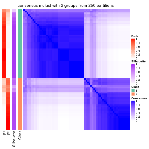
consensus_heatmap(res, k = 3)
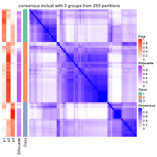
consensus_heatmap(res, k = 4)

consensus_heatmap(res, k = 5)
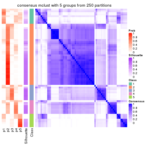
consensus_heatmap(res, k = 6)
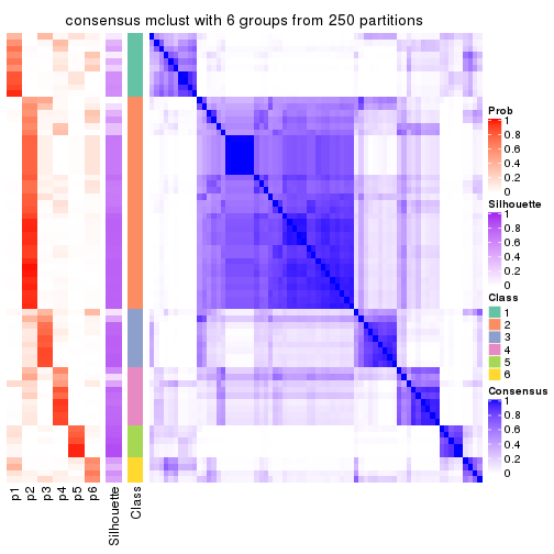
Heatmaps for the membership of samples in all partitions to see how consistent they are:
membership_heatmap(res, k = 2)
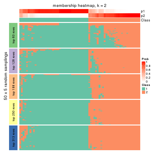
membership_heatmap(res, k = 3)
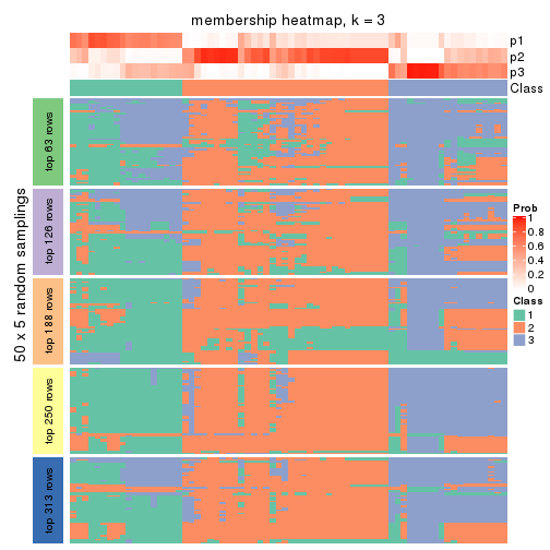
membership_heatmap(res, k = 4)
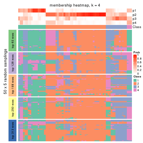
membership_heatmap(res, k = 5)
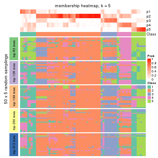
membership_heatmap(res, k = 6)
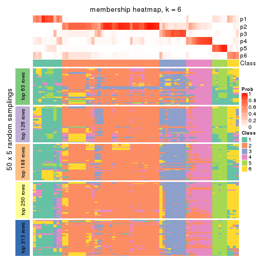
As soon as we have had the classes for columns, we can look for signatures which are significantly different between classes which can be candidate marks for certain classes. Following are the heatmaps for signatures.
Signature heatmaps where rows are scaled:
get_signatures(res, k = 2)
get_signatures(res, k = 3)
get_signatures(res, k = 4)
get_signatures(res, k = 5)
get_signatures(res, k = 6)
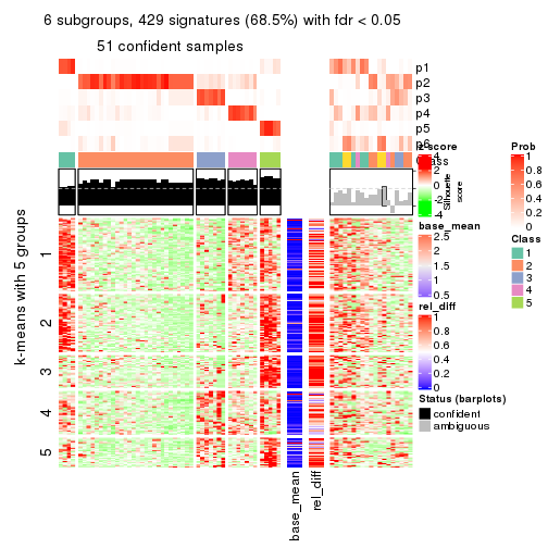
Signature heatmaps where rows are not scaled:
get_signatures(res, k = 2, scale_rows = FALSE)
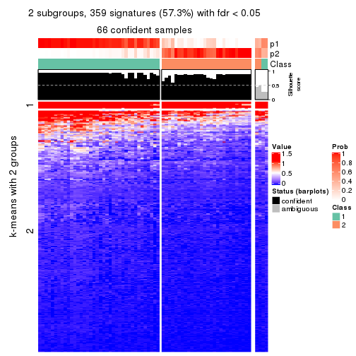
get_signatures(res, k = 3, scale_rows = FALSE)
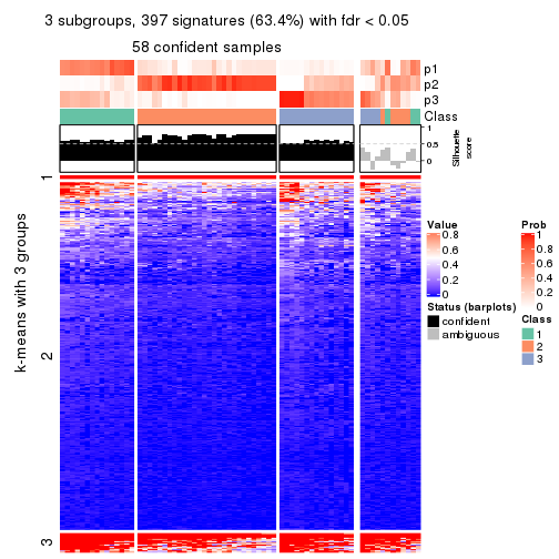
get_signatures(res, k = 4, scale_rows = FALSE)
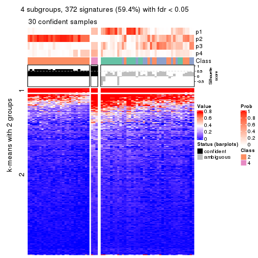
get_signatures(res, k = 5, scale_rows = FALSE)
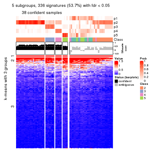
get_signatures(res, k = 6, scale_rows = FALSE)
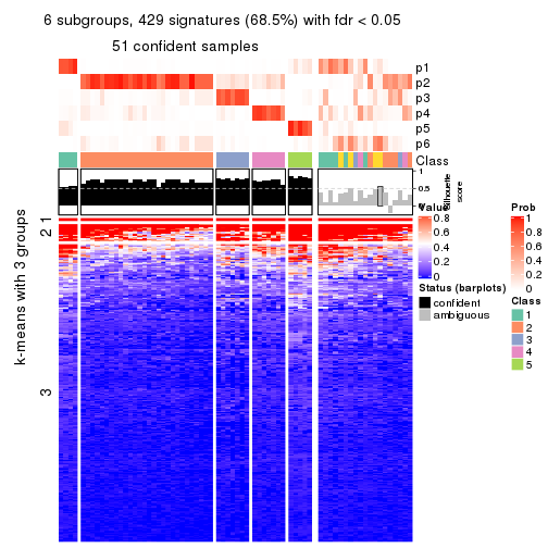
Compare the overlap of signatures from different k:
compare_signatures(res)
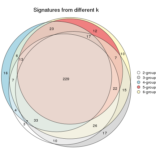
get_signature() returns a data frame invisibly. TO get the list of signatures, the function
call should be assigned to a variable explicitly. In following code, if plot argument is set
to FALSE, no heatmap is plotted while only the differential analysis is performed.
# code only for demonstration
tb = get_signature(res, k = ..., plot = FALSE)
An example of the output of tb is:
#> which_row fdr mean_1 mean_2 scaled_mean_1 scaled_mean_2 km
#> 1 38 0.042760348 8.373488 9.131774 -0.5533452 0.5164555 1
#> 2 40 0.018707592 7.106213 8.469186 -0.6173731 0.5762149 1
#> 3 55 0.019134737 10.221463 11.207825 -0.6159697 0.5749050 1
#> 4 59 0.006059896 5.921854 7.869574 -0.6899429 0.6439467 1
#> 5 60 0.018055526 8.928898 10.211722 -0.6204761 0.5791110 1
#> 6 98 0.009384629 15.714769 14.887706 0.6635654 -0.6193277 2
...
The columns in tb are:
which_row: row indices corresponding to the input matrix.fdr: FDR for the differential test. mean_x: The mean value in group x.scaled_mean_x: The mean value in group x after rows are scaled.km: Row groups if k-means clustering is applied to rows.UMAP plot which shows how samples are separated.
dimension_reduction(res, k = 2, method = "UMAP")
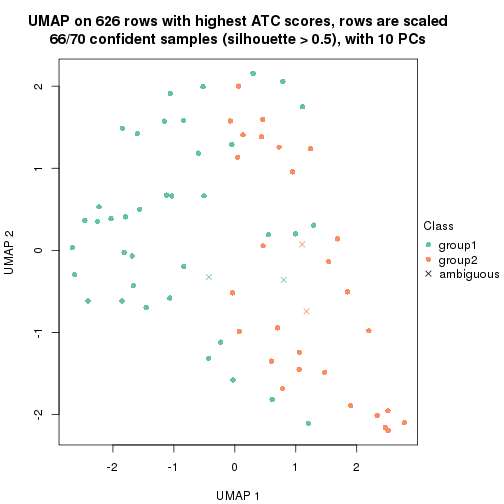
dimension_reduction(res, k = 3, method = "UMAP")
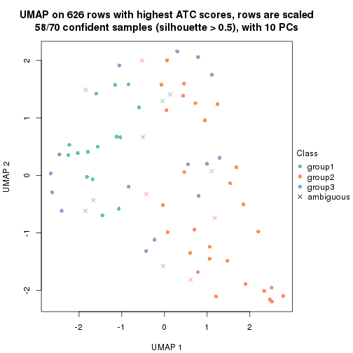
dimension_reduction(res, k = 4, method = "UMAP")
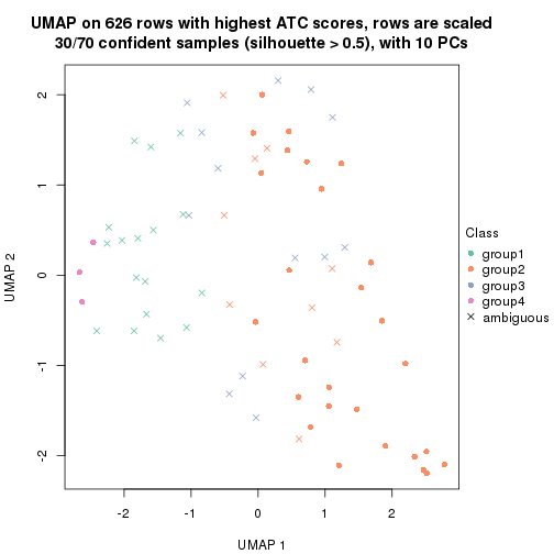
dimension_reduction(res, k = 5, method = "UMAP")
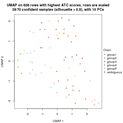
dimension_reduction(res, k = 6, method = "UMAP")
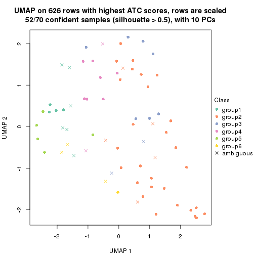
Following heatmap shows how subgroups are split when increasing k:
collect_classes(res)
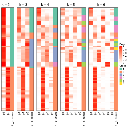
If matrix rows can be associated to genes, consider to use functional_enrichment(res,
...) to perform function enrichment for the signature genes. See this vignette for more detailed explanations.
The object with results only for a single top-value method and a single partition method can be extracted as:
res = res_list["ATC", "NMF"]
# you can also extract it by
# res = res_list["ATC:NMF"]
A summary of res and all the functions that can be applied to it:
res
#> A 'ConsensusPartition' object with k = 2, 3, 4, 5, 6.
#> On a matrix with 626 rows and 70 columns.
#> Top rows (63, 126, 188, 250, 313) are extracted by 'ATC' method.
#> Subgroups are detected by 'NMF' method.
#> Performed in total 1250 partitions by row resampling.
#> Best k for subgroups seems to be 3.
#>
#> Following methods can be applied to this 'ConsensusPartition' object:
#> [1] "cola_report" "collect_classes" "collect_plots"
#> [4] "collect_stats" "colnames" "compare_signatures"
#> [7] "consensus_heatmap" "dimension_reduction" "functional_enrichment"
#> [10] "get_anno_col" "get_anno" "get_classes"
#> [13] "get_consensus" "get_matrix" "get_membership"
#> [16] "get_param" "get_signatures" "get_stats"
#> [19] "is_best_k" "is_stable_k" "membership_heatmap"
#> [22] "ncol" "nrow" "plot_ecdf"
#> [25] "rownames" "select_partition_number" "show"
#> [28] "suggest_best_k" "test_to_known_factors"
collect_plots() function collects all the plots made from res for all k (number of partitions)
into one single page to provide an easy and fast comparison between different k.
collect_plots(res)
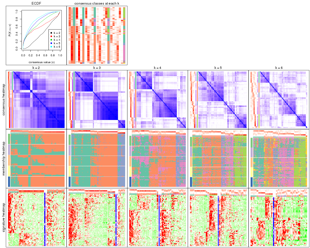
The plots are:
k and the heatmap of
predicted classes for each k.k.k.k.All the plots in panels can be made by individual functions and they are plotted later in this section.
select_partition_number() produces several plots showing different
statistics for choosing “optimized” k. There are following statistics:
k;k, the area increased is defined as \(A_k - A_{k-1}\).The detailed explanations of these statistics can be found in the cola vignette.
Generally speaking, lower PAC score, higher mean silhouette score or higher
concordance corresponds to better partition. Rand index and Jaccard index
measure how similar the current partition is compared to partition with k-1.
If they are too similar, we won't accept k is better than k-1.
select_partition_number(res)
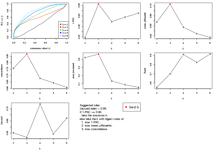
The numeric values for all these statistics can be obtained by get_stats().
get_stats(res)
#> k 1-PAC mean_silhouette concordance area_increased Rand Jaccard
#> 2 2 0.196 0.538 0.756 0.4200 0.552 0.552
#> 3 3 0.512 0.716 0.866 0.4613 0.699 0.516
#> 4 4 0.346 0.487 0.678 0.1346 0.911 0.786
#> 5 5 0.388 0.422 0.643 0.0892 0.825 0.544
#> 6 6 0.426 0.386 0.608 0.0576 0.914 0.672
suggest_best_k() suggests the best \(k\) based on these statistics. The rules are as follows:
suggest_best_k(res)
#> [1] 3
Following shows the table of the partitions (You need to click the show/hide
code output link to see it). The membership matrix (columns with name p*)
is inferred by
clue::cl_consensus()
function with the SE method. Basically the value in the membership matrix
represents the probability to belong to a certain group. The finall class
label for an item is determined with the group with highest probability it
belongs to.
In get_classes() function, the entropy is calculated from the membership
matrix and the silhouette score is calculated from the consensus matrix.
cbind(get_classes(res, k = 2), get_membership(res, k = 2))
#> class entropy silhouette p1 p2
#> SRR837437 2 0.8144 0.4958 0.252 0.748
#> SRR837438 2 0.2603 0.7285 0.044 0.956
#> SRR837439 2 0.0000 0.7401 0.000 1.000
#> SRR837440 2 0.1414 0.7347 0.020 0.980
#> SRR837441 2 0.0000 0.7401 0.000 1.000
#> SRR837442 2 0.9815 0.0502 0.420 0.580
#> SRR837443 2 0.0938 0.7369 0.012 0.988
#> SRR837444 2 0.0000 0.7401 0.000 1.000
#> SRR837445 2 0.7602 0.5895 0.220 0.780
#> SRR837446 2 0.3879 0.6863 0.076 0.924
#> SRR837447 2 0.6148 0.6554 0.152 0.848
#> SRR837448 1 0.9087 0.5849 0.676 0.324
#> SRR837449 2 0.7376 0.6062 0.208 0.792
#> SRR837450 1 0.7950 0.6076 0.760 0.240
#> SRR837451 2 0.0376 0.7402 0.004 0.996
#> SRR837452 2 0.4298 0.7058 0.088 0.912
#> SRR837453 2 0.2778 0.7328 0.048 0.952
#> SRR837454 2 0.1843 0.7358 0.028 0.972
#> SRR837455 2 0.8443 0.5094 0.272 0.728
#> SRR837456 2 0.9754 0.1284 0.408 0.592
#> SRR837457 2 0.2043 0.7272 0.032 0.968
#> SRR837458 1 0.9922 0.4061 0.552 0.448
#> SRR837459 2 0.1633 0.7317 0.024 0.976
#> SRR837460 2 0.3114 0.7074 0.056 0.944
#> SRR837461 2 0.2778 0.7152 0.048 0.952
#> SRR837462 2 0.0672 0.7382 0.008 0.992
#> SRR837463 2 0.0000 0.7401 0.000 1.000
#> SRR837464 2 0.3114 0.7078 0.056 0.944
#> SRR837465 2 0.0000 0.7401 0.000 1.000
#> SRR837466 1 0.9087 0.5849 0.676 0.324
#> SRR837467 2 0.2948 0.7170 0.052 0.948
#> SRR837468 2 0.9580 0.2007 0.380 0.620
#> SRR837469 2 0.0376 0.7393 0.004 0.996
#> SRR837470 2 0.2778 0.7363 0.048 0.952
#> SRR837471 1 0.9866 0.4478 0.568 0.432
#> SRR837472 1 0.9686 0.5122 0.604 0.396
#> SRR837473 1 0.9833 0.4672 0.576 0.424
#> SRR837474 2 0.9909 -0.0387 0.444 0.556
#> SRR837475 1 0.9661 0.5191 0.608 0.392
#> SRR837476 2 0.8144 0.5390 0.252 0.748
#> SRR837477 1 0.8499 0.6029 0.724 0.276
#> SRR837478 1 0.4161 0.5750 0.916 0.084
#> SRR837479 1 0.7299 0.4672 0.796 0.204
#> SRR837480 1 0.6247 0.5203 0.844 0.156
#> SRR837481 1 0.8267 0.5467 0.740 0.260
#> SRR837482 1 0.9944 0.0853 0.544 0.456
#> SRR837483 1 0.7139 0.6077 0.804 0.196
#> SRR837484 1 0.6247 0.5405 0.844 0.156
#> SRR837485 1 0.7815 0.5482 0.768 0.232
#> SRR837486 1 0.5059 0.5287 0.888 0.112
#> SRR837487 2 0.9944 -0.2394 0.456 0.544
#> SRR837488 1 0.9909 0.4209 0.556 0.444
#> SRR837489 2 0.9323 0.3308 0.348 0.652
#> SRR837490 2 0.8081 0.5509 0.248 0.752
#> SRR837491 2 0.8661 0.4817 0.288 0.712
#> SRR837492 1 0.9323 0.5653 0.652 0.348
#> SRR837493 2 0.0672 0.7402 0.008 0.992
#> SRR837494 2 0.2043 0.7280 0.032 0.968
#> SRR837495 2 0.9209 0.3701 0.336 0.664
#> SRR837496 1 0.9795 0.4815 0.584 0.416
#> SRR837497 2 0.8661 0.4797 0.288 0.712
#> SRR837498 2 0.1843 0.7359 0.028 0.972
#> SRR837499 2 0.8608 0.4900 0.284 0.716
#> SRR837500 2 0.9635 0.2039 0.388 0.612
#> SRR837501 2 0.9710 0.1614 0.400 0.600
#> SRR837502 2 0.6712 0.6345 0.176 0.824
#> SRR837503 1 0.9954 0.3735 0.540 0.460
#> SRR837504 2 0.2043 0.7271 0.032 0.968
#> SRR837505 2 0.9944 0.0547 0.456 0.544
#> SRR837506 1 0.7453 0.4579 0.788 0.212
cbind(get_classes(res, k = 3), get_membership(res, k = 3))
#> class entropy silhouette p1 p2 p3
#> SRR837437 2 0.6998 0.5322 0.292 0.664 0.044
#> SRR837438 2 0.1711 0.8551 0.032 0.960 0.008
#> SRR837439 2 0.0000 0.8598 0.000 1.000 0.000
#> SRR837440 2 0.1753 0.8457 0.000 0.952 0.048
#> SRR837441 2 0.0000 0.8598 0.000 1.000 0.000
#> SRR837442 1 0.3933 0.7773 0.880 0.092 0.028
#> SRR837443 2 0.0592 0.8573 0.000 0.988 0.012
#> SRR837444 2 0.0000 0.8598 0.000 1.000 0.000
#> SRR837445 1 0.6291 0.1424 0.532 0.468 0.000
#> SRR837446 2 0.3038 0.7988 0.000 0.896 0.104
#> SRR837447 2 0.4702 0.7060 0.212 0.788 0.000
#> SRR837448 1 0.1289 0.7867 0.968 0.000 0.032
#> SRR837449 2 0.5843 0.6494 0.252 0.732 0.016
#> SRR837450 1 0.1765 0.7857 0.956 0.004 0.040
#> SRR837451 2 0.0592 0.8590 0.012 0.988 0.000
#> SRR837452 2 0.3816 0.7756 0.148 0.852 0.000
#> SRR837453 2 0.2793 0.8458 0.028 0.928 0.044
#> SRR837454 2 0.1411 0.8525 0.036 0.964 0.000
#> SRR837455 2 0.6140 0.3495 0.404 0.596 0.000
#> SRR837456 1 0.5178 0.6335 0.744 0.256 0.000
#> SRR837457 2 0.0475 0.8602 0.004 0.992 0.004
#> SRR837458 1 0.1170 0.7957 0.976 0.008 0.016
#> SRR837459 2 0.0592 0.8592 0.000 0.988 0.012
#> SRR837460 2 0.1267 0.8564 0.004 0.972 0.024
#> SRR837461 2 0.0747 0.8563 0.000 0.984 0.016
#> SRR837462 2 0.0661 0.8598 0.004 0.988 0.008
#> SRR837463 2 0.0237 0.8594 0.000 0.996 0.004
#> SRR837464 2 0.1289 0.8517 0.000 0.968 0.032
#> SRR837465 2 0.0237 0.8599 0.004 0.996 0.000
#> SRR837466 1 0.1753 0.7787 0.952 0.000 0.048
#> SRR837467 2 0.3644 0.7920 0.004 0.872 0.124
#> SRR837468 2 0.6309 -0.0399 0.000 0.504 0.496
#> SRR837469 2 0.0237 0.8594 0.000 0.996 0.004
#> SRR837470 2 0.5243 0.7781 0.072 0.828 0.100
#> SRR837471 1 0.0592 0.7957 0.988 0.012 0.000
#> SRR837472 1 0.1267 0.7927 0.972 0.004 0.024
#> SRR837473 1 0.1163 0.7971 0.972 0.028 0.000
#> SRR837474 1 0.1529 0.7950 0.960 0.040 0.000
#> SRR837475 1 0.0000 0.7943 1.000 0.000 0.000
#> SRR837476 2 0.6252 0.1928 0.444 0.556 0.000
#> SRR837477 1 0.3686 0.7148 0.860 0.000 0.140
#> SRR837478 1 0.5650 0.4245 0.688 0.000 0.312
#> SRR837479 3 0.0237 0.8388 0.004 0.000 0.996
#> SRR837480 3 0.3941 0.7819 0.156 0.000 0.844
#> SRR837481 3 0.4605 0.7502 0.204 0.000 0.796
#> SRR837482 3 0.2261 0.8271 0.000 0.068 0.932
#> SRR837483 1 0.4842 0.6176 0.776 0.000 0.224
#> SRR837484 3 0.3983 0.8006 0.144 0.004 0.852
#> SRR837485 3 0.6890 0.5063 0.340 0.028 0.632
#> SRR837486 3 0.1964 0.8384 0.056 0.000 0.944
#> SRR837487 1 0.8726 0.3986 0.564 0.140 0.296
#> SRR837488 1 0.5304 0.7420 0.824 0.108 0.068
#> SRR837489 1 0.5058 0.6674 0.756 0.244 0.000
#> SRR837490 2 0.6111 0.3540 0.396 0.604 0.000
#> SRR837491 2 0.6912 0.2003 0.444 0.540 0.016
#> SRR837492 1 0.1163 0.7885 0.972 0.000 0.028
#> SRR837493 2 0.0424 0.8599 0.008 0.992 0.000
#> SRR837494 2 0.1289 0.8529 0.000 0.968 0.032
#> SRR837495 1 0.4062 0.7332 0.836 0.164 0.000
#> SRR837496 1 0.0237 0.7952 0.996 0.004 0.000
#> SRR837497 1 0.4887 0.6809 0.772 0.228 0.000
#> SRR837498 2 0.1753 0.8467 0.048 0.952 0.000
#> SRR837499 1 0.6192 0.2617 0.580 0.420 0.000
#> SRR837500 1 0.5497 0.5655 0.708 0.292 0.000
#> SRR837501 3 0.4842 0.6817 0.000 0.224 0.776
#> SRR837502 2 0.5216 0.6496 0.260 0.740 0.000
#> SRR837503 1 0.0592 0.7957 0.988 0.012 0.000
#> SRR837504 2 0.0424 0.8582 0.000 0.992 0.008
#> SRR837505 3 0.2356 0.8246 0.000 0.072 0.928
#> SRR837506 3 0.0592 0.8392 0.012 0.000 0.988
cbind(get_classes(res, k = 4), get_membership(res, k = 4))
#> class entropy silhouette p1 p2 p3 p4
#> SRR837437 2 0.8186 0.1510 0.132 0.428 0.044 0.396
#> SRR837438 2 0.4994 0.7015 0.044 0.796 0.032 0.128
#> SRR837439 2 0.2039 0.7328 0.016 0.940 0.008 0.036
#> SRR837440 2 0.3770 0.7067 0.004 0.852 0.040 0.104
#> SRR837441 2 0.2384 0.7265 0.016 0.928 0.040 0.016
#> SRR837442 1 0.6158 0.2172 0.592 0.052 0.004 0.352
#> SRR837443 2 0.3134 0.7114 0.004 0.884 0.024 0.088
#> SRR837444 2 0.1510 0.7296 0.016 0.956 0.028 0.000
#> SRR837445 2 0.7638 0.0414 0.412 0.456 0.028 0.104
#> SRR837446 2 0.6208 0.5598 0.004 0.684 0.168 0.144
#> SRR837447 2 0.6948 0.4788 0.204 0.588 0.208 0.000
#> SRR837448 1 0.4907 0.4990 0.764 0.000 0.060 0.176
#> SRR837449 2 0.7732 0.5256 0.172 0.588 0.196 0.044
#> SRR837450 1 0.5012 0.5432 0.772 0.000 0.112 0.116
#> SRR837451 2 0.2983 0.7242 0.008 0.880 0.108 0.004
#> SRR837452 2 0.6277 0.6231 0.116 0.680 0.196 0.008
#> SRR837453 2 0.5872 0.6619 0.032 0.704 0.228 0.036
#> SRR837454 2 0.3787 0.7062 0.036 0.840 0.124 0.000
#> SRR837455 2 0.7615 0.3874 0.280 0.544 0.156 0.020
#> SRR837456 1 0.6811 0.4477 0.612 0.240 0.144 0.004
#> SRR837457 2 0.2302 0.7286 0.008 0.924 0.060 0.008
#> SRR837458 1 0.4901 0.4995 0.764 0.004 0.044 0.188
#> SRR837459 2 0.2777 0.7273 0.004 0.888 0.104 0.004
#> SRR837460 2 0.6517 0.5911 0.004 0.648 0.136 0.212
#> SRR837461 2 0.5031 0.6462 0.000 0.768 0.092 0.140
#> SRR837462 2 0.1635 0.7323 0.008 0.948 0.044 0.000
#> SRR837463 2 0.3771 0.7131 0.004 0.856 0.052 0.088
#> SRR837464 2 0.5330 0.6451 0.000 0.748 0.132 0.120
#> SRR837465 2 0.2319 0.7332 0.016 0.932 0.028 0.024
#> SRR837466 1 0.4508 0.5020 0.780 0.000 0.036 0.184
#> SRR837467 2 0.7669 0.2900 0.008 0.472 0.172 0.348
#> SRR837468 2 0.7803 -0.1821 0.000 0.404 0.340 0.256
#> SRR837469 2 0.2376 0.7287 0.016 0.916 0.068 0.000
#> SRR837470 2 0.6730 0.5699 0.076 0.672 0.048 0.204
#> SRR837471 1 0.1109 0.5905 0.968 0.004 0.000 0.028
#> SRR837472 1 0.3082 0.5671 0.884 0.000 0.032 0.084
#> SRR837473 1 0.2708 0.5876 0.904 0.016 0.004 0.076
#> SRR837474 1 0.4637 0.5575 0.816 0.116 0.024 0.044
#> SRR837475 1 0.1474 0.5856 0.948 0.000 0.000 0.052
#> SRR837476 1 0.7459 0.0663 0.476 0.404 0.096 0.024
#> SRR837477 1 0.5599 0.3396 0.672 0.000 0.052 0.276
#> SRR837478 4 0.5805 0.3536 0.388 0.000 0.036 0.576
#> SRR837479 4 0.4188 -0.0450 0.004 0.000 0.244 0.752
#> SRR837480 4 0.6471 0.3434 0.144 0.004 0.196 0.656
#> SRR837481 3 0.6380 0.0763 0.052 0.004 0.476 0.468
#> SRR837482 3 0.6504 0.5045 0.000 0.072 0.476 0.452
#> SRR837483 1 0.6419 -0.0753 0.512 0.000 0.068 0.420
#> SRR837484 4 0.3082 0.4130 0.040 0.008 0.056 0.896
#> SRR837485 4 0.6669 0.3566 0.132 0.016 0.192 0.660
#> SRR837486 4 0.3542 0.4630 0.076 0.000 0.060 0.864
#> SRR837487 4 0.7531 0.4618 0.208 0.052 0.128 0.612
#> SRR837488 4 0.7589 0.4099 0.304 0.064 0.072 0.560
#> SRR837489 1 0.8966 0.2380 0.440 0.276 0.204 0.080
#> SRR837490 2 0.8874 0.3308 0.264 0.464 0.188 0.084
#> SRR837491 2 0.9498 0.2866 0.248 0.408 0.164 0.180
#> SRR837492 1 0.5144 0.4588 0.732 0.000 0.052 0.216
#> SRR837493 2 0.2555 0.7347 0.032 0.920 0.040 0.008
#> SRR837494 2 0.5055 0.6555 0.004 0.768 0.068 0.160
#> SRR837495 1 0.6097 0.5206 0.724 0.160 0.084 0.032
#> SRR837496 1 0.4044 0.5855 0.852 0.032 0.088 0.028
#> SRR837497 1 0.7521 0.3327 0.528 0.316 0.140 0.016
#> SRR837498 2 0.4764 0.6831 0.088 0.788 0.124 0.000
#> SRR837499 1 0.7579 0.1517 0.496 0.376 0.096 0.032
#> SRR837500 1 0.7159 0.4430 0.620 0.228 0.124 0.028
#> SRR837501 3 0.7140 0.4723 0.000 0.204 0.560 0.236
#> SRR837502 2 0.7691 0.4812 0.224 0.560 0.192 0.024
#> SRR837503 1 0.2616 0.5925 0.920 0.016 0.036 0.028
#> SRR837504 2 0.0895 0.7275 0.000 0.976 0.020 0.004
#> SRR837505 3 0.6678 0.5446 0.000 0.088 0.500 0.412
#> SRR837506 3 0.4936 0.4777 0.004 0.000 0.624 0.372
cbind(get_classes(res, k = 5), get_membership(res, k = 5))
#> class entropy silhouette p1 p2 p3 p4 p5
#> SRR837437 4 0.609 0.1730 0.040 0.348 0.012 0.568 0.032
#> SRR837438 2 0.514 0.5624 0.060 0.748 0.024 0.152 0.016
#> SRR837439 2 0.249 0.6041 0.068 0.904 0.008 0.016 0.004
#> SRR837440 2 0.456 0.6143 0.028 0.784 0.080 0.108 0.000
#> SRR837441 2 0.259 0.6187 0.068 0.900 0.020 0.008 0.004
#> SRR837442 5 0.749 0.0548 0.068 0.108 0.012 0.376 0.436
#> SRR837443 2 0.230 0.6310 0.032 0.912 0.004 0.052 0.000
#> SRR837444 2 0.173 0.6170 0.044 0.940 0.004 0.008 0.004
#> SRR837445 2 0.793 -0.1126 0.140 0.412 0.008 0.100 0.340
#> SRR837446 2 0.689 0.4306 0.088 0.612 0.192 0.096 0.012
#> SRR837447 1 0.513 0.4916 0.568 0.388 0.000 0.000 0.044
#> SRR837448 5 0.516 0.5606 0.148 0.000 0.004 0.144 0.704
#> SRR837449 1 0.644 0.5530 0.572 0.316 0.016 0.032 0.064
#> SRR837450 5 0.503 0.5647 0.212 0.000 0.012 0.068 0.708
#> SRR837451 2 0.530 0.1763 0.348 0.604 0.036 0.008 0.004
#> SRR837452 1 0.542 0.5188 0.608 0.336 0.004 0.012 0.040
#> SRR837453 1 0.589 0.3626 0.544 0.380 0.016 0.056 0.004
#> SRR837454 2 0.440 -0.1507 0.432 0.564 0.004 0.000 0.000
#> SRR837455 1 0.634 0.5952 0.556 0.304 0.000 0.020 0.120
#> SRR837456 1 0.650 0.2455 0.444 0.120 0.000 0.016 0.420
#> SRR837457 2 0.455 0.6022 0.120 0.772 0.096 0.012 0.000
#> SRR837458 5 0.569 0.5208 0.092 0.016 0.008 0.208 0.676
#> SRR837459 2 0.538 0.5352 0.152 0.712 0.116 0.016 0.004
#> SRR837460 2 0.818 0.2965 0.164 0.456 0.104 0.256 0.020
#> SRR837461 2 0.643 0.5257 0.088 0.644 0.120 0.148 0.000
#> SRR837462 2 0.307 0.6008 0.112 0.860 0.016 0.012 0.000
#> SRR837463 2 0.490 0.6031 0.076 0.764 0.044 0.116 0.000
#> SRR837464 2 0.704 0.4621 0.128 0.584 0.160 0.128 0.000
#> SRR837465 2 0.361 0.6119 0.128 0.832 0.024 0.012 0.004
#> SRR837466 5 0.473 0.5276 0.076 0.000 0.000 0.208 0.716
#> SRR837467 2 0.803 0.0124 0.112 0.376 0.188 0.324 0.000
#> SRR837468 3 0.733 0.3317 0.044 0.320 0.444 0.192 0.000
#> SRR837469 2 0.379 0.4842 0.204 0.776 0.016 0.000 0.004
#> SRR837470 2 0.754 0.4042 0.084 0.576 0.092 0.200 0.048
#> SRR837471 5 0.199 0.6349 0.048 0.008 0.000 0.016 0.928
#> SRR837472 5 0.323 0.6301 0.084 0.000 0.000 0.064 0.852
#> SRR837473 5 0.258 0.6336 0.024 0.024 0.000 0.048 0.904
#> SRR837474 5 0.494 0.5243 0.076 0.140 0.000 0.032 0.752
#> SRR837475 5 0.122 0.6348 0.020 0.000 0.000 0.020 0.960
#> SRR837476 5 0.665 -0.1354 0.200 0.300 0.000 0.008 0.492
#> SRR837477 5 0.579 0.3727 0.048 0.000 0.044 0.280 0.628
#> SRR837478 4 0.607 0.4119 0.080 0.004 0.024 0.604 0.288
#> SRR837479 4 0.585 0.2092 0.084 0.012 0.264 0.632 0.008
#> SRR837480 4 0.679 0.3722 0.060 0.008 0.220 0.600 0.112
#> SRR837481 4 0.768 0.2103 0.268 0.008 0.232 0.444 0.048
#> SRR837482 3 0.654 0.3810 0.084 0.048 0.540 0.328 0.000
#> SRR837483 4 0.530 -0.1070 0.032 0.000 0.008 0.480 0.480
#> SRR837484 4 0.410 0.4894 0.032 0.004 0.088 0.824 0.052
#> SRR837485 4 0.688 0.4517 0.204 0.020 0.060 0.612 0.104
#> SRR837486 4 0.272 0.5063 0.000 0.000 0.048 0.884 0.068
#> SRR837487 4 0.717 0.4695 0.128 0.064 0.072 0.632 0.104
#> SRR837488 4 0.656 0.5239 0.136 0.052 0.016 0.648 0.148
#> SRR837489 1 0.719 0.5416 0.556 0.156 0.008 0.060 0.220
#> SRR837490 1 0.694 0.5849 0.588 0.220 0.008 0.068 0.116
#> SRR837491 1 0.816 0.4815 0.464 0.240 0.016 0.160 0.120
#> SRR837492 5 0.515 0.4572 0.068 0.000 0.004 0.264 0.664
#> SRR837493 2 0.430 0.5830 0.156 0.788 0.032 0.016 0.008
#> SRR837494 2 0.565 0.5742 0.068 0.696 0.060 0.176 0.000
#> SRR837495 5 0.730 0.2694 0.184 0.184 0.028 0.040 0.564
#> SRR837496 5 0.489 0.5646 0.196 0.020 0.016 0.028 0.740
#> SRR837497 1 0.756 0.2452 0.360 0.276 0.024 0.008 0.332
#> SRR837498 2 0.554 0.2096 0.316 0.616 0.040 0.000 0.028
#> SRR837499 5 0.744 -0.3863 0.244 0.324 0.004 0.028 0.400
#> SRR837500 1 0.720 0.4105 0.452 0.152 0.000 0.048 0.348
#> SRR837501 3 0.579 0.5568 0.056 0.124 0.696 0.124 0.000
#> SRR837502 1 0.691 0.5314 0.508 0.328 0.008 0.028 0.128
#> SRR837503 5 0.221 0.6326 0.060 0.012 0.000 0.012 0.916
#> SRR837504 2 0.283 0.6067 0.072 0.888 0.028 0.008 0.004
#> SRR837505 3 0.619 0.5252 0.044 0.104 0.632 0.220 0.000
#> SRR837506 3 0.525 0.3105 0.104 0.000 0.704 0.180 0.012
cbind(get_classes(res, k = 6), get_membership(res, k = 6))
#> class entropy silhouette p1 p2 p3 p4 p5 p6
#> SRR837437 2 0.593 0.2431 0.032 0.608 0.088 0.252 0.016 0.004
#> SRR837438 4 0.513 0.5083 0.068 0.120 0.072 0.728 0.008 0.004
#> SRR837439 4 0.218 0.5807 0.048 0.008 0.028 0.912 0.004 0.000
#> SRR837440 4 0.358 0.5273 0.012 0.052 0.128 0.808 0.000 0.000
#> SRR837441 4 0.274 0.5759 0.060 0.004 0.056 0.876 0.004 0.000
#> SRR837442 2 0.752 0.1211 0.044 0.380 0.084 0.132 0.360 0.000
#> SRR837443 4 0.297 0.5464 0.008 0.028 0.096 0.860 0.000 0.008
#> SRR837444 4 0.290 0.5784 0.056 0.016 0.044 0.876 0.008 0.000
#> SRR837445 4 0.870 -0.0126 0.128 0.116 0.184 0.316 0.252 0.004
#> SRR837446 4 0.653 0.2739 0.040 0.084 0.240 0.584 0.008 0.044
#> SRR837447 1 0.431 0.5895 0.736 0.008 0.020 0.212 0.020 0.004
#> SRR837448 5 0.557 0.5581 0.148 0.148 0.036 0.000 0.660 0.008
#> SRR837449 1 0.541 0.6036 0.696 0.064 0.044 0.172 0.020 0.004
#> SRR837450 5 0.562 0.5375 0.240 0.060 0.024 0.000 0.640 0.036
#> SRR837451 1 0.578 0.0538 0.448 0.000 0.152 0.396 0.000 0.004
#> SRR837452 1 0.522 0.6147 0.712 0.020 0.084 0.156 0.020 0.008
#> SRR837453 1 0.604 0.4827 0.612 0.072 0.096 0.212 0.000 0.008
#> SRR837454 1 0.483 0.4284 0.596 0.004 0.040 0.352 0.008 0.000
#> SRR837455 1 0.518 0.6229 0.724 0.052 0.036 0.140 0.048 0.000
#> SRR837456 1 0.530 0.4623 0.660 0.024 0.012 0.060 0.240 0.004
#> SRR837457 4 0.565 0.3823 0.172 0.004 0.228 0.588 0.000 0.008
#> SRR837458 5 0.573 0.4854 0.112 0.236 0.044 0.000 0.608 0.000
#> SRR837459 4 0.570 0.4305 0.132 0.004 0.220 0.616 0.000 0.028
#> SRR837460 3 0.747 0.3284 0.140 0.228 0.344 0.288 0.000 0.000
#> SRR837461 4 0.635 -0.1740 0.056 0.088 0.384 0.464 0.000 0.008
#> SRR837462 4 0.379 0.5674 0.116 0.008 0.072 0.800 0.000 0.004
#> SRR837463 4 0.623 0.2678 0.124 0.080 0.224 0.572 0.000 0.000
#> SRR837464 3 0.614 0.2158 0.088 0.040 0.484 0.380 0.000 0.008
#> SRR837465 4 0.454 0.4495 0.100 0.008 0.176 0.716 0.000 0.000
#> SRR837466 5 0.529 0.5109 0.072 0.252 0.024 0.000 0.644 0.008
#> SRR837467 3 0.724 0.3860 0.052 0.220 0.424 0.284 0.004 0.016
#> SRR837468 3 0.719 0.3191 0.024 0.076 0.476 0.252 0.000 0.172
#> SRR837469 4 0.464 0.4093 0.248 0.004 0.076 0.672 0.000 0.000
#> SRR837470 4 0.846 0.1282 0.136 0.144 0.200 0.428 0.056 0.036
#> SRR837471 5 0.151 0.6378 0.036 0.004 0.012 0.000 0.944 0.004
#> SRR837472 5 0.281 0.6371 0.048 0.052 0.012 0.000 0.880 0.008
#> SRR837473 5 0.249 0.6379 0.028 0.032 0.016 0.020 0.904 0.000
#> SRR837474 5 0.398 0.5734 0.048 0.016 0.008 0.140 0.788 0.000
#> SRR837475 5 0.148 0.6417 0.020 0.032 0.004 0.000 0.944 0.000
#> SRR837476 5 0.712 0.0298 0.184 0.024 0.052 0.296 0.444 0.000
#> SRR837477 5 0.615 0.3833 0.040 0.300 0.036 0.000 0.564 0.060
#> SRR837478 2 0.627 0.4187 0.056 0.628 0.072 0.000 0.184 0.060
#> SRR837479 2 0.633 0.2460 0.016 0.524 0.132 0.000 0.028 0.300
#> SRR837480 2 0.642 0.2886 0.012 0.504 0.336 0.000 0.080 0.068
#> SRR837481 2 0.762 0.1972 0.240 0.400 0.080 0.008 0.016 0.256
#> SRR837482 3 0.691 -0.0447 0.036 0.184 0.528 0.036 0.004 0.212
#> SRR837483 2 0.513 0.0420 0.008 0.524 0.028 0.000 0.420 0.020
#> SRR837484 2 0.441 0.4828 0.012 0.776 0.056 0.000 0.040 0.116
#> SRR837485 2 0.715 0.4021 0.156 0.580 0.092 0.020 0.044 0.108
#> SRR837486 2 0.347 0.5013 0.008 0.848 0.064 0.004 0.048 0.028
#> SRR837487 2 0.709 0.4336 0.068 0.596 0.148 0.024 0.100 0.064
#> SRR837488 2 0.535 0.5219 0.088 0.716 0.048 0.032 0.116 0.000
#> SRR837489 1 0.665 0.5298 0.600 0.056 0.120 0.160 0.064 0.000
#> SRR837490 1 0.580 0.5715 0.680 0.044 0.104 0.136 0.032 0.004
#> SRR837491 1 0.692 0.4623 0.564 0.168 0.140 0.088 0.040 0.000
#> SRR837492 5 0.576 0.3617 0.076 0.344 0.028 0.000 0.544 0.008
#> SRR837493 4 0.561 0.5260 0.156 0.024 0.132 0.668 0.016 0.004
#> SRR837494 4 0.622 0.3554 0.084 0.096 0.204 0.604 0.000 0.012
#> SRR837495 5 0.801 0.2551 0.188 0.068 0.112 0.164 0.460 0.008
#> SRR837496 5 0.660 0.5259 0.160 0.052 0.116 0.028 0.620 0.024
#> SRR837497 1 0.823 0.1445 0.324 0.048 0.120 0.296 0.208 0.004
#> SRR837498 4 0.592 0.2600 0.276 0.016 0.120 0.572 0.016 0.000
#> SRR837499 4 0.757 -0.2559 0.304 0.064 0.028 0.340 0.264 0.000
#> SRR837500 1 0.634 0.5120 0.604 0.076 0.040 0.064 0.216 0.000
#> SRR837501 3 0.619 -0.2723 0.024 0.064 0.552 0.052 0.000 0.308
#> SRR837502 1 0.663 0.5255 0.548 0.012 0.164 0.208 0.068 0.000
#> SRR837503 5 0.403 0.6165 0.072 0.036 0.040 0.028 0.820 0.004
#> SRR837504 4 0.338 0.5767 0.088 0.004 0.048 0.840 0.000 0.020
#> SRR837505 6 0.657 0.2070 0.008 0.084 0.292 0.100 0.000 0.516
#> SRR837506 6 0.131 0.4507 0.000 0.032 0.008 0.000 0.008 0.952
Heatmaps for the consensus matrix. It visualizes the probability of two samples to be in a same group.
consensus_heatmap(res, k = 2)
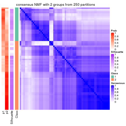
consensus_heatmap(res, k = 3)
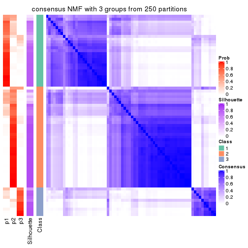
consensus_heatmap(res, k = 4)
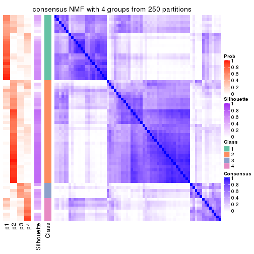
consensus_heatmap(res, k = 5)
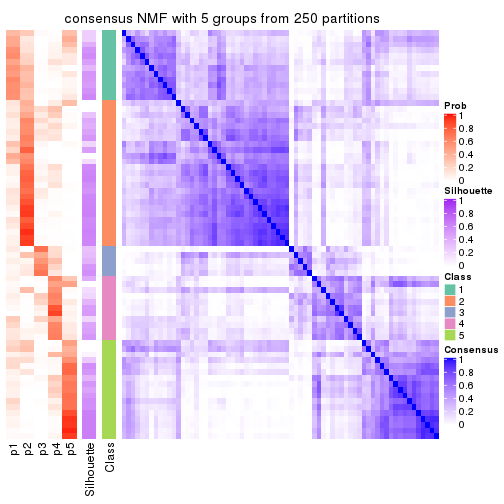
consensus_heatmap(res, k = 6)
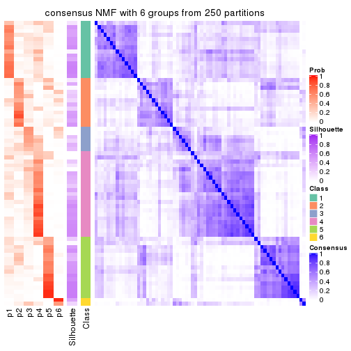
Heatmaps for the membership of samples in all partitions to see how consistent they are:
membership_heatmap(res, k = 2)
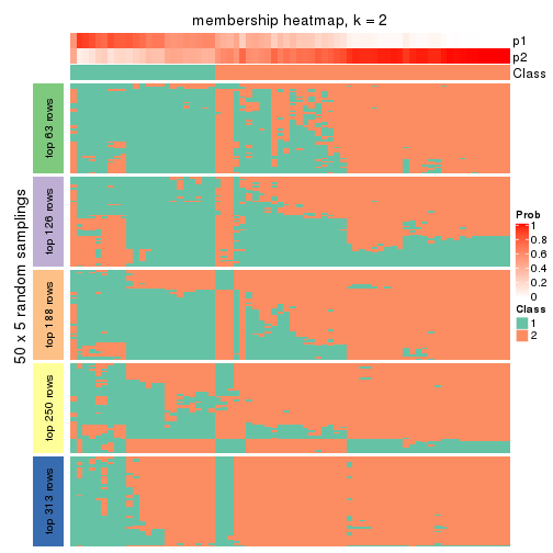
membership_heatmap(res, k = 3)
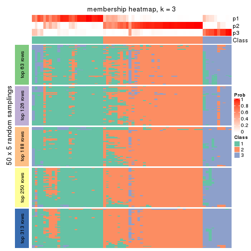
membership_heatmap(res, k = 4)
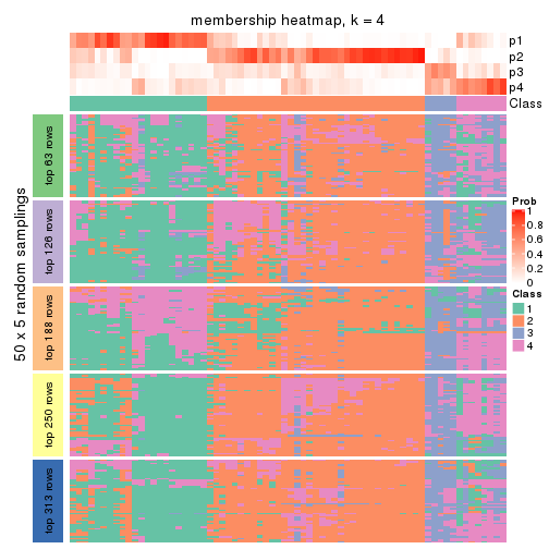
membership_heatmap(res, k = 5)
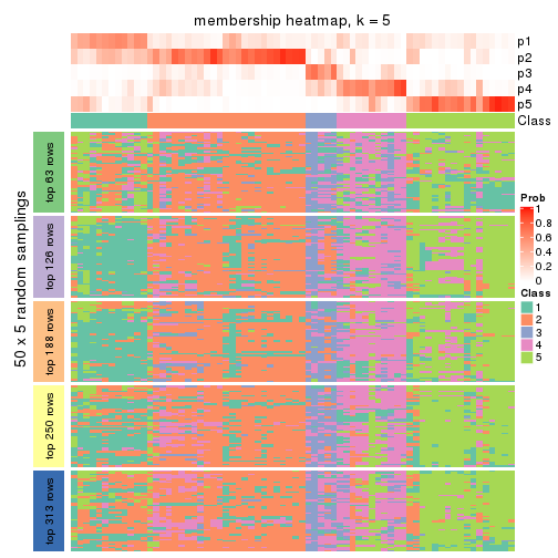
membership_heatmap(res, k = 6)
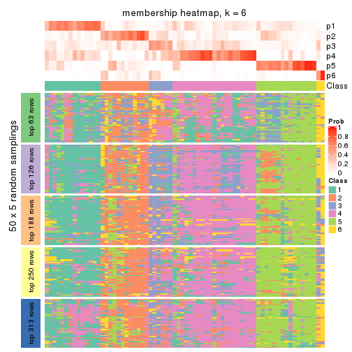
As soon as we have had the classes for columns, we can look for signatures which are significantly different between classes which can be candidate marks for certain classes. Following are the heatmaps for signatures.
Signature heatmaps where rows are scaled:
get_signatures(res, k = 2)
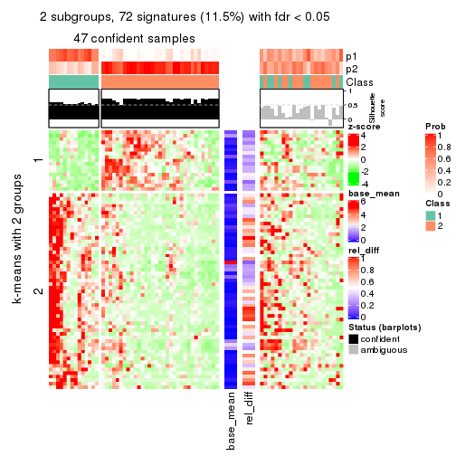
get_signatures(res, k = 3)
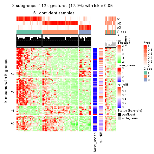
get_signatures(res, k = 4)
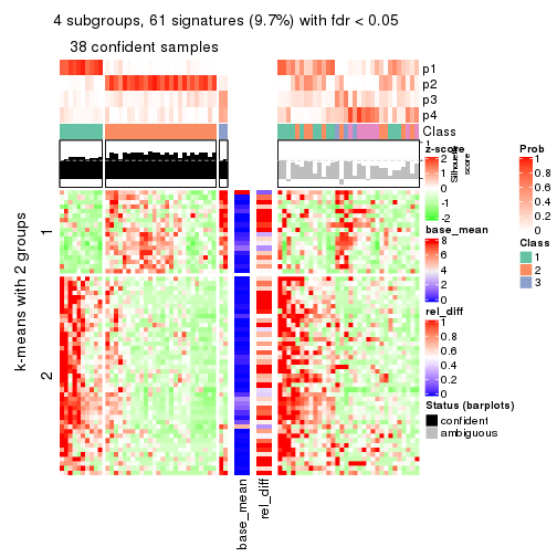
get_signatures(res, k = 5)
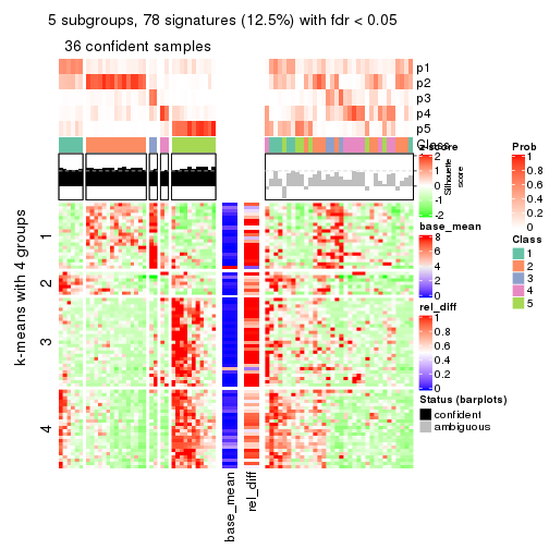
get_signatures(res, k = 6)
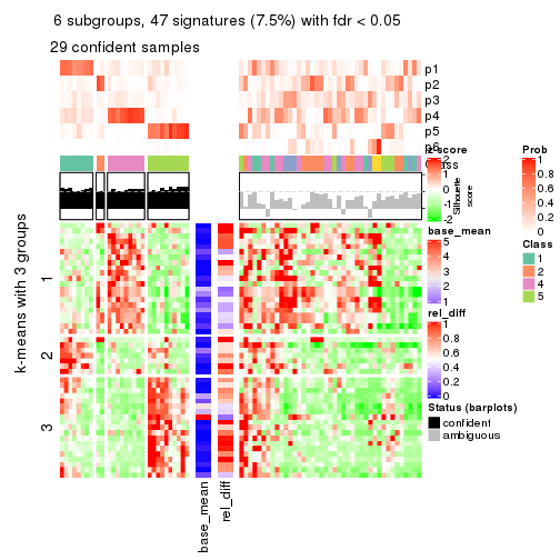
Signature heatmaps where rows are not scaled:
get_signatures(res, k = 2, scale_rows = FALSE)
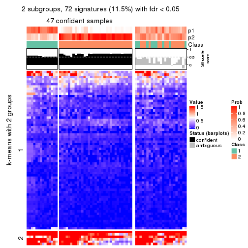
get_signatures(res, k = 3, scale_rows = FALSE)
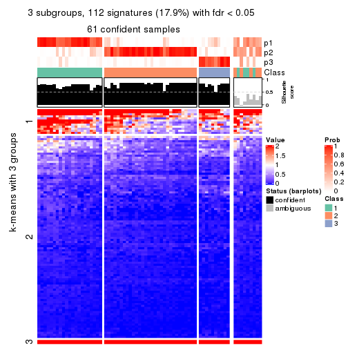
get_signatures(res, k = 4, scale_rows = FALSE)
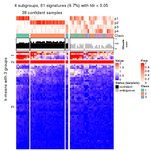
get_signatures(res, k = 5, scale_rows = FALSE)
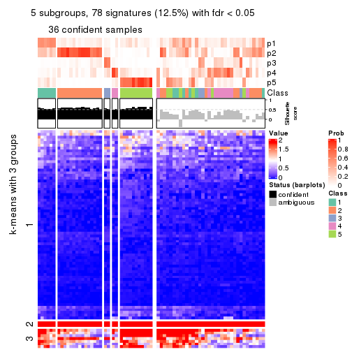
get_signatures(res, k = 6, scale_rows = FALSE)
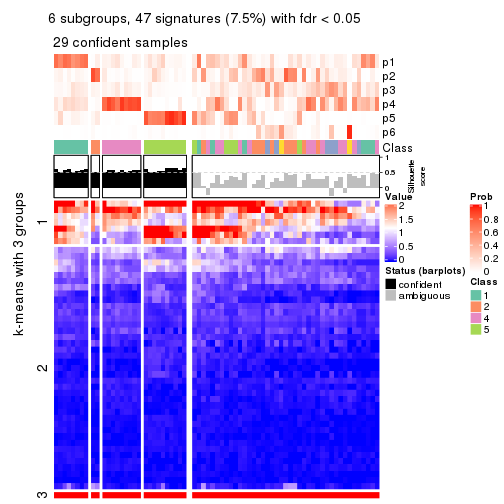
Compare the overlap of signatures from different k:
compare_signatures(res)
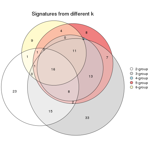
get_signature() returns a data frame invisibly. TO get the list of signatures, the function
call should be assigned to a variable explicitly. In following code, if plot argument is set
to FALSE, no heatmap is plotted while only the differential analysis is performed.
# code only for demonstration
tb = get_signature(res, k = ..., plot = FALSE)
An example of the output of tb is:
#> which_row fdr mean_1 mean_2 scaled_mean_1 scaled_mean_2 km
#> 1 38 0.042760348 8.373488 9.131774 -0.5533452 0.5164555 1
#> 2 40 0.018707592 7.106213 8.469186 -0.6173731 0.5762149 1
#> 3 55 0.019134737 10.221463 11.207825 -0.6159697 0.5749050 1
#> 4 59 0.006059896 5.921854 7.869574 -0.6899429 0.6439467 1
#> 5 60 0.018055526 8.928898 10.211722 -0.6204761 0.5791110 1
#> 6 98 0.009384629 15.714769 14.887706 0.6635654 -0.6193277 2
...
The columns in tb are:
which_row: row indices corresponding to the input matrix.fdr: FDR for the differential test. mean_x: The mean value in group x.scaled_mean_x: The mean value in group x after rows are scaled.km: Row groups if k-means clustering is applied to rows.UMAP plot which shows how samples are separated.
dimension_reduction(res, k = 2, method = "UMAP")
dimension_reduction(res, k = 3, method = "UMAP")
dimension_reduction(res, k = 4, method = "UMAP")
dimension_reduction(res, k = 5, method = "UMAP")
dimension_reduction(res, k = 6, method = "UMAP")
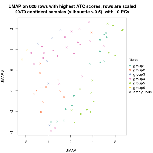
Following heatmap shows how subgroups are split when increasing k:
collect_classes(res)
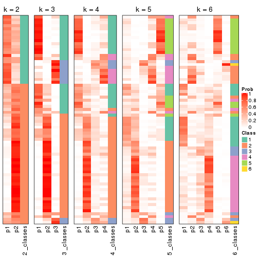
If matrix rows can be associated to genes, consider to use functional_enrichment(res,
...) to perform function enrichment for the signature genes. See this vignette for more detailed explanations.
sessionInfo()
#> R version 3.6.0 (2019-04-26)
#> Platform: x86_64-pc-linux-gnu (64-bit)
#> Running under: CentOS Linux 7 (Core)
#>
#> Matrix products: default
#> BLAS: /usr/lib64/libblas.so.3.4.2
#> LAPACK: /usr/lib64/liblapack.so.3.4.2
#>
#> locale:
#> [1] LC_CTYPE=en_GB.UTF-8 LC_NUMERIC=C LC_TIME=en_GB.UTF-8
#> [4] LC_COLLATE=en_GB.UTF-8 LC_MONETARY=en_GB.UTF-8 LC_MESSAGES=en_GB.UTF-8
#> [7] LC_PAPER=en_GB.UTF-8 LC_NAME=C LC_ADDRESS=C
#> [10] LC_TELEPHONE=C LC_MEASUREMENT=en_GB.UTF-8 LC_IDENTIFICATION=C
#>
#> attached base packages:
#> [1] grid stats graphics grDevices utils datasets methods base
#>
#> other attached packages:
#> [1] genefilter_1.66.0 ComplexHeatmap_2.3.1 markdown_1.1 knitr_1.26
#> [5] GetoptLong_0.1.7 cola_1.3.2
#>
#> loaded via a namespace (and not attached):
#> [1] circlize_0.4.8 shape_1.4.4 xfun_0.11 slam_0.1-46
#> [5] lattice_0.20-38 splines_3.6.0 colorspace_1.4-1 vctrs_0.2.0
#> [9] stats4_3.6.0 blob_1.2.0 XML_3.98-1.20 survival_2.44-1.1
#> [13] rlang_0.4.2 pillar_1.4.2 DBI_1.0.0 BiocGenerics_0.30.0
#> [17] bit64_0.9-7 RColorBrewer_1.1-2 matrixStats_0.55.0 stringr_1.4.0
#> [21] GlobalOptions_0.1.1 evaluate_0.14 memoise_1.1.0 Biobase_2.44.0
#> [25] IRanges_2.18.3 parallel_3.6.0 AnnotationDbi_1.46.1 highr_0.8
#> [29] Rcpp_1.0.3 xtable_1.8-4 backports_1.1.5 S4Vectors_0.22.1
#> [33] annotate_1.62.0 skmeans_0.2-11 bit_1.1-14 microbenchmark_1.4-7
#> [37] brew_1.0-6 impute_1.58.0 rjson_0.2.20 png_0.1-7
#> [41] digest_0.6.23 stringi_1.4.3 polyclip_1.10-0 clue_0.3-57
#> [45] tools_3.6.0 bitops_1.0-6 magrittr_1.5 eulerr_6.0.0
#> [49] RCurl_1.95-4.12 RSQLite_2.1.4 tibble_2.1.3 cluster_2.1.0
#> [53] crayon_1.3.4 pkgconfig_2.0.3 zeallot_0.1.0 Matrix_1.2-17
#> [57] xml2_1.2.2 httr_1.4.1 R6_2.4.1 mclust_5.4.5
#> [61] compiler_3.6.0